How Transformers Implement Induction Heads: Approximation and Optimization Analysis

Abstract

Transformers have demonstrated exceptional in-context learning capabilities, yet the theoretical understanding of the underlying mechanisms remain limited. A recent work (Elhage et al., 2021) identified a “rich” in-context mechanism known as induction head, contrasting with “lazy” $n$-gram models that overlook long-range dependencies. In this work, we provide both approximation and optimization analyses of how transformers implement induction heads. In the approximation analysis, we formalize both standard and generalized induction head mechanisms, and examine how transformers can efficiently implement them, with an emphasis on the distinct role of each transformer submodule. For the optimization analysis, we study the training dynamics on a synthetic mixed target, composed of a 4-gram and an in-context 2-gram component. This setting enables us to precisely characterize the entire training process and uncover an abrupt transition from lazy (4-gram) to rich (induction head) mechanisms as training progresses.

1 Introduction

Transformer, introduced by Vaswani et al. (2017), have achieved remarkable success across various domains, including natural language processing, computer vision, and scientific computing. An emergent observation is that transformers, trained on trillions of tokens, can perform (few-shot) in-context learning (ICL), which makes prediction based on the contextual information without needing model retraining (Brown et al., 2020). This ICL ability is widely regarded as crucial for enabling large language models (LLMs) to solve reasoning tasks, representing a key step toward more advanced artificial intelligence.

To understand how transformers implement ICL, Elhage et al. (2021) and Olsson et al. (2022) identified a simple yet powerful mechanism known as induction head. Specifically, given an input sequence [$\cdots$ab$\cdots$a], an induction head predicts b as the next token by leveraging the prior occurrence of the pattern ab in the context, effectively modeling an in-context bi-gram. In contrast, traditional $n$-gram model (Shannon, 1948) (with a small $n$) utilizes only a limited number of recent tokens to predict the next token, which is context-independent and inevitably overlooks long-range dependence. Based on the extent of context utilization, we categorize $n$-gram model as a “lazy” mechanism, whereas the induction head represents a more “rich” mechanism.

Practically, induction heads have been demonstrated to play a critical role in enabling LLMs’ ICL capabilities (Song et al., 2024; Crosbie and Shutova, 2024), and even used to test new LLM architectures (Gu and Dao, 2023). Theoretically, induction heads also serve as a controllable tool for understanding various aspects of LLMs, such as multi-step reasoning (Sanford et al., 2024b) and inductive biases of different architectures (Jelassi et al., 2024).

In this paper, we aim to provide a comprehensive analysis of how transformers can efficiently implement induction heads. The first key problem is to rigorously formalize induction heads and evaluate the efficiency of transformers in representing them. According to Elhage et al. (2021), the original induction head can be implemented using a two-layer, twelve-head transformer without feed-forward networks (FFNs). However, practical scenarios demand more powerful induction heads. Thus, it is crucial to generalize the mechanism behind and explore how different transformer submodules, such as varying the number of attention heads or incorporating FFNs, impact the transformer’s ability to implement them. This forms our first research objective:

(Approximation). Investigate how two-layer transformers express the induction head mechanism and its potential variants.

The next problem is to investigate the dynamics of transformers in learning induction heads. The pioneering works by Elhage et al. (2021) and Olsson et al. (2022) demonstrated that transformers undergo an abrupt phase transition to learning induction heads. A recent empirical study on synthetic datasets replicate this behavior, further showing that 2-gram is always learned prior to induction heads (Bietti et al., 2024). However, a rigorous theoretical analysis of this learning progression is still lacking. Closing this gap forms our second research objective:

(Optimization). Understand how transformers transition from relying on $n$-gram patterns to employing the induction head mechanism as training progresses.

Focusing on these two key problems, in this paper, we make the following contributions:

• Approximation analysis: how transformers express induction heads. We consider three types of induction heads with varying complexities. First, we show that two-layer, single-head transformers without FFNs can efficiently approximate the vanilla induction head (Elhage et al., 2021). We then introduce two generalized induction heads, which leverage richer in-context $n$-gram information and incorporate a general similarity function. Our analysis clarifies the distinct roles of multihead attention, positional encoding, dot-product structure, and FFNs in implementing these generalized induction heads.

• Optimization analysis: how learning undergoes a sharp transition from $n$-gram to induction head. We study the learning dynamics of a two-layer transformer without FFNs for a mixed target, composed of a 4-gram and an in-context 2-gram component. This toy setting allows us to capture the entire training process precisely. Specifically, we show that learning progresses through four phases: partial learning of the 4-gram, plateau of induction head learning, emergence of the induction head, and final convergence, showcasing a sharp transition from 4-gram to induction head. Our analysis identifies two key drivers of the transition: 1) time-scale separation due to low- and high-order parameter dependencies in self-attention, and 2) speed differences caused by the relative proportions of the two components in the mixed target. Additionally, in our analysis, we introduce a novel Lyapunov function that exploits the unique structure of self-attention, which may be of independent interest.

2 Related Works

Empirical observations of induction head. The induction head mechanism was first identified by Elhage et al. (2021) in studying how two-layer transformers perform language modeling. Subsequently, Olsson et al. (2022) conducted a more systematic investigation, revealing two key findings: 1) induction head emerges abruptly during training, and 2) induction head plays a critical role in the development of in-context learning capabilities. To obtain a fine-grained understanding of how induction head emerges during training, recent studies have developed several synthetic settings (Reddy, 2024; Edelman et al., 2024; Bietti et al., 2024). Particularly, Bietti et al. (2024) successfully reproduced the fast learning of (global) bigrams and the slower development of induction head. Despite these efforts, a comprehensive theoretical understanding of how the induction head operates in two-layer transformers and how it is learned during training remains elusive.

Expressiveness of transformers. Theoretically, Dehghani et al. (2019); Pérez et al. (2021); Wei et al. (2022) explored the Turing-completeness of transformers; Yun et al. (2019) established the universal approximation property of transformers. Subsequent studies examined the efficiency of transformers in representing specific functions or tasks, such as sparse functions (Edelman et al., 2022), targets with nonlinear temporal kernels (Jiang and Li, 2023), practical computer programs (Giannou et al., 2023), long but sparse memories (Wang and E, 2024), induction head (Sanford et al., 2024a; b; Rajaraman et al., 2024), and memorization and reasoning (Chen and Zou, 2024). Besides, many studies suggest that transformers achieve in-context learning by approximating gradient-based iterations across various layers (Garg et al., 2022; Akyürek et al., 2022; Von Oswald et al., 2023; Mahankali et al., 2023; Bai et al., 2023; Shen et al., 2023). Besides, several studies explored the limitation of transformer’s expressivity, particularly in modeling formal languages or simulating circuits (Hahn, 2020; Weiss et al., 2021; Bhattamishra et al., 2020; Merrill et al., 2022; Merrill and Sabharwal, 2023). Among all these works, the most closely related to ours are Rajaraman et al. (2024), which examined a generalized induction head similar to our Eq. (6). Specifically, they showed that multi-layer transformers with single-head attention can implement this mechanism. In contrast, we prove that two-layer transformers are sufficient if multihead attention is used.

Training dynamics of transformers. To gain insights into the dynamics of training transformers, several studies have analyzed simplified transformers on toy tasks. These tasks include learning distinct/common tokens (Tian et al., 2023), leaning balance/inblanced features (Huang et al., 2023), linear regression task (Zhang et al., 2023; Ahn et al., 2024), multi-task linear regression (Chen et al., 2024a), binary classification (Li et al., 2024), Transformer with diagonal weights (Abbe et al., 2024), learning causal structure (Nichani et al., 2024), sparse token selection task (Wang et al., 2024), and learning $n$-gram Markov chain (Chen et al., 2024b). Additionally, studies such as Ataee Tarzanagh et al. (2023); Tarzanagh et al. (2023); Vasudeva et al. (2024) have analyzed settings where transformers converge to margin maximization solutions and Thrampoulidis (2024) examined the implicit bias of next-token prediction. Among these works, the most closely related to ours are Nichani et al. (2024) and Chen et al. (2024b), which proved that two-layer transformers can converge to induction head solutions. In this work, we explore a setting where the target is a mixture of 4-gram and induction head. We show that two-layer transformers can effectively converge to this mixed target and provide a precise description of the learning process associated with each component. Importantly, we are able to capture the abrupt transition from learning 4-gram patterns to mastering the induction head mechanism—a critical phase in the learning of induction heads, as highlighted in previous studies (Elhage et al., 2021; Olsson et al., 2022).

3 Preliminaries

Notations. For $k\in\mathbb{N}^{+}$, let $[k]=\{1,2,\dots,k\}$. For a vector $v$, we denote by $\left\|v\right\|_{p}$ the $\ell_{p}$ norm, where $1\leq p\leq\infty$. For a matrix $A=(a_{i,j})$, we denote by $\|A\|$, $\|A\|_{F}$ the spectral and Frobenius norms, respectively; let $\|A\|_{1,1}=\sum_{i,j}|a_{i,j}|$. We use standard big-O notations $\mathcal{O},\Omega,\Theta$ to hide absolute positive constants, and use $\tilde{\mathcal{O}},\tilde{\Omega},\tilde{\Theta}$ to further hide logarithmic constants.

Sequence modeling. Given a sequence of tokens $(x_{1},x_{2},x_{3},\dots)$ with each token lying in $\mathbb{R}^{d}$, let $X_{L}=(x_{1},x_{2},\dots,x_{L})\in\mathbb{R}^{d\times L}$ and $X_{m:n}=(x_{m},x_{m+1},\dots,x_{n})\in\mathbb{R}^{d\times(n-m+1)}$. Then, we consider the next-token prediction task: predict $x_{L+1}$ using $X_{L}=(x_{1},x_{2},\dots,x_{L})$.

In a $n$-gram model (Shannon, 1948), the conditional probability of predicting the next token is given by $p(x_{L+1}|X_{L})=p(x_{L+1}|X_{L-n+2:L})$, meaning that the prediction depends only on the most recent $n-1$ tokens. In practice, the value of $n$ is typically small (e.g., 2, 3, or 4), as the computational cost of $n$-gram models grows exponentially with $n$. However, $n$-gram models with small $n$ cannot capture long-range interactions, leading to inferior performance in sequence modeling.

Transformer is designed to more efficiently capture long-range dependencies in sequence modeling (Vaswani et al., 2017). Specifically, given an $L$-token input sequence $X=(x_{1},\cdots,x_{L})\in\mathbb{R}^{d\times L}$, an $U$-layer transformer TF processes it as follows. First, each input token is embedded into a higher-dimensional space through an embedding layer:

$$x_{s}^{(0)}=W_{E}x_{s}+b_{E},\ s\in[L],\ \text{ with }W_{E}\in\mathbb{R}^{D\times d},b_{E}\in\mathbb{R}^{D}.$$

Next, the $U$-layer attention blocks process the embedded sequence $X^{(0)}=(x_{1}^{(0)},\cdots,x_{L}^{(0)})$ as follows, and the output of the final layer is taken as the output sequence ${\textnormal{{TF}}}(X)=X^{(L)}\in\mathbb{R}^{D\times L}$:

$$X^{(u-\frac{1}{2})} =X^{(u-1)}+{\textnormal{{SA}}}^{(u)}(X^{(u-1)}),\quad u\in[U];$$ (1)

$$X^{(u)} =X^{(u-\frac{1}{2})}+\textnormal{{FFN}}^{(u)}(X^{(u-\frac{1}{2})}),\quad u\in[U].$$

Here, $\textnormal{{FFN}}^{(u)}$ denotes a (point-wise) two-layer FFN of width $M$, and ${\textnormal{{SA}}}^{(u)}$ represents the multi-head self-attention operation. Specifically, when applied to a sequence $Z=(z_{1},\cdots,z_{L})\in\mathbb{R}^{D\times L}$, ${\textnormal{{SA}}}^{(l)}$ operates it as follows:

$${\textnormal{{SA}}}^{(u)}(Z)= W_{O}^{(u)}\sum_{h=1}^{H_{u}}{\textnormal{{SA}}}^{(u,h)}(Z),$$ (2)

$${\textnormal{{SA}}}^{(u,h)}(Z)= \left(W_{V}^{(u,h)}Z\right){\rm softmax}\left(\left\langle W_{Q}^{(u,h)}Z,W_{K}^{(u,h)}Z\right\rangle+R^{(u,h)}\right),$$

where $W_{Q}^{(u,h)},W_{K}^{(u,h)},W_{V}^{(u,h)},W_{O}^{(u)}\in\mathbb{R}^{D\times D}$ correspond to the query, key, value and output matrices of the $(u,h)$-th head, respectively. ${\rm softmax}$ represents taking softmax normalization across columns. $\left\langle W_{Q}^{(u,h)}X,W_{K}^{(u,h)}X\right\rangle$ is called the dot-product (DP) structure. Furthermore, $R^{(u,h)}=(R_{i,j}^{(u,h)})\in\mathbb{R}^{L\times L}$ denotes the additive relative positional encoding matrix, which satisfies $R_{i,j}^{(u,h)}=-\infty$ if $i\leq j$ for the next-token prediction task.

Relative positional encoding (RPE). In this work, we focus on the Alibi RPE (Press et al., 2022), where $R_{ij}^{(u,h)}$ follows a Toeplitz structure, i.e. $R_{ij}^{(u,h)}=\phi(i-j;p^{(u,h)})$ for $i,j\in[L]$. Here, $p^{(u,h)}$’s are learnable parameters and we consider $\phi(\cdot;p)$ of the following form:

$$\phi(z;p)=\begin{cases}-p\cdot(z-1)&\text{ if }z\geq 1\\ -\infty&\text{\ otherwise}\end{cases}.$$ (3)

Note that we adopt Alibi RPE only for simplicity and our results can be easily extended to other additive RPEs, such as T5 (Raffel et al., 2020).

4 Formulation and Approximation of Induction Head

In this section, we formalize three types of induction head mechanisms with varying levels of complexity. We then theoretically investigate how two-layer single- or multi-head transformers, with or without FFNs, can efficiently implement these mechanisms, highlighting the distinct roles of different transformer submodules

4.1 Vanilla Induction Heads

The original induction head, proposed in Elhage et al. (2021); Olsson et al. (2022), is regarded as one of the key mechanisms to implement ICL and reasoning. This induction head suggests that two-layer multi-head transformers without FFNs can execute a simple in-context algorithm to predict the next token b from a context [$\cdots$ab$\cdots$a] through retrieval, copying, and pasting, based on in-context bi-gram pairs, as illustrated in Figure 1.

Figure 1: An illustrative example of the induction head (taken from Elhage et al. (2021)). A pre-trained two-layer eight-head transformer without FFNs proceeds the context [$\cdots$. The D] by retrieving the preceding information most relevant to the current token (D), then copying and pasting the subsequent token (the green urs) as the current prediction.

Formulation of $\textnormal{{IH}}_{2}$. Based on the phenomenon illustrated in Figure 1, we define the vanilla induction head $\textnormal{{IH}}_{2}:\cup_{L\in\mathbb{N}^{+}}\mathbb{R}^{d\times L}\mapsto\mathbb{R}^{d}$ as follows:

$$\textnormal{{IH}}_{2}(X_{L})=\sum_{s=2}^{L-1}{\rm softmax}\big{(}x_{L}^{\top}W^{\star}x_{s-1}\big{)}x_{s}.$$ (4)

Specifically, $\textnormal{{IH}}_{2}$ retrieves in-context information based on the similarities of in-context bi-gram pairs $\{(x_{s},x_{L})\}_{s=1}^{L-2}$. Note that the magnitude of matrix $W^{\star}$ controls the sparsity of retrieval, since increasing $\|W^{\star}\|$ causes the softmax output to concentrate as a delta measure over the preceding tokens. Additionally, $\textnormal{{IH}}_{2}$ can handle input sequences of arbitrary length.

This model retrieves previous tokens $x_{s-1}$’s that are similar to the current token $x_{L}$ based on a dot-product similarity, and then copies and pastes $x_{s-1}$’s subsequent token $x_{s}$ as the current prediction $x_{L+1}$. The softmax normalization is applied to the similarity scores to ensure the sparsity of relevant information. For example, in Figure 1, the current token $x_{L}$ is D, and the model retrieves previous tokens similar to D, copying and pasting its subsequent token urs as the prediction.

Comparison with previous formulations. As shown in Figure 1, the current token D appears multiple times in the preceding context, and the induction head detects all occurrences of D. Our formulation (4) captures this behavior, as the softmax scores for all preceding D are identical. In contrast, previous formulations, such as Sanford et al. (2024a) and Sanford et al. (2024b), focus solely on the most recent occurrence of D, neglecting this multi-occurrence aspect.

Measure of approximation. Consider a target function $\textsf{H}:\cup_{L\in\mathbb{N}^{+}}\mathbb{R}^{d\times L}\mapsto\mathbb{R}^{d}$, where $d$ is the token dimension and $L$ denotes the sequence length. Given an input sequence $X\in\mathbb{R}^{d\times L}$, transformer TF approximates $\textsf{H}(X)$ using its last output token, i.e., ${\textnormal{{TF}}}_{-1}(X)\in\mathbb{R}^{d}$. To quantify the approximation error, we define the following metric: for $1\leq p\leq+\infty$,

$$\left|\!\left|\!\left|\textsf{H}-{\textnormal{{TF}}}\right|\!\right|\!\right|_{L,p}:=\big{(}\mathbb{E}_{X_{L}}[\|\textsf{H}(X_{L})-{\textnormal{{TF}}}_{-1}(X_{L})\|_{\infty}^{p}]\big{)}^{1/p}.$$ (5)

The next theorem shows that a two-layer single-head transformer without FFNs suffices to implement vanilla induction heads.

Theorem 4.1 (two-layer single-head TF w/o FFNs).

Let $\textnormal{{IH}}_{2}$ satisfy Eq. (4). Then exists a constant $C>0$ and a two-layer single-head transformer TF (without FFNs), with $D=2d$, $W_{K}^{(1,1)}=W_{Q}^{(1,1)}=0$, $p^{(2,1)}=0$, and $\|W_{K}^{(2,1)}\|,\|W_{Q}^{(2,1)}\|\leq\mathcal{O}(1,\|W^{\star}\|_{F})$, such that

$$\sup_{L\in\mathbb{N}^{+}}\left|\!\left|\!\left|\textnormal{{IH}}_{2}-{\textnormal{{TF}}}\right|\!\right|\!\right|_{L,\infty}\leq\frac{C}{e^{p^{(1,1)}}}.$$

It is worth noting that the approximation efficiency is independent of the sequence length. The proof is provided in Appendix A.1, offering the following insights into how two-layer single-head transformers without FFNs implement vanilla induction heads:

• In the first layer, RPE in SA is used to approximate the memory kernel: $\rho(\cdot)=\mathbb{I}\{\cdot=1\}$. Thus, SA can capture the preceding token via $x_{s-1}=\sum_{j\geq 1}x_{s-j}\rho(j)$ for each token $x_{s}$, which is crucial for future comparison. Notably, DP in this layer is not essential and can be omitted.

• In the second layer, DP is used to calculate the similarity $\left\langle\cdot,W^{\star}\cdot\right\rangle$. Then SA can compare the current token $x_{L}$ with all previous tokens to identify those tokens that are similar to $x_{L}$. If a token is found to be similar to $x_{L}$, the model copies its subsequent token and pastes it as the current prediction. Notably, RPE in this layer is not essential and can be omitted.

Remark 4.2 (Alignment with experimental findings).

Our theoretical analysis is consistent with the experimental observations reported in Elhage et al. (2021). Specifically, the experiments there demonstrate that SA in the first layer attends to adjacent tokens, while SA in the second layer retrieves information related to the current token. Our analysis identifies components responsible for these two operations, and reveals that single-head transformers suffice to perform them efficiently.

4.2 Generalized Induction Heads: In-context $n$-gram and Generic Similarity

Although the standard induction head defined in Eq. (4) is intuitive, it exhibits notable limitations: 1) it retrieves only a single token, potentially missing complete local information and leading to false retrievals; 2) it relies solely on the dot-product to measure the similarity between two tokens, which is not sufficiently general.

Formulation of $\textnormal{{IH}}_{n}$. Motivated by the limitation 1) above, we define a generalized induction head:

$$\textnormal{{IH}}_{n}(X_{L})=\sum_{s=n}^{L-1}{\rm softmax}\Big{(}X_{L-n+2:L}^{\top}W^{\star}X_{s-n+1:s-1}\Big{)}x_{s},$$ (6)

where the patch $X_{s-n+1:s-1}$ incorporates richer local information near $x_{s}$ and $X_{L-n+2:L}$ denotes the current patches. This formulation is more general than Eq. (4), which only focuses on $x_{s-1}$. This induction head operates based on the similarity between the $n$-gram pairs: $(X_{s-n+1:s-1};X_{L-n+2:L})$ for $s=n,\dots,L-1$.

Integrating richer local information facilitates more accurate information retrieval. The model (6) retrieves previous $(n-1)$-token patch that are similar to the current $(n-1)$-token patch, thereby generalizing the vanilla induction head (4), which considers only single-token retrieval. For example, as depicted in Figure 1, if the current local information is The D (comprising two tokens), and prior local information such as Mr D and Mrs D is identified as similar to The D, transformer would copy and paste their subsequent token, urs, as the prediction.

Theorem 4.3 (two-layer multi-head TF w/o FFNs).

Let $\textnormal{{IH}}_{n}$ satisfy Eq. (6). Then for any $q\in\mathbb{N}^{+}$ , there exists a constant $C_{q,n}>0$ and a two-layer $H$-head transformer ${\textnormal{{TF}}}(\cdot)$ (without FFNs), with $D=nd$, such that:

$$\sup_{L\in\mathbb{N}^{+}}\left|\!\left|\!\left|\textnormal{{IH}}_{n}-{\textnormal{{TF}}}\right|\!\right|\!\right|_{L,\infty}\leq\frac{C_{q,n}}{H^{q}}.$$

This theorem demonstrates that two-layer multi-head transformers, even without FFNs, can efficiently implement the generalized induction head (6). Notably, the approximation error scales as $\mathcal{O}(H^{-q})$, where $q$ can be arbitrarily large. The proof of this theorem is provided in Appendix A.2.

The role of multiple heads. In Theorem 4.3, multiple heads are employed in the first layer to approximate the $n$-gram interaction, represented by the $n-1$ memory kernels $\{\rho_{j}:=\mathbb{I}\{\cdot=j\}\}_{j=1}^{n-1}$. Thus, TF can capture $n-1$ preceding tokens via $x_{s-j}=\sum_{k\geq 1}x_{s-k}\rho_{j}(k)$ for $j\in[n-1]$. Intuitively, as $n$ increases, more memory kernels are required for accurate approximation, necessitating more attention heads. In contrast, Theorem 4.1 only requires approximating a single memory kernel $\mathbb{I}\{\cdot=1\}$, which can be efficiently achieved using a single attention head.

Recently, Rajaraman et al. (2024) explored a generalized induction head similar to Eq. (6) and showed that multi-layer single-head transformers can implement it. In contrast, our Theorem 4.3 demonstrates that two layers suffice if multi-head self-attention is adopted.

Formulation of $\textnormal{{GIH}}_{n}$. Building on the formulation (6), and motivated by the limitation 2) above, we further consider the following generalized induction head:

$$\textnormal{{GIH}}_{n}(X_{L})=\sum_{s=n}^{L-1}{\rm softmax}\Big{(}g\big{(}X_{L-n+2:L},X_{s-n+1:s-1}\big{)}\Big{)}x_{s},$$ (7)

where $g:\mathbb{R}^{D\times(n-1)}\times\mathbb{R}^{D\times(n-1)}\to\mathbb{R}$ denotes a generic function measuring the similarity between two $(n-1)$-length patches.

This model retrieves previous relevant multi-token patch $X_{s-n+1:s-1}$ that is similar to the current multi-token patch $X_{L-n+2:L}$ , utilizing the generalized similarity function $g(\cdot,\cdot)$. This mechanism is more general than Eq. (6), which is limited to dot-product similarities. For instance, the use of general similarity $g$ enables the model to recognize not only synonymous but also antonymic semantics, thereby improving both the accuracy and diversity of in-context retrievals.

Theorem 4.4 (two-layer multi-head TF with FFNs).

Let $\textnormal{{GIH}}_{n}$ satisfy Eq. (7). Suppose the similarity function $g$ is $\alpha$-well-behaved (see Definition A.7). Then, for any $q\in\mathbb{N}^{+}$, there exist constants $A_{g,q,n},B_{g,\alpha}>0$ and a two-layer $H$-head transformer ${\textnormal{{TF}}}(\cdot)$ with FFNs of width $M$, such that

$$\left|\!\left|\!\left|\textnormal{{GIH}}_{n}-{\textnormal{{TF}}}\right|\!\right|\!\right|_{L,2}\leq\frac{A_{g,q,n}}{H^{q}}+\frac{B_{g,\alpha}L^{1/(1+2\alpha)}}{M^{\alpha/(1+3\alpha)}}.$$

This theorem establishes that if the similarity function $g$ is well-behaved, two-layer multi-head transformers with FFNs can efficiently implement the generalized induction head (7).

The role of FFNs. In contrast to Theorem 4.3, transformer models in Theorem 4.4 include FFNs. These FFN layers are used to approximate the similarity function $g$. Specifically, we consider the proper orthogonal decomposition (POD) of $g$, which can be viewed as an extension of the matrix singular value decomposition (SVD) applied to functions of two variables. For $g:\mathcal{I}\times\mathcal{I}\to\mathbb{R}$, its POD is $g(u,v)=\sum_{k=1}^{\infty}\sigma_{k}\phi_{k}(u)\psi_{k}(v)$, where $\phi_{k},\psi_{k}$ are orthonormal bases for $L^{2}(\mathcal{I})$ (see Appendix D for details). Intuitively, the FFN in the first layer is used to efficiently approximate $K$ bases ($\phi_{i}$’s and $\psi_{i}$’s). Then, in the second layer, DP in SA can approximately reconstruct $g$ by using the truncated sum $g(u,v)\approx\sum_{k=1}^{K}\sigma_{k}\phi_{k}(u)\psi_{k}(v)$. The complete proof is deferred to Appendix A.3.

5 The Transition from Lazy to Rich Mechanisms in Learning Induction Heads

In this section, we investigate the dynamics of learning induction heads using a transformer, particularly focusing on how this differs from $n$-gram learning. To facilitate the analysis, we consider a mixed target function that comprises a $4$-gram component and a vanilla induction head component as defined in Eq. (4). Specifically, we study the gradient flow dynamics of a two-layer multi-head transformer without FFNs on this task.

5.1 Setups

5.1.1 Mixed Target Function

Mixed target function. Let the input sequence be $X=(x_{1},\cdots,x_{L})\in\mathbb{R}^{1\times L}$. Our mixed target function $f^{\star}$ contains both a $4$-gram component $f_{\textnormal{{G}}_{4}}^{\star}$ and an in-context $2$-gram component $f_{\textnormal{{IH}}_{2}}^{\star}$:

$$f^{\star}(X):=\left(\frac{\alpha^{\star}}{1+\alpha^{\star}}f_{\textnormal{{G}}_{4}}^{\star}(X),\frac{1}{1+\alpha^{\star}}f_{\textnormal{{IH}}_{2}}^{\star}(X)\right)^{\top}\in\mathbb{R}^{2},$$ (8)

where $\alpha^{\star}>0$ represents the relative weight between the two components: $f_{\textnormal{{G}}_{4}}^{\star}(X)$ and $f_{\textnormal{{IH}}_{2}}^{\star}(X)$. Here, $f_{\textnormal{{G}}_{4}}^{\star}$ represents a $4$-gram component and $f_{\textnormal{{IH}}_{2}}^{\star}$ is given by the vanilla induction head (4) to represent a type of in-context 2-gram information:

$$f_{\textnormal{{G}}_{4}}^{\star}(X):=x_{T-2},\quad f_{\textnormal{{IH}}_{2}}^{\star}(X):=\sum_{s=2}^{L-1}{\rm softmax}\left(x_{L}{w^{\star}}^{2}x_{s-1}\right)x_{s}.$$

Note that $f_{\textnormal{{G}}_{4}}^{\star}$ denotes a “simplest” 4-gram target, where the next token is predicted according to the conditional probability $p(z|X)=p(z|x_{L},x_{L-1},x_{L-2})=\mathbb{I}\{z=x_{L-2}\}$.

Remark 5.1 (The reason for considering $4$-gram).

Note that our target includes a 4-gram component rather than simpler 2- or 3-gram components. As suggested by the experimental results in Elhage et al. (2021), for a learned two-layer transformer that implements vanilla induction head $\textnormal{{IH}}_{2}$, the first layer has extracted both $x_{L}$ and $x_{L-1}$, which can be outputted using the residual block. Thus, the 2- and 3-gram targets: $p(z|X)=\mathbb{I}\{z=x_{L}\}$ and $p(z|X)=\mathbb{I}\{z=x_{L-1}\}$ must be learned prior to the induction head. Hence we focus on the more challenging 4-gram target to avoid trivializing the learning process, though our analysis extends straightforwardly to the 2- or 3-gram scenarios.

Remark 5.2 (Extension).

Since the transformer studied in this section does not have FFNs, its expressive power is limited. Consequently, we only consider the simple but representative mixed target (8). However, (8) can be generalized to $f^{\star}(X)=F(f_{\textnormal{{G}}_{4}}^{\star}(X);f_{\textnormal{{IH}}_{2}}^{\star}(X))$, where $F$ is general nonlinear function. Such a form can be efficiently approximated by transformers with FFNs. We leave the optimization analysis under this general setting for future work.

5.1.2 Two-layer Multi-head Transformer with Reparameterization

Two-layer multi-head transformer w/o FFNs. We consider a simple two-layer multi-head transformer TF, where the first layer contains a single head ${\textnormal{{SA}}}^{(1,1)}$, and the second layer contain two heads ${\textnormal{{SA}}}^{(2,1)},{\textnormal{{SA}}}^{(2,2)}$. Given an input sequence $X=(x_{1},\cdots,x_{L})\in\mathbb{R}^{1\times L}$, it is first embedded as $X^{(0)}:=(X^{\top},0^{\top})\in\mathbb{R}^{2\times L}$. The model then processes the sequence as follows:

$$X^{(1)}= \ X^{(0)}+{\textnormal{{SA}}}^{(1,1)}(X^{(0)}),$$

$${\textnormal{{TF}}}(X)= \ {\textnormal{{SA}}}^{(2,1)}(X^{(1)})+{\textnormal{{SA}}}^{(2,2)}(X^{(1)}).$$

Reparameterization. Despite the simplification, the transformer above is still too complicated for dynamics analysis. To overcome this challenge, we adopt the reparametrization trick used in previous works (Tian et al., 2023; Huang et al., 2023; Chen et al., 2024b). Specifically, by Theorem 4.1 and its proof, the first layer does not require DP, and the second layer does not require RPE. Moreover, to express the $4$-gram component $f_{\textnormal{{G}}_{4}}^{\star}$, we only need an additional head without DP in the second layer. Therefore, we can reparameterize the model as follows:

• The first layer. This layer has only one trainable parameter $p^{(1,1)}$. In the unique head ${\textnormal{{SA}}}^{(1,1)}$, DP is removed by setting $W_{Q}^{(1,1)}=W_{K}^{(1,1)}=0$, and we let $W_{V}^{(1,1)}=\begin{pmatrix}0&0\\ 1&0\end{pmatrix}$. The output sequence of this layer given by $X^{(1)}=X^{(0)}+{\textnormal{{SA}}}^{(1,1)}(X^{(0)})=\begin{pmatrix}x_{1},\cdots,x_{L}\\ y_{1},\cdots,y_{L}\end{pmatrix}$, where

  $$y_{s}=\sum_{\tau=1}^{s-1}{\rm softmax}\left(-p^{(1,1)}(s-1-\tau)\right)x_{\tau},\ s\in[L],$$ (9)

  where $p^{(1,1)}$, used in RPE (3), is the unique trainable parameter in this layer.

• The second layer. This layer has 5 trainable parameters: $w_{V}^{(2,1)},w_{V}^{(2,2)},p^{(2,1)},w_{K}^{(2,2)},w_{Q}^{(2,2)}$ for parametrizing the two heads. The first head ${\textnormal{{SA}}}^{(2,1)}$ without DP is responsible to fit $f_{\textnormal{{G}}_{4}}^{\star}$, while the second head ${\textnormal{{SA}}}^{(2,2)}$ without RPE is responsible to fit $f_{\textnormal{{IH}}_{2}}^{\star}$. Specifically,

  $$W_{Q}^{(2,1)}=W_{K}^{(2,1)}=0,W_{V}^{(2,1)}=\begin{pmatrix}0&w_{V}^{(2,1)}\\ 0&0\end{pmatrix},p^{(2,2)}=0,W_{V}^{(2,2)}=\begin{pmatrix}w_{V}^{(2,2)}&0\\ 0&0\end{pmatrix}.$$

  Then the second layer processes $X^{(1)}$ and outputs the last token:

  $${\textnormal{{TF}}}_{-1}(X;\theta)=\begin{pmatrix}w_{V}^{(2,1)}\sum_{s=2}^{L-2}{\rm softmax}(-p^{(2,1)}(L-1-s))y_{s}\\ w_{V}^{(2,2)}\sum_{s=2}^{L-2}{\rm softmax}\left(x_{L}w_{Q}^{(2,2)}w_{K}^{(2,2)}x_{s-1}\right)x_{s}\end{pmatrix},$$ (10)

  where $y_{s}$ is given by (9). $p^{(2,1)},w_{V}^{(2,1)}$ are trainable parameters in ${\textnormal{{SA}}}^{(2,1)}$, while $w_{Q}^{(2,2)},w_{K}^{(2,2)},w_{V}^{(2,2)}$ are trainable parameters in ${\textnormal{{SA}}}^{(2,2)}$.

The set of all six trainable parameters across both layers is denoted by $\theta$.

5.1.3 Gradient Flow on Square Loss

We consider the Gaussian input and square loss, both of which are commonly used in analyzing transformer dynamics and ICL (Akyürek et al., 2022; Huang et al., 2023; Wang et al., 2024). The loss is defined as:

$$\mathcal{L}(\theta)=\frac{1}{2}\mathbb{E}_{X\sim\mathcal{N}(0,I_{L\times L})}\left[\left\|{\textnormal{{TF}}}_{-1}({X};\theta)-f^{\star}(X)\right\|_{2}^{2}\right],$$ (11)

To characterize the learning of $\textnormal{{G}}_{4}$ and $\textnormal{{IH}}_{2}$, we introduce the following two partial losses:

$$\mathcal{L}_{\textnormal{{G}}_{4}}(\theta)=\frac{1}{2}{\mathbb{E}}_{X}\left({\textnormal{{TF}}}_{-1,1}({X};\theta)-f_{1}^{\star}(X)\right)^{2},\ \mathcal{L}_{\textnormal{{IH}}_{2}}(\theta)=\frac{1}{2}{\mathbb{E}}_{X}\left({\textnormal{{TF}}}_{-1,2}({X};\theta)-f_{2}^{\star}(X)\right)^{2},$$

which correspond to the two dimensions in ${\textnormal{{TF}}}_{-1}({X};\theta)-f^{\star}(X)\in\mathbb{R}^{2}$, respectively. It follows that $\mathcal{L}(\theta)=\mathcal{L}_{\textnormal{{G}}_{4}}(\theta)+\mathcal{L}_{\textnormal{{IH}}_{2}}(\theta)$.

Gradient flow (GF). We analyze the GF for minimizing the objective (11):

$$\frac{{\textnormal{d}}\theta(t)}{{\textnormal{d}}t}=-\nabla\mathcal{L}(\theta(t)),\text{\ starting with\ }\theta(0)=(\sigma_{\rm init},\cdots,\sigma_{\rm init})^{\top},$$ (12)

where $0<\sigma_{\rm init}\ll 1$ is sufficiently small. Note that $\sigma_{\rm init}\neq 0$ prevents $\nabla\mathcal{L}(\theta(0))=0$.

Layerwise training paradigm. We consider a layerwise training paradigm in which, during each stage, only one layer is trained by GF. Specifically,

• Training Stage I: In this phase, only the parameter in the first layer, i.e., $p^{(1,1)}$, is trained.

• Training Stage II: In this phase,the first layer parameter $p^{(1,1)}$ keeps fixed and only parameters in the second layer are trained: $w_{V}^{(2,1)},w_{V}^{(2,2)},p^{(2,1)},w_{Q}^{(2,2)},w_{K}^{(2,2)}$.

This type of layerwise training has been widely used to study the training dynamics of neural networks, including FFN networks (Safran and Lee, 2022; Bietti et al., 2023; Wang et al., 2023) and transformers (Tian et al., 2023; Nichani et al., 2024; Chen et al., 2024b).

Lemma 5.3 (Training Stage I).

For the Training Stage I, $\lim\limits_{t\to+\infty}p^{(1,1)}(t)=+\infty$.

According to (9), this lemma implies that, at the end of Training Stage I, the first layer captures the preceding token $x_{s-1}$ for each token $x_{s}$, i.e., $y_{s}=x_{s-1}$. This property is crucial for transformers to implement induction heads and aligns with our approximation result in Theorem 4.1. The proof of Lemma 5.3 is deferred to Appendix B.

5.2 Training Stage II: Transition from $4$-gram to Induction Head

In this section, we analyze the dynamics in Training Stage II. We start from the following lemma:

Lemma 5.4 (Parameter balance).

In Training Stage II, it holds that ${w_{Q}^{(2,2)}}^{2}(t)\equiv{w_{K}^{(2,2)}}^{2}(t)$.

Lemma 5.4 is similar to the balance result for homogeneous networks (Du et al., 2018), and its proof can be found at the start of Appendix C. By this lemma, we can define $w_{KQ}^{(2,2)}:=w_{Q}\equiv w_{K}$. Additionally, Lemma 5.3 ensures that $p^{(1,1)}=+\infty$ holds during Stage II. For simplicity, we denote $w_{V_{1}}:=w_{V}^{(2,1)},w_{V_{2}}:=w_{V}^{(2,2)},p:=p^{(2,1)},w_{KQ}:=w_{KQ}^{(2,2)}$. Consequently, the training dynamics are reduced for four parameters

$${\theta}=\left(w_{V_{1}},w_{V_{2}},p,w_{KQ}\right),$$

where we still denote the set of parameters as $\theta$ without loss of ambiguity. Note that the problem remains highly non-convex due to the joint optimization of both inner parameters ($p,w_{KQ}$) and outer parameters ($w_{V_{1}},w_{V_{2}}$) in the two heads. In this stage, GF has a unique fixed point: $w_{V_{1}}=\frac{\alpha^{\star}}{1+\alpha^{\star}},w_{V_{2}}=\frac{1}{1+\alpha^{\star}},{p}=+\infty,w_{KQ}=w^{\star}$, which corresponds to a global minimizer of the objective (11).

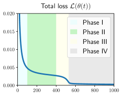
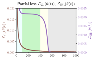
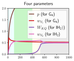
Figure 2: Visualization of the total loss, partial loss, and the parameter dynamics in our setting with $\alpha^{\star}=1,w^{\star}=0.49,\sigma_{\rm init}=0.01,L=1000$. The figure clearly shows that transformer learns the $4$-gram component first and then, starts to learn the induction head mechanism. Notably, the entire dynamics exhibit four phases.

As shown in Figure 2, a learning transition from the 4-gram mechanism to the induction head mechanism does occur in our setting. Moreover, the learning process exhibits a four-phase dynamics. The next theorem provides a precise characterization of the four phases, whose proof can be found in Appendix C.

Theorem 5.5 (Learning transition and $4$-phase dynamics).

Let $\alpha^{\star}=\Omega(1)$ and $w^{\star}=\mathcal{O}(1)$, and we consider the regime of small initialization ($0<\sigma_{\rm init}\ll 1$) and long input sequences ($L\gg 1$). Then we have the following results:

• Phase I (partial learning). In this phase, most of the $4$-gram component in the mixed target is learned, while a considerable number of induction head component have not yet been learned. Specifically, let $T_{\rm I}=\mathcal{O}(1)$, then we have the following estimates:

  $$\mathcal{L}_{\textnormal{{G}}_{4}}(\theta(T_{\rm I}))\leq 0.01\cdot\mathcal{L}_{\textnormal{{G}}_{4}}(\theta(0)),\quad\mathcal{L}_{\textnormal{{IH}}_{2}}(\theta(T_{\rm I}))\geq 0.99\cdot\mathcal{L}_{\textnormal{{IH}}_{2}}(\theta(0)).$$

• Phase II (plateau) + Phase III (emergence). In these two phases, the learning of the induction head first gets stuck in a plateau for $T_{\rm II}$ time, then is learned suddenly. Specifically, denoted by an observation time $T_{o}=\Theta(L)$, we have the following tight estimate of the duration:

  $$T_{\rm II} :=\inf\Big{\{}t>T_{o}:\mathcal{L}_{\textnormal{{IH}}_{2}}(\theta(t))\leq 0.99\cdot\mathcal{L}_{\textnormal{{IH}}_{2}}(\theta(T_{o}))\Big{\}}=\Theta\left((\alpha^{\star}+1)^{2}L\log(1/\sigma_{\rm init})/{w^{\star}}^{2}\right);$$

  $$T_{\rm III} :=\inf\Big{\{}t>T_{o}:\mathcal{L}_{\textnormal{{IH}}_{2}}(\theta(t))\leq 0.01\cdot\mathcal{L}_{\textnormal{{IH}}_{2}}(\theta(T_{o}))\Big{\}}=\Theta\left((\alpha^{\star}+1)^{2}L\log(1/\sigma_{\rm init})/{w^{\star}}^{2}\right).$$

  During these phases, the parameter $w_{KQ}$ (for learning $w^{\star}$ in $\textnormal{{IH}}_{2}$) increases exponentially:

  $$w_{KQ}(t)=\sigma_{{\rm init}}\cdot\exp\left(\Theta\left(\frac{{w^{\star}}^{2}t}{(1+\alpha^{\star})^{2}L}\right)\right),\ t<T_{\rm III}.$$

• Phase IV (convergence). In this phase, the loss convergences. Specifically, the following convergence rates hold for all $t>T_{\rm III}:$

  $${\mathcal{L}_{\textnormal{{G}}_{4}}(\theta(t))}=\mathcal{O}\left(\frac{1}{t}\right),\quad\mathcal{L}_{\textnormal{{IH}}_{2}}(\theta(t))=\mathcal{O}\left(\exp\left(-\Omega\left(\frac{{w^{\star}}^{2}t}{(1+\alpha^{\star})^{2}L}\right)\right)\right),$$

  and $\mathcal{L}(\theta(t))=\mathcal{L}_{\textnormal{{G}}_{4}}(\theta(t))+\mathcal{L}_{\textnormal{{IH}}_{2}}(\theta(t))$.

By this theorem, the $4$-gram mechanism is first learned, taking time $T_{\rm I}$. Then, the learning of the induction head mechanism enters a plateau, taking time $T_{\rm II}$, followed by a sudden emergence of learning, taking time $T_{\rm III}-T_{\rm II}$. Finally, the loss for both components converges to zero.

The clear learning transition. When any one of $L,\alpha^{\star},1/\sigma_{\rm init},1/w^{\star}$ is sufficiently large, Phase II lasts for $T_{\rm II}\gg 1$. During this phase, the $4$-gram component has been learned well but the induction head component remains underdeveloped, demonstrating a distinct learning transition. Moreover, Theorem 5.5 and its proof reveal two key factors that drive this transition:

• Time-scale separation due to high- and low-order parameter dependence in self attention. The learning of DP and RPE components differ in their parameter dependencies. DP component exhibits a quadratic dependence on the parameter $w_{KQ}$, while RPE component shows linear dependence on the parameter $p$. With small initialization $\sigma_{\rm init}\ll 1$, a clear time-scale separation emerges: $|\dot{w}_{KQ}|\sim w_{KQ}\ll 1$ (DP, slow dynamics) and $|\dot{p}|\sim 1$ (RPE, fast dynamics). Consequently, the induction head (fitted by DP) is learned much slower than the 4-gram component (fitted by RPE). This time-scale separation accounts for the term $\log(1/\epsilon_{\rm init})$ in the plateau time $T_{\rm II}$.

• Speed difference due to component proportions in the mixed target. The 4-gram target component and the induction-head component have differing proportions in the mixed target. A simple calculation shows: $\mathcal{L}_{\textnormal{{G}}_{4}}(0)\sim{\alpha^{\star}}^{2}/({1+\alpha^{\star}})^{2}$; If $w^{\star}=\mathcal{O}(1)$, then $\mathcal{L}_{\textnormal{{IH}}_{2}}(0)\sim{1}/[{(1+\alpha^{\star})^{2}L}]$. Notably, $\mathcal{L}_{\textnormal{{IH}}_{2}}(0)$ is significantly smaller than $\mathcal{L}_{\textnormal{{G}}_{4}}(0)$. This proportion disparity accounts for the $(1+\alpha^{\star})^{2}L$ term in the plateau time $T_{\rm II}$.

Proof idea. Our analysis relies on a precise description of the parameter trajectories, driven by two key observations: 1) the dynamics of two heads can be decoupled; 2) there exist a distinct transition point in the dynamics of each head, as shown in Figure 2 (right). These insights lead us to divide the analysis of each head into two phases: a monotonic phase and a convergence phase. Particularly, for the convergence phase, we introduce a novel Lyapunov function that leverages the unique dynamical structure of self-attention. This Lyapunov function may be of independent interest and offers potential for studying broader issues in self-attention dynamics.

6 Conclusion

In this work, we present a comprehensive theoretical analysis of how transformers implement induction heads, examining both the approximation and optimization aspects. From the approximation standpoint, we identify the distinct roles of each transformer component in implementing induction heads of varying complexity. On the optimization side, we analyze a toy setting, where we clearly characterize how learning transitions from $n$-grams to induction heads. Looking forward, an important direction for future research is to investigate the dynamics of learning general induction heads, which are crucial for realizing stronger ICL capabilities.

  Appendix  

[sections] [sections]l1

Appendix A Proofs in Section 4

A.1 Proof of Theorem 4.1

$$\textnormal{{IH}}_{2}(X_{L})=\sum_{s=2}^{L-1}{\rm softmax}\big{(}x_{L}^{\top}W^{\star}x_{s-1}\big{)}x_{s},$$ (13)

Theorem A.1 (Restatement of Theorem 4.1).

Let $\textnormal{{IH}}_{2}$ satisfy Eq. (13). Then, there exists a constant $C>0$ and a two-layer single-head transformer TF (without FFNs), with $D=2d$, $W_{K}^{(1,1)}=W_{Q}^{(1,1)}=0$, $p^{(2,1)}=0$, and $\|W_{K}^{(2,1)}\|,\|W_{Q}^{(2,1)}\|\leq\mathcal{O}(1,\|W^{\star}\|_{F})$, such that

$$\sup_{L\in\mathbb{N}^{+}}\left|\!\left|\!\left|\textnormal{{IH}}_{2}-{\textnormal{{TF}}}\right|\!\right|\!\right|_{L,\infty}\leq\frac{C}{e^{p^{(1,1)}}}.$$

Proof.

We consider two-layer single-head transformer without FFN, where the first layer has the residual block, while the second layer does not have the residual block.

We first embed each token into $\mathbb{R}^{D}$ as $\begin{pmatrix}x_{s}\\ 0\end{pmatrix}$ and take $W_{V}^{(1)}=\begin{pmatrix}0&0\\ I_{d\times d}&0\end{pmatrix}$ , then the $s$-th output token of the first layer is

$$\begin{pmatrix}x_{s}\\ y_{s}\end{pmatrix}=\begin{pmatrix}x_{s}\\ {\rm softmax}\left(-p^{(1,1)}(s-1-\tau)\right)x_{\tau}\end{pmatrix}.$$

Then for the second layer, we choose $p^{(2,1)}=0$,

$$W_{Q}^{(2,1)}=\begin{pmatrix}0&0\\ I_{d\times d}&0\end{pmatrix},\ W_{K}^{(2,1)}=\begin{pmatrix}0&0\\ 0&W^{\star}\end{pmatrix},\ W_{V}^{(2,1)}=\begin{pmatrix}I_{d\times d}&0\\ 0&0\end{pmatrix}\in\mathbb{R}^{D\times D},$$

and the projection $W_{O}^{(2)}=\begin{pmatrix}I_{d\times d}&0_{d\times d}\end{pmatrix}\in\mathbb{R}^{d\times D}$.

Then the last output token of the second layer is

$$\sum_{s=2}^{L-1}{\rm softmax}(x_{L}^{\top}W^{\star}y_{s})x_{s}$$

By Lemma D.1 , for any $L\in\mathbb{N}^{+}$

$$\left|\!\left|\!\left|\textnormal{{IH}}_{2}-{\textnormal{{TF}}}\right|\!\right|\!\right|_{L,\infty}$$

$$= \sup_{X_{L}}\|\textsf{IH}(X_{L})-{\textnormal{{TF}}}_{-1}(X_{L})\|_{\infty}$$

$$= \|\sum_{s=2}^{L-1}{\rm softmax}(x_{L}^{\top}W^{\star}y_{s})x_{s}-\sum_{s=2}^{L-1}{\rm softmax}(x_{L}^{\top}W^{\star}x_{s-1})x_{s}\|_{\infty}$$

$$\leq \sum_{s=2}^{L-1}|{\rm softmax}(x_{L}^{\top}W^{\star}y_{s})-{\rm softmax}(x_{L}^{\top}W^{\star}x_{s-1})|$$

$$\leq 2\sup_{s}|x_{L}^{\top}W^{\star}y_{s}-x_{L}^{\top}W^{\star}x_{s-1}|$$

$$\leq 2\|x_{L}^{\top}W^{\star}\|_{1}\sup_{s}\|y_{s}-x_{s-1}\|_{\infty}$$

$$\leq 2\sum_{i,j}|W_{i,j}^{\star}|\sup_{s}\left\|\left(\sum_{\tau=1}^{s-1}{\rm softmax}\left(-p^{(1,1)}(s-1-\tau)\right)x_{\tau}\right)-x_{s-1}\right\|_{\infty}$$

$$\leq 2\|W^{\star}\|_{1,1}\sup_{s}\left\|\bigg{(}{\rm softmax}\left(-p^{(1,1)}((s-1-\tau))\right)\bigg{)}_{\tau=1}^{s-1}-\bm{e}_{s-1}\right\|_{1}$$

$$= 4\|W^{\star}\|_{1,1}\sup_{s}\left|\frac{1}{\sum_{\tau=0}^{s-2}e^{-p^{(1,1)}\tau}}-1\right|$$

$$< 4\|W^{\star}\|_{1,1}\frac{e^{-p^{(1,1)}}}{1-e^{-p^{(1,1)}}}\leq\mathcal{O}\left(e^{-p^{(1,1)}}\right).$$

∎

A.2 Proof of Theorem 4.3

$$\textnormal{{IH}}_{n}(X_{L})=\sum_{s=n}^{L-1}{\rm softmax}\Big{(}({x}_{L},\cdots,{x}_{L-n+2})^{\top}W^{\star}({x}_{s-1},\cdots,{x}_{s-n+1})\Big{)}x_{s},$$ (14)

Theorem A.2 (Restatement of Theorem 4.3).

Let $\textnormal{{IH}}_{n}$ satisfy Eq. (14). Then for any $q\in\mathbb{N}^{+}$ , there exists a constant $C_{q,n}>0$ and a two-layer $H$-head transformer ${\textnormal{{TF}}}(\cdot)$ (without FFNs), with $D=nd$, such that:

$$\sup_{L\in\mathbb{N}^{+}}\left|\!\left|\!\left|\textnormal{{IH}}_{n}-{\textnormal{{TF}}}\right|\!\right|\!\right|_{L,\infty}\leq\frac{C_{q,n}}{H^{q}}.$$

Proof.

We consider two-layer multi-head transformer without FFN, where the first layer has the residual block, while the second layer does not have the residual block.

First, we choose the embedding dimension $D=nd$, and parameters in the embedding map

$$W_{E}=\begin{pmatrix}I_{d\times d}\\ 0_{(D-d)\times d}\end{pmatrix}\in\mathbb{R}^{D\times d},\quad b_{E}=0\in\mathbb{R}^{D},$$

then each token $x_{s}^{(0)}$ after embedding is

$$x_{s}^{(0)}=W_{E}x_{s}+b_{E}=\begin{pmatrix}x_{s}\\ 0\end{pmatrix}\in\mathbb{R}^{D}.$$

This proof can be summarized as the following process for ${\textnormal{{TF}}}_{-1}$:

$$\sum_{s=n}^{L-1}{\rm softmax}\Big{(}({x}_{L},\cdots,\hat{x}_{L-n+2})^{\top} W^{\star}({x}_{s-1},\cdots,\hat{x}_{s-n+1})\Big{)}x_{s}$$

Step II. 2-st Attn $$\uparrow$$

$$(x_{L}^{\top},\hat{x}_{L-1}^{\top}, \ldots,\hat{x}_{L-n+1})^{\top}$$

Step I. 1-st Attn $$\uparrow$$

$$(x_{L}^{\top}, 0_{D-d}^{\top})^{\top}$$

Step I. The first layer. We use 1-st Attn with residual to copy the previous tokens $(x_{s-n+1},\cdots,x_{s-1})$ of each token $x_{s}$. We use $H=\sum_{i=1}^{n-1}H_{i}$ attention heads to realize this step, and the following projection matrices are needed:

$$P_{i}:=(0_{d\times id},I_{d\times d},0_{d\times(D-(i+1)d)})\in\mathbb{R}^{d\times D},\quad i=1,\ldots,n-1.$$

By lemma D.2, for any rate $q\in\mathbb{N}^{+}$, there exist a constant $C(q)$ and a function

$$\phi_{i}^{\exp}(t)=\sum_{h=1}^{H_{i}}\alpha_{h,i}e^{-\beta_{h,i}(t-1)}$$

such that $\beta_{h}>0$ and

$$\|\mathbb{I}\left\{\cdot=i\right\}-\phi_{i}^{\exp}(\cdot)\|_{\ell_{1}(\mathbb{N})}=\sum_{s=i}^{+\infty}|\mathbb{I}\left\{s=1\right\}-\phi^{\exp}(s)|\leq C(q)\frac{e^{0.01(n+1)}}{H_{i}^{n}}$$

For $h=\sum_{j=1}^{i-1}H_{j},\ldots,\sum_{j=1}^{i}H_{j}$, we choose parameters as follows

$$p^{(1,h)}=\beta_{h,i},\quad W_{V}^{(1,h)}=\alpha_{h,i}\left(\sum_{j=0}^{H_{i}}\exp(-\beta_{h,i}(j-1))\right)S_{i},$$

$$W_{K}^{(1,h)}=W_{Q}^{(1,h)}={0},\quad W_{O}^{(1)}=I_{D\times D}$$

where $S_{i}\in\mathbb{R}^{D\times D}$ is a shift matrix that takes out the first $d$ elements of a vector and shifts it backward to the $(id+1)$-th to $(i+1)d$-th elements. Then

$$\left(P_{i}\sum_{h=\sum_{j=1}^{i-1}H_{j}}^{\sum_{j=1}^{i}H_{j}}{\textnormal{{SA}}}^{(1,h)}(X_{L}^{(0)})\right)_{-1}=\sum_{h=\sum_{j=1}^{i-1}H_{j}}^{\sum_{j=1}^{i}H_{j}}\alpha_{h,i}\sum_{s=1}^{L-1}e^{-\beta_{h,i}(s-1)}x_{L-s}.$$

We denote $x_{L}^{(1)}:={\textnormal{{SA}}}^{(1)}(X_{L}^{(0)})_{-1}$, then the approximation error of this step is

$$\varepsilon_{{\textnormal{{SA}}}}^{(1)}:=\sup_{s}\left\|x_{s}^{(1)}-\begin{pmatrix}x_{s}\\ \vdots\\ x_{s-n+1}\end{pmatrix}\right\|_{\infty}$$

$$\leq \sup_{s}\sum_{i=1}^{n-1}\left\|P_{i}x_{s}^{(1)}-x_{s-i}\right\|_{\infty}\leq\sup_{s}\sum_{i=1}^{n-1}\|\mathbb{I}\left\{\cdot=i\right\}-\phi_{i}^{\exp}(\cdot)\|_{\ell_{1}(\mathbb{N})}\leq\frac{C_{q,n}}{H^{n}}.$$

We denote the output of this step as

$$x_{L}^{(1)}:=\begin{pmatrix}x_{L}\\ \hat{x}_{L-1}\\ \vdots\\ \hat{x}_{L-n+1}\end{pmatrix}.$$

We choose $H$ large enough so that $\hat{x}_{s-1}^{\top}\in[-2,2]^{d}$.

Step II. The second layer. For the second Attn, we only need use the first head (by setting $W_{V}^{(2,h)}=0$ for $h\geq 1$). Specifically, we choose $p^{(2,1)}=0$,

$$W_{Q}^{(2,1)}=\begin{pmatrix}0&0\\ I_{(D-d)\times(D-d)}&0\end{pmatrix},\ W_{K}^{(2,1)}=\begin{pmatrix}0&0\\ 0&W^{\star}\end{pmatrix},\ W_{V}^{(2)}=\begin{pmatrix}I_{d\times d}&0\\ 0&0\end{pmatrix}\in\mathbb{R}^{D\times D},$$

and the projection $W_{O}^{(2)}=\begin{pmatrix}I_{d\times d}&0_{(D-d)\times d}\end{pmatrix}\in\mathbb{R}^{d\times D}$.

Then the output of this layer is

$$x_{L}^{(2)}=\sum_{s=n}^{L-1}{\rm softmax}\Big{(}({x}_{L},\cdots,\hat{x}_{L-n+2})^{\top}W^{\star}({x}_{s-1},\cdots,\hat{x}_{s-n+1})\Big{)}x_{s}$$

According to Lemma D.1,

$$\left\|x_{L}^{(2)}-\sum_{s=n}^{L-1}{\rm softmax}\Big{(}({x}_{L},\cdots,{x}_{L-n+2})^{\top}W^{\star}({x}_{s-1},\cdots,{x}_{s-n+1})\Big{)}x_{s}\right\|_{\infty}$$

$$\leq \sum_{s=n}^{L-1}|{\rm softmax}\Big{(}({x}_{L},\cdots,\hat{x}_{L-n+2})^{\top}W^{\star}({x}_{s-1},\cdots,\hat{x}_{s-n+1})\Big{)}$$

$$\qquad-{\rm softmax}\Big{(}({x}_{L},\cdots,{x}_{L-n+2})^{\top}W^{\star}({x}_{s-1},\cdots,{x}_{s-n+1})\Big{)}|$$

$$\leq 2\max_{s}|\Big{(}({x}_{L},\cdots,\hat{x}_{L-n+2})^{\top}W^{\star}({x}_{s-1},\cdots,\hat{x}_{s-n+1})\Big{)}$$

$$\qquad\qquad-\Big{(}({x}_{L},\cdots,{x}_{L-n+2})^{\top}W^{\star}({x}_{s-1},\cdots,{x}_{s-n+1})\Big{)}|$$

$$\leq 2\|W^{\star}\|_{(1,1)}\cdot\varepsilon_{{\textnormal{{SA}}}}^{(1)}.$$

Since the above inequality holds for any $L$ and $X_{L}$, we have:

$$\sup_{L\in\mathbb{N}^{+}}\left|\!\left|\!\left|\textnormal{{IH}}_{n}-{\textnormal{{TF}}}\right|\!\right|\!\right|_{L,\infty}\leq\frac{\tilde{C}_{q,n}}{H^{q}}.$$

∎

A.3 Proof of Theorem 4.4

A.3.1 Approximation Results for FFNs

Since the setting in this subsection includes FFNs, we introduce the following preliminary results about the approximation of FFNs.

The well-known universal approximation result for two-layer FNNs asserts that two-layer FNNs can approximate any continuous function [Barron, 1992, 1993, 1994]. Nonetheless, this result lacks a characterization of the approximation efficiency, i.e., how many neurons are needed to achieve a certain approximation accuracy? Extensive pre-existing studies aimed to address this gap by establishing approximation rates for two-layer FFNs. A representative result is the Barron theory [E et al., 2019, 2021, Ma et al., 2020]: any function $f$ in Barron space $\mathcal{B}$ can be approximated by a two-layer FFN with $M$ hidden neurons can approximate $f$ efficiently, at a rate of $\mathcal{O}(\|f\|_{\mathcal{B}}/\sqrt{M})$. This rate is remarkably independent of the input dimension, thus avoiding the Curse of Dimensionality. Specifically, Barron space is defined in as follows:

Definition A.3 (Barron space [E et al., 2019, 2021, Ma et al., 2020]).

Consider functions $f:X\to\mathbb{R}$ that admit the following representation: $f(x)=\int_{\Omega}a\sigma(b^{\top}x+c)\rho({\textnormal{d}}a,{\textnormal{d}}b,{\textnormal{d}}c),\ x\in X$. For any $p\in[1,+\infty]$, we define the Barron norm as $\left\|f\right\|_{\mathcal{B}_{p}}:=\inf_{\rho}\Big{(}\mathbb{E}_{\rho}\left[|a|^{p}(\left\|b\right\|_{1}+|c|)^{p}\right]\Big{)}^{1/p}$. Then the Barron space are defined as: $\mathcal{B}_{p}:=\{f\in\mathcal{C}:\left\|f\right\|_{\mathcal{B}_{p}}<+\infty\}$.

Proposition A.4 (E et al. [2019]).

For any $p\in[1,+\infty]$, $\mathcal{B}_{p}=\mathcal{B}_{\infty}$ and $\left\|f\right\|_{\mathcal{B}_{p}}=\left\|f\right\|_{\mathcal{B}_{\infty}}$.

Remark A.5.

From the Proposition above, the Barron spaces $\mathcal{B}_{p}$ are equivalent for any $p\in[1,+\infty]$. Consequently, in this paper, we use $\mathcal{B}$ and $\left\|\cdot\right\|_{\mathcal{B}}$ to denote the Barron space and Barron norm.

The next lemma illustrates the approximation rate of two-layer FFNs for Barron functions.

Lemma A.6 (Ma et al. [2020]).

For any $f\in\mathcal{B}$, there exists a two-layer ReLU neural network $\textnormal{{FFN}}(x)=\sum\limits_{k=1}^{M}a_{w}\sigma(b_{k}^{\top}x+c_{k})$ with $M$ neurons such that

$$\left\|f-\textnormal{{FFN}}\right\|_{L^{\infty}([0,1]^{d})}\leq\tilde{\mathcal{O}}\left(\frac{\left\|f\right\|_{\mathcal{B}}}{\sqrt{M}}\right).$$

A.3.2 Proper Orthogonal Decomposition

Proper orthogonal decomposition (POD) can be viewed as an extension of the matrix singular value decomposition (SVD) applied to functions of two variables. Specifically, for a square integrable function $g:\mathcal{I}\times\mathcal{I}\rightarrow\mathbb{R}$, it has the following decomposition (Theorem 3.4 in  Yarvin and Rokhlin [1998], Theorem VI.17 in Reed and Simon [1980]):

$$g(u,v)=\sum_{k=1}^{\infty}\sigma_{k}\phi_{k}(u)\psi_{k}(v).$$ (15)

Here, $\phi_{k},\psi_{k}$ are orthonormal bases for $L^{2}(\mathcal{I})$, and $\sigma_{k}\geq 0$ are the singular values, arranged in descending order.

Recently, Jiang and Li [2023] also used POD to study the approximation rate of single-layer single-head Transformer for the targets with nonlinear temporal kernels.

Given that two-layer FFNs can efficiently approximate Barron functions [Ma et al., 2020], which is dense in $L^{2}([0,1]^{d})$ [Siegel and Xu, 2020], we introduce the following technical definition regarding the well-behavior POD, which is used for our theoretical analysis.

Definition A.7 (Well-behaved POD).

Let the POD of $g:[-2,2]^{D}\times[-2,2]^{D}\mapsto\mathbb{R}$ be $g(u,v)=\sum_{k=1}^{\infty}\sigma_{k}\phi_{k}(u)\psi_{k}(v)$. We call the function $g$ has $\alpha$-well-behaved POD ($\alpha>0$) if:

• The decay rate of singular values satisfies $\sigma_{k}=\mathcal{O}(1/k^{1+\alpha})$;

• The $L^{\infty}$ norms, Barron norms, and Lipschitz norms of the POD bases are all uniformly bounded: $\sup_{k}\left(\left\|\phi_{k}\right\|_{L^{\infty}}\vee\left\|\psi_{k}\right\|_{L^{\infty}}\vee\left\|\phi_{k}\right\|_{\mathcal{B}}\vee\left\|\psi_{k}\right\|_{\mathcal{B}}\vee\left\|\phi_{k}\right\|_{{\rm Lip}}\vee\left\|\psi_{k}\right\|_{{\rm Lip}}\right)<\infty$.

A.3.3 Proof of Theorem 4.4

$$\textnormal{{GIH}}_{n}(X_{L})=\sum_{s=n}^{L-1}{\rm softmax}\Big{(}g\big{(}[x_{L},\cdots,x_{L-n+2}];[x_{s-1},\cdots,x_{s-n+1}]\big{)}\Big{)}x_{s},$$ (16)

Theorem A.8 (Restatement of Theorem 4.4).

Let $\textnormal{{GIH}}_{n}$ satisfy Eq. (16). Suppose the similarity function $g$ is $\alpha$-well-behaved (see Definition A.7). Then, for any $q>0$, there exist constants $A_{g,q,n},B_{g,\alpha}>0$ and a two-layer $H$-head transformer ${\textnormal{{TF}}}(\cdot)$ with FFN of width $M$, such that the following approximation rate holds:

$$\left|\!\left|\!\left|\textnormal{{GIH}}_{n}-{\textnormal{{TF}}}\right|\!\right|\!\right|_{L,2}\leq\frac{A_{g,q,n}}{H^{n}}+\frac{B_{g,\alpha}L^{1/(1+2\alpha)}}{M^{\alpha/(1+3\alpha)}}.$$

Proof.

We consider two-layer multi-head transformer with FFN, where the first layer has the residual block.

First, we set an constant $K\in\mathbb{N}^{+}$, and we will optimize it finally. We choose the embedding dimension $D=nd+2(n-1)K$, and the flowchart of the theorem proof is as follows:

$$\sum_{s=n}^{L-1}{\rm softmax}\Big{(}\hat{g}_{K} \big{(}\hat{X}_{L-n+2:L},\hat{X}_{s-n+1:s-1}\big{)}\Big{)}x_{s}$$

Step III. 2-st Attn $$\uparrow$$

$$\Big{(}x_{L}^{\top},\ldots,\hat{x}_{L-n+1},\hat{\phi}_{1}(\hat{X}_{L-n+2:L}), \ldots,\hat{\phi}_{K}(\hat{X}_{L-n+2:L}),$$

$$\hat{\psi}_{1}(\hat{X}_{L-n+1:L-1}), \ldots,\hat{\psi}_{K}(\hat{X}_{L-n+1:L-1})\Big{)}^{\top}$$

Step II. 1-st FFN $$\uparrow$$

$$(x_{L}^{\top},\hat{x}_{L-1},\ldots, \hat{x}_{L-n+1},{0}^{\top})^{\top}$$

Step I. 1-st Attn $$\uparrow$$

$$(x_{t}^{\top}, {0}^{\top})^{\top}$$

Recalling Definition A.7, there exists constants $C_{g}^{\infty},C_{g}^{\mathcal{B}},C_{g}^{{\rm Lip}}>0$ such that:

$$\sup_{k}\left(\left\|\phi_{k}\right\|_{\infty}\vee\left\|\psi_{k}\right\|_{\infty}\right)\leq C_{g}^{\infty},\ \sup_{k}\left(\left\|\phi_{k}\right\|_{\mathcal{B}}\vee\left\|\psi_{k}\right\|_{\mathcal{B}}\right)\leq C_{g}^{\mathcal{B}},\ \sup_{k}\left(\left\|\phi_{k}\right\|_{{\rm Lip}}\vee\left\|\psi_{k}\right\|_{\rm Lip}\right)\leq C_{g}^{{\rm Lip}}.$$

Additionally, $\sigma_{k}=\mathcal{O}(1/k^{1+\alpha})$ implies that there exits a $C_{\alpha}>0$ such that:

$$\sum_{k=K}^{\infty}\sigma_{k}<\frac{C_{\alpha}}{K^{\alpha}},\quad\forall K\geq 1.$$

Step I: Error in 1-st Attn layer. This step is essentially the same as Step I in the proof of Theorem 4.3, so we write down the error of the first Attn layer directly:

$$\epsilon_{{\textnormal{{SA}}}}^{(1)}\leq\frac{C_{q,n}}{H^{n}}.$$

Moreover, due to $\left\|\hat{X}_{s-n+2:s}-{X}_{s-n+2:s}\right\|\leq\epsilon_{{\textnormal{{SA}}}}^{(1)}$, for all $s$, we have:

$$\hat{X}_{s-n+2:s}\in[-2,2]^{D}.$$

Step II: Error in 1-st FFN layer. The $1$-st FFN is used to approximate $\phi_{k},\psi_{k}\ (k=1,\ldots,K)$. Each function is approximated by a $2$-layer neural networks with $\frac{M}{2K}$ neurons defined on $\mathbb{R}^{D}$, and the FFNs are concatenated together ( refer to section 7.1 "Parallelization" in  Schmidt-Hieber et al. [2020] ) as $\text{FFN}^{(1)}$. We denote them as

$$\hat{\phi}_{k}(y)=\sum_{m=1}^{\frac{M}{2K}}a_{m}^{k}\sigma(b_{m}^{k^{\top}}y+c_{m}^{k})$$

$$\hat{\psi}_{k}(y)=\sum_{m=1}^{\frac{M}{2K}}\tilde{a}_{m}^{k}\sigma(\tilde{b}_{m}^{k^{\top}}y+\tilde{c}_{m}^{k})$$

Then according to lemma A.6, such FFNs exist and satisfy the following properties hold for all $1\leq k\leq K$:

$$\|\hat{\phi}_{k}-\phi_{k}\|_{L^{\infty}([-2,2]^{D})}\leq\tilde{\mathcal{O}}\left(\|\phi_{k}\|_{\mathcal{B}}\sqrt{\frac{K}{{M}}}\right)\leq\epsilon_{\textnormal{{FFN}}}^{\rm(1)},$$

$$\|\hat{\psi}_{k}-\psi_{k}\|_{L^{\infty}([-2,2]^{D})}\leq\tilde{\mathcal{O}}\left(\|\psi_{k}\|_{\mathcal{B}}\sqrt{\frac{K}{{M}}}\right)\leq\epsilon_{\textnormal{{FFN}}}^{\rm(1)},$$

where

$$\epsilon_{\textnormal{{FFN}}}^{(1)}:=\cdot\tilde{\mathcal{O}}\left(C_{g}^{\mathcal{B}}\sqrt{\frac{K}{{M}}}\right).$$

Step III: Error in 2nd Attn layer.

We use matrices in the second layer to take out elements needed

$$W_{V}^{(2)}=({I}_{d\times d},{0}_{d\times D})\in\mathbb{R}^{d\times D},$$

$$W_{K}^{(2,1)}=\sum_{i=k}^{K}\sqrt{\sigma_{k}}{e}_{k,(n-1)d+k}\in\mathbb{R}^{D\times D},$$

$$W_{Q}^{(2,1)}=\sum_{k=1}^{K}\sqrt{\sigma_{k}}{e}_{k,(n-1)d+K+k}\in\mathbb{R}^{D\times D}.$$

We denote the rank-$K$ truncation of $g$ as

$$g_{K}:=\sum_{k=1}^{K}\sigma_{k}\phi_{k}\psi_{k},$$

and its approximation as

$$\hat{g}_{K}:=\sum_{k=1}^{K}\sigma_{k}\hat{\phi}_{k}\hat{\psi}_{k}$$

The second FFN is set to be identity map and we denote the final output as

$$x_{L}^{(2)}:=\sum_{s=n}^{L-1}{\rm softmax}\Big{(}\hat{g}_{K}\big{(}\hat{X}_{L-n+2:L},\hat{X}_{s-n+1:s-1}\big{)}\Big{)}x_{s}.$$

First, we consider the error under the first norm, $\left\|\cdot\right\|_{\infty}$, which can be divided the total error into three components:

$$\left\|x_{L}^{(2)}-\sum_{s=n}^{L-1}{\rm softmax}\Big{(}g\big{(}X_{L-n+2:L},X_{s-n+1:s-1}\big{)}\Big{)}x_{s}\right\|_{\infty}$$ (17)

$$= \left\|\sum_{s=n}^{L-1}{\rm softmax}\Big{(}\hat{g}_{K}\big{(}\hat{X}_{L-n+2:L},\hat{X}_{s-n+1:s-1}\big{)}\Big{)}x_{s}-\sum_{s=n}^{L-1}{\rm softmax}\Big{(}g\big{(}X_{L-n+2:L},X_{s-n+1:s-1}\big{)}\Big{)}x_{s}\right\|_{\infty}$$

$$\leq \left\|\sum_{s=n}^{L-1}{\rm softmax}\Big{(}\hat{g}_{K}\big{(}\hat{X}_{L-n+2:L},\hat{X}_{s-n+1:s-1}\big{)}\Big{)}x_{s}-\sum_{s=n}^{L-1}{\rm softmax}\Big{(}g_{K}\big{(}\hat{X}_{L-n+2:L},\hat{X}_{s-n+1:s-1}\big{)}\Big{)}x_{s}\right\|_{\infty}$$

$$+\left\|\sum_{s=n}^{L-1}{\rm softmax}\Big{(}g_{K}\big{(}\hat{X}_{L-n+2:L},\hat{X}_{s-n+1:s-1}\big{)}\Big{)}x_{s}-\sum_{s=n}^{L-1}{\rm softmax}\Big{(}g_{K}\big{(}{X}_{L-n+2:L},{X}_{s-n+1:s-1}\big{)}\Big{)}x_{s}\right\|_{\infty}$$

$$+\left\|\sum_{s=n}^{L-1}{\rm softmax}\Big{(}g_{K}\big{(}\hat{X}_{L-n+2:L},\hat{X}_{s-n+1:s-1}\big{)}\Big{)}x_{s}-\sum_{s=n}^{L-1}{\rm softmax}\Big{(}g\big{(}\hat{X}_{L-n+2:L},\hat{X}_{s-n+1:s-1}\big{)}\Big{)}x_{s}\right\|_{\infty}$$

$$\leq \max_{s}\left|\hat{g}_{K}\big{(}\hat{X}_{L-n+2:L},\hat{X}_{s-n+1:s-1}\big{)}-{g}_{K}\big{(}\hat{X}_{L-n+2:L},\hat{X}_{s-n+1:s-1}\big{)}\right|$$

$$+\max_{s}\left|{g}_{K}\big{(}\hat{X}_{L-n+2:L},\hat{X}_{s-n+1:s-1}\big{)}-{g}_{K}\big{(}X_{L-n+2:L},X_{s-n+1:s-1}\big{)}\right|$$

$$+\sum_{s=n}^{L-1}\left|{g}_{K}\big{(}{X}_{L-n+2:L},{X}_{s-n+1:s-1}\big{)}-g\big{(}X_{L-n+2:L},X_{s-n+1:s-1}\big{)}\right|$$

For the first term in RHS of (17), it holds that:

$$\max_{s}\left|\hat{g}_{K}\big{(}\hat{X}_{L-n+2:L},\hat{X}_{s-n+1:s-1}\big{)}-{g}_{K}\big{(}\hat{X}_{L-n+2:L},\hat{X}_{s-n+1:s-1}\big{)}\right|$$

$$\leq \max_{s}\sum_{k=1}^{K}\sigma_{k}\left|\hat{\phi}_{k}(\hat{X}_{L-n+2:L})\hat{\psi}_{k}(\hat{X}_{s-n+1:s-1})-\phi_{k}(\hat{X}_{L-n+2:L})\psi_{k}(\hat{X}_{s-n+1:s-1})\right|$$

$$\leq \sum_{k=1}^{K}\sigma_{k}\left(\left\|\hat{\phi}_{k}\right\|_{L^{\infty}}\left\|\hat{\psi}_{k}-\psi_{k}\right\|_{L^{\infty}}+\left\|{\psi}_{k}\right\|_{L^{\infty}}\left\|\hat{\phi}_{k}-\phi_{k}\right\|_{L^{\infty}}\right)$$

$$\leq \epsilon_{\textnormal{{FFN}}}^{(1)}\cdot\sum_{k=1}^{K}\sigma_{k}\left(\left\|\hat{\phi}_{k}\right\|_{L^{\infty}}+\left\|{\psi}_{k}\right\|_{L^{\infty}}\right)$$

$$\leq \epsilon_{\textnormal{{FFN}}}^{(1)}\cdot\sum_{k=1}^{K}\sigma_{k}\left(\left\|{\phi}_{k}\right\|_{L^{\infty}}+\left\|\hat{\phi}_{k}-\phi_{k}\right\|_{L^{\infty}}+\left\|{\psi}_{k}\right\|_{L^{\infty}}\right)$$

$$\leq \epsilon_{\textnormal{{FFN}}}^{(1)}\cdot(2C_{g}^{\infty}+1)\sum_{k=1}^{K}\sigma_{k}\leq(2C_{g}^{\infty}+1)C_{\alpha}\epsilon_{\textnormal{{FFN}}}^{(1)}.$$

For the second term in RHS of (17), we have:

$$\max_{s}\left|{g}_{K}\big{(}\hat{X}_{L-n+2:L},\hat{X}_{s-n+1:s-1}\big{)}-{g}_{K}\big{(}X_{L-n+2:L},X_{s-n+1:s-1}\big{)}\right|$$

$$\leq \max_{s}\sum_{k=1}^{K}\sigma_{k}\Big{(}\|{\phi}_{k}\|_{L^{\infty}}|{\psi}_{k}(\hat{X}_{s-n+1:s-1})-\hat{\psi}_{k}(X_{s-n+1:s-1})|$$

$$\quad\quad\quad\quad\quad+\left\|\psi_{k}\right\|_{L^{\infty}}|{\phi}_{k}(\hat{X}_{L-n+1:L-1})-{\phi}_{k}(X_{L-n+1:L-1})|\Big{)}$$

$$\leq \max_{s}\sum_{k=1}^{K}\sigma_{k}\Big{(}\|{\phi}_{k}\|_{L^{\infty}}\left\|{\psi}_{k}\right\|_{{\rm Lip}}\left\|\hat{X}_{s-n+1:s-1}-X_{s-n+1:s-1}\right\|$$

$$\quad\quad\quad\quad\quad+\left\|\psi_{k}\right\|_{L^{\infty}}\left\|{\phi}_{k}\right\|_{{\rm Lip}}\left\|\hat{X}_{L-n+1:L-1}-X_{L-n+1:L-1}\right\|\Big{)}$$

$$\leq 2C_{g}^{\infty}C_{g}^{{\rm Lip}}\epsilon_{{\textnormal{{SA}}}}^{(1)}\cdot\left(\max_{s}\sum_{k=1}^{K}\sigma_{k}\right)\leq 2C_{g}^{\infty}C_{g}^{{\rm Lip}}C_{\alpha}\epsilon_{{\textnormal{{SA}}}}^{(1)}.$$

Additioanlly, the third term in RHS of (17), its $L^{2}$ holds that:

$$\int_{[0,1]^{d\times L}}\left(\sum_{s=n}^{L-1}\left|{g}_{K}\big{(}{X}_{L-n+2:L},{X}_{s-n+1:s-1}\big{)}-g\big{(}X_{L-n+2:L},X_{s-n+1:s-1}\big{)}\right|\right)^{2}dX$$

$$\leq (t-1-n)\sum_{s=n}^{L-1}\int_{[0,1]^{D\times L}}\left|{g}_{K}\big{(}{X}_{-n+2:t},{X}_{s-n+1:s-1}\big{)}-g\big{(}X_{L-n+2:L},X_{s-n+1:s-1}\big{)}\right|^{2}dX$$

$$= (L-1-n)^{2}\int_{[0,1]^{D}\times[0,1]^{D}}\left|g(u,v)-g_{K}(u;v)\right|^{2}{\textnormal{d}}u{\textnormal{d}}v$$

$$= (L-1-n)^{2}\int\left(\sum_{k=K+1}^{+\infty}\sigma_{k}\phi_{k}(u)\psi_{k}(v)\right)^{2}\ du\ dv$$

$$\leq \int\left(\sum_{k=K+1}^{+\infty}\sigma_{k}\phi_{k}^{2}(u)\right)\left(\sum_{k=K+1}^{+\infty}\sigma_{k}\psi_{k}^{2}(v)\right)\ du\ dv$$

$$\leq (L-1-n)^{2}\left(\sum_{k=K+1}^{\infty}\sigma_{k}\right)^{2}\leq\frac{(L-1-n)^{2}C_{\alpha}^{2}}{K^{2\alpha}}.$$

Now we combine three error terms together to obtain the total $L^{2}$ error for the output of this layer:

$$\int_{X\in[0,1]^{d\times L}}\left\|x_{L}^{(2)}-\sum_{s=n}^{L-1}{\rm softmax}\Big{(}g\big{(}X_{L-n+2:L},X_{s-n+1:s-1}\big{)}\Big{)}x_{s}\right\|_{\infty}^{2}{\textnormal{d}}X$$

$$\leq 3\int_{X\in[0,1]^{d\times L}}\max_{s}\left|\hat{g}_{K}\big{(}\hat{X}_{L-n+2:L},\hat{X}_{s-n+1:s-1}\big{)}-{g}_{K}\big{(}\hat{X}_{L-n+2:L},\hat{X}_{s-n+1:s-1}\big{)}\right|^{2}{\textnormal{d}}X$$

$$+3\int_{X\in[0,1]^{d\times L}}\max_{s}\left|{g}_{K}\big{(}\hat{X}_{L-n+2:L},\hat{X}_{s-n+1:s-1}\big{)}-{g}_{K}\big{(}X_{L-n+2:L},X_{s-n+1:s-1}\big{)}\right|^{2}{\textnormal{d}}X$$

$$+3\int_{X\in[0,1]^{d\times L}}\left(\sum_{s=n}^{L-1}\left|{g}_{K}\big{(}{X}_{L-n+2:L},{X}_{s-n+1:s-1}\big{)}-g\big{(}X_{L-n+2:L},X_{s-n+1:s-1}\big{)}\right|\right)^{2}{\textnormal{d}}X$$

$$\leq 3\max_{s}\left|\hat{g}_{K}\big{(}\hat{X}_{L-n+2:L},\hat{X}_{s-n+1:s-1}\big{)}-{g}_{K}\big{(}\hat{X}_{L-n+2:L},\hat{X}_{s-n+1:s-1}\big{)}\right|^{2}$$

$$+3\max_{s}\left|{g}_{K}\big{(}\hat{X}_{L-n+2:L},\hat{X}_{s-n+1:s-1}\big{)}-{g}_{K}\big{(}X_{L-n+2:L},X_{s-n+1:s-1}\big{)}\right|^{2}$$

$$+3\left(\frac{(L-1-n)C_{\alpha}}{K^{\alpha}}\right)^{2}$$

$$\leq 3\left((2C_{g}^{\infty}+1)C_{\alpha}\epsilon_{\textnormal{{FFN}}}^{(1)}\right)^{2}+3\left(2C_{g}^{\infty}C_{g}^{{\rm Lip}}C_{\alpha}\epsilon_{{\textnormal{{SA}}}}^{(1)}\right)^{2}+3\left(\frac{(L-1-n)C_{\alpha}}{K^{\alpha}}\right)^{2}$$

$$\leq 3\left((2C_{g}^{\infty}+1)C_{\alpha}\epsilon_{\textnormal{{FFN}}}^{(1)}+2C_{g}^{\infty}C_{g}^{{\rm Lip}}C_{\alpha}\epsilon_{{\textnormal{{SA}}}}^{(1)}+\frac{(L-1-n)C_{\alpha}}{K^{\alpha}}\right)^{2}.$$

This estimate implies that

$$\left|\!\left|\!\left|\textnormal{{GIH}}_{n}-{\textnormal{{TF}}}\right|\!\right|\!\right|_{L,2}$$ (18)

$$\leq \sqrt{3}\left(2C_{g}^{\infty}C_{g}^{{\rm Lip}}C_{\alpha}\epsilon_{{\textnormal{{SA}}}}^{(1)}+(2C_{g}^{\infty}+1)C_{\alpha}\epsilon_{\textnormal{{FFN}}}^{(1)}+\frac{(L-1-n)C_{\alpha}}{K^{\alpha}}\right)$$

$$\leq \mathcal{O}\left(\frac{C_{g,q,n}}{H^{n}}\right)+\tilde{\mathcal{O}}\left(\frac{C_{g,\alpha}\sqrt{K}}{\sqrt{M}}\right)+\mathcal{O}\left(\frac{tC_{\alpha}}{K^{\alpha}}\right)$$

Step IV. Optimizing $K$ in (18).

Notice that in RHS of (18), only $\tilde{\mathcal{O}}\left(\frac{C_{g,\alpha}\sqrt{K}}{\sqrt{M}}\right)$ and $\mathcal{O}\left(\frac{LC_{\alpha}}{K^{\alpha}}\right)$ depend on $K$.

By Young’s inequality, with $p=\frac{\alpha+\frac{1}{2}}{\alpha}$ and $q=2(\alpha+\frac{1}{2})$, we have:

$$\min_{K}:\frac{\alpha}{\frac{1}{2}+\alpha}\frac{C_{g,\alpha}\sqrt{K}}{\sqrt{M}}+\frac{\frac{1}{2}}{\frac{1}{2}+\alpha}\frac{LC_{\alpha}}{K^{\alpha}}$$

$$= \min_{K}:\frac{\alpha}{\frac{1}{2}+\alpha}\left(\left(\frac{C_{g,\alpha}\sqrt{K}}{\sqrt{M}}\right)^{\frac{\alpha}{\frac{1}{2}+\alpha}}\right)^{\frac{\frac{1}{2}+\alpha}{\alpha}}+\frac{\frac{1}{2}}{\frac{1}{2}+\alpha}\left(\left(\frac{LC_{\alpha}}{K^{\alpha}}\right)^{\frac{\frac{1}{2}}{\frac{1}{2}+\alpha}}\right)^{2(\frac{1}{2}+\alpha)}$$

$$= \frac{C_{g,\alpha}^{\prime}L^{1/(1+2\alpha)}}{M^{\alpha/(1+2\alpha)}}.$$

Thus, we obtain our final bound:

$$\left|\!\left|\!\left|\textnormal{{GIH}}_{n}-{\textnormal{{TF}}}\right|\!\right|\!\right|_{L,2}\leq\mathcal{O}\left(\frac{C_{g,q,n}}{H^{n}}\right)+\left\{\tilde{\mathcal{O}}\left(\frac{C_{g,\alpha}\sqrt{K}}{\sqrt{M}}\right)+\mathcal{O}\left(\frac{LC_{\alpha}}{K^{\alpha}}\right)\right\}_{\min:K}$$

$$\leq \mathcal{O}\left(\frac{C_{g,q,n}}{H^{n}}\right)+\tilde{\mathcal{O}}\left(\frac{C_{g,\alpha}^{\prime}L^{1/(1+2\alpha)}}{M^{\alpha/(1+2\alpha)}}\right)\leq\frac{A_{g,q,n}}{H^{n}}+\frac{B_{g,\alpha}L^{1/(1+2\alpha)}}{M^{\alpha/(1+3\alpha)}}.$$

∎

Appendix B Proofs of Optimization Dynamics: Training Stage I

In this subsection we focus on training the first layer of Transformer model to capture the token ahead. For simplicity, we introduce some notations:

$$\tilde{p}:=p^{(1,1)},\quad p:=p^{(2,1)},\quad g:=w_{V}^{(2,1)},\quad h:=w_{V}^{(2,2)},\quad w_{K}:=w_{K}^{(2,2)},\quad w_{Q}:=w_{Q}^{(2,2)},$$

and denote the initialization of each parameter as $\tilde{p}(0),p(0),g(0),w_{Q}(0),w_{K}(0),h(0)$ respectively.

We initialize $p(0),w_{k}(0),w_{Q}(0)=0$ while the other parameters are all initialized at $\sigma_{{\rm init}}$. In this training stage, we only train $\tilde{p}$. And our goal, the proof of Lemma 5.3 can be deduced from which, is to prove:

$$\lim_{t\to+\infty}\tilde{p}(t)=+\infty.$$

In this stage, the $s$-th output token of the first layer is represented as

$$\begin{pmatrix}x_{s}\\ \sum_{\tau=1}^{s-1}{\rm softmax}_{s}(-\tilde{p}(s-1-\tau))x_{\tau}\end{pmatrix},$$

where ${\rm softmax}_{s}(-\tilde{p}(s-1-\tau)):=\frac{\exp(-\tilde{p})(s-1-\tau)}{\sum_{t=2}^{s-1}\exp(-\tilde{p})(s-1-t)}$, and the target function and output of transformer are as follows

$$f^{*}(X)=\begin{pmatrix}\frac{\alpha^{\star}}{1+\alpha^{\star}}x_{L-2}\\ \frac{1}{1+\alpha^{\star}}{\rm softmax}({w^{\star}}^{2}x_{L}x_{s-1})x_{s}\end{pmatrix},$$

$$f_{\theta}(X) =\begin{pmatrix}g(0)\sum_{s=2}^{L-1}{\rm softmax}(-p(0)(L-1-s))\cdot\left(\sum_{\tau=1}^{s-1}{\rm softmax}_{s}(-\tilde{p}(s-1-\tau))x_{\tau}\right)\\ h(0)\sum_{s=2}^{L-2}{\rm softmax}\bigg{(}w_{K}(0)w_{Q}(0)x_{L}\left(\sum_{\tau=1}^{s-1}{\rm softmax}_{s}(-\tilde{p}(s-1-\tau))x_{\tau}\right)\bigg{)}x_{s}\end{pmatrix}$$

$$=\begin{pmatrix}g(0)\frac{1}{L-2}\sum_{\tau=1}^{L-2}\left(\sum_{s=\tau+1}^{L-1}{\rm softmax}_{s}(-\tilde{p}(s-1-\tau))\right)x_{\tau}\\ h(0)\frac{1}{L-2}\sum_{s=2}^{L-2}x_{s}\end{pmatrix}.$$

where ${\rm softmax}:={\rm softmax}_{L}$ is for the second layer.

Since we only focus on $\tilde{p}$ and the other parameters remain the initialization value, the loss function can be simplified as

$$\mathcal{L}(\theta) =\mathop{\mathbb{E}}\limits_{X\sim\mathbb{N}(0,1)^{L}}\Bigg{[}\frac{{\alpha^{\star}}^{2}}{(1+\alpha^{\star})^{2}}x_{L-2}^{2}+\frac{g(0)^{2}}{(L-2)^{2}}\sum_{\tau=1}^{L-2}\left(\sum_{s=\tau+1}^{L-1}{\rm softmax}_{s}(-\tilde{p}(s-1-\tau))\right)^{2}x_{\tau}^{2}$$

$$\quad\quad\quad\quad\quad\quad+\frac{2g(0)}{L-2}\frac{\alpha^{\star}}{1+\alpha^{\star}}{\rm softmax}_{L-1}(0)x_{L-2}^{2}\Bigg{]}+C(w^{\star},\alpha^{\star},w(0),h(0))$$

where the second term $C(w^{\star},\alpha^{\star},w(0),h(0))$ is a constant depends on $w^{\star},\alpha^{\star},w(0)$ and $h(0)$, produced by calculating the error of the second head, i.e., loss of induction head, while the first term is $4$-gram loss.

We first define several functions that will be useful for calculation in this stage and the second one:

Function I. This function is purely defined for the calculation of $\frac{{\textnormal{d}}p}{{\textnormal{d}}t}$. Denoted by $q(\tilde{p}):=\sum_{\tau=1}^{L-2}\left(\sum_{s=\tau+1}^{L-1}\frac{e^{\tilde{p}(s-1-\tau)}}{\sum_{k=0}^{s-2}e^{-\tilde{p}k}}\right)^{2}$, we first prove $q^{\prime}(\tilde{p})\leq 0$.

$$q(\tilde{p}) :=\sum_{\tau=1}^{L-2}\left(\sum_{s=\tau+1}^{L-1}\frac{e^{\tilde{p}(s-1-\tau)}}{\sum_{k=0}^{s-2}e^{-\tilde{p}k}}\right)^{2}$$

$$=\sum_{\tau=1}^{L-2}\left(\sum_{s=\tau+1}^{L-1}\frac{e^{-\tilde{p}(s-1-\tau)}}{1-e^{-\tilde{p}(s-1)}}(1-e^{-\tilde{p}})\right)^{2}$$

$$=(1-e^{-\tilde{p}})^{2}\sum_{\tau=1}^{L-2}\left(\sum_{s=\tau+1}^{L-1}\frac{e^{-\tilde{p}(s-1-\tau)}}{1-e^{-\tilde{p}(s-1)}}\right)^{2}$$

$$=(1-e^{-\tilde{p}})^{2}\sum_{\tau=1}^{L-2}e^{2\tilde{p}\tau}\left(\sum_{s=\tau+1}^{L-1}\frac{e^{-\tilde{p}(s-1)}}{1-e^{-\tilde{p}(s-1)}}\right)^{2}$$

$$=(1-e^{-\tilde{p}})^{2}\sum_{\tau=1}^{L-2}e^{2\tilde{p}\tau}\left(\sum_{s=\tau+1}^{L-1}\frac{1}{e^{\tilde{p}(s-1)}-1}\right)^{2}$$

Then we take its derivative of $\tilde{p}$

$$q^{\prime}(\tilde{p}) =2(1-e^{-\tilde{p}})e^{-\tilde{p}}\sum_{\tau=1}^{L-2}e^{2\tilde{p}\tau}\left(\sum_{s=\tau+1}^{L-1}\frac{1}{e^{\tilde{p}(s-1)}-1}\right)^{2}$$

$$+(1-e^{-\tilde{p}})^{2}\sum_{\tau=1}^{L-2}2\tau e^{2\tilde{p}\tau}\left(\sum_{s=\tau+1}^{L-1}\frac{1}{e^{\tilde{p}(s-1)}-1}\right)^{2}$$

$$+(1-e^{-\tilde{p}})^{2}\sum_{\tau=1}^{L-2}2e^{2\tilde{p}\tau}\left(\sum_{s=\tau+1}^{L-1}\frac{1}{e^{\tilde{p}(s-1)}-1}\right)\left(\sum_{s=\tau+1}^{L-1}\frac{-(s-1)e^{\tilde{p}(s-1)}}{(e^{\tilde{p}(s-1)}-1)^{2}}\right)$$

$$=2(1-e^{-\tilde{p}})\sum_{\tau=1}^{L-2}e^{2\tilde{p}\tau}\left(\sum_{s=\tau+1}^{L-1}\frac{1}{e^{\tilde{p}(s-1)}-1}\right)\left(\sum_{s=\tau+1}^{L-1}\frac{e^{-\tilde{p}}+\tau(1-e^{-\tilde{p}})}{e^{\tilde{p}(s-1)}-1}-\frac{(s-1)e^{\tilde{p}(s-1)}}{(e^{\tilde{p}(s-1)}-1)^{2}}\right)$$

$q^{\prime}(\tilde{p})$’s last factor can be formed as

$$\frac{\left(\tau-(\tau-1)e^{-\tilde{p}}\right)\left(e^{\tilde{p}(s-1)}-1\right)-(s-1)e^{\tilde{p}(s-1)}}{e^{\tilde{p}(s-1)}-1)^{2}}$$

$$= \frac{(\tau+1-s)t^{s-1}-(\tau-1)t^{s-2}-\tau+\frac{\tau-1}{t}}{e^{\tilde{p}(s-1)}-1)^{2}}$$

where $t=e^{-\tilde{p}}\geq 1$. Since $s\geq\tau+1$, $q^{\prime}(\tilde{p})\leq 0$.

Function II. For simplicity, we define $M(p)$ and its derivative $m(p)$:

$$M(p):=\sum_{s=2}^{L-1}\exp(-p(L-1-s))=\sum_{s=0}^{L-3}\exp{-ps}=\frac{1-e^{-p(L-2)}}{1-e^{-p}},$$

$$m(p):=\sum_{s=1}^{l-3}s\exp(-ps)=\frac{e^{-p}-(L-2)e^{-p(L-2)}+(L-3)e^{-p(L-1)}}{(1-e^{-p})^{2}}.$$

Function III. The third function is derivative of softmax. By straightfoward calculation, we obtain:

$$\frac{{\textnormal{d}}}{{\textnormal{d}}p}{\rm softmax}(-ps)=\frac{{\textnormal{d}}}{{\textnormal{d}}p}\frac{\exp(-ps)}{\sum_{\tau=0}^{L-3}\exp(-p\tau)}=\frac{-s\exp(-ps)M(p)+\exp(-ps)m(p)}{M(p)^{2}}.$$

Through the quantities and their properties above, we obtain the dynamic of $\tilde{p}$

$$\frac{{\textnormal{d}}\tilde{p}}{{\textnormal{d}}t} =-\frac{g(0)^{2}}{(L-2)^{2}}q^{\prime}(\tilde{p})+\frac{2\alpha^{\star}g(0)}{(1+\alpha^{\star})(L-2)}\frac{m(p)}{M(p)^{2}}$$

$$\geq\frac{2\alpha^{\star}g(0)}{(1+\alpha^{\star})(L-2)}e^{-\tilde{p}},$$

which implies:

$$\lim_{t\to+\infty}\tilde{p}(t)=+\infty.$$

Appendix C Proofs of Optimization Dynamics: Training Stage II

In this training stage, the first layer is already capable of capturing the token ahead i.e. $y_{s}=x_{s-1}$. And we train the parameters $w_{V_{1}},w_{V_{2}},p,w_{KQ}$ in the second layer.

We start from proving the parameter balance lemma:

Lemma C.1 (Restate of Lemma 5.4).

In Training Stage II, it holds that ${w_{Q}^{(2,2)}}^{2}(t)\equiv{w_{K}^{(2,2)}}^{2}(t)$.

Proof.

Notice that

$$\frac{{\textnormal{d}}}{2{\textnormal{d}}t}\left({w_{Q}^{(2,2)}}^{2}(t)-{w_{K}^{(2,2)}}^{2}(t)\right)=-w_{Q}^{(2,2)}\frac{\partial\mathcal{L}}{\partial w_{Q}^{(2,2)}}+w_{K}^{(2,2)}\frac{\partial\mathcal{L}}{\partial w_{K}^{(2,2)}}$$

$$= -w_{Q}^{(2,2)}w_{K}^{(2,2)}\frac{\partial\mathcal{L}}{\partial\left(w_{Q}^{(2,2)}w_{K}^{(2,2)}\right)}+w_{K}^{(2,2)}w_{Q}^{(2,2)}\frac{\partial\mathcal{L}}{\partial\left(w_{Q}^{(2,2)}w_{K}^{(2,2)}\right)}\equiv 0.$$

Thus, we have:

$${w_{Q}^{(2,2)}}^{2}(t)-{w_{K}^{(2,2)}}^{2}(t)\equiv{w_{Q}^{(2,2)}}^{2}(0)-{w_{K}^{(2,2)}}^{2}(0)=0.$$

∎

For simplicity, we still use the following notations:

$$p:=p_{1},\quad g:=w_{V_{1}},\quad w:=w_{KQ},\quad h:=w_{V_{2}}.$$

and notations for initialization $p(0),g(0),w(0),h(0)$. Then the target function and output of Transformer can be formed as follows

$$f^{\star}(X) =\begin{pmatrix}\frac{{\alpha^{\star}}}{1+{\alpha^{\star}}}x_{L-2}\\ \frac{1}{1+{\alpha^{\star}}}\sum_{s=2}^{L-1}{\rm softmax}\left({w^{\star}}^{2}x_{L}x_{s-1}\right)x_{s}\end{pmatrix},$$

$${\textnormal{{TF}}}(X;\theta) =\begin{pmatrix}g\sum_{s=2}^{L-2}{\rm softmax}(-p(L-1-s))x_{s-1}\\ h\sum_{s=2}^{L-2}{\rm softmax}\left(w^{2}x_{L}x_{s-1}\right)x_{s}\end{pmatrix}.$$

And the loss function is expressed as:

$$\mathcal{L}(\theta)=\frac{1}{2}\mathop{\mathbb{E}}\limits_{X\sim\mathbb{N}(0,1)^{L}}\left[\|f^{\star}(x)-{\textnormal{{TF}}}(x;\theta)\|^{2}\right]$$

$$=\frac{1}{2}{\mathbb{E}}_{X}\Bigg{[}\left(\frac{{\alpha^{\star}}}{1+{\alpha^{\star}}}x_{L-2}-g\sum_{s=2}^{L-2}{\rm softmax}(-p(L-1-s))x_{s-1}\right)^{2}\Bigg{]}$$

$$\quad+\frac{1}{2}{\mathbb{E}}_{X}\Bigg{[}\left(\frac{1}{1+{\alpha^{\star}}}\sum_{s=2}^{L-1}{\rm softmax}({w^{\star}}^{2}x_{L}x_{s-1})x_{s}-h\sum_{s=2}^{L-2}{\rm softmax}(w^{2}x_{L}x_{s-1})x_{s}\right)^{2}\Bigg{]}.$$

The total loss can naturally be divided into two parts:

$$\mathcal{L}(\theta)=\mathcal{L}_{\textnormal{{G}}_{4}}(\theta)+\mathcal{L}_{\textnormal{{IH}}_{2}}(\theta),$$

where

$$\mathcal{L}_{\textnormal{{G}}_{4}}(\theta)=\mathcal{L}_{\textnormal{{G}}_{4}}(p,g)=\frac{1}{2}{\mathbb{E}}_{X}\Bigg{[}\left(\frac{{\alpha^{\star}}}{1+{\alpha^{\star}}}x_{L-2}-g\sum_{s=2}^{L-2}{\rm softmax}(-p(L-1-s))x_{s-1}\right)^{2}\Bigg{]},$$

$$\mathcal{L}_{\textnormal{{IH}}_{2}}(\theta)=\mathcal{L}_{\textnormal{{IH}}_{2}}(w,h)=\frac{1}{2}\mathbb{E}_{X}\Bigg{[}\left(\frac{1}{1+{\alpha^{\star}}}\sum_{s=2}^{L-1}{\rm softmax}({w^{\star}}^{2}x_{L}x_{s-1})x_{s}-h\sum_{s=2}^{L-2}{\rm softmax}(w^{2}x_{L}x_{s-1})x_{s}\right)^{2}\Bigg{]}.$$

Notably, the dynamics of $(p,g)$ and $(w,h)$ are decoupled, which allows us to analyze them separately.

Additionally, we denote the optimal values of the parameters as:

$$p^{\star}=+\infty,\quad g^{\star}=\frac{{\alpha^{\star}}}{1+\alpha^{\star}},\quad w^{\star}:=w^{\star},\quad h^{\star}=\frac{1}{1+\alpha^{\star}}.$$

For the initialization scale and the sequence length, we consider the case:

$$\sigma_{{\rm init}}=\mathcal{O}(1)\ll 1,\quad L=\Omega(1/\sigma_{{\rm init}})\gg 1.$$

C.1 Dynamics of the parameters for $4$-gram

First, we define two useful auxiliary functions:

$$M(p) :=\frac{1-e^{-p(L-2)}}{1-e^{-p}},$$

$$m(p) :=\frac{e^{-p}-(L-2)e^{-p(L-2)}+(L-3)e^{-p(L-1)}}{(1-e^{-p})^{2}}.$$

Then, a straightforward calculation, combined with Lemma D.3 and Lemma D.4, yields the explicit formulation of $\mathcal{L}_{\textnormal{{G}}_{4}}(\theta)$ and the GF dynamics of $p$ and $g$:

$$\mathcal{L}_{\textnormal{{G}}_{4}}(\theta)=\frac{1}{2}\left(\frac{\alpha^{\star}}{1+\alpha^{\star}}\right)^{2}+\frac{1}{2}g^{2}\frac{M(2p)}{M(p)^{2}}-\frac{\alpha^{\star}g}{1+\alpha^{\star}}\frac{1}{M(p)}.$$ (19)

$$\frac{{\textnormal{d}}p}{{\textnormal{d}}t} =-\frac{\partial\mathcal{L}}{\partial p}=-\frac{\partial\mathcal{L}_{\textnormal{{G}}_{4}}}{\partial p}=\frac{m(p)}{M(p)^{2}}\left[g^{2}\frac{m(2p)}{m(p)}-g^{2}\frac{M(2p)}{M(p)}+\frac{\alpha^{\star}g}{1+\alpha^{\star}}\right],$$

$$\frac{{\textnormal{d}}g}{{\textnormal{d}}t} =-\frac{\partial\mathcal{L}}{\partial g}=-\frac{\partial\mathcal{L}_{\textnormal{{G}}_{4}}}{\partial g}=\frac{\alpha^{\star}}{1+\alpha^{\star}}\frac{1}{M(p)}-g\frac{M(2p)}{M(p)^{2}},$$

Equivalently, the dynamics can be written as:

$$\frac{{\textnormal{d}}p}{{\textnormal{d}}t} =\frac{m(p)g}{M(p)^{2}}\left(g^{\star}-g\frac{M(2p)}{M(p)}+g\frac{m(2p)}{m(p)}\right),$$

$$\frac{{\textnormal{d}}g}{{\textnormal{d}}t} =\frac{1}{M(p)}\left(g^{\star}-g\frac{M(2p)}{M(p)}\right).$$

Notice that at the initialization, it holds that $\frac{{\textnormal{d}}p}{{\textnormal{d}}t}|_{t=0}>0$ and $\frac{{\textnormal{d}}g}{{\textnormal{d}}t}|_{t=0}>0$. Then we first define a hitting time:

$$T_{1}^{g}:=\inf\{t>0:g(t)>g^{\star}\}.$$

Noticing $g(0)=\sigma_{\rm init}\ll g^{\star}$ and the continuity, $T_{1}^{g}>0$.

Our subsequent proof can be divided into two phases: a monotonic phase $t<T_{1}^{g}$, and a stable convergence phase $t>T_{1}^{g}$.

Part I. Analysis for the monotonic phase $t<T_{1}^{g}$.

$$\frac{{\textnormal{d}}p}{{\textnormal{d}}t} =\frac{m(p)g}{M(p)^{2}}\left(g^{\star}-g\frac{M(2p)}{M(p)}+g\frac{m(2p)}{m(p)}\right)=\frac{m(p)g}{M(p)^{2}}\left(g^{\star}-g\frac{1+e^{-p(L-2)}}{1+e^{-p}}+g\frac{m(2p)}{m(p)}\right),$$

$$\frac{{\textnormal{d}}g}{{\textnormal{d}}t} =\frac{1}{M(p)}\left(g^{\star}-g\frac{M(2p)}{M(p)}\right)=\frac{1}{M(p)}\left(g^{\star}-g\frac{1+e^{-p(L-2)}}{1+e^{-p}}\right).$$

It is easy to see that $p,g$ are monotonically increasing for $t<T_{1}^{g}$. We can choose sufficiently large

$$L=\Omega(1/p(0))=\Omega(1/\sigma_{{\rm init}})$$

such that:

$$(L-3)e^{-(L-3)p(t)},\ e^{-(L-5)p(t)}<0.0001,\quad\forall p>\sigma_{{\rm init}}.$$

Then we can calculate the following three terms in the dynamics:

$$\frac{m(p)}{M^{2}(p)}=\frac{e^{-p}\left(1-(L-2)e^{-p(L-3)}+(L-3)e^{-p(L-2)}\right)}{1-e^{-p(L-2)}}=\frac{e^{-p}(1+\xi_{1}(p))}{1+\xi_{2}(p)},$$

$$\frac{1}{M(p)}=\frac{1-e^{-p(L-2)}}{1-e^{-p}}=\frac{1+\xi_{3}(p)}{1-e^{-p}},$$

$$\frac{m(2p)}{m(p)} =\frac{e^{-p}\left(1-(L-2)e^{-2p(L-3)}+(L-3)e^{-2p(L-2)}\right)}{(1+e^{-p})^{2}\left(1-(L-2)e^{-p(L-3)}+(L-3)e^{-p(L-2)}\right)}$$

$$=\frac{e^{-p}(1+\xi_{4}(p))}{(1+e^{-p})^{2}(1+\xi_{5}(p))},$$

where the error functions satisfy:

$$|\xi_{1}(p)|,\cdots,|\xi_{5}(p)|\leq 0.0001,\ \forall t>T_{1}^{g}.$$

Then the dynamics satisfy:

$$\frac{{\textnormal{d}}p}{{\textnormal{d}}t} =\frac{e^{-p}g(1+\xi_{1}(p))}{1+\xi_{2}(p)}\left(g^{\star}-g\frac{1+e^{-p(L-2)}}{1+e^{-p}}+\frac{ge^{-p}(1+\xi_{3}(t))}{(1+e^{-p})^{2}(1+\xi_{5}(t))}\right),$$

$$\frac{{\textnormal{d}}g}{{\textnormal{d}}t} =\frac{1+\xi_{3}(p)}{1-e^{-p}}\left(g^{\star}-g\frac{1+e^{-p(L-2)}}{1+e^{-p}}\right).$$

When $g<\frac{1}{2}\frac{\alpha^{\star}}{1+\alpha^{\star}}$, we have

$$\frac{{\textnormal{d}}p}{{\textnormal{d}}g}\leq 2\left(e^{-p}-e^{-2p}\right)g.$$

By define $T_{1/2}^{g}:=\inf\{t>0:g(t)>g^{\star}/2\}$ and $\tilde{p}:=p(T_{1/2}^{g})$, we have

$$\ln(e^{\tilde{p}}-1)\leq\frac{1}{4}{g^{\star}}^{2}-g(0)^{2}+e^{p(0)}-1+\ln(e^{p(0)}-1)$$

then $\tilde{p}\leq\mathcal{O}(\sqrt{p(0)})$, from which we infer that p barely increases when $t\leq T_{1/2}^{g}$.

For $0\leq t\leq T_{1/2}^{g}$,

$$\frac{{\textnormal{d}}g}{{\textnormal{d}}t}\geq\frac{1}{1-e^{-p(0)}}\left[g^{\star}-\frac{g}{1+e^{-p(0)}}\right]$$

$$g\geq g^{\star}(1+e^{-p(0))})+\left[g(0)-g^{\star}(1+e^{-p(0)})\right]\exp\left(\frac{-t}{1-e^{-2p(0)}}\right)$$

so

$$T_{1/2}^{g}\leq(1-e^{-2p(0)})\ln\left(\frac{g^{\star}(1+e^{-p(0)})-g(0)}{g^{\star}\left((1+e^{-p(0)})-\frac{1}{2}\right)}\right)=\mathcal{O}\left(2p(0)\right)$$

For $T_{1/2}^{g}\leq t\leq T_{1}^{g}$, let $p_{1}:=p(T_{1}^{g})$,

$$\frac{{\textnormal{d}}p}{{\textnormal{d}}g} \leq 1.01e^{-p}(1-e^{-p})g\left(1+\frac{\frac{g}{1+e^{-p}}-\frac{g}{(1+e^{-p})^{2}}}{\frac{\alpha^{\star}}{1+\alpha^{\star}}-\frac{g}{1+e^{-p}}}\right)$$

$$\leq\frac{1.01}{4}\frac{\alpha^{\star}}{1+\alpha^{\star}}(1+e^{-p_{1}})$$

then

$$p_{1}-p(0)\leq\frac{1.01}{4}\left(\frac{\alpha^{\star}}{1+\alpha^{\star}}\right)^{2}(1+e^{p_{1}}),$$

$$p_{1}\leq\frac{1}{2\left(\frac{\alpha^{\star}}{1+\alpha^{\star}}\right)^{2}-1},$$

and we take $\alpha^{\star}>1$.

Since for $T_{1/2}^{g}\leq t\leq T_{1}^{g}$,

$$\frac{{\textnormal{d}}p}{{\textnormal{d}}t}\leq 2e^{-p}g^{\star}\left(g^{\star}-\frac{1}{8}g^{\star}\right),$$

$$\frac{{\textnormal{d}}p}{{\textnormal{d}}t}\geq\frac{1}{2}e^{-p}g^{\star}\left(g^{\star}-\frac{1}{1+e^{-p_{1}}}g^{\star}\right),$$

we have

$$T_{1}^{g}-t_{1}\leq\mathcal{O}\left((e^{2p_{1}}-1)\left(\frac{1+\alpha^{\star}}{\alpha^{\star}}\right)^{2}\right).$$

Hence, putting the two part of time together we have

$$T_{1}^{g} \leq\mathcal{O}\left(p(0)+(e^{2p_{1}}-1)\left(\frac{1+\alpha^{\star}}{\alpha^{\star}}\right)^{2}\right)$$ (20)

$$=\mathcal{O}\left(\sigma_{{\rm init}}+(e^{2p_{1}}-1)\left(\frac{1+\alpha^{\star}}{\alpha^{\star}}\right)^{2}\right)=\mathcal{O}(1).$$

Part II. Analysis for the convergence phase $t>T_{1}^{g}$.

We will prove that, in this phase, $(p,g)$ keep in a stable region, and the convergence occurs.

Recall the dynamics:

$$\frac{{\textnormal{d}}p}{{\textnormal{d}}t} =\frac{m(p)g}{M(p)^{2}}\left(g^{\star}-g\frac{1+e^{-p(L-2)}}{1+e^{-p}}+g\frac{m(2p)}{m(p)}\right),$$

$$\frac{{\textnormal{d}}g}{{\textnormal{d}}t} =\frac{1}{M(p)}\left(g^{\star}-g\frac{1+e^{-p(L-2)}}{1+e^{-p}}\right).$$

Using contradiction, it is easy to verify that for all $t>T_{1}^{g}$,

$$g^{\star}<g(t)<2g^{\star},\quad\frac{{\textnormal{d}}p(t)}{{\textnormal{d}}t}>0,$$

which means $g$ has entered a stable region (although it is possible that $g$ is non-monotonic), while $p$ keeps increase. In fact, if $\tilde{t}:=\inf\{t>0:g(t)=2g^{\star}\}$, then $\frac{{\textnormal{d}}g}{{\textnormal{d}}t}|_{\tilde{t}}<0$, which leads to a contradiction. If $\hat{t}:=\inf\{t>0:\frac{{\textnormal{d}}p(t)}{{\textnormal{d}}t}=0\}$, then

$$\left.\left(g^{\star}-g\frac{1+e^{-p(L-2)}}{1+e^{-p}}+g\frac{m(2p)}{m(p)}\right)\right|_{\hat{t}}=0,\quad\frac{{\textnormal{d}}g}{{\textnormal{d}}t}<0,$$

$$\frac{{\textnormal{d}}}{{\textnormal{d}}t}\left(g^{\star}-g\frac{1+e^{-p(L-2)}}{1+e^{-p}}+g\frac{m(2p)}{m(p)}\right)=-g^{\prime}\frac{1+e^{-p(L-2)}}{1+e^{-p}}+g^{\prime}\frac{m(2p)}{m(p)}>0,$$

where the last inequality leads to a contradiction.

Thus, $p(t)>p(T_{1}^{g})>p(0)=\sigma_{{\rm init}}$ holds in this phase. Therefore, the dynamics

$$\frac{{\textnormal{d}}p}{{\textnormal{d}}t} =\frac{e^{-p}g(1+\xi_{1}(p))}{1+\xi_{2}(p)}\left(g^{\star}-g\frac{1+e^{-p(L-2)}}{1+e^{-p}}+\frac{ge^{-p}(1+\xi_{3}(t))}{(1+e^{-p})^{2}(1+\xi_{5}(t))}\right),$$

$$\frac{{\textnormal{d}}g}{{\textnormal{d}}t} =\frac{1+\xi_{3}(p)}{1-e^{-p}}\left(g^{\star}-g\frac{1+e^{-p(L-2)}}{1+e^{-p}}\right),$$

also satisfy

$$|\xi_{1}(p)|,\cdots,|\xi_{5}(p)|\leq 0.0001,\ \forall t>T_{1}^{g}.$$

For simplicity, we consider the transform:

$$u:=e^{-p}.$$

Then the dynamics of $u$ and $g$ can be written as:

$$\frac{{\textnormal{d}}u}{{\textnormal{d}}t} =-\frac{(1+\xi_{1}(p))u^{2}g}{1+\xi_{2}(p)}\left(g^{\star}-g\frac{1+u^{L-2}}{1+u}+\frac{gu(1+\xi_{4}(p))}{(1+u)^{2}(1+\xi_{5}(p))}\right),$$

$$\frac{{\textnormal{d}}g}{{\textnormal{d}}t} =\frac{1+\xi_{3}(p)}{1-u}\left(g^{\star}-g\frac{1+u^{L-2}}{1+u}\right).$$

Notice that this dynamics are controlled by high-order terms. Consequently, we construct a variable to reflect the dynamics of high-order term:

$$v:=ug^{\star}+(g^{\star}-g).$$

Then the dynamics of $u$ and $v$ satisfy:

$$\frac{{\textnormal{d}}u}{{\textnormal{d}}t} =-\frac{(1+\xi_{1}(p))u^{2}g}{1+\xi_{2}(p)}\left(\frac{v-u^{L-2}g}{1+u}+\frac{gu(1+\xi_{4}(p))}{(1+u)^{2}(1+\xi_{5}(p))}\right),$$

$$\frac{{\textnormal{d}}v}{{\textnormal{d}}t} =-\frac{(1+\xi_{1}(p))u^{2}gg^{\star}}{1+\xi_{2}(p)}\left(\frac{v-u^{L-2}g}{1+u}+\frac{gu(1+\xi_{4}(p))}{(1+u)^{2}(1+\xi_{5}(p))}\right)-\frac{1+\xi_{3}(p)}{1-u^{2}}\left(v-u^{L-2}g\right).$$

Now we consider the Lyapunov function about $u,v$:

$$G(u,v):=\frac{1}{2}\left(u^{2}+v^{2}\right).$$

Then it is straightforward:

$$\frac{{\textnormal{d}}G}{2{\textnormal{d}}t}=u\frac{{\textnormal{d}}u}{{\textnormal{d}}t}+v\frac{{\textnormal{d}}v}{{\textnormal{d}}t}$$

$$= -\frac{u^{3}g(1+\xi_{1}(p))}{1+\xi_{2}(p)}\left(\frac{v-u^{L-2}g}{1+u}+\frac{gu(1+\xi_{4}(p))}{(1+u)^{2}(1+\xi_{5}(p))}\right)$$

$$-\frac{(1+\xi_{1}(p))u^{2}vgg^{\star}}{1+\xi_{2}(p)}\left(\frac{v-u^{L-2}g}{1+u}+\frac{gu(1+\xi_{4}(p))}{(1+u)^{2}(1+\xi_{5}(p))}\right)$$

$$-\frac{1+\xi_{3}(p)}{1-u^{2}}\left(v-u^{L-2}g\right)v.$$

By $|\xi_{1}|,\cdots,|\xi_{5}|\leq 0.0001$, we have the following estimate for the Lyapunov dynamics:

$$\frac{{\textnormal{d}}G}{2{\textnormal{d}}t}\leq \frac{1.001g}{1+u}|u^{3}v|+\frac{1.0001g^{2}}{1+u}u^{L+1}-\frac{0.999g^{2}}{(1+u^{2})}u^{4}$$

$$-\frac{0.999gg^{\star}}{1+u}u^{2}v^{2}+\frac{1.001g^{2}g^{\star}}{1+u}|u^{L}v|+\frac{1.001g^{2}g^{\star}}{(1+u^{2})}|u^{3}v|$$

$$-\frac{0.999}{1-u^{2}}v^{2}+\frac{1.001g}{1-u^{2}}|u^{L-2}v|$$

By $u^{L-5}=e^{-p(L-5)}<0.0001$ and $0<u<e^{-p(T_{1}^{g})}$, we further have:

$$\frac{{\textnormal{d}}G}{2{\textnormal{d}}t}\leq\frac{1.002g}{1+u}|u^{3}v|-\frac{0.99g^{2}}{(1+u)^{2}}u^{4}-\frac{0.999gg^{\star}}{1+u}u^{2}v^{2}+\frac{1.005g^{2}g^{\star}}{(1+u)^{2}}|u^{3}v|-\frac{0.999}{1-u^{2}}v^{2}$$

$$\leq -\frac{0.99g^{2}}{(1+u)^{2}}u^{4}-\frac{0.99g{g^{\star}}}{1+u}u^{2}v^{2}-\frac{0.99}{1-u^{2}}v^{2}+1.01\left(\frac{g}{1+u}+\frac{g^{2}{g^{\star}}}{(1+u)^{2}}\right)|u^{3}v|.$$

By using the following inequalities:

$$\frac{g^{2}{g^{\star}}}{(1+u)^{2}}|u^{3}v|\leq\frac{1}{2}\left(\frac{1.98}{1.01}\frac{g{g^{\star}}}{1+u}u^{2}v^{2}+\frac{1.01}{1.98}\frac{g^{3}{g^{\star}}}{(1+u)^{3}}u^{4}\right)$$

$$\frac{g}{1+u}|u^{3}v|\leq\frac{1}{2}\left(\frac{0.99}{1.01}(1+u)v^{2}+\frac{1.01}{0.99}\frac{g^{2}}{(1+u)^{3}}u^{6}\right)$$

$$-\frac{1}{1-u^{2}}+\frac{1}{2}(1+u)<-\frac{2}{5}$$

we have

$$\frac{{\textnormal{d}}G}{{\textnormal{d}}t}\leq-0.99\frac{g^{2}}{(1+u)^{2}}u^{4}+\frac{1.01}{3.96}\frac{g^{3}{g^{\star}}}{(1+u)^{3}}u^{4}+\frac{1.01}{1.98}\frac{g^{2}}{(1+u)^{3}}u^{6}-\frac{1.98}{5}v^{2}.$$

Since ${g^{\star}}<g<2{g^{\star}}$, $u>0$ for $t>T_{1}^{g}$, and $\frac{u^{2}}{1+u}\leq\frac{1}{2}$ for $0\leq u\leq 1$, we have:

$$\frac{1}{4}\frac{g^{3}{g^{\star}}}{(1+u)^{3}}+\frac{1}{2}\frac{g^{2}u^{2}}{(1+u)^{3}}\leq\frac{g^{2}}{(1+u)^{2}}\left(\frac{{{g^{\star}}}^{2}}{2(1+u)}+\frac{u^{2}}{2(1+u)}\right)$$

$$\leq \frac{g^{2}}{(1+u)^{2}}\left(\frac{1}{2}+\frac{1}{4}\right)=\frac{3}{4}\frac{g^{2}}{(1+u)^{2}},$$

then

$$\frac{{\textnormal{d}}G(u,v)}{{\textnormal{d}}t}\leq-0.22\frac{g^{2}}{(1+u)^{2}}u^{4}-\frac{2}{5}v^{2}$$

$$\leq -\frac{0.99}{16}{{g^{\star}}}^{2}u^{4}-\frac{1.98}{5}v^{2}\leq-\frac{{{g^{\star}}}^{2}}{65}G(u,v)^{2},$$

which implies:

$$G(u(t),v(t))\leq\frac{1}{G(u(t_{1}),v(t_{1}))+\frac{{g^{\star}}^{2}}{64}(t-t_{1})},\quad\forall t>T_{1}^{g}.$$

Hence,

$$u^{2}(t),\quad v^{2}(t)=\mathcal{O}\left(\frac{1}{{g^{\star}}^{2}t}\right)=\mathcal{O}\left(\frac{1}{t}\right),\quad\forall t>T_{1}^{g}=\mathcal{O}(1)$$

which implies:

$$e^{-p(t)} =u(t)=\mathcal{O}\left(\frac{1}{\sqrt{t}}\right),\quad\forall t>T_{1}^{g}=\mathcal{O}(1);$$ (21)

$$g(t)-{g^{\star}} =g^{\star}u(t)-v(t)\leq\mathcal{O}\left(\frac{g^{\star}}{\sqrt{t}}\right)+\mathcal{O}\left(\frac{1}{\sqrt{t}}\right)=\mathcal{O}\left(\frac{1}{\sqrt{t}}\right),\quad\forall t>T_{1}^{g}=\mathcal{O}(1).$$

Notably, these proofs capture the entire training dynamics of $p,g$, from $t=0$ to $t=T_{1}^{g}$, and finally to $t\to+\infty$, providing a fine-gained analysis for each phase.

C.2 Dynamics of the parameters for induction head

Recall the partial loss about the induction head:

$$\mathcal{L}_{\textnormal{{IH}}_{2}}(\theta)=\frac{1}{2}{\mathbb{E}}_{X}\Bigg{[}\left(\frac{1}{1+{\alpha^{\star}}}\sum_{s=2}^{L-1}{\rm softmax}({w^{\star}}^{2}x_{L}x_{s-1})x_{s}-h\sum_{s=2}^{L-2}{\rm softmax}(w^{2}x_{L}x_{s-1})x_{s}\right)^{2}\Bigg{]}.$$

Technical simplification. Unlike $\mathcal{L}_{\textnormal{{G}}_{4}}(\theta)$, the denominators of the softmax terms ${\rm softmax}({w^{\star}}^{2}x_{L}x_{s-1})$ and ${\rm softmax}({w}^{2}x_{L}x_{s-1})$ in $\mathcal{L}_{\textnormal{{IH}}_{2}}(\theta)$ depend on the input tokens $X$, making it hard to derive a closed-form expression for $\mathcal{L}_{\textnormal{{IH}}_{2}}(\theta)$. In Bai et al. [2023], the authors consider a simplified transformer model, which replaces the softmax ${\rm softmax}(z_{1},\cdots,z_{L})$ with $\frac{1}{L}\exp(z_{1},\cdots,z_{L})$. This approximation is nearly tight when $z_{1},\cdots,z_{L}\approx 0$. Notice that 1) ${w}^{2}x_{L}x_{s-1}\approx 0$ holds near the small initialization, i.e., for $w\approx\sigma_{\rm init}\ll 1$. In fact, our analysis shows that $w\approx\sigma_{\rm init}$ is maintained over a long period. 2) ${w}^{\star}=\mathcal{O}(1)$, which implies that ${w}^{2}x_{L}x_{s-1}\approx 0$ for most input sequence. Thus, we adopt the simplification used in Bai et al. [2023], resulting in the following approximation of the loss function:

$$\mathcal{L}_{\textnormal{{IH}}_{2}}(\theta):=\frac{1}{2}{\mathbb{E}}_{X}\Bigg{[}\left(\frac{1}{1+{\alpha^{\star}}}\frac{1}{L-2}\sum_{s=2}^{L-1}\exp({w^{\star}}^{2}x_{L}x_{s-1})x_{s}-h\frac{1}{L-2}\sum_{s=2}^{L-2}\exp(w^{2}x_{L}x_{s-1})x_{s}\right)^{2}\Bigg{]}.$$

Then by a straightforward calculation with Lemma D.3, we can derive its explicit formulation:

$$\mathcal{L}_{\textnormal{{IH}}_{2}}(\theta) =\frac{(1-4{w^{\star}}^{4})^{-\frac{1}{2}}}{2(1+\alpha^{\star})^{2}(L-2)}+\frac{1}{2}\frac{h^{2}}{L-2}(1-4w^{4})^{-\frac{1}{2}}-\frac{h(1-(w^{2}+{w^{\star}}^{2})^{2})^{-\frac{1}{2}}}{(1+\alpha^{\star})(L-2)}.$$ (22)

Furthermore, we can calculate GF dynamics as follows:

$$\frac{{\textnormal{d}}w}{{\textnormal{d}}t} =\frac{h}{(1+\alpha^{\star})(L-2)}(1-(w^{2}+{w^{\star}}^{2})^{2})^{-\frac{3}{2}}\cdot(w^{2}+{w^{\star}}^{2})\cdot 2w-\frac{h^{2}}{L-2}(1-4w^{4})^{-\frac{3}{2}}\cdot 4w^{3},$$

$$\frac{{\textnormal{d}}h}{{\textnormal{d}}t} =\frac{1}{(1+\alpha^{\star})(L-2)}(1-(w^{2}+{w^{\star}}^{2})^{2})^{-\frac{1}{2}}-\frac{h}{L-2}(1-4w^{4})^{-\frac{1}{2}}.$$

For simplicity, we denote:

$$w^{\star}:=w^{\star},\quad h^{\star}:=\frac{1}{1+\alpha^{\star}}.$$

Part I. The trend and monotonicity of $w,h$.

For simplicity, we denote the tuning time point of $h$:

$$T_{2}^{h}:=\inf\left\{t>0:\frac{{\textnormal{d}}h(t)}{{\textnormal{d}}t}=0\right\}.$$

In this step, we will prove the following three claims regarding the trend and monotonicity of $w,h$, which are essential for our subsequent analysis:

• (P1.1) $h$ initially increases beyond $h^{\star}$, and then remains above this value.

• (P1.2) $w$ keeps increasing but always stays below $w^{\star}$.

• (P1.3) $h$ increases before $T_{2}^{h}$, but decreases after $T_{2}^{h}$.

(P1.1) $h$ initially increases beyond $h^{\star}$, and then remains above this value.

We will prove that initially, $h$ increases beyond $h^{\star}$, and keeps growing beyond $h^{\star}$. Define

$$T_{1}^{h}:=\inf\{t>0:h(t)>h^{\star}\},$$

we will prove that $h$ remains above $h^{\star}$ thereafter.

For simplicity, we denote

$$\psi(x)=(1-x^{2})^{-\frac{1}{2}},\quad\phi(x)=(1-x^{2})^{-\frac{3}{2}}\cdot x,$$

then the dynamics holds:

$$\frac{{\textnormal{d}}h}{{\textnormal{d}}t} =\frac{h}{L-2}\psi(w^{2}+{w^{\star}}^{2})\left[\frac{h^{\star}}{h}-\frac{\psi(2w^{2})}{\psi(w^{2}+{w^{\star}}^{2})}\right],$$

$$\frac{{\textnormal{d}}w}{{\textnormal{d}}t} =\frac{2h^{2}w}{L-2}\cdot\phi(w^{2}+{w^{\star}}^{2})\cdot\left[\frac{h^{\star}}{h}-\frac{\phi(2w^{2})}{\phi(w^{2}+{w^{\star}}^{2})}\right].$$

Notice that $\frac{\phi(2w^{2})}{\phi(w^{2}+{w^{\star}}^{2})}<\frac{\psi(2w^{2})}{\psi(w^{2}+{w^{\star}}^{2})},\ w<w^{\star}$, while $\frac{\phi(2w^{2})}{\phi(w^{2}+{w^{\star}}^{2})}>\frac{\psi(2w^{2})}{\psi(w^{2}+{w^{\star}}^{2})},\ w>w^{\star}$.

We denote the first hitting time of $h$ decreasing to $h^{\star}$ as $\dot{t}$:

$$\dot{t}:=\inf\left\{t>T_{2}^{h}:h(t)<h^{\star}\right\}.$$

If $w(\dot{t})\geq w^{\star}$, then at the first hitting time of $w$ increasing to $w^{\star}$, $\frac{{\textnormal{d}}w}{{\textnormal{d}}t}<0$, which leads to a contradiction. If $w(\dot{t})<w^{\star}$, then $\frac{{\textnormal{d}}h}{{\textnormal{d}}t}|_{\dot{t}}>0$, which also leads to a contradiction. Hence, $\dot{t}=+\infty$, which means that $h$ always remains above $h^{\star}$ for $t>T_{2}^{h}$.

(P1.2) $w$ keeps increasing but always below $w^{\star}$.

We first prove that $w$ always remains below $w^{\star}$. We denote the first hitting time of $w$ increasing to $w^{\star}$ as ${t^{\prime}}$, then it is not difficult to see $\frac{{\textnormal{d}}w}{{\textnormal{d}}t}|_{t^{\prime}}<0$, which leads to a contradiction.

Next we prove that $w$ keeps increasing throughout. We define the following functions

$$H:=\frac{1}{1+\alpha^{\star}}\left(1-(w^{2}+{w^{\star}}^{2})^{2}\right)^{-\frac{3}{2}}(w^{2}+{w^{\star}}^{2})-h(1-4w^{4})^{-\frac{3}{2}}\cdot 2w^{2}$$

$$Q:=\frac{1}{1+\alpha^{\star}}\left(1-(w^{2}+{w^{\star}}^{2})^{2}\right)^{-\frac{1}{2}}-h\left(1-4w^{4}\right)^{-\frac{1}{2}}$$

If at some $\bar{t}$, $\frac{{\textnormal{d}}w}{{\textnormal{d}}t}$ reaches its zero point at the first time, then

$$\frac{{\textnormal{d}}H}{{\textnormal{d}}t}\bigg{|}_{\bar{t}}=-h^{\prime}(\bar{t})(1-4{w^{\star}}^{4})^{-\frac{3}{2}}\cdot 2w({\bar{t}})>0,$$

which leads to a contradiction. Hence $\bar{t}$ does not exist and $w$ keeps increasing.

(P1.3) After the tuning point $t>T_{2}^{h}$, $h$ will be monotonically decreasing.

The first sign-changing zero point of $\frac{{\textnormal{d}}h}{{\textnormal{d}}t}$ is $T_{2}^{h}$, then $Q(T_{2}^{h})=0$. $H(T_{2}^{h})>0$,

$$\frac{{\textnormal{d}}Q}{{\textnormal{d}}t}\bigg{|}_{T_{2}^{h}} =\frac{1}{1+\alpha^{\star}}(1-(w(T_{2}^{h})^{2}+{w^{\star}}^{2})^{2})^{-\frac{1}{2}}\cdot 2w(T_{2}^{h})\cdot w^{\prime}(T_{2}^{h})$$

$$\quad\cdot\left[(1-(w(T_{2}^{h})^{2}+{w^{\star}}^{2})^{2})^{-1}\cdot(w(T_{2}^{h})^{2}+{w^{\star}}^{2})-(1-4w(T_{2}^{h})^{4})^{-1}\cdot 4w(T_{2}^{h})^{2}\right].$$

We can see that $T_{2}^{h}$ is a sign-changing zero point only if

$$\frac{(1-4w(T_{2}^{h})^{4})\cdot(w(T_{2}^{h})^{2}+{w^{\star}}^{2})}{(1-(w(T_{2}^{h})^{2}+{w^{\star}}^{2})^{2})\cdot 4w(T_{2}^{h})^{2}}<1,$$

i.e. we have:

$$w(T_{2}^{h})>w^{\circ}:=\sqrt{\frac{3-4{w^{\star}}^{4}-\sqrt{(4{w^{\star}}^{4}-3)^{2}-16{w^{\star}}^{4}}}{8{w^{\star}}^{2}}}\geq\frac{w^{\star}}{2},$$ (23)

when $w^{\star}=\mathcal{O}(1)$.

Next we show that $h$ keeps decreasing after $T_{2}^{h}$. We denote the first zero point of $\frac{{\textnormal{d}}h}{{\textnormal{d}}t}$ as $t^{\circ}$, then $Q(t^{\circ})=0$. Since $\frac{{\textnormal{d}}w}{{\textnormal{d}}t}|_{t^{\circ}}>0$, we have $\frac{{\textnormal{d}}Q}{{\textnormal{d}}t}|_{t^{\circ}}>0$ which leads to a contradiction. Hence $t^{\circ}$ does not exist and $h$ keeps decreasing after $T_{2}^{h}$.

Part II. Estimation of $T_{1}^{h}$, $T_{2}^{h}$, and the tight estimate of $w(t)$ before $T_{2}^{h}$.

At the first stage, we prove that $h$ grows first and $w$ barely increases. If $w\leq 0.01w^{\star}$ and $h\leq\frac{1}{1+\alpha^{\star}}\frac{(1-{w^{\star}}^{4})^{-\frac{1}{2}}}{(1-0.01^{4}{w^{\star}}^{4})^{-\frac{1}{2}}}$,

$$\frac{{\textnormal{d}}h}{{\textnormal{d}}t}\geq\frac{-1}{L-2}\left[h(1-0.01^{4}{w^{\star}}^{4})^{-\frac{1}{2}}-\frac{1}{1+\alpha^{\star}}(1-{w^{\star}}^{4})^{-\frac{1}{2}}\right],$$

$$h\geq\frac{1}{1+\alpha^{\star}}\frac{(1-{w^{\star}}^{4})^{-\frac{1}{2}}}{(1-0.01^{4}{w^{\star}}^{4})^{-\frac{1}{2}}}-\left[\frac{1}{1+\alpha^{\star}}\frac{(1-{w^{\star}}^{4})^{-\frac{1}{2}}}{(1-0.01^{4}{w^{\star}}^{4})^{-\frac{1}{2}}}-h(0)\right]\exp\left(\frac{-t}{(L-2)(1-0.01{w^{\star}}^{4})^{\frac{1}{2}}}\right).$$ (24)

For $h$ increasing from $h(0)$ to $\frac{1}{1+\alpha^{\star}}$, it takes

$$T_{1}^{h} \leq(1-0.01{w^{\star}}^{4})^{\frac{1}{2}}(L-2)\ln\left(\frac{1}{1-\frac{(1-{w^{\star}}^{4})^{\frac{1}{2}}}{(1-0.01^{4}{w^{\star}}^{4})^{\frac{1}{2}}}}\right)$$

$$\leq 2(L-2)(1-\frac{1}{2}{w^{\star}}^{4})=\mathcal{O}(L).$$ (25)

For $0\leq t\leq T_{1}^{h}$,

$$\frac{{\textnormal{d}}w}{{\textnormal{d}}t}\leq\frac{1}{L-2}(1-4{w^{\star}}^{4})^{-\frac{3}{2}}\cdot{w^{\star}}^{2}\cdot 4w.$$

Hence, it take $\mathcal{O}(L\log(1/\sigma_{{\rm init}}))$ for $w$ to reach $0.01w^{\star}$, which allows sufficient time for $h$ to reach $\frac{1}{1+\alpha^{\star}}$ beforehand.

Therefore, there exists a small constant $\varepsilon(w(0),w^{\star})$ only depends on $w(0)$ and $w^{\star}$ such that $h$ is dominated by $1+\varepsilon(w(0),w^{\star})$ times right hand side of (24), from which we deduce that (C.2) is a tight estimation of $T_{1}^{h}$ instead of an upper bound, i.e. $T_{1}^{h}=\Theta(L)$.

We then give a bound for $h(T_{2}^{h})$. By $\frac{{\textnormal{d}}h}{{\textnormal{d}}t}=0$,

$$h(T_{2}^{h})/h^{\star}\leq\frac{(1-4w^{4})^{\frac{1}{2}}}{(1-(w^{2}+{w^{\star}}^{2})^{2})^{\frac{1}{2}}}:=r(w).$$

Moreover, $r(w)$ is an decreasing function of $w$ for $w>w^{\circ}$, and $w^{\circ}$ is a function of $w^{\star}$, we have

$$h(T_{2}^{h})/h^{\star}\leq r(w^{\circ}):=R(w^{\star}),$$

where $w^{\circ}$ is a function about $w^{\star}$, defined in Eq. (23). It is clear that

$$R(w^{\star}=0)=1,\quad R^{\prime}(w^{\star}=0)=0.$$

Then using the continuity of $R^{\prime}(\cdot)$ (in $[0,0.4]$), there exists $c>0$ such that $|R^{\prime}(w^{\star})|<0.04$ holds for all $0<w^{\star}<c$, which implies:

$$R(w^{\star})=R(0)+\int_{0}^{w^{\star}}R^{\prime}(v){\textnormal{d}}v<1+0.04w^{\star},\quad 0<w^{\star}<c.$$

i.e., if $w^{\star}=O(1)$, then $R(w^{\star})<1+0.04w^{\star}$. This implies:

$$h^{\star}\leq h(t)\leq(1+0.04375w^{\star})h^{\star},\quad\forall t\geq T_{1}^{h}.$$ (26)

By some computation, we can prove that $w^{\circ}(w^{\star})$ is an increasing function of $w^{\star}$, and is always above $\frac{1}{2}w^{\star}$. Thus we obtain a lower bound of $w^{\circ}$ for the estimation of lower bound of $T_{2}^{h}$:

For the second stage, $h$ barely changes and $w$ starts to grow exponentially fast, and we use the tight estimation of $T_{1/2}^{w}:=\inf\left\{t>0:w(t)>\frac{1}{2}w^{\star}\right\}$ to give a lower bound of $T_{2}^{h}$. During this stage,

$$\frac{{\textnormal{d}}w}{{\textnormal{d}}t} \leq\frac{2w}{(1+\alpha^{\star})^{2}(L-2)}\left[(1-(w^{2}+{w^{\star}}^{2})^{2})^{-\frac{3}{2}}\cdot(w^{2}+{w^{\star}}^{2})-(1-4w^{4})^{\frac{3}{2}}\right]$$

$$\leq\frac{2w}{(1+\alpha^{\star})^{2}(L-2)}(1-4{w^{\star}}^{4})^{\frac{3}{2}}\cdot 2{w^{\star}}^{2},$$

and $w$ has upper bound

$$w\leq w(0)\exp\left(\frac{4{w^{\star}}^{2}(1-4{w^{\star}}^{4})^{\frac{3}{2}}}{(1+\alpha^{\star})(L-2)}t\right).$$ (27)

Hence, the lower bound of time for $w$ to reach $\frac{1}{2}w^{\star}$ is

$$T_{1/2}^{w}-T_{1}^{h}=\frac{(1+\alpha^{\star})^{2}(L-2)}{4{w^{\star}}^{2}(1-4{w^{\star}}^{4})^{\frac{3}{2}}}\ln(\frac{w^{\star}}{2w(0)}),$$

and lower bound for $T_{1/2}^{w}$ is

$$T_{1/2}^{w} \geq(L-2)\left[\frac{(1+\alpha^{\star})^{2}\ln(\frac{w^{\star}}{2w(0)})}{4{w^{\star}}^{2}(1-4{w^{\star}}^{4})^{\frac{3}{2}}}-\ln\left(1-(1-{w^{\star}}^{4})^{\frac{1}{2}}\right)\right]$$

$$\geq\frac{(L-2)(1+\alpha^{\star})^{2}}{16{w^{\star}}^{2}}\ln\left(\frac{1}{w(0)}\right)=\Omega\left(\frac{(1+\alpha^{\star})^{2}L}{{w^{\star}}^{2}}\log\left(\frac{1}{\sigma_{\rm init}}\right)\right).$$ (28)

On the other hand, we estimate the lower bound of $w$. Let

$$C(x)=(1-x^{2})^{-\frac{3}{2}}\cdot x,$$

then

$$C^{\prime}(x)=3(1-x^{2})^{-\frac{5}{2}}x^{2}+(1-x^{2})^{-\frac{3}{2}}>1,\quad 0<x<1,$$

$$C^{\prime\prime}(x)=15x^{3}(1-x^{2})^{-\frac{7}{2}}+6x(1-x^{2})^{-\frac{5}{2}}+3x(1-x^{2})^{-\frac{5}{2}}>0,\quad 0<x<1.$$

$C(x)$ is a monotonically increasing convex function on $(0,1)$ and $C(x)\geq x$.

Using conclusions above, before $w^{2}$ increases to $\frac{1}{2\gamma(w^{\star})+\beta-1}{w^{\star}}^{2}$ for some $\beta>0$,

$$\quad C(w^{2}+{w^{\star}}^{2})$$

$$\geq C((2\gamma(w^{\star})+\beta)w^{2})$$

$$\geq C(2\gamma(w^{\star})\cdot w^{2})+C(\beta w^{2})\quad(\text{Lemma~{}\ref{lemma: Weighted Karamata Inequality}})$$

$$\geq\gamma(w^{\star})\cdot C(2w^{2})+\beta w^{2}\quad(C(ax)\geq aC(x)\text{, for }a>1)$$

then we have

$$\frac{{\textnormal{d}}w}{{\textnormal{d}}t} \geq\frac{2w}{(1+\alpha^{\star})^{2}(L-2)}(C(w^{2}+{w^{\star}}^{2})-\gamma(w^{\star})\cdot C(2w^{2}))$$

$$\geq\frac{2w}{(1+\alpha^{\star})^{2}(L-2)}\frac{\beta}{\gamma(w^{\star})+\beta}{w^{\star}}^{2}$$

and

$$w\geq w(0)\exp\left(\frac{2\beta}{\gamma(w^{\star})+\beta}\frac{1}{(1+\alpha^{\star})^{2}(L-2)}{w^{\star}}^{2}t\right).$$

Take $\beta=2$, then

$$w\geq w(0)\exp\left(\frac{{w^{\star}}^{2}t}{(1+\alpha^{\star})^{2}(L-2)}\right),\ \forall t\in[0,T_{1/2}^{w}].$$ (29)

From the above inequality, (C.2) is not only an upper bound, but a tight estimation of $T_{1/2}^{w}$, i.e.

$$T_{1/2}^{w}=\Theta\left(\frac{(1+\alpha^{\star})^{2}L}{{w^{\star}}^{2}}\log\left(\frac{1}{\sigma_{\rm init}}\right)\right).$$

Part II. Dynamics after the critical point $T_{1/2}^{w}$.

For simplicity, we consider:

$$v:=w^{2},$$

and denote $v^{\star}:={w^{\star}}^{2},h^{\star}:=\frac{1}{1+\alpha^{\star}}$. Then we focus on the dynamics of $v$ and $h$.

Additionally, we introduce a few notations used in this part:

$$\phi(x):=\frac{x}{(1-x^{2})^{3/2}},\quad\psi(x):=\frac{1}{(1-x^{2})^{1/2}}.$$

Then the dynamics of $v$ and $g$ are:

$$\frac{{\textnormal{d}}v}{{\textnormal{d}}t} =\frac{4vh}{L-2}\big{(}h^{\star}\phi(v+v^{\star})-h\phi(2v)\big{)},$$

$$\frac{{\textnormal{d}}h}{{\textnormal{d}}t} =\frac{1}{L-2}\big{(}h^{\star}\psi(v+v^{\star})-h\psi(2v)\big{)}.$$

Step II.1. A coarse estimate of the relationship between $v$ and $h$.

It is easy to verify the monotonicity that $\frac{{\textnormal{d}}v}{{\textnormal{d}}t}>0$ and $\frac{{\textnormal{d}}h}{{\textnormal{d}}t}<0$ for $t>t_{2}$. Additionally, we have

$$\frac{\psi(v+v^{\star})}{\psi(2v)}<\frac{h}{h^{\star}}<\frac{\phi(v+v^{\star})}{\phi(2v)}.$$

Then by Monotone convergence theorem, we obtain:

$$\lim_{t\to+\infty}v=v^{\star},\quad\lim_{t\to+\infty}h=h^{\star}.$$

Step II.2. Convergence analysis by Lyapunov function.

This step aims to establish the convergence rate of $v$ and $h$.

In fact, the dynamics of $v,h$ can be approximately characterized by their linearized dynamics. In contrast, the dynamics of $p,g$ are controlled by high-order terms. Therefore, the proof for $v$ and $h$ is significantly simpler than the corresponding proof for $p$ and $g$. We only need to consider the simplest Lyapunov function:

$$G(v,h):=\frac{1}{2}\Big{(}(v-v^{\star})^{2}+(h-h^{\star})^{2}\Big{)}.$$

It is easy to verify that

$$(L-2)\frac{{\textnormal{d}}G(v,h)}{{\textnormal{d}}t}=(v-v^{\star})\frac{{\textnormal{d}}v}{{\textnormal{d}}t}+(h-h^{\star})\frac{{\textnormal{d}}h}{{\textnormal{d}}t}$$

$$= 4vh(v-v^{\star})\big{(}h^{\star}\phi(v+v^{\star})-h\phi(2v)\big{)}+(h-h^{\star})\big{(}h^{\star}\psi(v+v^{\star})-h\psi(2v)\big{)}$$

$$= 4vh(v-v^{\star})\Big{(}\phi(v+v^{\star})(h^{\star}-h)-h(\phi(v+v^{\star})-\phi(2v))\Big{)}$$

$$+(h-h^{\star})\Big{(}(h^{\star}-h)\psi(v+v^{\star})+h(\psi(v+v^{\star})-\psi(2v))\Big{)}$$

$$= -4vh^{2}(v^{\star}-v)(\phi(v+v^{\star})-\phi(2v))-\psi(v+v^{\star})(h-h^{\star})^{2}$$

$$+4vh\phi(v+v^{\star})(v-v^{\star})(h^{\star}-h)+h(h-h^{\star})(\psi(v+v^{\star})-\psi(2v)).$$

Let $v^{\star}\leq 0.3=\mathcal{O}(1)$. Recalling (23) and (26), as well as the monotonicity about $p$ and $w$, we have:

$$\frac{v^{\star}}{4}<v(t)<v^{\star};\quad h^{\star}<h(t)<1.02h^{\star},\quad\forall t>T_{2}^{h}.$$

Combining these estimates with the properties of $\phi$ and $\psi$, we have the following straight-forward estimates:

$$\phi(v+v^{\star})-\phi(2v)=\phi^{\prime}(\xi)(v^{\star}-v)=\frac{1+2\xi^{2}}{(1-\xi^{2})^{5/2}}(v^{\star}-v)\geq v^{\star}-v;$$

$$\phi(v+v^{\star})\leq\phi(2v^{\star})\leq 1;$$

$$\psi(v+v^{\star})=\frac{1}{(1-(v+v^{\star})^{2})^{1/2}}\geq 1;$$

$$\psi(v+v^{\star})-\psi(2v)=\psi^{\prime}(\xi)(v^{\star}-v)=\frac{\xi}{(1-\xi^{2})^{3/2}}(v^{\star}-v)\leq 1.3v^{\star}(v^{\star}-v).$$

Thus, we have the following estimate for the Lyapunov function:

$$(L-2)\frac{{\textnormal{d}}G(v,h)}{{\textnormal{d}}t}$$

$$\leq -\frac{4}{1.02}v^{\star}{h^{\star}}^{2}(v-v^{\star})^{2}-(h-h^{\star})^{2}$$

$$+4.08v^{\star}h^{\star}(v-v^{\star})(h^{\star}-h)+1.3\cdot 1.02v^{\star}h^{\star}(v^{\star}-v)(h-h^{\star})$$

$$= -\frac{4}{1.02}v^{\star}{h^{\star}}^{2}(v-v^{\star})^{2}-(h-h^{\star})^{2}+5.41v^{\star}h^{\star}(v^{\star}-v)(h-h^{\star})$$

$$\leq -3.92v^{\star}{h^{\star}}^{2}(v-v^{\star})^{2}-(h-h^{\star})^{2}+\left(9.6{v^{\star}}^{2}{h^{\star}}^{2}(v-v^{\star})^{2}+\frac{3}{4}(h-h^{\star})^{2}\right)$$

$$\leq -(3.92-9.6\cdot 0.3)v^{\star}{h^{\star}}^{2}(v-v^{\star})^{2}-0.25(h-h^{\star})^{2}\leq-\frac{1}{4}v^{\star}{h^{\star}}^{2}G(v,h).$$

Consequently, we have the exponential bound for all $t>T_{2}^{h}$:

$$G(v(t),h(t))\leq G\left(v(T_{2}^{h}),h(T_{2}^{h})\right)\exp\left(-\frac{v^{\star}{h^{\star}}^{2}}{4(L-2)}(t-T_{2}^{h})\right),\quad\forall t>T_{2}^{h},$$

This can imply:

$$(h(t)-h^{\star})^{2} =(h(T_{2}^{h})-h^{\star})^{2}\exp\left(-\Omega\left(\frac{{w^{\star}}^{2}(t-T_{2}^{h})}{L(1+\alpha^{\star})^{2}}\right)\right)$$ (30)

$$=\mathcal{O}\left({h^{\star}}^{2}\exp\left(-\Omega\left(\frac{{w^{\star}}^{2}(t-T_{2}^{h})}{L(1+\alpha^{\star})^{2}}\right)\right)\right),\quad\forall t>T_{2}^{h};$$

$$(w(t)-w^{\star})^{2} =(w(T_{2}^{h})-w^{\star})^{2}\exp\left(-\Omega\left(\frac{{w^{\star}}^{2}(t-T_{2}^{h})}{L(1+\alpha^{\star})^{2}}\right)\right)$$

$$=\mathcal{O}\left({w^{\star}}^{2}\exp\left(-\Omega\left(\frac{{w^{\star}}^{2}(t-T_{2}^{h})}{L(1+\alpha^{\star})^{2}}\right)\right)\right),\quad\forall t>T_{2}^{h}.$$

Notably, these proofs capture the entire training dynamics of $w,h$, from $t=0$ to $t=T_{1}^{h}$, to $t=T_{1/2}^{w}\leq T_{2}^{h}$, and finally to $t\to+\infty$, providing a fine-gained analysis for each phase.

C.3 Proof of Theorem 5.5

This theorem is a direct corollary of our analysis of the entire training dynamics in Appendix C.1 and C.2, leveraging the relationship between the parameters and the loss.

Proof of Phase I (partial learning).

By combining (19) and (21), it follows that: $\mathcal{L}_{\textnormal{{G}}_{4}}(\theta(0))=\Theta(1)$. Moreover,

$$\mathcal{L}_{\textnormal{{G}}_{4}}(\theta(t))=\mathcal{O}\left(\frac{1}{t}\right),\quad t>T_{1}^{g}=O(1).$$

Thus, there exists a sufficiently large $T_{\rm I}=\Theta(1)$, such that:

$$\mathcal{L}_{\textnormal{{G}}_{4}}(\theta(T_{\rm I}))\leq 0.01\mathcal{L}_{\textnormal{{G}}_{4}}(\theta(0)).$$

Recalling our proof in Appendix C.2, for $t<T_{1/2}^{h}=\mathcal{O}(L)$, it holds that $h(t)<\sigma_{{\rm init}}+\mathcal{O}({t}/{((1+\alpha^{\star})L)}),w(t)<\sigma_{{\rm init}}+o({t}/{((1+\alpha^{\star})L)})$. Additionally, since $T_{\rm I}=\Theta(1)\ll\Theta(L)$, it follows that

$$w(T_{\rm I})=\mathcal{O}(\sigma_{\rm init}+1/L)<2\sigma_{{\rm init}}\ll w^{\star},\quad h(T_{\rm I})=\mathcal{O}(\sigma_{\rm init}+1/L)<2\sigma_{{\rm init}}\ll h^{\star}.$$

Substituting these estimates into (22), we obtain by Lipschitz continuity of $\mathcal{L}_{\textnormal{{IH}}_{2}}$:

$$|\mathcal{L}_{\textnormal{{IH}}_{2}}(\theta(T_{\rm I}))-\mathcal{L}_{\textnormal{{IH}}_{2}}(\theta(0))| \leq 2\sigma_{{\rm init}}\left(\left|\frac{\partial\mathcal{L}_{\textnormal{{IH}}_{2}}}{\partial w}\right|+\left|\frac{\partial\mathcal{L}_{\textnormal{{IH}}_{2}}}{\partial h}\right|\right)$$

$$\leq 2\sigma_{{\rm init}}\left(\mathcal{O}\left(\frac{1}{(1+\alpha^{\star})L}\right)+o\left(\frac{1}{(1+\alpha^{\star})L}\right)\right)$$

$$\leq 0.01\mathcal{L}_{\textnormal{{IH}}_{2}}(\theta(0)).$$

Thus,

$$\mathcal{L}_{\textnormal{{IH}}_{2}}(\theta(T_{\rm I}))\geq 0.99\mathcal{L}_{\textnormal{{IH}}_{2}}(\theta(0)).$$

Proof of Phase II (plateau) + Phase III (emergence).

First, (27) and  (29) ensures that $w$ grows exponentially before $t<T_{1/2}^{w}$:

$$\sigma_{{\rm init}}\exp\left(\frac{{w^{\star}}^{2}}{(1+\alpha^{\star})^{2}(L-2)}t\right)\leq w\leq\sigma_{{\rm init}}\exp\left(\frac{4{w^{\star}}^{2}(1-4{w^{\star}}^{4})^{\frac{3}{2}}}{(1+\alpha^{\star})(L-2)}t\right).$$

Thus, we have:

$$w(t)=\sigma_{{\rm init}}\exp\left(\Theta\left(\frac{{w^{\star}}^{2}t}{(1+\alpha^{\star})^{2}L}\right)\right),\quad t<\Theta\left(\frac{(1+\alpha^{\star})^{2}L}{{w^{\star}}^{2}}\log\left(\frac{1}{\sigma_{\rm init}}\right)\right).$$

Now we define the observation time $T_{o}:=T_{1}^{h}=\Theta(L)$. Notably,

$$h(T_{o})=h^{\star},\quad w(T_{o})<0.01w^{\star}.$$

The exponential growth of $w$ further implies:

$$T_{0.01}^{w}:=\left\{t>0:w(t)>0.01w^{\star}\right\}=\Theta\left(\frac{(1+\alpha^{\star})^{2}L}{{w^{\star}}^{2}}\log\left(\frac{1}{\sigma_{\rm init}}\right)\right).$$

Regarding the dynamics of $h$, by (26), we have $|h(t)-h(T_{o})|<0.02|h(T_{o})|,\ \forall t\geq T_{o}$.

Now we incorporate these facts ( $0<w(T_{o})<0.01w^{\star}$, $0<w(T_{0.01}^{w})\leq 0.01w^{\star}$, $|h(T_{0.01}^{w})-h(T_{o})|<0.02|h(T_{o})|$, $h(T_{o})=h^{\star}$) into the loss (22). By the Lipschitz continuity of $\mathcal{L}_{\textnormal{{IH}}_{2}}$, it is straightforward that

$$\mathcal{L}_{\textnormal{{IH}}_{2}}(\theta(T_{0.01}^{w}))\geq 0.99\mathcal{L}(\theta(T_{o})).$$

Thus, we have established the lower bound for $T_{\rm II}$:

$$T_{\rm II} :=\inf\big{\{}t>T_{o}:\mathcal{L}_{\textnormal{{IH}}_{2}}(\theta(t))\leq 0.99\cdot\mathcal{L}_{\textnormal{{IH}}_{2}}(\theta(T_{o}))\big{\}}$$

$$\geq T_{0.01}^{w}=\Omega\left(\frac{(1+\alpha^{\star})^{2}L}{{w^{\star}}^{2}}\log\left(\frac{1}{\sigma_{\rm init}}\right)\right).$$

Combining the loss (22) and our parameter estimates (30), we obtain:

$$\mathcal{L}_{\textnormal{{IH}}_{2}}(\theta(t))=\mathcal{O}\left(\exp\left(-\Omega\left(\frac{{w^{\star}}^{2}t}{L(1+\alpha^{\star})^{2}}\right)\right)\right),\ t>T_{2}^{h}=\Theta\left(\frac{(1+\alpha^{\star})^{2}L}{{w^{\star}}^{2}}\log\left(\frac{1}{\sigma_{\rm init}}\right)\right).$$

This implies the upper bound for $T_{\rm III}$:

$$T_{\rm III}:=\inf\left\{t>T_{o}:\mathcal{L}_{\textnormal{{IH}}_{2}}(\theta(t))\leq 0.01\cdot\mathcal{L}_{\textnormal{{IH}}_{2}}(\theta(T_{o}))\right\}$$

$$=T_{1/2}^{w}+\mathcal{O}\left((\alpha^{\star}+1)^{2}L\log(1/\sigma_{\rm init})/{w^{\star}}^{2}\right)=\mathcal{O}\left((\alpha^{\star}+1)^{2}L\log(1/\sigma_{\rm init})/{w^{\star}}^{2}\right).$$

Combining the fact $T_{\rm II}<T_{\rm III}$, the lower bound for $T_{\rm II}$, and the uppper bound for $T_{\rm III}$, we obtain the two-sided bounds for both $T_{\rm II}$ and $T_{\rm III}$:

$$T_{\rm II},\ T_{\rm III}=\Theta\left((\alpha^{\star}+1)^{2}L\log(1/\sigma_{\rm init})/{w^{\star}}^{2}\right).$$

Proof of Phase IV (convergence).

By combining the loss (19), (22), and our parameter estimates (21), (30), it follows that:

$$\mathcal{L}_{\textnormal{{G}}_{4}}(\theta(t))=\mathcal{O}\left(\frac{1}{t}\right),\quad\mathcal{L}_{\textnormal{{IH}}_{2}}(\theta(t))=\mathcal{O}\left(\exp\left(-\Omega\left(\frac{{w^{\star}}^{2}t}{L(1+\alpha^{\star})^{2}}\right)\right)\right),\quad t>T_{\rm III}.$$

Appendix D Useful Inequalities

Lemma D.1 (Corollary A.7 in Edelman et al. [2022]).

For any $\theta,\theta^{\prime}\in\mathbb{R}^{d}$, we have

$$\|{\rm softmax}(\theta)-{\rm softmax}(\theta^{\prime})\|_{1}\leq 2\|\theta-\theta^{\prime}\|_{\infty}$$

Lemma D.2 (lemma E.1 in  Wang and E [2024]).

For any $T\in\mathbb{N}_{+}$, $q,m\in\mathbb{N}_{+}$, there exists and absolute constant $C(q)$ only depending on $q$ and a $\phi_{m}^{\exp}(t)=\sum\limits_{k=1}^{m}\alpha_{k}e^{-\beta_{k}t}$ such that

$$\left\|\mathbb{I}(\cdot=T)-\phi_{m}^{\rm exp}(\cdot)\right\|_{\ell_{1}(\mathbb{N})}\leq\frac{C(q)e^{0.01(q+1)T}}{m^{q}}.$$

where $\beta_{k}>0$ holds for any $k\in[m]$.

Lemma D.3.

$\mathop{\mathbb{E}}\limits_{X,Y,Z}\exp(aXY)Z^{2}=(1-a^{2})^{-1/2}$, $a<1$.

Proof of Lemma D.3.

$$\quad\int\exp(aXY)Z^{2}\left(\frac{1}{2\pi}\right)^{-3/2}\exp(-\frac{1}{2}X^{2}-\frac{1}{2}Y^{2}-\frac{1}{2}Z^{2})\ dXdYdZ$$

$$=\int\frac{1}{2\pi}\exp(-\frac{1}{2}(X-aY)^{2}-\frac{1}{2}Y^{2}+\frac{1}{2}a^{2}Y^{2})\ d(X-aY)dY$$

$$=\int\frac{1}{\sqrt{2\pi}}\exp(-\frac{1}{2}W^{2})\ dW\ (W=(1-a^{2})^{1/2}Y)$$

$$=(1-a^{2})^{-1/2}$$

∎

Lemma D.4.

Let $M(p):=\frac{1-e^{-p(L-2)}}{1-e^{-p}}$, then it holds that

$$\sum_{s=2}^{L-1}{\rm softmax}^{2}(-p(L-1-s))=\frac{M(2p)}{M(p)^{2}}.$$

Definition D.5 (weakly majorizes).

A vector $\mathbf{x}\in\mathbb{R}^{n}$ is said to weakly majorize another vector $\mathbf{y}\in\mathbb{R}^{n}$, denoted by $\mathbf{x}\prec_{w}\mathbf{y}$, if the following conditions hold:

1. $\sum_{i=1}^{k}x_{[i]}\leq\sum_{i=1}^{k}y_{[i]}$ for all $k=1,2,\dots,n-1$,

2. $\sum_{i=1}^{n}x_{[i]}=\sum_{i=1}^{n}y_{[i]}$,

where $x_{[i]}$ and $y_{[i]}$ are the components of $\mathbf{x}$ and $\mathbf{y}$, respectively, arranged in decreasing order.

Lemma D.6 (Weighted Karamata Inequality).

Let $f\colon\mathbb{R}\to\mathbb{R}$ be a convex function, and let $\mathbf{x}=(x_{1},x_{2},\dots,x_{n})$ and $\mathbf{y}=(y_{1},y_{2},\dots,y_{n})$ be two vectors in $\mathbb{R}^{n}$. If $\mathbf{x}$ weakly majorizes $\mathbf{y}$ (i.e., $\mathbf{x}\prec_{w}\mathbf{y}$), and $w_{1},w_{2},\dots,w_{n}$ are non-negative weights such that

$$\sum_{i=1}^{n}w_{i}=1,$$

then the following inequality holds:

$$\sum_{i=1}^{n}w_{i}f(x_{i})\leq\sum_{i=1}^{n}w_{i}f(y_{i}).$$

References

• Abbe et al. [2024] Emmanuel Abbe, Samy Bengio, Enric Boix-Adsera, Etai Littwin, and Joshua Susskind. Transformers learn through gradual rank increase. Advances in Neural Information Processing Systems, 36, 2024.
• Ahn et al. [2024] Kwangjun Ahn, Xiang Cheng, Hadi Daneshmand, and Suvrit Sra. Transformers learn to implement preconditioned gradient descent for in-context learning. Advances in Neural Information Processing Systems, 36, 2024.
• Akyürek et al. [2022] Ekin Akyürek, Dale Schuurmans, Jacob Andreas, Tengyu Ma, and Denny Zhou. What learning algorithm is in-context learning? investigations with linear models. arXiv preprint arXiv:2211.15661, 2022.
• Ataee Tarzanagh et al. [2023] Davoud Ataee Tarzanagh, Yingcong Li, Xuechen Zhang, and Samet Oymak. Max-margin token selection in attention mechanism. Advances in Neural Information Processing Systems, 36:48314–48362, 2023.
• Bai et al. [2023] Yu Bai, Fan Chen, Huan Wang, Caiming Xiong, and Song Mei. Transformers as statisticians: Provable in-context learning with in-context algorithm selection. arXiv preprint arXiv:2306.04637, 2023.
• Barron [1992] Andrew R Barron. Neural net approximation. In Proc. 7th Yale Workshop on Adaptive and Learning Systems, volume 1, pages 69–72, 1992.
• Barron [1993] Andrew R. Barron. Universal approximation bounds for superpositions of a sigmoidal function. IEEE Transactions on Information theory, 39(3):930–945, 1993.
• Barron [1994] Andrew R Barron. Approximation and estimation bounds for artificial neural networks. Machine Learning, 14(1):115–133, 1994.
• Bhattamishra et al. [2020] Satwik Bhattamishra, Kabir Ahuja, and Navin Goyal. On the ability and limitations of transformers to recognize formal languages. Proceedings of the 2020 Conference on Empirical Methods in Natural Language Processing (EMNLP), 2020.
• Bietti et al. [2023] Alberto Bietti, Joan Bruna, and Loucas Pillaud-Vivien. On learning gaussian multi-index models with gradient flow. arXiv preprint arXiv:2310.19793, 2023.
• Bietti et al. [2024] Alberto Bietti, Vivien Cabannes, Diane Bouchacourt, Herve Jegou, and Leon Bottou. Birth of a transformer: A memory viewpoint. Advances in Neural Information Processing Systems, 36, 2024.
• Brown et al. [2020] Tom Brown, Benjamin Mann, Nick Ryder, Melanie Subbiah, Jared D Kaplan, Prafulla Dhariwal, Arvind Neelakantan, Pranav Shyam, Girish Sastry, Amanda Askell, et al. Language models are few-shot learners. Advances in neural information processing systems, 33:1877–1901, 2020.
• Chen et al. [2024a] Siyu Chen, Heejune Sheen, Tianhao Wang, and Zhuoran Yang. Training dynamics of multi-head softmax attention for in-context learning: Emergence, convergence, and optimality. arXiv preprint arXiv:2402.19442, 2024a.
• Chen et al. [2024b] Siyu Chen, Heejune Sheen, Tianhao Wang, and Zhuoran Yang. Unveiling induction heads: Provable training dynamics and feature learning in transformers. arXiv preprint arXiv:2409.10559, 2024b.
• Chen and Zou [2024] Xingwu Chen and Difan Zou. What can transformer learn with varying depth? case studies on sequence learning tasks. arXiv preprint arXiv:2404.01601, 2024.
• Crosbie and Shutova [2024] Joy Crosbie and Ekaterina Shutova. Induction heads as an essential mechanism for pattern matching in in-context learning. arXiv preprint arXiv:2407.07011, 2024.
• Dehghani et al. [2019] Mostafa Dehghani, Stephan Gouws, Oriol Vinyals, Jakob Uszkoreit, and Łukasz Kaiser. Universal transformers. International Conference on Learning Representations, 2019.
• Du et al. [2018] Simon S Du, Wei Hu, and Jason D Lee. Algorithmic regularization in learning deep homogeneous models: Layers are automatically balanced. Advances in neural information processing systems, 31, 2018.
• E et al. [2019] Weinan E, Chao Ma, and Lei Wu. A priori estimates of the population risk for two-layer neural networks. Communications in Mathematical Sciences, 17(5):1407–1425, 2019.
• E et al. [2021] Weinan E, Chao Ma, and Lei Wu. The barron space and the flow-induced function spaces for neural network models. Constructive Approximation, pages 1–38, 2021.
• Edelman et al. [2022] Benjamin L Edelman, Surbhi Goel, Sham Kakade, and Cyril Zhang. Inductive biases and variable creation in self-attention mechanisms. In International Conference on Machine Learning, pages 5793–5831. PMLR, 2022.
• Edelman et al. [2024] Benjamin L Edelman, Ezra Edelman, Surbhi Goel, Eran Malach, and Nikolaos Tsilivis. The evolution of statistical induction heads: In-context learning markov chains. arXiv preprint arXiv:2402.11004, 2024.
• Elhage et al. [2021] Nelson Elhage, Neel Nanda, Catherine Olsson, Tom Henighan, Nicholas Joseph, Ben Mann, Amanda Askell, Yuntao Bai, Anna Chen, Tom Conerly, Nova DasSarma, Dawn Drain, Deep Ganguli, Zac Hatfield-Dodds, Danny Hernandez, Andy Jones, Jackson Kernion, Liane Lovitt, Kamal Ndousse, Dario Amodei, Tom Brown, Jack Clark, Jared Kaplan, Sam McCandlish, and Chris Olah. A mathematical framework for transformer circuits. Transformer Circuits Thread, 2021. https://transformer-circuits.pub/2021/framework/index.html.
• Garg et al. [2022] Shivam Garg, Dimitris Tsipras, Percy S Liang, and Gregory Valiant. What can transformers learn in-context? a case study of simple function classes. Advances in Neural Information Processing Systems, 35:30583–30598, 2022.
• Giannou et al. [2023] Angeliki Giannou, Shashank Rajput, Jy-yong Sohn, Kangwook Lee, Jason D Lee, and Dimitris Papailiopoulos. Looped transformers as programmable computers. International Conference on Machine Learning, 2023.
• Gu and Dao [2023] Albert Gu and Tri Dao. Mamba: Linear-time sequence modeling with selective state spaces. arXiv preprint arXiv:2312.00752, 2023.
• Hahn [2020] Michael Hahn. Theoretical limitations of self-attention in neural sequence models. Transactions of the Association for Computational Linguistics, 8:156–171, 2020.
• Huang et al. [2023] Yu Huang, Yuan Cheng, and Yingbin Liang. In-context convergence of transformers. arXiv preprint arXiv:2310.05249, 2023.
• Jelassi et al. [2024] Samy Jelassi, David Brandfonbrener, Sham M Kakade, and Eran Malach. Repeat after me: Transformers are better than state space models at copying. arXiv preprint arXiv:2402.01032, 2024.
• Jiang and Li [2023] Haotian Jiang and Qianxiao Li. Approximation theory of transformer networks for sequence modeling. arXiv preprint arXiv:2305.18475, 2023.
• Li et al. [2024] Hongkang Li, Meng Wang, Songtao Lu, Xiaodong Cui, and Pin-Yu Chen. Training nonlinear transformers for efficient in-context learning: A theoretical learning and generalization analysis. arXiv preprint arXiv:2402.15607, 2024.
• Ma et al. [2020] Chao Ma, Stephan Wojtowytsch, Lei Wu, and Weinan E. Towards a mathematical understanding of neural network-based machine learning: what we know and what we don’t. arXiv preprint arXiv:2009.10713, 2020.
• Mahankali et al. [2023] Arvind Mahankali, Tatsunori B Hashimoto, and Tengyu Ma. One step of gradient descent is provably the optimal in-context learner with one layer of linear self-attention. arXiv preprint arXiv:2307.03576, 2023.
• Merrill and Sabharwal [2023] William Merrill and Ashish Sabharwal. The expresssive power of transformers with chain of thought. arXiv preprint arXiv:2310.07923, 2023.
• Merrill et al. [2022] William Merrill, Ashish Sabharwal, and Noah A Smith. Saturated transformers are constant-depth threshold circuits. Transactions of the Association for Computational Linguistics, 10:843–856, 2022.
• Nichani et al. [2024] Eshaan Nichani, Alex Damian, and Jason D Lee. How transformers learn causal structure with gradient descent. arXiv preprint arXiv:2402.14735, 2024.
• Olsson et al. [2022] Catherine Olsson, Nelson Elhage, Neel Nanda, Nicholas Joseph, Nova DasSarma, Tom Henighan, Ben Mann, Amanda Askell, Yuntao Bai, Anna Chen, et al. In-context learning and induction heads. arXiv preprint arXiv:2209.11895, 2022.
• Pérez et al. [2021] Jorge Pérez, Pablo Barceló, and Javier Marinkovic. Attention is turing complete. The Journal of Machine Learning Research, 22(1):3463–3497, 2021.
• Press et al. [2022] Ofir Press, Noah A Smith, and Mike Lewis. Train short, test long: Attention with linear biases enables input length extrapolation. International Conference on Learning Representations, 2022.
• Raffel et al. [2020] Colin Raffel, Noam Shazeer, Adam Roberts, Katherine Lee, Sharan Narang, Michael Matena, Yanqi Zhou, Wei Li, and Peter J Liu. Exploring the limits of transfer learning with a unified text-to-text transformer. The Journal of Machine Learning Research, 21(1):5485–5551, 2020.
• Rajaraman et al. [2024] Nived Rajaraman, Marco Bondaschi, Kannan Ramchandran, Michael Gastpar, and Ashok Vardhan Makkuva. Transformers on markov data: Constant depth suffices. arXiv preprint arXiv:2407.17686, 2024.
• Reddy [2024] Gautam Reddy. The mechanistic basis of data dependence and abrupt learning in an in-context classification task. International Conference on Learning Representations, 2024.
• Reed and Simon [1980] Michael Reed and Barry Simon. Methods of modern mathematical physics: Functional analysis, volume 1. Gulf Professional Publishing, 1980.
• Safran and Lee [2022] Itay Safran and Jason Lee. Optimization-based separations for neural networks. In Conference on Learning Theory, pages 3–64. PMLR, 2022.
• Sanford et al. [2024a] Clayton Sanford, Daniel Hsu, and Matus Telgarsky. One-layer transformers fail to solve the induction heads task. arXiv preprint arXiv:2408.14332, 2024a.
• Sanford et al. [2024b] Clayton Sanford, Daniel Hsu, and Matus Telgarsky. Transformers, parallel computation, and logarithmic depth. arXiv preprint arXiv:2402.09268, 2024b.
• Schmidt-Hieber et al. [2020] Johannes Schmidt-Hieber et al. Nonparametric regression using deep neural networks with ReLU activation function. Annals of Statistics, 48(4):1875–1897, 2020.
• Shannon [1948] Claude Elwood Shannon. A mathematical theory of communication. The Bell system technical journal, 27(3):379–423, 1948.
• Shen et al. [2023] Lingfeng Shen, Aayush Mishra, and Daniel Khashabi. Do pretrained transformers really learn in-context by gradient descent? arXiv preprint arXiv:2310.08540, 2023.
• Siegel and Xu [2020] Jonathan W Siegel and Jinchao Xu. Approximation rates for neural networks with general activation functions. Neural Networks, 128:313–321, 2020.
• Song et al. [2024] Jiajun Song, Zhuoyan Xu, and Yiqiao Zhong. Out-of-distribution generalization via composition: a lens through induction heads in transformers. arXiv preprint arXiv:2408.09503, 2024.
• Tarzanagh et al. [2023] Davoud Ataee Tarzanagh, Yingcong Li, Christos Thrampoulidis, and Samet Oymak. Transformers as support vector machines. arXiv preprint arXiv:2308.16898, 2023.
• Thrampoulidis [2024] Christos Thrampoulidis. Implicit bias of next-token prediction. arXiv preprint arXiv:2402.18551, 2024.
• Tian et al. [2023] Yuandong Tian, Yiping Wang, Beidi Chen, and Simon S Du. Scan and snap: Understanding training dynamics and token composition in 1-layer transformer. Advances in Neural Information Processing Systems, 36:71911–71947, 2023.
• Vasudeva et al. [2024] Bhavya Vasudeva, Puneesh Deora, and Christos Thrampoulidis. Implicit bias and fast convergence rates for self-attention. arXiv preprint arXiv:2402.05738, 2024.
• Vaswani et al. [2017] Ashish Vaswani, Noam Shazeer, Niki Parmar, Jakob Uszkoreit, Llion Jones, Aidan N Gomez, Łukasz Kaiser, and Illia Polosukhin. Attention is all you need. Advances in neural information processing systems, 30, 2017.
• Von Oswald et al. [2023] Johannes Von Oswald, Eyvind Niklasson, Ettore Randazzo, João Sacramento, Alexander Mordvintsev, Andrey Zhmoginov, and Max Vladymyrov. Transformers learn in-context by gradient descent. In International Conference on Machine Learning, pages 35151–35174. PMLR, 2023.
• Wang and E [2024] Mingze Wang and Weinan E. Understanding the expressive power and mechanisms of transformer for sequence modeling. Advances in Neural Information Processing Systems, 2024.
• Wang et al. [2023] Zihao Wang, Eshaan Nichani, and Jason D Lee. Learning hierarchical polynomials with three-layer neural networks. arXiv preprint arXiv:2311.13774, 2023.
• Wang et al. [2024] Zixuan Wang, Stanley Wei, Daniel Hsu, and Jason D Lee. Transformers provably learn sparse token selection while fully-connected nets cannot. arXiv preprint arXiv:2406.06893, 2024.
• Wei et al. [2022] Colin Wei, Yining Chen, and Tengyu Ma. Statistically meaningful approximation: a case study on approximating turing machines with transformers. Advances in Neural Information Processing Systems, 35:12071–12083, 2022.
• Weiss et al. [2021] Gail Weiss, Yoav Goldberg, and Eran Yahav. Thinking like transformers. In International Conference on Machine Learning, pages 11080–11090. PMLR, 2021.
• Yarvin and Rokhlin [1998] Norman Yarvin and Vladimir Rokhlin. Generalized gaussian quadratures and singular value decompositions of integral operators. SIAM Journal on Scientific Computing, 20(2):699–718, 1998.
• Yun et al. [2019] Chulhee Yun, Srinadh Bhojanapalli, Ankit Singh Rawat, Sashank J Reddi, and Sanjiv Kumar. Are transformers universal approximators of sequence-to-sequence functions? arXiv preprint arXiv:1912.10077, 2019.
• Zhang et al. [2023] Ruiqi Zhang, Spencer Frei, and Peter L Bartlett. Trained transformers learn linear models in-context. arXiv preprint arXiv:2306.09927, 2023.