On stability for wave propagation
and for linear inverse problems
Abstract
Stability is a key property of both forward models and inverse problems, and depends on the norms considered in the relevant function spaces. For instance, stability estimates for hyperbolic partial differential equations are often based on energy conservation principles, and are therefore expressed in terms of norms. The focus of this paper is on stability with respect to the norm, which is more relevant to detect localized phenomena. The linear wave equation is not stable in , and we design an alternative solution method based on the regularization of Fourier multipliers, which is stable in . Furthermore, we show how these ideas can be extended to inverse problems, and design a regularization method for the inversion of compact operators that is stable in . We also discuss the connection with the stability of deep neural networks modeled by hyperbolic PDEs.
1 Introduction
One of the key mathematical questions regarding the study of ordinary differential equations (ODEs) and of partial differential equations (PDEs) is the continuous dependence of the solutions on the initial data. This property guarantees that the solution to a certain ODE or PDE is stable with respect to small perturbations of the initial data. The absence of this stability is at the core of chaos theory, which studies those dynamical systems that are highly sensitive to the initial conditions: a very small change can lead to a very different outcome. However, many physical models do satisfy this stability property. As simple examples, we can consider the linear heat or wave equations, which are second-order PDE: for these problems, such continuous dependence holds, and because of the linearity, it can be expressed by the boundedness of the linear operator
| initial conditions solution. |
As a consequence, we have Lipschitz stability of the solutions with respect to the initial conditions.
Let us focus on hyperbolic equations. One of the key tools employed to derive stability estimates is the energy conservation principle [20, 9]. As a result, these estimates are written in terms of -based norms. In order to treat general norms, different methods are needed. For example, in the case of the linear wave equation with constant coefficients, the stability estimates correspond to the boundedness of Fourier multipliers between suitable spaces [21, 24]. In addition to the theoretical motivation, considering different norms may be relevant in the applications, as we will discuss below. In particular, the norm quantifies features (like localized spikes) that may be qualitatively different from those measured by the norm (see e.g. Figures 1 and 2 below).
In this work, we consider the linear wave equation with constant coefficient as a prototypical example. Stability in does not hold: if we consider the norm, a small perturbation of the initial condition can lead to arbitrarily large deviations at time . In order to overcome this issue, we introduce a regularized solution of the PDE. This is constructed by means of a double filter (in space and in frequency) of the corresponding Fourier multiplier. Intuitively, and in simple terms, this gives rise to a family of regularized solution operators that are bounded in and that approximate, as , the true solution , namely, in .
Further, we extend these ideas to inverse problems, in which a similar issue arises: classical regularization techniques give rise to reconstruction algorithms that are bounded in the relevant Hilbert space norms, such as , but may be unbounded with respect to other norms, such as . Regularization methods in Banach spaces have been studied extensively, but mostly with a focus on the case , promoting sparsity (see [23] and the references therein). In this paper, we take inspiration from the approach developed for the wave equation and design a regularization method for inverse problems that is stable in . This is achieved by considering a nonstandard spectral filtering of the singular value decomposition.
The results of this paper are relevant for the study of the stability of deep neural networks (DNNs). The instability of DNNs is linked to the existence of adversarial examples, first observed in the context of image recognition with deep neural networks [4, 25, 12, 19, 18, 5]. These are images that have been perturbed intentionally and imperceptibly so that the network makes an incorrect prediction. More recently, and naturally, adversarial examples have also found their way to the domain of deep learning for inverse problems [3, 10, 13]. While these perturbations are usually quantified in terms of the norm, several works have studied perturbations measured in different ways [27, 1, 2], which may be qualitatively more relevant for human perception.
When both the layers and the spatial variable are seen as continuous, the action of a residual convolutional neural network (CNN) can be seen as the input-to-solution map associated to a nonlinear time-dependent PDE [22], see also Appendix B. In particular, hyperbolic CNNs were introduced by using hyperbolic PDEs with the aim of obtaining an energy preserving propagation and, consequently, a stable network with respect to the norm. The derivations in this paper show, for a simpler linear problem, that direct extensions to the norm, which is more adapted to localized perturbations, are not possible. Furthermore, the proposed regularized solution offers a possible way to stabilize the network. The extension to more complicated nonlinear PDEs is needed to fully capture the nonlinearity of DNNs, but cannot be treated with the current methods; it is an interesting avenue for future research.
The paper is structured as follows. In Section 2 we introduce the notion of adversarial example for linear operators, focusing on the role played by the different norms involved. In Section 3 we consider, as motivating example, the linear wave equation, and propose a method for the regularization of Fourier multipliers. In Section 4, we adapt these ideas for the regularization of inverse problems. Some proofs are collected in Appendix A. Finally, in Appendix B we discuss the connections to the stability of deep neural networks.
2 Adversarial sequences for linear operators
The central theme of this work is that a bounded linear operator between Banach spaces may not be bounded with respect to other norms that are of interest. Vectors in the domain of the operator that reveal this behaviour will be termed adversarial. In this section, we define this term formally in an abstract setting.
A Banach couple is a pair of Banach spaces such that each can be continuously embedded in a common Hausdorff topological vector space. The archetypal Banach couples are pairs of -spaces, which are all continuously embedded in the space of (equivalence classes of) Lebesgue-measurable functions with the topology of local convergence in measure [17]. With an abuse of notation, we interpret all set operations on Banach couples as operations in the ambient topological vector space under the continuous embeddings.
Definition 2.1 (Adversarial perturbations and sequences).
Let and be two Banach couples, and let be a bounded linear operator. Let and let be a sequence in .
-
(i)
If , i.e., , then we say that is an adversarial perturbation for (relative to and ).
-
(ii)
If is bounded in both and , and is unbounded in , then we say that is an adversarial sequence for (relative to and ).
Example 2.2.
Take , , and let be the Fourier transform . Any square integrable function with an unbounded Fourier transform is an adversarial perturbation for . Define the functions and , . Then and for all , so is an adversarial sequence.
Although adversarial perturbations exhibit a more dramatic effect, it can be convenient to construct adversarial sequences instead. The following consequence of the closed graph theorem shows that existence of the latter implies existence of the former.
Theorem 2.3.
Let and be two Banach couples and let be a bounded linear operator. If there exists an adversarial sequence for (relative to and ), then there exists an adversarial perturbation for (relative to and ).
Proof.
See Appendix A. ∎
Example 2.4.
Theorem 2.3 does not hold if we lift the requirement in Definition 2.1 that adversarial sequences are bounded in the domain of the operator. Take
and let be the integration operator
Then is bounded, as , and it is not bounded with respect to on the intersection since the functions satisfy
for all . However, no adversarial perturbation exists for since for all . This example does not violate Theorem 2.3 because the sequence is not bounded in , and thus is not an adversarial sequence.
3 stability of the wave equation via Fourier multipliers
In this section, we consider a Fourier multiplier operator ,
| (1) |
with some . Here, denotes the Fourier transform with the normalization for . Such an operator is bounded, with , but may be unbounded when viewed under a different norm. We wish to approximate with an operator that is bounded in a stronger sense, for example as an operator in addition to .
3.1 Instability in wave propagation
As a motivating example, consider the wave equation
in , and the operator which propagates the initial condition up to time , namely, . Here, is a function of two variables, and , and with an abuse of notation we write for the function . Viewing the wave equation under the spatial Fourier transform,
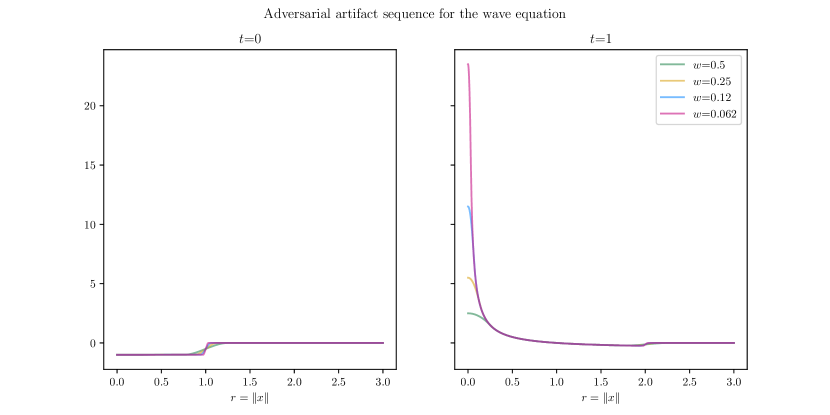
we verify that is a Fourier multiplier of the form (1) with , hence a bounded linear operator . However, it is simple to find bounded initial conditions that can become arbitrarily large in at time . For example, consider smooth radially symmetric initial conditions,
When evaluated at , the solution satisfies
(see e.g. Kirchhoff’s formula [26, §12]). Thus, by increasing the slope of at , we can increase the norm of . We construct an adversarial sequence (cf. Definition 2.1) relative to by setting, for all , with compactly supported and such that , , as well as . Then, we get
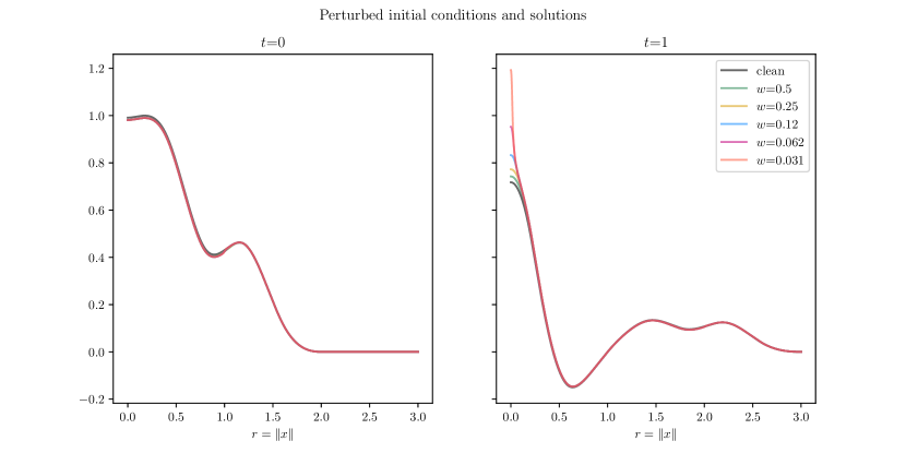
See Figure 1 for an example. Figure 2 shows such a sequence as perturbations to a signal of larger amplitude.
3.2 Filtering in space and frequency
In order to mitigate effects such as the adversarial sequences in Section 3.1, we can employ filters in both frequency and space to approximate .
Proposition 3.1.
Let and be two families of functions such that for all . Then the operator
is well defined and bounded for every . In particular,
Proof.
Straightforward computation, using Hölder’s inequality and the Plancherel theorem, gives
and further,
Therefore is bounded both as an operator and . By the Riesz-Thorin interpolation theorem it is therefore bounded as an operator for . ∎
One can, for example, take as filter the families
(where is the ball around the origin with radius ). The bounds above become
and
where is the volume of the unit ball in . We shall see that this choice is not optimal.
For certain families of filters, the operator can be written as a composition of with a preconditioning operator . This is highly beneficial for implementation if the multiplier is not known. Let us record some boundedness properties of this operator.
Lemma 3.2.
Let and be two families of functions such that for all , and for all . The linear operator
| (2) |
is well defined and bounded for , where
Proof.
By Young’s convolution inequality, we have
for , which shows that is bounded . Now, for we have
by applying Young’s convolution inequality again, together with Hölder’s inequality. This shows that is bounded as well. ∎
An interpretation of Lemma 3.2 is that for any , the operator is bounded and maps into the domain of the Fourier transform. In fact, a corollary of Lemma 3.2 is that is bounded for all .
Remark 3.3.
If with for all , then and we get
by the convolution theorem:
Note that Lemma 3.2, Hölder’s inequality, and the Hausdorff-Young inequality ensure that the Fourier transforms of and exist for for any . However, in this case, is continuous by the Riemann-Lebesgue lemma, so filters such as are excluded.
Theorem 3.4 (Pointwise approximation in ).
Let be two functions satisfying . Define the families and through dilation,
| (3) | ||||
| (4) |
Then, for every we have
and
Proof.
Note that . We have established that and that . Therefore
Using the triangle inequality, Young’s convolution inequality, and the fact that , we get
Since and form an approximation to the identity, we have
which concludes the proof. ∎
Remark 3.5.
We now turn to uniform approximation of by . This is not meaningful unless , and therefore we may only consider coming from some subspace of with this property. We let it suffice to study functions coming from the space
on which does indeed approximate .
Theorem 3.6 (Pointwise approximation in ).
Define the families and as in Theorem 3.4. Then, for any with we have
Proof.
First note that is a continuous function by the Riemann-Lebesgue lemma, and that
and hence
for almost every . Moreover, we have
for all , and since is integrable, we have
by the dominated convergence theorem.
Assuming for simplicity, we get:
Here we have used the fact that is an approximation to the identity. This concludes the proof. ∎
3.3 The wave equation: a numerical example
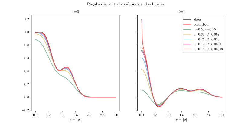
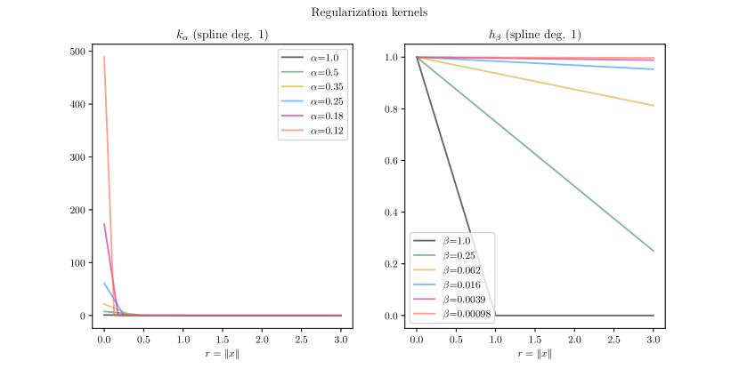
Having proved Theorems 3.4 and 3.6, we can confidently employ to tackle the adversarial sequences for wave propagation defined in Section 3.1. We make use of the decomposition , and choose simple radial filters,
which are shown in Figure 4 along with their dilations. Figure 3 shows the evolution of adversarially perturbed radial waves, as well as approximations by and .
4 Uniform approximation with spectral filtering and applications to inverse problems
In this section, will denote a compact linear operator between two separable Hilbert spaces with an infinite dimensional range. The space is otherwise arbitrary, but we will identify with for some measure space . We are interested in finding a regularization of the pseudoinverse that is also well behaved as an operator with the auxiliary space being .
As a compact operator, has a singular value decomposition
where and are orthonormal systems in and , respectively, and is a non-increasing sequence of positive real numbers with as . Likewise, the pseudoinverse can be expressed by
for
We make use of this fact heavily in what follows.
4.1 Instability in Tikhonov regularization
Consider the Tikhonov regularizer [8]
which can be expressed in terms of the SVD of as
This is a bounded operator as a mapping , with , but it is not, in general, bounded as a map for .
In the simplest case, the left singular vectors form an adversarial sequence for (cf. Definition 2.1). While they are bounded in (with norms equal to 1), we have
Therefore, for every , the sequence is bounded if and only if the sequence is bounded. In particular, if , then is not bounded from into . Further, if one of the right singular vectors is itself an unbounded function, then is not bounded from into .
This is only a necessary condition: there are situations where the sequence is bounded, but the Tikhonov regularizer is not bounded as an operator into . To see this, we consider the following example.
Example 4.1 (Periodic convolution).
Let , where is the unit circle (identified with ), and consider the periodic convolution operator defined for by
with some kernel . This operator is diagonal in the Fourier basis and its singular values are the absolute values of the non-zero Fourier coefficients of . Assuming, for ease of notation, that all Fourier coefficients of are non-zero, we thus obtain an SVD of with as right singular vectors, and a phase shifted version of the same basis as left singular vectors.
Suppose that the kernel is badly singular, so that , and that the (rearranged) singular values satisfy
with some . Define perturbations by
Since , we have , and hence the perturbations are bounded by .
Adversarial artifacts now appear at :
where for all . The perturbations form an adversarial sequence, and is an adversarial perturbation, namely, . Hence, is not bounded .
4.2 Spectral filtering
In order to ensure a bounded reconstruction into , we modify the Tikhonov regularizer by placing non-uniform weights in the SVD. That way, we can regularize more strongly in those directions that correspond to problematic right singular vectors.
Let be a sequence of real numbers that is bounded below by some positive number ,
Denote by the spectral filtering operator
| (5) |
The threshold ensures that this operator is dominated by a Tikhonov regularizer,
for all , and is thus bounded with
| (6) |
by Lemma A.1. The fact that will later be useful for obtaining a convergence rate for .
We remark that an alternative formulation of this operator is
where is the linear operator
defined on a subspace . With for all , we recover the familiar formulation of Tikhonov regularization.
Next, we show that spectral filtering is indeed a regularization method in , and that, under mild conditions, it converges in as well. Note that in order for it to be a regularization as an operator from to , we also need to establish that is bounded. This is the subject of Section 4.2.3.
4.2.1 Convergence
We now prove two approximation results: pointwise in for all and pointwise in under more restrictive assumptions. These theorems do not provide a convergence rate, as that will require more restrictions on .
Theorem 4.2 (Pointwise approximation in ).
We have
for all .
Proof.
Let . We will show that the error is smaller than for all smaller than some .
Since and by Picard’s criterion, we can select an integer large enough so that
and the error can be bounded as follows:
The result now follows by choosing small enough so that . ∎
Note that , and hence depends on , and the SVD of . As previously stated, we are interested in finding solutions to that lie in . Therefore, our regularization method should approximate uniformly whenever . Write
| (7) |
This is a subspace of , and is a somewhat stronger condition than , indeed
Similarly, if , then . We have the following convergence result, whose proof is similar to that of Theorem 4.2.
Theorem 4.3 (Pointwise approximation in ).
We have
for all .
Proof.
As before, we need to show that for any there exists some , such that for all
Since , we can select an integer large enough so that
The error can now be bounded as follows:
Choosing so that yields the result. ∎
4.2.2 Convergence rates on source sets
Theorems 4.2 and 4.3 provide no rate of convergence in terms of . In order to establish a convergence rate, we require some degree of “smoothness” of , something commonly known as a “source condition” in inverse problems [8]. Recall that the operator is assumed to be compact, so that as .
Definition 4.4.
Let . We say that satisfies the -strong Picard criterion if
| (8) |
Lemma 4.5.
Suppose that is a compact operator, and let . The set of elements of that satisfy the -strong Picard criterion,
forms a subspace of , and for any , we have
Proof.
For , and , we have
where we have used the triangle inequality and the basic fact that for any . This proves that is a subspace of .
Now let . Since is compact, we can find an such that for all . Then , so for , and therefore
In other words, implies , and therefore . ∎
Remark 4.6.
To establish rates of convergence for on the source sets, we follow a similar approach as in Chapter 4 of [8]. However, it needs to be adapted to the current case where the spectral filter does not depend exclusively on the singular values , but rather on their index . By imposing a condition on the growth of the coefficients relative to the decay of , standard proofs can be emulated. This comes at the cost of having to assume more smoothness of the data. Before we state the next convergence results, we need the following calculus fact.
Lemma 4.7.
Let and define the function by
If , then
for some , and if , then is strictly increasing.
Proof.
See Appendix A. ∎
Theorem 4.8 (Pointwise approximation in with convergence rate).
Suppose that is compact, and that the weights satisfy
| (9) |
for some . Let for some . Then there exists a constant , depending only on , , , and , such that
for all .
Proof.
Taking squared norms, we obtain
Now, we employ Lemma 4.7. If , then
and since , we have . If , then, by monotonicity of ,
Taking square roots on both sides of the above inequalities gives the result. ∎
Remark 4.9.
Next, we consider uniform approximation on the sets , . Again, we need a condition on the SVD of that relates the growth of to the decay of .
Lemma 4.10.
Proof.
Take . We use the triangle inequality and Hölder’s inequality for infinite series:
which is finite by (10) and using that . ∎
Remark 4.11.
Condition (10) significantly limits the choice for the parameter . For example, if , then is always at least 2 if the condition is to be satisfied. Consider a mildly ill-posed problem satisfying for some . Then
so (10) is satisfied if and only if . For severely ill-posed problems with , any suffices.
Theorem 4.12 (Pointwise approximation in with convergence rate).
Suppose that is compact and that its SVD satisfies
| (11) |
Moreover, suppose that the weights satisfy
for some . Let . Then there exists a constant such that
for all .
Proof.
We use the triangle inequality and rearrange exponents:
As in the proof of Theorem 4.8, we now use Lemma 4.7, by remarking that since the square root is an increasing function, has the same maxima as . For we get
The two norms are finite, because of (11) and using that for . For :
which, similarly, is finite because of (11) and ∎
4.2.3 Boundedness of the spectral filter
We now have a recipe for a spectral filtering operator that guarantees convergence both in and in , provided that certain conditions are satisfied. We have also noted at the beginning of this section, that this operator is bounded from into . However, for it to be indeed a regularization as an operator , we need to establish that it is (under certain conditions) a bounded operator with respect to these spaces. We assume that is compact, and that for all .
As for the convergence rate results, we will again suppose that for some , cf. (11). Under this condition, we can always find a sequence of weights such that is bounded.
Proposition 4.13.
Let be a compact operator with SVD such that for all and let (11) hold for some . If any lower bounded sequence of weights results in being bounded. If any choice with arbitrary constant implies boundedness of . In both cases,
for some independent of .
Proof.
If , for any
If choosing yields,
and we can similarly deduce that for all
By Lemma 4.10 and Theorem 4.3, in for all , and Theorem 4.12 provides a convergence rate for , as long as is such that
for some Thus, for the choice allows for any and for setting one can choose Therefore if , with appropriately chosen depending on and is the noise in the measurements with , we have
with the choice .
4.3 A numerical example
We revisit Example 4.1 to visualize the differences in approximation with and . The operator is a convolution with a singular kernel ,
for all . We choose a real valued kernel with
| (12) |
for . As shown in Example 4.1 (with ), this leads to a Tikhonov regularizer that admits adversarial perturbations.
The SVD of satisfies (11) for any . We choose weights for the modified regularizer according to Proposition 4.13, using ,
for . By Proposition 4.13, the resulting operator, is bounded and by Theorem 4.3 it is guaranteed to converge in to pointwise on the subspace from (7). By Theorem 4.12, we have
for and some constant .
We note that for any , the Sobolev space is a subspace of . Namely, there exist constants such that
for every and every . Likewise, we can characterize the source sets as follows:
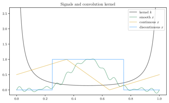
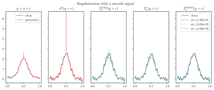
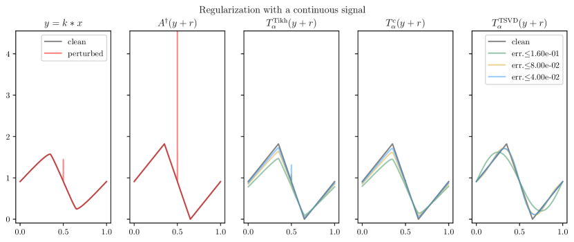
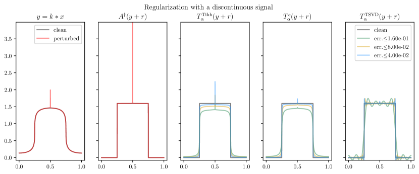
so for all .
Figure 5 shows the singular kernel along with signals satisfying three different smoothness criteria, and in Figures 6, 7, and 8, we show regularized solutions of . An adversarial perturbation is added to , which is constructed as explained in Example 4.1. We see that Tikhonov regularization struggles to suppress the resulting spike, while the effects are milder for . In addition, we show a truncated SVD approximation of the solution, , which can approximate smooth signals uniformly but is ill-suited for rough signals. In particular, the reconstruction in Figure 7 fails to well-approximate the corners at the points of no differentiability, and the reconstruction in Figure 8 suffers from the usual Gibbs phenomenon at the points of discontinuity. In both cases, the reconstructions provided by are superior in quality. It is worth observing that the discontinuous function of Figure 8 does not satisfy the assumptions of Theorem 4.3, and so uniform convergence is not guaranteed by the theory: it could serve as a motivation for extending the bounds obtained in this work to a larger class of functions.
Acknowledgements
We are happy to thank Fabio Nicola for useful discussions on specific examples for the wave equation. Co-funded by the European Union (ERC, SAMPDE, 101041040). Views and opinions expressed are however those of the authors only and do not necessarily reflect those of the European Union or the European Research Council. Neither the European Union nor the granting authority can be held responsible for them. This material is based upon work supported by the Air Force Office of Scientific Research under award numbers FA8655-20-1-7027 and FA8655-23-1-7083. Co-funded by the EU – Next Generation EU. The research was supported in part by the MIUR Excellence Department Project awarded to Dipartimento di Matematica, Università di Genova, CUP D33C23001110001. GSA is a member of the “Gruppo Nazionale per l’Analisi Matematica, la Probabilità e le loro Applicazioni”, of the “Istituto Nazionale di Alta Matematica”.
References
- Alaifari et al. [2019] R. Alaifari, G. S. Alberti, and T. Gauksson. ADef: an iterative algorithm to construct adversarial deformations. In Proceedings of the International Conference on Learning Representations (ICLR 2019), 2019.
- Alaifari et al. [2023] R. Alaifari, G. S. Alberti, and T. Gauksson. Localized adversarial artifacts for compressed sensing MRI. SIAM Journal on Imaging Sciences, 16(4):SC14–SC26, 2023.
- Antun et al. [2020] V. Antun, F. Renna, C. Poon, B. Adcock, and A. C. Hansen. On instabilities of deep learning in image reconstruction and the potential costs of AI. Proceedings of the National Academy of Sciences, 117(48):30088–30095, 2020.
- Biggio et al. [2013] B. Biggio, I. Corona, D. Maiorca, B. Nelson, N. Šrndić, P. Laskov, G. Giacinto, and F. Roli. Evasion attacks against machine learning at test time. In Joint European Conference on Machine Learning and Knowledge Discovery in Databases, pages 387–402, New York, 2013. Springer.
- Carlini and Wagner [2017] N. Carlini and D. Wagner. Towards evaluating the robustness of neural networks. In IEEE Symposium on Security and Privacy (SP), pages 39–57. IEEE, 2017.
- Chen et al. [2018] R. T. Q. Chen, Y. Rubanova, J. Bettencourt, and D. K. Duvenaud. Neural ordinary differential equations. In S. Bengio, H. Wallach, H. Larochelle, K. Grauman, N. Cesa-Bianchi, and R. Garnett, editors, Advances in Neural Information Processing Systems, volume 31. Curran Associates, Inc., 2018. URL https://proceedings.neurips.cc/paper_files/paper/2018/file/69386f6bb1dfed68692a24c8686939b9-Paper.pdf.
- E [2017] W. E. A proposal on machine learning via dynamical systems. Commun. Math. Stat., 5(1):1–11, 2017. ISSN 2194-6701,2194-671X. doi: 10.1007/s40304-017-0103-z. URL https://doi.org/10.1007/s40304-017-0103-z.
- Engl et al. [2000] H. W. Engl, M. Hanke, and A. Neubauer. Regularization of Inverse Problems. Kluwer Academic Publishers, Dordrecht, The Netherlands, 2000.
- Evans [2022] L. C. Evans. Partial differential equations, volume 19. American Mathematical Society, 2022.
- Genzel et al. [2022] M. Genzel, J. Macdonald, and M. März. Solving inverse problems with deep neural networks - robustness included. IEEE Transactions on Pattern Analysis and Machine Intelligence, 45(1):1119–1134, 2022. doi: 10.1109/TPAMI.2022.3148324.
- Goodfellow et al. [2016] I. Goodfellow, Y. Bengio, and A. Courville. Deep Learning. MIT Press, 2016. http://www.deeplearningbook.org.
- Goodfellow et al. [2014] I. J. Goodfellow, J. Shlens, and C. Szegedy. Explaining and harnessing adversarial examples. arXiv preprint arXiv:1412.6572, 2014.
- Gottschling et al. [2020] N. M. Gottschling, V. Antun, B. Adcock, and A. C. Hansen. The troublesome kernel: why deep learning for inverse problems is typically unstable. arXiv preprint arXiv:2001.01258, 2020.
- Haber and Ruthotto [2018] E. Haber and L. Ruthotto. Stable architectures for deep neural networks. Inverse Problems, 34(1):014004, 22, 2018. ISSN 0266-5611,1361-6420. doi: 10.1088/1361-6420/aa9a90. URL https://doi.org/10.1088/1361-6420/aa9a90.
- He et al. [2016] K. He, X. Zhang, S. Ren, and J. Sun. Deep residual learning for image recognition. In 2016 IEEE Conference on Computer Vision and Pattern Recognition (CVPR), pages 770–778, 2016. doi: 10.1109/CVPR.2016.90.
- Higham and Higham [2019] C. F. Higham and D. J. Higham. Deep learning: An introduction for applied mathematicians. SIAM Review, 61(4):860–891, 2019. doi: 10.1137/18M1165748. URL https://doi.org/10.1137/18M1165748.
- Kalton and Montgomery-Smith [2003] N. Kalton and S. Montgomery-Smith. Interpolation of Banach spaces. handbook of the geometry of Banach spaces, vol. 2, 1131–1175. North-Holland, Amsterdam, 164:165, 2003.
- Madry et al. [2018] A. Madry, A. Makelov, L. Schmidt, D. Tsipras, and A. Vladu. Towards deep learning models resistant to adversarial attacks. In International Conference on Learning Representations, 2018. URL https://openreview.net/forum?id=rJzIBfZAb.
- Moosavi-Dezfooli et al. [2016] S.-M. Moosavi-Dezfooli, A. Fawzi, and P. Frossard. Deepfool: a simple and accurate method to fool deep neural networks. In Proceedings of the IEEE conference on computer vision and pattern recognition, pages 2574–2582, 2016.
- Möbius [1994] P. Möbius. Dautray, r.; lions, j.-l., mathematical analysis and numerical methods for science and technology. vol.5: Evolution problems i. berlin etc., springer-verlag 1992. xiv, 709 pp., dm 198,oo. isbn 3-540-50205-x. ZAMM - Journal of Applied Mathematics and Mechanics / Zeitschrift für Angewandte Mathematik und Mechanik, 74(2):104–104, 1994. doi: https://doi.org/10.1002/zamm.19940740210. URL https://onlinelibrary.wiley.com/doi/abs/10.1002/zamm.19940740210.
- Peral [1980] J. C. Peral. estimates for the wave equation. Journal of Functional Analysis, 36(1):114–145, 1980. ISSN 0022-1236. doi: https://doi.org/10.1016/0022-1236(80)90110-X. URL https://www.sciencedirect.com/science/article/pii/002212368090110X.
- Ruthotto and Haber [2020] L. Ruthotto and E. Haber. Deep neural networks motivated by partial differential equations. Journal of Mathematical Imaging and Vision, 62(3):352–364, 2020. doi: 10.1007/s10851-019-00903-1. URL https://doi.org/10.1007/s10851-019-00903-1.
- Schuster et al. [2012] T. Schuster, B. Kaltenbacher, B. Hofmann, and K. S. Kazimierski. Regularization Methods in Banach Spaces. De Gruyter, Berlin, Boston, 2012. ISBN 9783110255720. doi: doi:10.1515/9783110255720. URL https://doi.org/10.1515/9783110255720.
- Sogge [1993] C. D. Sogge. estimates for the wave equation and applications. Journées équations aux dérivées partielles, pages 1–12, 1993.
- Szegedy et al. [2013] C. Szegedy, W. Zaremba, I. Sutskever, J. Bruna, D. Erhan, I. Goodfellow, and R. Fergus. Intriguing properties of neural networks. arXiv preprint arXiv:1312.6199, 2013.
- Vladimirov [1971] V. Vladimirov. Equations of Mathematical Physics. Marcel Dekker Inc., New York, New York, 1971.
- Xiao et al. [2018] C. Xiao, J.-Y. Zhu, B. Li, W. He, M. Liu, and D. Song. Spatially transformed adversarial examples. In International Conference on Learning Representations, 2018. URL https://openreview.net/forum?id=HyydRMZC-.
Appendix A Proofs
We collect here some proofs and auxiliary results.
Proof of Theorem 2.3. We assume that (i.e. no adversarial perturbation exists) and show that no adversarial sequence can exist.
The intersections and are Banach spaces when equipped with the norms
We show that the operator is bounded with respect to these norms by using the Closed Graph Theorem. Let be a sequence in the graph of ,
that converges to a point in the product norm
Since
we have
Since
we can see that the sequence converges to both and in . This means that , and hence . We have shown that is a closed subspace of , and thus that is bounded with respect to and .
The result now follows. Since
for all , any sequence in that is bounded in both and has a bounded image in and hence is not an adversarial sequence. ∎
The following is an adaptation of Theorem 4.2 from [8] for the specific case of Tikhonov regularization (for which the constant therein can be chosen equal to ).
Lemma A.1.
For all , we have
Proof.
Proof of Lemma 4.7. We derive:
This is strictly positive for . For , if and only if
which is a maximum (by straightforward calculation, ). We evaluate:
where ∎
Appendix B Connections to the stability of deep neural networks
In this appendix, we briefly discuss the link between feed-forward deep neural networks (DNN) and hyperbolic equations, and why the results of this paper can provide interesting insights for the study of the stability of DNNs.
Let us start by introducing DNNs; the reader is referred to [11, 16] for additional details on the basics of DNNs. A DNN is a function that can be written as a composition of layers:
where
| (13) |
Here, describes the action of the -th layer, and is a map parametrized by . We collect all the weights into a single vector , which is typically learned during training. The most common choice for is
where , is a bias term, and is a fixed nonlinearity, such as the rectified linear unit , acting pointwise. In the case when no additional structure is imposed on the weights, the free parameters are , and the network is called fully connected, because every node of the output is linked to every node in the input through the linear map . It is also possible to restrict the choice of the maps : for example, considering convolutions allows for a reduction in the number of free parameters, and yields translation invariant (often called equivariant) layers. An alternative to (13) was proposed in [15] in order to learn a perturbation of the identity only, namely
| (14) |
Here, for simplicity we consider only the case when all the dimensions coincide, and . This choice gives rise to the so-called residual neural networks (ResNets).
It is possible to view the discrete variable parametrizing the layers of a ResNet as a discretization of the continuous time of a dynamical system [7, 14, 6]. More precisely, (14) can be seen as the forward Euler step (with step size ) of the Cauchy problem
| (15) |
The output of the network is given by the solution at time , namely . Furthermore, we can view the vectors as discretizations of functions of two or three variables, modeling 2D and 3D signals, respectively. In this continuous settings, convolutions with filters with small support become differential operators [22]. As a consequence, the maps can be taken as certain, possibly nonlinear, differential operators, acting on the function , and (15) becomes an initial value problem for a PDE, called parabolic CNN in [22]. The simplest example in this setting is associated to , giving rise to the (linear) heat equation. Considering time/spatial-dependent, possibly nonlinear, differential operators with learnable parameters gives rise to more complicated evolutions.
Heat-type equations tend to dissipate energy. For energy preservation, it is natural to consider hyperbolic CNNs, which take the form
| (16) |
As above, the trivial choice corresponds to the (linear) wave equation with constant coefficients, and other choices give rise to more complicated, possibly nonlinear, hyperbolic PDEs.
The theoretical results of [22] show that both PDEs (15) and (16) have Lipschitz stability properties, in the sense that
for some . These estimates are useful in the context of stability of DNNs and, especially, for studying robustness against adversarial attacks, as discussed in Section 1. Indeed, they guarantee that the output of a neural network depends continuously (in fact, in a Lipschitz way) on the input, and they quantify this dependence by the constant . However, as we argue in Section 1, the norm may not capture all the relevant deformations of a signal. For instance, the norm is more suited to capture localized perturbations. The results of this paper, and especially those presented in Section 3 address this issue in the very simple setting of the linear wave equation: stability in does not hold in general, and a filtering approach is introduced to overcome this issue. Our approach does not directly apply to more complicated nonlinear settings, which are interesting for applications to neural networks, but can serve as an initial investigation on this issue.