pycvxset: A Python package for convex set manipulation

Abstract

This paper introduces pycvxset, a new Python package to manipulate and visualize convex sets. We support polytopes and ellipsoids, and provide user-friendly methods to perform a variety of set operations. For polytopes, pycvxset supports the standard halfspace/vertex representation as well as the constrained zonotope representation. The main advantage of constrained zonotope representations over standard halfspace/vertex representations is that constrained zonotopes admit closed-form expressions for several set operations. pycvxset uses CVXPY to solve various convex programs arising in set operations, and uses pycddlib to perform vertex-halfspace enumeration. We demonstrate the use of pycvxset in analyzing and controlling dynamical systems in Python. pycvxset is available at https://github.com/merlresearch/pycvxset under the AGPL-3.0-or-later license, along with documentation and examples.

I Introduction

Set-based methods provide a formal framework to analyze and control dynamical systems. Such methods are often used in set propagation and reachability analysis where the goal is to characterize system states and a family of controllers with some desirable properties [1, 2, 3, 4]. For example, in spacecraft rendezvous, we can use set-based methods to define a range of acceptable positions and velocities along the nominal spacecraft trajectory to ensure a safe abort when needed [5, 6, 7]. See [3, 1, 8, 9, 10] for other applications of set-based control methods.

For linear systems, set-based methods yield practical implementations using efficient set representations like ellipsoids and polytopes. However, several set operations are not closed in ellipsoids [11], and certain set operations in the standard vertex/halfspace representation of polytopes require computationally expensive vertex-halfspace enumeration [3]. Recently, constrained zonotopes have been proposed for performing exact set operations on polytopes, since 1) they provide an equivalent representation of polytopes, and 2) they allow for closed-form expressions for several set operations [8, 9, 6, 7, 10].

Several open-source software toolboxes implement some or all of these set representations and their operations in various languages [12, 13, 14, 15, 16, 17, 18, 11]. Together, these toolboxes have been instrumental in improving the access to set-based methods for reachability and trajectory optimization for the broader dynamical systems and control community. While existing tools in Python [12, 13, 14, 15] have primarily focused on polytopes, MATLAB tools [16, 17, 18, 11] are more mature and accommodate more set representations. pycvxset aims to help bridge this gap.

This paper introduces pycvxset, a Python package to manipulate and visualize convex sets. With pycvxset, we hope to bring the recent progress made in set representations especially constrained zonotopes [7, 8, 9, 6] to Python. pycvxset extends pytope [13] to include ellipsoidal and constrained zonotopic set representations, broaden the capabilities of Polytope class including 3D plotting, and integrates with CVXPY for use in constrained control. pycvxset is extensively tested and documented for reliability and ease of use.

II Set representations and operations

II-A Set representations

We briefly review the various set definitions supported by pycvxset. We say two set representations are equivalent when the sets they represent contain each other. Note that pycvxset only supports bounded sets.

From [3, 8], the following three set representations are equivalent:

$$\mathcal{P}(V) =\left\{x\in\mathbb{R}^{n}\ \middle|\begin{array}[]{c}\exists\theta\in\mathbb{R}^{N},\ x=V^{\top}\theta\\ 1^{\top}\theta=1,\ \theta\geq 0\end{array}\right\},$$ (3)

$$\mathcal{P}(A,b,A_{e},b_{e}) =\{x\in\mathbb{R}^{n}\ |\ Ax\leq b,\ A_{e}x=b_{e}\},$$ (4)

$$\mathcal{P}(G,c,A_{e},b_{e}) =\left\{x\in\mathbb{R}^{n}\middle|\begin{array}[]{c}\exists\xi\in\mathbb{R}^{N},\ x=G\xi+c,\\ \|\xi\|_{\infty}\leq 1,\ A_{e}x=b_{e}\end{array}\right\},$$ (7)

with appropriate dimensions for $V,A,b,A_{e},b_{e},G,c$. Specifically, (3) is the vertex representation, (4) is the halfspace representation, and (7) is the constrained zonotopic representation of a polytope. While the equivalence of (3) and (4) is well-known [3], the equivalence to a constrained zonotope representation was recently established in [8, Thm. 1].

The following sets are special cases of polytopes:

$$\mathcal{R}(l,u) =\{x\in\mathbb{R}^{n}\ |\ l\leq x\leq u\}$$ (8)

$$\mathcal{R}(c,h) =\{x\in\mathbb{R}^{n}\ |\ \forall i\in\{1,2,\ldots,n\},\ |x_{i}-c_{i}|\leq h_{i}\}$$ (9)

$$\mathcal{Z}(G,c) =\{x\in\mathbb{R}^{n}\ |\ \exists\xi\in\mathbb{R}^{N},\ x=G\xi+c,\ \|\xi\|_{\infty}\leq 1\}.$$ (10)

for finite vectors $l,u,c,h\in\mathbb{R}^{n}$ and appropriately dimensioned matrix $G$. Here, (8) and (9) represent axis-aligned rectangles, and (10) represents zonotopes.

Throughout this paper, we refer to sets represented in the form of (3) and (4) as polytopes and those in the form of (7) as constrained zonotopes, even though they all represent the same set [8, 9, 6]. We refer to unbounded sets of the form (4) as polyhedra.

Finally, we consider ellipsoidal sets $\mathcal{E}$ (11)–(13):

$$\mathcal{E}(Q,c) =\{x\in\mathbb{R}^{n}\ |\ {(x-c)}^{\top}Q(x-c)\leq 1\}$$ (11)

$$\mathcal{E}(G,c) =\{x\in\mathbb{R}^{n}\ |\ \exists\xi\in\mathbb{R}^{n},\ x=G\xi+c,\ \|\xi\|_{2}\leq 1\}$$ (12)

$$\mathcal{B}(c,r) =\{x\in\mathbb{R}^{n}\ |\ {\|x-c\|}_{2}\leq r\}.$$ (13)

Here, the set representations (11) and (12) are equivalent [19], and (13) is a $n$-dimensional ball.

II-B Set operations

For any sets $\mathcal{T},\mathcal{S}\subseteq\mathbb{R}^{n}$ and $\mathcal{W}\subseteq\mathbb{R}^{m}$, and a matrix $R\in\mathbb{R}^{m\times n}$, we define the set operations (affine map, Minkowski sum $\oplus$, intersection with inverse affine map $\cap_{R}$, and Pontryagin difference $\ominus$):

$$R\mathcal{T} \triangleq\{Ru:u\in\mathcal{C}\},$$ (14a)

$$\mathcal{T}\oplus\mathcal{S} \triangleq\{u+v:u\in\mathcal{C},\ v\in\mathcal{S}\},$$ (14b)

$$\mathcal{T}\cap_{R}\mathcal{W} \triangleq\{u\in\mathcal{C}:Ru\in\mathcal{W}\},$$ (14c)

$$\mathcal{T}\ominus\mathcal{S} \triangleq\{u:\forall v\in\mathcal{S},u+v\in\mathcal{C}\}.$$ (14d)

Since $\mathcal{C}\cap\mathcal{S}=\mathcal{C}\cap_{I_{n}}\mathcal{S}$, (14c) also includes the standard intersection. For any $x\in\mathbb{R}^{n}$, we use $\mathcal{C}+x$ and $\mathcal{C}-x$ to denote $\mathcal{C}\oplus\{x\}$ and $\mathcal{C}\oplus\{-x\}$ respectively for brevity. The set operations (14) can also be used to define several other operations like orthogonal projection and inverse affine transformation (see Table I), and slicing (an intersection with an axis-aligned affine set).

The key advantage of constrained zonotopes over polytopes is that they admit closed form expressions for all set operations listed in (14) (except Pontryagin difference (14d)) [8, 9]. Recently, the authors have proposed a closed-form expression to inner-approximate the Pontryagin difference (14d) [6]. In contrast, polytopes must contend with computationally expensive vertex-halfspace enumeration when certain set operations are performed on a polytope in vertex/halfspace representation.

III The pycvxset package

pycvxset provides three classes for representing convex sets (3)–(13): Polytope, ConstrainedZonotope, and Ellipsoid. In this section, we provide a brief overview of how we use pycvxset to define, manipulate, and visualize these sets in Python.

III-A Set definitions

III-A1 Polytope

We define a set in polytopic representation using the Polytope class in the following ways:
1) specifying $(V)$ to define a polytope in V-Rep (3),
2) specifying $(A,b)$ or $(A,b,Ae,be)$ to define a polytope in H-Rep (4), and
3) specifying rectangles $(l,u)$ (see (8)) or $(c,h)$ (see (9)). We also provide methods to convert a polytope from vertex representation to half-space representation and vice versa using pycddlib and scipy.

The following code snippet creates a polytope in V-Rep and $3$-dimensional simplex in H-Rep, prints the description of the polytope along with its vertices.

⬇

1import numpy as np

2from pycvxset import Polytope

3

4V = [[-1,0.5],[-1,1],[1,1],[1,-1],[0.5,-1]]

5P1 = Polytope(V=V)

6print("P1 is a", repr(P1))

7A, b = -np.eye(3), np.zeros((3,))

8Ae, be = [1, 1, 1], 1

9P2 = Polytope(A=A, b=b, Ae=Ae, be=be)

10print("P2 is a", P2)

11print("Vertices of P2 are:\n", P2.V)

12print("P2 is a", P2)

The above code snippet produces the following output:

⬇

P1 is a Polytope in R^2 in only V-Rep

In V-rep: 5 vertices

P2 is a Polytope in R^3 in only H-Rep

Vertices of P2 are:

[[0. 0. 1.]

[0. 1. 0.]

[1. 0. 0.]]

P2 is a Polytope in R^3 in H-Rep and V-Rep

The call P2.V in Line 11 triggers a vertex enumeration internally as seen from the print statements for P2.

III-A2 Constrained zonotope

We define a set in constrained zonotopic representation (7) using the ConstrainedZonotope class in the following ways:
1) specifying $(c,G,Ae,be)$ as given in (7),
2) specifying $(c,G)$ as given in (10) to define a zonotope,
3) specifying a Polytope object (3), (4), and
4) specifying rectangles $(l,u)$ (see (8)) or $(c,h)$ (see (9)).

The following code snippet creates a constrained zonotope from the polytope defined before as well as a box.

⬇

1from pycvxset import ConstrainedZonotope

2

3C1 = ConstrainedZonotope(polytope=P1)

4print("C1 is a", repr(C1))

5print("P1 is a", repr(P1))

6C2 = ConstrainedZonotope(lb=[-1, -1], ub=[1, 1])

7print("C2 is a", repr(C2))

The above code snippet produces the following output:

⬇

C1 is a Constrained Zonotope in R^2

with latent dimension 7 and 5 equality constraints

P1 is a Polytope in R^2 in H-Rep and V-Rep

In H-rep: 5 inequalities and no equality constraints

In V-rep: 5 vertices

C2 is a Constrained Zonotope in R^2

that is a zonotope with latent dimension 2

pycvxset performs a halfspace enumeration for P1 (currently in vertex representation) in order to generate a constrained zonotopic representation (7) using [8, Thm. 1]. pycvxset also detects that C2 is a zonotope.

pycvxset provide methods to generate polytopic approximations of constrained zonotopes (see Section III-B). Due to the computational effort involved [8], an exact conversion from (7) to (3) or (4) is not supported.

III-A3 Ellipsoid

We define an ellipsoid using the Ellipsoid class in the following ways:
1) specifying $(Q,c)$ as given in (11),
2) specifying $(G,c)$ as given in (12), and
3) specifying $(c,r)$ to define a ball (13).

pycvxset currently supports only ellipsoids with positive definite $Q$, i.e., full-dimensional ellipsoids (see [19]). The following code snippet creates two ellipsoids of the forms (11) and (12).

⬇

1from pycvxset import Ellipsoid

2

3E1 = Ellipsoid(c=[2,-1], Q=np.diag([1,4]))

4print("E1 is an", E1)

5E2 = Ellipsoid(c=[0,1,0], G=np.diag([1,2,3]))

6print("E2 is an", E2)

The above code snippet produces the following output:

⬇

E1 is an Ellipsoid in R^2

E2 is an Ellipsoid in R^3

III-B Visualizing polytopes and polytopic approximations

We plot 2D and 3D polytopes using pycvxset and matplotlib, and plot polytopic approximations of constrained zonotopes and ellipsoids (see Fig. 1).

The following code snippet plots the sets in Fig. 1.

⬇

1import matplotlib.pyplot as plt

2

3plt.figure()

4ax = plt.subplot(131, projection="3d")

5P2.plot(ax=ax) # Plot polytope

6ax.view_init(elev=30, azim=-15)

7ax.set_aspect("equal")

8ax.set_title("Polytope")

9ax = plt.subplot(132) # Plot const. zonotope

10C1.plot(ax=ax, vertex_args={"visible": True})

11ax.set_aspect("equal")

12ax.set_title("Constrained Zonotope")

13ax = plt.subplot(133) # Plot ellipsoid

14E1.plot(ax=ax,patch_args={"facecolor":"pink"})

15ax.set_aspect("equal")

16ax.set_title("Ellipsoid")

17plt.subplots_adjust(wspace=0.5)

Figure 1: Plotting various sets using pycvxset.

pycvxset provides flexibility in plotting either faces, vertices, or both, and provides identical methods for plotting irrespective of the set representation. By default, pycvxset plots inner-approximations of constrained zonotopes and ellipsoids, but outer-approximations may be plotted when required. For brevity, we will omit plotting commands in subsequent code snippets.

We compute polytopic inner- and outer-approximations for ellipsoids and constrained zonotopes of any $n$-dimensional set using their support function and support vectors. While pycvxset accepts user-specified directions, it can also autogenerate well-separated $2n+2^{n}D$ direction vectors for any $D\in\mathbb{N}$, by solving the following optimization problem [20, Eq. (B.1)],

$$\begin{array}[]{rll}\text{max.}&r\\ \text{s.\ t.}&{\|x_{i}-x_{j}\|}_{2}\geq r,&\forall 1\leq i<j\leq D,\\ &{\|x_{i}-e_{j}\|}_{2}\geq r,&\forall 1\leq i\leq D,\ \forall 1\leq j\leq n,\\ &2x_{i}\geq r,\ 0.8\leq\|x_{i}\|\leq 1,&\forall 1\leq i\leq D.\\ \end{array}$$ (19)

Here, the decision variables are vectors $x_{i}\in\mathbb{R}^{n}$ for $i\in\{1,2,\ldots,D\}$ and a scalar $r$, and $e_{j}$ denotes the standard axis vector in $\mathbb{R}^{n}$. (19) is a difference-of-convex program that aims to spread points $x_{i}$ on the intersection of a unit sphere and the positive quadrant $\mathbb{R}_{\geq 0}^{n}$, which are subsequently reflected the axis planes to yield the direction vectors [20, 21]. (19) may be solved (approximately) via the well-known convex-concave procedure [22], and the approach is implemented in pycvxset as the method spread_points_on_a_unit_sphere. pycvxset uses $D=20$ as the default value. Fig. 2 shows the result of (19) for $n=3$.

Figure 2: Well-separated vectors on a $3$-dimensional unit sphere.

III-C Set operations

TABLE I: pycvxset set operations on a set $X\subset\mathbb{R}^{n}$. Here, ✓ indicates exact implementation, $\dagger$ indicates exact implementation possible after converting Polytope to ConstrainedZonotope, and $\approx$ indicates approximate implementation. All operations for constrained zonotopes and ellipsoids may be approximated, if desired, using appropriate polytopic approximations.

Operation Expression Polytope Constrained Ellipsoid zonotope Set computations involving another vector $v$ and/or matrix $M$ Affine transformation $(M,v)$ for $M\in\mathbb{R}^{m\times n},v\in\mathbb{R}^{m}$ $MX+v$ ✓ ✓ ✓ ($M$ full row-rank) Inverse-affine transformation $M\in\mathbb{R}^{n\times n}$, $M$ is invertible $\{x\ |\ Mx\in X\}$ ✓ ✓ ✓ Project a point $v\in\mathbb{R}^{n}$ on to $X$ using ${\|\cdot\|}_{p}$, $p\in\{1,2,\infty\}$ $\arg\min_{x\in X}\|x-v\|_{p}$ ✓ ✓ ✓ Containment of a point $v\in\mathbb{R}^{n}$ in $X$ $v\in X$ ✓ ✓ ✓ Support function along a direction $v\in\mathbb{R}^{n}$ $\sup_{x\in X}v^{T}x$ ✓ ✓ ✓ Support vector along a direction $v\in\mathbb{R}^{n}$ $\arg\sup_{x\in X}v^{T}x$ ✓ ✓ ✓ Centering Chebyshev center $\sup_{\mathrm{Ball}(x,r)\subseteq X}\ r$ ✓ subopt. $\approx$ ✓ Maximum volume inscribed ellipsoid $\sup_{\mathcal{E}(c,Q)\subseteq X}\ \mathrm{Vol}(\mathcal{E})$ ✓ subopt. $\approx$ ✓ Minimum volume circumscribed ellipsoid $\inf_{\mathcal{E}(c,Q)\supseteq X}\ \mathrm{Vol}(\mathcal{E})$ ✓ ✓ Minimum volume circumscribed rectangle $\inf_{\mathrm{Rect}(l,u)\supseteq X}\ \mathrm{Vol}(\mathrm{Rect})$ ✓ ✓ ✓ Other set-specific manipulations/computations Interior point (Relative) Compute $x\in X$ ✓ ✓ ✓ Orthogonal projection to $\mathbb{R}^{m}$ $\{x|\exists v\in\mathbb{R}^{n-m},\ [x;v]\in X\}$ ✓ ✓ ✓ Volume $\mathrm{Vol}(X)$ ✓ $\approx$ ($n=2$) ✓ Set computations involving another set $Y$ ($Y\subset\mathbb{R}^{n}$ unless specified otherwise) Intersection with a polytope $Y$ $X\cap Y$ ✓ ✓ Intersection with a constrained zonotope $Y$ $\dagger$ ✓ Intersection with an affine set $Y$ ✓ ✓ Intersection with a polyhedron $Y$ ✓ ✓ Intersection with $Y\subset\mathbb{R}^{m}$ under inverse affine map $M\in\mathbb{R}^{m\times n}$ $X\cap_{M}Y=\{x\in X|Mx\in Y\}$ ✓ ✓ Minkowski sum with a polytope $Y$ $X\oplus Y$ ✓ ✓ Minkowski sum with a constrained zonotope $Y$ $\dagger$ ✓ Pontryagin difference with an ellipsoid $Y$ $X\ominus Y$ ✓ inner $\approx$ Pontryagin difference with a zonotope $Y$ ✓ inner $\approx$ Pontryagin difference with a polytope $Y$ ✓ Containment of a polytope $Y$ $Y\subseteq X$ ✓ ✓ ✓ Containment of a constrained zonotope $Y$ ✓ ✓ Containment of an ellipsoid $Y$ ✓ ✓

Table I lists the set operations supported for each class. pycvxset provides identical methods for various set operations (when supported).

III-C1 Involving another vector $v$ and/or matrix $M$

For any set $X$, we support affine transformation $(M,v)$, inverse-affine transformation with invertible map $M$, projecting a point $v$, checking if $v\in X$, and computing the support function and vector of the set $X$ along the direction $v$. We require inverse-affine map to have an invertible $M$ to ensure that the pre-image of a bounded set under the affine map $M$ is also bounded. For an affine transformation of an ellipsoid, we require $M$ used to have full row-rank to guarantee full-dimensionality of the image ellipsoid [11]. These operations either have a closed-form expressions (e.g., affine transformation of constrained zonotope [8] or support function of an ellipsoid [11]) or require solving convex programs which we implement using CVXPY (e.g., checking $v\in X$ for a polytope $X$ is a linear program).

As an illustration, we compute the Euclidean projection and the distance of a point $[1,1,1]$ on the polytope P2 using the following code snippet (see Fig. 3).

⬇

1point = np.array([1, 1, 1])

2projection, d = P2.project(point, p=2)

Figure 3: Projection of a point on a polytope

III-C2 Centering

Centering methods provide a succinct, approximate representation of complex sets in the form of ellipsoids and rectangles [19, Ch. 8]. These methods solve convex programs for polytopes in V-Rep/H-Rep, and are available in closed-form for ellipsoids [11]. For constrained zonotopes, we provide approximations [7].

Fig. 4 illustrates centering and bounding sets for the polytope P1 and the constrained zonotope C1. We obtained Chebyshev radius and ellipsoids of volume of $0.73$ and $1.89$ for P1 and $0.68$ and $1.81$ for C1 respectively, and obtained identical rectangles.

Figure 4: Centering for a polytope and a constrained zonotope.

III-C3 Other set-specific manipulations/computations

We use centering techniques for the computation of an interior point for each set. For polytopes, we can also compute its centroid (the mean of its vertices) as an alternative.

We compute the orthogonal projection of a set using an appropriately defined affine map.

We compute the projection of a $3$-dimensional unit $\ell_{1}$-norm ball using the following code snippet (see Fig. 5). Note that pycvxset counts dimensions from zero.

⬇

1V = np.vstack((np.eye(3), -np.eye(3)))

2l1ball = Polytope(V=V)

3ball2D = l1ball.projection(project_away_dim=2)

Figure 5: Projection of a $3$-dimensional unit $\ell_{1}$-norm ball.

We compute the volume of a full-dimensional polytope and an ellipsoid using scipy and closed-form expressions respectively. We approximate the volume of a constrained zonotope via grid-based sampling.

III-C4 Involving another set $Y$

We provide exact implementations for intersection and Minkowski sum of polytopes and constrained zonotopes among themselves, and for Pontryagin difference of polytopes with any other sets [23]. The intersection and Minkowski sum of a constrained zonotope and a polytope returns a constrained zonotope. The Pontryagin difference of a constrained zonotope and an ellipsoid or a zonotope is inner-approximated with a constrained zonotope using least squares [6].

We implement an exact check for the containment of a polytope $Y$ within a set $X$ (not necessarily a polytope) by solving appropriate convex programs [19], where we check for the containment of all the vertices of $Y$ in the set $X$. We also implement an exact check for the containment of a set $Y$ (not necessarily a polytope) within a polytope $X$ using the support function [19]. We implement an exact check for the containment of an ellipsoid in another ellipsoid using semi-definite programming [19].

To implement exact check for $Y\subseteq X$ for two constrained zonotopes $X,Y$, we encode $x\in Y\Rightarrow x\in X$ as a bilinear program obtained using strong duality:

$$\begin{array}[]{rl}\text{minimize}&1+\alpha^{\top}(c_{Y}-G_{X}\xi_{X}-c_{X})-\beta^{\top}b_{e,Y}\\ \text{subject\ to}&\|\xi_{X}\|_{\infty}\leq 1,\\ &A_{e,X}\xi=b_{e,X},\\ &{\|G_{Y}^{\top}\alpha+A_{e,Y}^{\top}\beta\|}_{1}\leq 1.\end{array}$$ (24)

with decision variables $\alpha\in\mathbb{R}^{n},\beta\in\mathbb{R}^{M_{Y}},\xi_{X}\in\mathbb{R}^{N_{X}}$, and $Y\subseteq X$ if and only if the optimal value of (24) is non-negative. We solve (24) to optimality using CVXPY and GUROBI, and can also check for containment of polytopes within constrained zonotopes. These methods also enable checking for equality between polytopes and constrained zonotopes, as illustrated in the following code snippet.

⬇

1print(’C1 is a’, C1)

2print(’P1 is a’, P1)

3print(’Are C1 and P1 equal?’, C1 == P1)

4lb, ub, p, q = [-1, -1], [1, 1], [-1,-1], 0.5

5P1a = Polytope(lb=lb, ub=ub).intersection_with_halfspaces(A=p, b=q)

6C1a = ConstrainedZonotope(lb=lb, ub=ub).intersection_with_halfspaces(A=p, b=q)

7print(’C1a is a’, C1a)

8print(’P1a is a’, P1a)

9print(’Are P1 and P1a equal?’, P1a == P1a)

10print(’Are C1 and C1a equal?’, C1 == C1a)

The above code snippet produces the following output:

⬇

C1 is a Constrained Zonotope in R^2

P1 is a Polytope in R^2 in H-Rep and V-Rep

Are C1 and P1 equal? True

C1a is a Constrained Zonotope in R^2

P1a is a Polytope in R^2 in only H-Rep

Are P1 and P1a equal? True

Are C1 and C1a equal? True

The equality of the sets C1 and P1 may also be visually confirmed in Fig. 4, where the polytopic inner-approximation of C1 computed by pycvxset for plotting is exact for this constrained zonotope instance. In contrast to the sets P1 and C1 defined in Sections III-A1 and III-A2, the sets P1a and C1a defined in Lines 5 and 6 in the above code snippet are defined by an intersection of a unit $\ell_{\infty}$-norm ball and an appropriate halfspace $\{x:p^{\top}x\leq q\}$. As expected, pycvxset declares all these sets to be equal, despite being different representations.

We support intersection of Polytope and ConstrainedZonotope objects with unbounded sets like affine sets and polyhedron since these operations are also closed in Polytope and ConstrainedZonotope respectively. We also implement slice using intersection with an appropriately-defined affine set.

We do not support intersection, Minkowski sum, and Pontryagin difference operations for ellipsoids natively in pycvxset since they are not closed operations for ellipsoids. However, all set operations discussed here are supported by Polytope. Consequently, any set operation that is not natively supported by pycvxset involving constrained zonotopes and ellipsoids may be approximated using their appropriate polytopic approximations (Section III-B). In Table I, ✓ indicates implementations of set operations in pycvxset that yields an object of the same class as $X$ and does not rely on polytopic approximations.

III-D Overloaded operators

We overload several Python operators to simplify the use of pycvxset. Table II summarizes how these operators interact with the sets in pycvxset.

When the comparison operators (<,<=,>,>=,in) are given a vector $y\in\mathbb{R}^{n}$ instead of a set $Y\subset\mathbb{R}^{n}$, pycvxset automatically switches to appropriate containment check with the vector $y$. Similarly, when the addition/subtraction operator is given a vector $y\in\mathbb{R}^{n}$, $X+y$, $y+X$, and $X-y$ translates $X$ by $y$, $y$, and $-y$ respectively.

We also support the operation of Cartesian product of a Polytope or a ConstrainedZonotope with itself.

TABLE II: Examples of python expressions involving sets $X,Y\subset\mathbb{R}^{n}$ defined from pycvxset, and an appropriate matrix $M$

Python expression Interpretation M * X, M @ X Affine map with $M\in\mathbb{R}^{m\times n}$ -X Negation, equivalent to -np.eye(X.dim) @ M X * M, X @ M Inverse affine map with invertible $M\in\mathbb{R}^{n\times n}$ X < Y, X <= Y, X in Y $X\subseteq Y$ X > Y, X >= Y, Y in X $X\supseteq Y$ X == Y Equality check — $X\subseteq Y$ and $Y\subseteq X$ X + Y Minkowski sum of $X$ with set $Y$ X - Y Pontryagin difference of $X$ with set $Y$ X ** m Cartesian product with itself $m\in\mathbb{N}$ times

III-E Solving relevant optimization problems

We use CVXPY to solve various optimization problems within pycvxset. We also provide methods to set up and solve convex programs with CVXPY involving sets constructed using pycvxset:
1) minimize to set up and solve optimization problems,

$$\begin{array}[]{rl}\text{minimize}&J(x),\\ \text{subject\ to}&x\in X,\\ \end{array}$$ (27)

for any CVXPY-compatible cost function $J$, and
2) containment_constraints to obtain the CVXPY expressions that enforce the containment constraints $x\in X$ as well as any necessary auxiliary variables.
Various methods in pycvxset like project, support use these methods to solve convex programs.

The user can specify the solver to use during set computations via the attributes cvxpy_args_lp, cvxpy_args_socp, and cvxpy_args_sdp associated with each object. These attributes are used when solving the various linear programs, second-order cone programs, and semi-definite programs respectively.

III-F Installation and examples

The source code of pycvxset along with detailed documentation and OS-specific installation instruction are available at https://github.com/merlresearch/pycvxset. We have tested pycvxset in Windows, Ubuntu, and MacOS, and for Python versions from 3.9 to 3.12. In future, we plan to register pycvxset to the Python Package Index as well. pycvxset is released under the AGPL-3.0-or-later license.

Additionally, we provide several Jupyter notebooks in the folder examples/ to help a user understand the different functionalities of pycvxset. We also provide a diagnostic script pycvxset_diag.py, which can help in checking if pycvxset was installed properly. Fig. 6 shows the results of running the command
$ python examples/pycvxset_diag.py
from the root of the package.

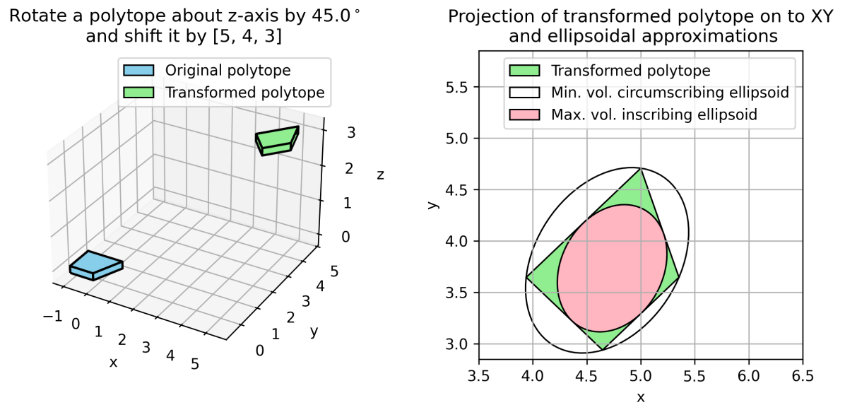
Figure 6: Figure generated by the script pycvxset_diag.py.

IV Reachability analysis using pycvxset

We now briefly discuss how pycvxset may be used to compute robust controllable (RC) sets [3, Defn. 10.18]. Consider a discrete-time linear time-invariant system with additive uncertainty,

$$x_{t+1}=Ax_{t}+Bu_{t}+Fw_{t},$$ (28)

with state $x_{t}\in\mathbb{R}^{n}$, input $u_{t}\in\mathcal{U}\subset\mathbb{R}^{m}$, disturbance $w_{t}\in\mathcal{W}\subset\mathbb{R}^{p}$, and appropriate matrices $A,B,F$. We assume that the input set $\mathcal{U}$ and disturbance set $\mathcal{W}$ are convex and compact sets. Given a horizon $N\in\mathbb{N}$, a polytopic safe set $\mathcal{S}\subset\mathbb{R}^{n}$ and a polytopic target set $\mathcal{T}\subset\mathbb{R}^{n}$, a $N$-step robust controllable set is the set of initial states that can be robustly driven, through a time-varying control law, to the target set in $N$ steps, while satisfying input and state constraints for all possible disturbances. Formally, we define the $N$-step RC set as $\mathcal{K}_{0}$ via the following set recursion for $t\in\{0,1,\ldots,N-1\}$:

$$\mathcal{K}_{t}=\mathcal{S}\cap\left({A^{-1}{((\mathcal{K}_{t+1}\ominus F\mathcal{W})\oplus(-B\mathcal{U}))}}\right),$$ (29)

with $\mathcal{K}_{N}\triangleq\mathcal{T}$. We implement (29) in pycvxset with the following Python function get_rcs.

⬇

1def get_rcs(S_U, S_W, S_S, S_T, A, B, F, N):

2 S_K = [None] * (N + 1)

3 S_K[-1], S_FW, S_BU = S_T, F@S_W, (-B)@S_U

4 for t in range(N - 1, -1, -1):

5 S_temp = (S_K[t+1] - S_FW) + S_BU

6 S_K[t]=S_S.intersection(S_temp @ A)

7 return S_K[0]

In get_rcs, we highlight variables denoting sets with a prefix S_ to distinguish from other variables — the horizon $N$ and matrices $A,B,F$ defined in (28). Here, S_U is $\mathcal{U}$, S_W is $\mathcal{W}$, S_T is $\mathcal{T}$, and S_S is $\mathcal{S}$.

Lines 2 and 3 of get_rcs initialize the sets and pre-compute the affine-mapped sets in (29). Lines 5-6 implement the set recursion (29) using Table II. The returned set S_K[0] is a ConstrainedZonotope (or a Polytope) when sets S_U, S_T, and S_S are ConstrainedZonotope (or Polytope) objects. For a ConstrainedZonotope-based computation, the set S_W must be a zonotope or an ellipsoid [6], while the set S_W can be any set in pycvxset for the Polytope-based computation (see Table I).

V Numerical examples

We provide several numerical examples to demonstrate various features of pycvxset. All computations were done on a standard laptop with 13th Gen Intel i7-1370P, 20 cores, 64 GB RAM using Python 3.9.

V-A Reachability analysis for a double integrator

We use pycvxset to compute a $30$-step RC set for a double integrator system model. A double integrator system can model an acceleration-controlled, mobile robot constrained to travel on a line. The corresponding RC set indicates the safe initial states that allow for subsequent satisfaction of state and input constraints. Using a sampling time of $0.1$, we have (28) with,

$$A=\left[\begin{array}[]{cc}1&0.1\\ 0&1\\ \end{array}\right],\ B=F=\left[\begin{array}[]{cc}0.005\\ 0.1\\ \end{array}\right],$$ (34)

with two-dimensional state $x_{t}$ denoting the position and velocity with one-dimensional input $u_{t}\in\mathcal{U}=[-1,1]$ and disturbance $w_{t}\in\mathcal{W}=0.4\times\mathcal{U}$ denoting the controlled acceleration and the perturbation. We choose the safe set $\mathcal{S}=[-1,1]\times[-0.5,0.5]$, which serves as position and velocity bounds the robot must satisfy at all times. We choose the target set $\mathcal{T}=[-0.25,0.25]\times[-0.1,0.1]$, which requires the robot to have a terminal position (at time $t=30$) within $0.25$ m of the origin, and a terminal velocity magnitude of at most $0.1$ m/s.

Fig. 7 shows the RC sets computed using get_rcs. Observe that the RC set computed using constrained zonotope is slightly smaller than the set computed using polytopes, due to the inner-approximation used in Pontryagin difference [6]. The overall computation time to generate and plot Fig. 7 was less than $3$ seconds.

Figure 7: $30$-step RC sets for (34) using pycvxset.

V-B Reach-avoid computation for spacecraft rendezvous

We now demonstrate a practical application of pycvxset where ConstrainedZonotope class provides scalability and numerical stability over Polytope class for the computation of RC set. It also uses an ellipsoidal uncertainty set defined using Ellipsoid class.

We consider the problem of safe spacecraft rendezvous. For safety, it is essential to characterize the set of safe terminal configurations from which an approaching spacecraft (deputy) may wait for go/no-go for docking with another spacecraft (chief) [20, 7]. From each of these positions, the deputy must be able to proceed towards the chief for docking using bounded control authority while staying within a line-of-sight cone and satisfying velocity bounds at all times.

Dynamics: Assuming a circular orbit for the chief near the earth, the relative dynamics may be described by a four-dimensional linear system model, known as Hill-Clohessy-Wiltshire dynamics) to describe the position and velocity in relative x-y coordinates. We discretize the model in time using zero-order hold to obtain (28) with $F$ set to a $4$-dimensional identity matrix [20, 7, 21]. We assume that the thruster inputs $u_{t}\in\mathcal{U}={[-0.2,0.2]}^{2}$ N are held constant over the sampling time $30$ seconds. We account for uncertainty in the rendezvous trajectory arising from potential actuator limitations of the spacecraft and model mismatch using an additive uncertainty $w_{t}\in\mathcal{W}_{t}=\texttt{Ellipsoid}(c=[0,0,0,0],G=[10^{-5},10^{-5},10^{-4},10^{-4}])\subset\mathbb{R}^{4}$ in the form (12) (units km and m/s).

Computation of RC set: We compute a $50$-step RC set to navigate the deputy to a target set $\mathcal{T}={[-0.2,0.2]}\times{[-0.2,0]}\times{[-0.1,0.1]}^{2}$ (units km and m/s). Additionally, the deputy must remain inside a line-of-sight cone originating from the chief, $\mathcal{S}=\{x\in\mathbb{R}^{4}:|x_{1}|\leq-x_{2}\leq 1,|x_{3}|\leq 0.05,|x_{4}|\leq 0.05\}$ (units km and m/s). See [20, 7] for more details.

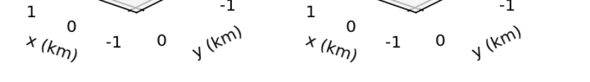
Figure 8: Slices of the $4$-dimensional $50$-step RC set for a spacecraft rendezvous problem. (Left) Initial $v_{x}=0$. (Right) Initial $v_{y}=0$.

Fig. 8 shows the slices of the RC set computed using the ConstrainedZonotope class of pycvxset. We faced numerical issues when performing polytope-based computations of RC sets which may be attributed to the difficulties arising vertex-halfspace enumeration. The computation of the RC set using ConstrainedZonotope took about $30$ seconds.

V-C Admissible deviations from a given robot trajectory

We now demonstrate how pycvxset and ConstrainedZonotope class may be used to compute projections and slices of high-dimensional polytopes.

Consider a robot moving in 2D space with (unperturbed) dynamics along each dimension given by a double integrator system (34). While one can use convex optimization to design minimum-energy, dynamically-feasible, trajectories passing through a collection of waypoints, we consider the problem of characterizing all positions that the robot may deviate to while following the trajectory using pycvxset.

For a horizon $N$, position waypoints $z_{i,\text{pos}}\in\mathbb{R}^{2}$ with $i\in\mathcal{I}\subset\mathbb{N}$, dynamics $(A,B)$, initial state $x_{0}$, and input constraint set $\mathcal{U}\subset\mathbb{R}^{2}$, we define the set of admissible trajectories $\mathcal{D}\subset\mathbb{R}^{4N}$ as follows,

$$\mathcal{D}=\left\{\left[\begin{array}[]{c}x_{1}\\ \vdots\\ x_{N}\end{array}\right]\in\mathbb{R}^{4N}\middle|\begin{array}[]{c}\forall t\in\{0,1,\ldots,N-1\},\\ \exists u_{t}\in\mathcal{U},\ x_{t+1}=Ax_{t}+Bu_{t},\\ \forall i\in\mathcal{I},\ [I_{2},0_{2\times 2}]x_{i}=z_{i,\text{pos}}\\ \end{array}\right\}.$$ (41)

We compute $\mathcal{D}$ in pycvxset via an affine transformation of the open-loop control sequence set $\mathcal{U}^{N}$, where the transformation $(M,v)$ (see Table I) is characterized by $x_{0},A,B,N$. We then slice the transformed set at appropriate dimensions to enforce the position of robot at time $i$ is $z_{i,\text{pos}}$ for each $i\in\mathcal{I}$. In other words, the set $\mathcal{D}$ is a slice of a forward reachable set [3]. While such computations are numerically challenging for polytopes due to the vertex-halfspace enumeration involved for high-dimensional polytopes, these sets are easily characterized using constrained zonotopes.

Figure 9: (Top) Original waypoints, feasible robot trajectory passing through the waypoints, and the admissible deviations at different time steps. While the first few and the penultimate time steps do not admit any deviations, the rest of the time steps (not in $\mathcal{I}$) admit deviations. (Bottom) We generate a new waypoint from the admissible deviation set at time step $t=5$, and alter the robot trajectory to pass through the new waypoint.

Fig. 9 (top) illustrates the set of admissible deviation positions and a dynamically feasible trajectory passing through these waypoints for $N=10$, dynamics with sampling time as $0.5$ seconds, and a set of waypoint position constraints at $\mathcal{I}=\{2,4,6,9\}$. We choose initial state $x_{0}=[0,0,0,0]$, and input constraint set $\mathcal{U}=\{u\in\mathbb{R}^{2}:-1\leq u\leq 1\}$ (in ms^-2). For ease in plotting, we defined separate sets of admissible deviation positions for each time $t\in\{1,3,5,7,8\}$, and restricted the velocity at these deviation positions to be zero. For the given set of waypoints, we found that no such admissible waypoint exists for $t=1$. The set of all such admissible deviation positions over any time step covers an area of about $0.067$ m², which is around $42\%$ of the operating area $[0,0.45]\times[0,0.35]$ (in m).

Fig. 9 (bottom) illustrates an altered trajectory to reach close to $(0.4,0.3)$ at $t=5$.

VI Conclusion

This paper introduces pycvxset, an open-source Python package to manipulate and visualize convex sets in Python. Currently, pycvxset supports polytopic, ellipsoidal, and constrained zonotopic set representations. The packages facilitates the use of set-based methods to analyze and control dynamical systems in Python.

VII Acknowledgements

We are grateful to Stefano Di Cairano and Kieran Parsons for their insightful feedback during the course of the development of this package.

References

- [1] F. Blanchini and S. Miani, Set-theoretic methods in control. Springer, 2008.
- [2] D. Bertsekas and I. Rhodes, “On the minimax reachability of target sets and target tubes,” Automatica, vol. 7, 1971.
- [3] F. Borrelli, A. Bemporad, and M. Morari, Predictive control for linear and hybrid systems. Cambridge Univ. Press, 2017.
- [4] M. Althoff, G. Frehse, and A. Girard, “Set propagation techniques for reachability analysis,” Annual Rev. Ctrl., Rob., & Auto. Syst., vol. 4, no. 1, pp. 369–395, 2021.
- [5] A. Vinod, A. Weiss, and S. Di Cairano, “Abort-safe spacecraft rendezvous under stochastic actuation and navigation uncertainty,” in Proc. Conf. Dec. & Ctrl., 2021, pp. 6620–6625.
- [6] ——, “Projection-free computation of robust controllable sets with constrained zonotopes,” arXiv preprint arXiv:2403.13730, 2024.
- [7] ——, “Inscribing and separating an ellipsoid and a constrained zonotope: Applications in stochastic control and centering,” in Proc. Conf. Dec. & Ctrl., 2024, (accepted).
- [8] J. Scott, D. Raimondo, G. Marseglia, and R. Braatz, “Constrained zonotopes: A new tool for set-based estimation and fault detection,” Automatica, vol. 69, pp. 126–136, 2016.
- [9] V. Raghuraman and J. Koeln, “Set operations and order reductions for constrained zonotopes,” Automatica, 2022.
- [10] L. Yang, H. Zhang, J. Jeannin, and N. Ozay, “Efficient backward reachability using the Minkowski difference of constrained zonotopes,” IEEE Tran. Comp.-Aided Design Integrated. Circ. & Syst., vol. 41, no. 11, pp. 3969–3980, 2022.
- [11] A. Kurzhanskiy and P. Varaiya, “Ellipsoidal toolbox (ET),” in Proc. Conf. Dec. & Ctrl., 2006, http://systemanalysisdpt-cmc-msu.github.io/ellipsoids/.
- [12] “pycddlib,” https://pypi.org/project/pycddlib/.
- [13] “pytope,” https://github.com/heirung/pytope.
- [14] “polytope,” https://tulip-control.github.io/polytope/.
- [15] “pypoman,” https://pypi.org/project/pypoman/.
- [16] M. Althoff, “An introduction to CORA,” in W. App. Verif. Cont. & Hyb. Syst., 2015, pp. 120–151.
- [17] M. Herceg, M. Kvasnica, C. Jones, and M. Morari, “Multi-Parametric Toolbox 3.0,” in Proc. Euro. Ctrl. Conf., 2013.
- [18] J. Koeln, T. J. Bird, J. Siefert, J. Ruths, H. Pangborn, and N. Jain, “zonoLAB: A MATLAB toolbox for set-based control systems analysis using hybrid zonotopes,” arXiv preprint arXiv:2310.15426, 2023.
- [19] S. Boyd and L. Vandenberghe, Convex optimization. Cambridge Univ. Press, 2004.
- [20] J. Gleason, A. Vinod, and M. M. Oishi, “Lagrangian approximations for stochastic reachability of a target tube,” Automatica, vol. 128, 2021.
- [21] A. Vinod, J. Gleason, and M. M. K. Oishi, “SReachTools: A MATLAB Stochastic Reachability Toolbox,” in Proc. Hyb. Syst.: Comput. & Ctrl., Montreal, Canada, 2019, https://sreachtools.github.io.
- [22] T. Lipp and S. Boyd, “Variations and extension of the convex–concave procedure,” Opt. & Engg., vol. 17, pp. 263–287, 2016.
- [23] I. Kolmanovsky and E. G. Gilbert, “Theory and computation of disturbance invariant sets for discrete-time linear systems,” Mathematical problems in engineering, vol. 4, no. 4, 1998.