Filtering coupled Wright–Fisher diffusions

Coupled Wright–Fisher diffusions have been recently introduced to model the temporal evolution of finitely-many allele frequencies at several loci. These are vectors of multidimensional diffusions whose dynamics are weakly coupled among loci through interaction coefficients, which make the reproductive rates for each allele depend on its frequencies at several loci. Here we consider the problem of filtering a coupled Wright–Fisher diffusion with parent-independent mutation, when this is seen as an unobserved signal in a hidden Markov model. We assume individuals are sampled multinomially at discrete times from the underlying population, whose type configuration at the loci is described by the diffusion states, and adapt recently introduced duality methods to derive the filtering and smoothing distributions. These respectively provide the conditional distribution of the diffusion states given past data, and that conditional on the entire dataset, and are key to be able to perform parameter inference on models of this type. We show that for this model these distributions are countable mixtures of tilted products of Dirichlet kernels, and describe their mixing weights and how these can be updated sequentially. The evaluation of the weights involves the transition probabilities of the dual process, which are not available in closed form. We lay out pseudo codes for the implementation of the algorithms, discuss how to handle the unavailable quantities, and briefly illustrate the procedure with synthetic data.

Keywords: Duality; Bayesian inference; Hidden Markov model; Smoothing; Reversibility.

1 Introduction

Wright–Fisher (WF) Markov chains and their diffusion approximations are among the most widely used stochastic models in mathematical biology. See, e.g., Maruyama (1977); Ewens (1979); Ethier and Kurtz (1986); Dawson (1993); Etheridge (2009); Feng (2010). Recently they have also been seen as a temporally evolving parameter which becomes the inferential goal in a Bayesian statistical problem; see Chaleyat-Maurel and Genon-Catalot (2009); Papaspiliopoulos and Ruggiero (2014); Kon Kam King et al. (2021; 2024). See also Papaspiliopoulos et al. (2016); Ascolani et al. (2021; 2023) for nonparametric extensions involving Fleming–Viot and Dawson–Watanabe measure-valued diffusions and Ascolani et al. (2024) for related software.

Coupled Wright–Fisher (c-WF) diffusions extend classical WF diffusions to weakly dependent vectors of WF diffusions. These vectors model the temporal evolution of allelic frequencies in a multi-locus multi-allelic process when pairwise interactions can occur among different loci. Pairwise interactions are expressed in terms of selection coefficients, leading to weak coupling mechanisms as they affect the reproduction rates of the alleles. This class of models was introduced by Aurell et al. (2019) as the scaling limit of a Moran-type population of haploid, asexually reproducing individuals with mutation and inter-locus selection, motivated by the evolution of certain populations of bacteria where the dependence between loci can be effectively encoded by a selection mechanism. Setting the inter-locus selection parameters as null yields as a special case a collection of independent WF diffusions with selection as they appear, e.g., in Barbour et al. (2000). See also Ewens (2004), Chapters 6-7, and Ethier and Nagylaki (1989) for previous contributions related to the multi-locus case. Favero et al. (2021) identified a dual jump process for c-WF diffusions (the notion of duality will be recalled in Section 2.3 below), while García-Pareja et al. (2021) investigated their exact simulation when mutations are parent-independent and the stationary distribution is available. Different and stronger coupling mechanisms, which for example produce interacting diffusions via migration of individuals in underlying structured populations, had been previously studied, among others, in Vaillancourt (1990); Dawson et al. (1995); Dawson and Greven (1999); Greven et al. (2001; 2005). See also Pruenster and Ruggiero (2013) for a Bayesian nonparametric interpretation of a class of interacting Fleming–Viot models through Pólya urn schemes.

In this paper we study the distributional properties of c-WF diffusions with parent-independent mutations in presence of data collected at discrete times from the underlying population. We consider a hidden Markov model statistical framework (Cappé et al., 2005), whereby the c-WF diffusion describes a temporally evolving unobserved signal, which is the primary object of inference, and we assume incomplete observations are collected at a set of discrete time points from an appropriate distribution which reflects the underlying population structure. In particular, since the data collection reveals partial information on the population composition through a non linear link, this inferential problem does not fall into the realm of Kalman-type filtering (Bain and Crisan, 2009; Cappé et al., 2005). Given such data collection framework, we identify the conditional distributions of the diffusion states given past data (signal prediction), given past and present data (filtering) and given the entire dataset, including data collected at later times (marginal smoothing). These distributions constitute the fundamental tools in view of performing parameter inference for a hidden Markov model. The latter, in particular, is often used to improve previous estimates, obtained through filtering, once new data are collected at later times, which typically result in smoother estimates. We obtain these results by adapting a strategy based on duality proposed by Kon Kam King et al. (2024), leveraging on the knowledge of the dual process which was investigated in Favero et al. (2021). The implementation of the above ingredients and recipes is not immediate in that we first have to show that the model at hand satisfies certain requirements, which include showing the model is reversible, then we have to identify the family of likelihoods that allows to perform the envisioned calculations, and finally we have to identify correctly the quantities that appear in the final distributions. Our result provide a description of the recursions that allow to compute the filtering and the smoothing distributions, overcoming the unavailability of the transition function of the c-WF diffusion, which in principle is involved in the evaluation of these distributions.

The paper is organized as follows. In Section 2 we first recall generalities about c-WF diffusions, and then show that, under the assumption of parent-independent mutations, they are reversible with respect to their stationary distribution, which is a product of tilted Dirichlet distributions. We also recall the dual process of these diffusions, which is a multidimensional continuous-time Markov chain. In Section 3 we formulate the inferential problem of interest as a hidden Markov model driven by a c-WF diffusion and, leveraging on the shown reversibility, we derive the filtering and smoothing distributions when the data are assumed to be collected from products of multinomial densities parameterized by the signal at several discrete time points. We show that the marginal distributions of c-WF states are mixtures of products of tilted Dirichlet distributions, and we describe how to update the time-dependent mixture weights based on the previous available conditional distribution. This in turn allows to devise algorithms that, starting from an initial distribution arbitrarily chosen within the same class as the stationary distribution, allow to recursively compute the marginal distributions of the process states, conditional on past data or conditionally on the entire dataset. These algorithms are laid out in Section 4, which also presents a brief illustration of the filtering procedure with synthetic data. We also we discuss implementation issues, particularly concerning numerical methods for dealing with the dual process transitions, which are not available in closed form, and some other unavailable normalizing constants, through Monte Carlo procedures.

2 Coupled Wright–Fisher diffusions

2.1 Generalities

Define the space

$$\Delta=\times_{l=1}^{L}\Delta_{K_{l}},\quad\Delta_{K_{l}}=\bigg{\{}\mathbf{x}\in[0,1]^{K_{l}}:\sum_{i=1}^{K_{l}}x_{i}^{(l)}=1\bigg{\}},$$

where $L\geq 1$ denotes the number of loci, $K_{1},\ldots,K_{L}$ are positive integers representing the amount of alleles at each locus and $K=\sum_{l=1}^{L}K_{l}$ is the total number of alleles among all loci. Following Favero et al. (2021), a coupled Wright–Fisher (c-WF) diffusion is the $\Delta$-valued strong solution of

$$\mathrm{d}\mathbf{X}(t)=\mu(\mathbf{X}(t))\mathrm{d}t+D(\mathbf{X}(t))\nabla V(\mathbf{X}(t))\mathrm{d}t+D^{1/2}(\mathbf{X}(t))\mathrm{d}\textbf{W}(t),$$ (1)

where $\mathbf{W}=\left(\mathbf{W}^{(1)},\ldots,\mathbf{W}^{(L)}\right)^{T}$ is a multi-dimensional Brownian motion, each $\mathbf{W}^{(l)}$ having the same dimension as $\mathbf{X}^{(l)}$. Here $\mathbf{X}(t)$ is a concatenation of the $L$ vectors

$$\mathbf{X}^{(l)}(t)=\Big{(}X_{1}^{(l)}(t),\ldots,X_{K_{l}}^{(l)}(t)\Big{)}^{T},$$

where $X_{i}^{(l)}(t)$ is the relative frequency of the $i$-th type among those at locus $l$ at time $t$. In particular, drift and diffusion coefficients are defined as

$$\mu(\mathbf{x})=\left(\begin{array}[]{c}\mu^{(1)}\left(\mathbf{x}^{(1)}\right)\\ \vdots\\ \mu^{(L)}\left(\mathbf{x}^{(L)}\right)\end{array}\right),\quad\quad D(\mathbf{x})=\left(\begin{array}[]{ccc}D^{(1)}\left(\mathbf{x}^{(1)}\right)&\\ &\ddots&\\ &&D^{(L)}\left(\mathbf{x}^{(L)}\right)\end{array}\right),$$

with $\mu^{(l)}:\mathbb{R}^{K_{l}}\rightarrow\mathbb{R}^{K_{l}}$ and $D^{(l)}:\mathbb{R}^{K_{l}}\rightarrow\mathbb{R}^{K_{l}\times K_{l}}$, for all $l=1,\ldots,L$. The drift vector $\mu$ drives mutations, which in our case are assumed to be parent-independent and independent of other loci, with the infinitesimal rate of mutation from type $i$ to $j$ at locus $l$ equal to $\alpha_{ij}^{(l)}=\alpha_{j}^{(l)}/2$. The drift component for type $i$ type at locus $l$ thus is

$$\mu_{i}^{(l)}(\mathbf{x}^{(l)})=\sum_{j=1}^{K_{l}}(\alpha_{ji}^{(l)}x_{j}^{(l)}-\alpha_{ij}^{(l)}x_{i}^{(l)})=\dfrac{1}{2}(\alpha_{i}^{(l)}-|\boldsymbol{\alpha}^{(l)}|x_{i}^{(l)}),$$

where $|\boldsymbol{\alpha}^{(l)}|=\sum_{i=1}^{K_{l}}\alpha_{i}^{(l)}$ and $\boldsymbol{\alpha}^{(l)}=(\alpha_{1}^{(l)},\ldots,\alpha_{K_{l}}^{(l)})$. The diffusion terms are of the usual form for WF-type models, namely

$$d_{ij}^{(l)}(\mathbf{x}^{(l)})=x_{i}^{(l)}(\delta_{ij}-x_{j}^{(l)}),\quad\quad\delta_{ij}=\begin{cases}1,\quad\text{if }i=j\\ 0,\quad\text{if }i\neq j,\end{cases}$$

The coupling of the $L$ WF diffusions involved in the model is controlled by the selection drift term $D\ \nabla V_{\boldsymbol{\sigma},\mathbf{J}}$, where $V_{\boldsymbol{\sigma},\mathbf{J}}:[0,1]^{K}\rightarrow\mathbb{R}$ is defined as

$$V_{\boldsymbol{\sigma},\mathbf{J}}(\mathbf{x})=\mathbf{x}^{T}\boldsymbol{\sigma}+\frac{1}{2}{\mathbf{x}}^{T}\mathbf{J}\mathbf{x}.$$ (2)

Here $\boldsymbol{\sigma}\in\mathbb{R}_{+}^{K}$ is the vector of single-locus selection parameters, whereas $\mathbf{J}\in\mathbb{R}_{+}^{K\times K}$ is a symmetric block matrix containing only two-locus selection parameters, that is $\mathbf{J}^{(lr)}=\left(\mathbf{J}^{(rl)}\right)^{T}\in\mathbb{R}^{K_{l}\times K_{r}}$ for all $l,r=1,\ldots,L$, with null sub-matrices $\mathbf{J}^{(ll)}=\textbf{O}\in\mathbb{R}^{K_{l}\times K_{l}}$ on the diagonal, where O denotes a matrix of zeros. The interaction term $\eqref{V}$ is also known as fitness potential, see Aurell et al. (2019) for further discussion. Thus (2) includes selection coefficients that apply both within a single locus, as in classical WF diffusions, and among different loci. In the latter case, these generate a weak interaction among the frequencies at these loci by affecting the respective reproduction rates. Therefore (1) is a system of $L$ equations, each reflecting the dynamics of the frequencies at a single locus, coupled through the drift term $D\ \nabla V_{\boldsymbol{\sigma},\mathbf{J}}$. When $\nabla V_{\boldsymbol{\sigma},\mathbf{J}}=0$, there is no interaction among loci and (1) reduces to a system of $L$ independent WF diffusions each solving

$$\mathrm{d}\mathbf{X}^{(l)}(t)=\mu^{(l)}(\mathbf{X}^{(l)}(t))\mathrm{d}t+D^{(l)1/2}(\mathbf{X}^{(l)}(t))\mathrm{d}\textbf{W}^{(l)}(t).$$

Alternatively, we can define the c-WF diffusion through its infinitesimal generator. By definition of $V$, we have $\nabla V_{\boldsymbol{\sigma},\mathbf{J}}(\mathbf{x})=\boldsymbol{\sigma}+\mathbf{J}\mathbf{x}$, which implies that the components $g(\mathbf{x}):=D(\mathbf{x})\nabla V_{\boldsymbol{\sigma},\mathbf{J}}(\mathbf{x})$ are of the form

$$g_{i}^{(l)}(\mathbf{x})=\sum_{k=1}^{K_{l}}d_{ik}^{(l)}(\mathbf{x}^{(l)})\tilde{\sigma}_{k}^{(l)}(\mathbf{x})\quad\text{ with }\quad\tilde{\sigma}_{k}^{(l)}(\mathbf{x})=\sigma_{k}^{(l)}+\sum_{\begin{subarray}{c}r=1\\ r\neq l\end{subarray}}^{L}\sum_{h=1}^{K_{r}}J_{kh}^{(lr)}x_{h}^{(r)}.$$

Then the infinitesimal generator $\mathcal{A}$ of the c-WF diffusion, with domain $D(\mathcal{A})=C^{2}(\Delta)$, is

$$\mathcal{A}=\sum_{l=1}^{L}\sum_{i=1}^{K_{l}}\left(\mu_{i}^{(l)}(\mathbf{x}^{(l)})+g_{i}^{(l)}(\mathbf{x})\right)\frac{\partial}{\partial x_{i}^{(l)}}+\frac{1}{2}\sum_{l=1}^{L}\sum_{i,j=1}^{K_{l}}d_{ij}^{(l)}(\mathbf{x}^{(l)})\frac{\partial^{2}}{\partial x_{i}^{(l)}\partial x_{j}^{(l)}}.$$ (3)

When $\mathbf{J}$ vanishes, (3) reduces to the sum of $L$ generators

$$\mathcal{A}_{0}^{(l)}=\sum_{i=1}^{K}\left[\dfrac{1}{2}\left(\alpha_{i}-|\boldsymbol{\alpha}|x_{i}\right)+\sum_{k=1}^{K}\sigma_{k}^{(l)}x_{i}(\delta_{ik}-x_{k})\right]\dfrac{\partial}{\partial x_{i}}+\dfrac{1}{2}\sum_{i,j=1}^{K}x_{i}\left(\delta_{ij}-x_{j}\right)\dfrac{\partial^{2}}{\partial x_{i}\partial x_{j}}$$ (4)

which describe a collection of $L$ independent WF diffusions with selection.

2.2 Reversibility

It is well known that the Dirichlet distribution is the invariant measure of the single-locus WF diffusion with parent-independent mutation, cf. Ethier and Griffiths (1993), and a tilted Dirichlet distribution is the invariant measure in presence of single-locus selection, cf. Barbour et al. (2000). Denote by

$$\pi_{\boldsymbol{\alpha}}(\mathrm{d}\mathbf{x})=\mathbf{x}^{\boldsymbol{\alpha}-1}\mathrm{d}\mathbf{x}=\prod_{l=1}^{L}\left(\mathbf{x}^{(l)}\right)^{\boldsymbol{\alpha}^{(l)}-1}\mathrm{d}\mathbf{x}^{(l)}=\prod_{l=1}^{L}\prod_{i=1}^{K_{l}}\big{(}x_{i}^{(l)}\big{)}^{\alpha_{i}^{(l)}-1}\mathrm{d}x_{i}^{(l)}$$ (5)

a product of unnormalised Dirichlet densities, where $\boldsymbol{\alpha}=(\boldsymbol{\alpha}^{(1)},\ldots,\boldsymbol{\alpha}^{(L)})$ and $\boldsymbol{\alpha}^{(l)}=(\alpha_{1}^{(l)},\ldots,\alpha_{K_{l}}^{(l)})$ as above. When inter-locus selection is described by (2), it was shown in Aurell et al. (2019) that the c-WF process has invariant distribution

$$p_{\boldsymbol{\alpha},\boldsymbol{\sigma},\mathbf{J}}(\mathrm{d}\mathbf{x})=Z^{-1}\pi_{\boldsymbol{\alpha}}(\mathrm{d}\mathbf{x})e^{2V_{\boldsymbol{\sigma},\mathbf{J}}(\mathbf{x})},$$ (6)

where $Z$ denotes the normalising constant. When $\mathbf{J}$ vanishes, we recover a product of stationary distribution of $L$ independent WF process as in (4), namely in each locus $l\in L$,

$$p_{\boldsymbol{\alpha},\boldsymbol{\sigma}}(\mathrm{d}\mathbf{x})\propto\mathbf{x}^{\boldsymbol{\alpha}-1}e^{2\mathbf{x}^{T}\boldsymbol{\sigma}}\mathrm{d}\mathbf{x}=\prod_{i=1}^{K}x_{i}^{\alpha_{i}-1}e^{2x_{i}\sigma_{i}}\mathrm{d}x_{i},$$

similar to Barbour et al. (2000).

Our first result extends the above stationarity and shows that (6) is also the reversible measure for (3).

Proposition 2.1.

The coupled Wright–Fisher diffusion with generator (3) is reversible with respect to (6).

Proof.

We leverage on a Theorem 4.6 of Fukushima and Stroock (1986), where some symmetry-preserving transformations of measure and infinitesimal generator are provided. Specifically, by expanding the interaction function $V_{\boldsymbol{\sigma},\mathbf{J}}\in C^{2}(\Delta)$,

$$V_{\boldsymbol{\sigma},\mathbf{J}}(\mathbf{x})=\mathbf{x}^{T}\boldsymbol{\sigma}+\frac{1}{2}\mathbf{x}^{T}\mathbf{J}\mathbf{x}=\sum_{l=1}^{L}\sum_{i=1}^{K_{l}}\bigg{[}x^{(l)}_{i}\sigma^{(l)}_{i}+\frac{1}{2}x^{(l)}_{i}\sum_{\begin{subarray}{c}r=1\\ r\neq l\end{subarray}}^{L}\sum_{j=1}^{K_{r}}J^{(lr)}_{ij}x^{(r)}_{j}\bigg{]},$$

it follows that (3) can be written as

$$\mathcal{A}=\mathcal{A}_{0}+\sum_{l=1}^{L}\sum_{i=1}^{K_{l}}\bigg{[}\sum_{k=1}^{K_{l}}a^{(l)}_{ik}\left(\mathbf{x}\right)\frac{\partial}{\partial x^{(l)}_{k}}V_{\boldsymbol{\sigma},\mathbf{J}}(\mathbf{x})\bigg{]}\frac{\partial}{\partial x^{(l)}_{i}},$$ (7)

where

$$a^{(l)}_{ik}=x_{i}(\delta_{ik}-x_{k}),$$

and

$$\frac{\partial}{\partial x^{(l)}_{k}}V_{\boldsymbol{\sigma},\mathbf{J}}(\mathbf{x})=\sigma^{(l)}_{k}+\frac{1}{2}\sum_{\begin{subarray}{c}r=1\\ r\neq l\end{subarray}}^{L}\sum_{j=1}^{K_{r}}J^{(lr)}_{kj}x^{(r)}_{j},$$

and $\mathcal{A}_{0}$ is the infinitesimal generator of the multi-locus WF diffusion without selection. The latter is known to be symmetric with respect to (5) (cf. Ethier and Kurtz, 1981, Lemma 4.1), in the sense that $\int f(\mathcal{A}_{0}g)\mathrm{d}\pi_{\alpha}=\int g(\mathcal{A}_{0}f)\mathrm{d}\pi_{\alpha}$ for all $f,g\in D(\mathcal{A}_{0})$. Then, by virtue of (7), it follows that $\mathcal{A}$ is symmetric with respect to (6). ∎

The reversibility established above will be needed in Section 3 to study filtering and smoothing for c-WF diffusions.

2.3 Duality

Given two Markov processes $\{X(t):t\geq 0\}$ and $\{M(t):t\geq 0\}$ on $\mathcal{S}$ and $\mathcal{S}^{\prime}$ respectively, we say $X(t)$ is dual to $M(t)$ with respect to a bounded measurable function $h:\mathcal{S}\times\mathcal{S}^{\prime}\rightarrow\mathbb{R}$ if

$$\mathbb{E}\left[h(X(t),m)\mid X(0)=x\right]={\mathbb{E}}\left[h(x,M(t))\mid M(0)=m\right]\qquad\forall x\in\mathcal{S},m\in\mathcal{S}^{\prime},t>0.$$ (8)

See Ethier and Kurtz (1986); Jansen and Kurt (2014) for reviews, details and applications. Favero et al. (2021) identified a multivariate jump process on $\mathbb{N}^{K}$, which we will define below, as dual to a c-WF diffusion with respect to function

$$h(\mathbf{x},\mathbf{m})=\frac{1}{k(\mathbf{m})}\mathbf{x}^{\mathbf{m}}=\frac{1}{k(\mathbf{m})}\prod_{l=1}^{L}\prod_{i=1}^{K_{l}}\left(x_{i}^{(l)}\right)^{m_{i}^{(l)}},$$ (9)

where, for $\tilde{\mathbf{X}}\sim p_{\boldsymbol{\alpha},\boldsymbol{\sigma},\mathbf{J}}(\mathrm{d}\mathbf{x})$,

$$k(\mathbf{m})=\mathbb{E}\bigg{[}\prod_{l=1}^{L}\prod_{i=1}^{K_{l}}\big{(}\tilde{X}_{i}^{(l)}\big{)}^{m_{i}^{(l)}}\bigg{]}.$$

Notice also that (9) is of the same form as the duality function for the single-locus case in Etheridge and Griffiths (2009); Papaspiliopoulos and Ruggiero (2014); Griffiths et al. (2019), since this model is labelled, as opposed, e.g., to Griffiths et al. (2024).

Let $\mathbf{e}_{i}^{(l)}$ be the standard unit vector in $\mathbb{R}^{K}$ in the $i$-th direction on the $l$-th locus. In the special case with parent-independent mutations, the dual process is a pure-jump Markov process $\mathbf{M}:=\{\mathbf{M}(t),t\geq 0\}$, with $\mathbf{M}(t)\in\mathbb{N}^{K}$, which jumps from $\mathbf{m}\in\mathbb{N}^{K}\backslash\left\{\textbf{0}\right\}$ to

• $\mathbf{m}-\mathbf{e}_{i}^{(l)}$ (coalescence) for $i=1,\ldots K_{l},\ l=1,\ldots,L$, s.t. $m_{i}^{(l)}\geq 2$, at rate

  $$q\left(\mathbf{m},\mathbf{m}-\mathbf{e}_{i}^{(l)}\right)=\dfrac{m_{i}^{(l)}(m_{i}^{(l)}-1)}{2}\dfrac{k(\mathbf{m}-\mathbf{e}_{i}^{(l)})}{k(\mathbf{m})};$$

• $\mathbf{m}-\mathbf{e}_{i}^{(l)}+\mathbf{e}_{j}^{(l)}$ (mutation) for $i,j=1,\ldots K_{l},\ l=1,\ldots,L$, s.t. $i\neq j,m_{i}^{(l)}\geq 1$, at rate

  $$q\left(\mathbf{m},\mathbf{m}-\mathbf{e}_{i}^{(l)}+\mathbf{e}_{j}^{(l)}\right)=m_{i}^{(l)}\dfrac{\alpha_{i}^{(l)}}{2}\dfrac{k(\mathbf{m}-\mathbf{e}_{i}^{(l)}+\mathbf{e}_{j}^{(l)})}{k(\mathbf{m})};$$

• $\mathbf{m}+\mathbf{e}_{j}^{(l)}$ (branching) for $j=1,\ldots K_{l},\ l=1,\ldots,L$, at rate

  $$q\left(\mathbf{m},\mathbf{m}+\mathbf{e}_{j}^{(l)}\right)=\Bigl{(}|\mathbf{m}^{(l)}|\sum_{\begin{subarray}{c}k=1\\ k\neq j\end{subarray}}^{K_{l}}\sigma_{k}^{(l)}+\sum_{\begin{subarray}{c}r=1\\ r\neq l\end{subarray}}^{L}\sum_{i=1}^{K_{r}}m_{i}^{(r)}J_{ji}^{(lr)}\Bigr{)}\dfrac{k(\mathbf{m}+\mathbf{e}_{j}^{(l)})}{k(\mathbf{m})};$$ (10)

• $\mathbf{m}+\mathbf{e}_{j}^{(l)}+\mathbf{e}_{h}^{(r)}$ (double branching) for $j=1\ldots K_{l},\ h=1\ldots,K_{r},\ l,r=1,\ldots,L,\ r>l$, at rate

  $$q\left(\mathbf{m},\mathbf{m}+\mathbf{e}_{j}^{(l)}+\mathbf{e}_{h}^{(r)}\right)=\Bigl{[}\left(|\mathbf{m}^{(l)}|+|\mathbf{m}^{(r)}|\right)\sum_{\begin{subarray}{c}k=1\\ k\neq j\end{subarray}}^{K_{l}}\sum_{\begin{subarray}{c}n=1\\ n\neq h\end{subarray}}^{K_{r}}J_{kn}^{(lr)}\Bigr{]}\dfrac{k(\mathbf{m}+\mathbf{e}_{j}^{(l)}+\mathbf{e}_{h}^{(r)})}{k(\mathbf{m})},$$

where $|\mathbf{m}^{(l)}|=\sum_{i=1}^{K_{l}}m_{i}^{(l)}$. See Favero et al. (2021) for further details and interpretation.

3 Filtering coupled Wright–Fisher diffusions

We are going to cast c-WF diffusions in a hidden Markov model statistical framework, whose general structure will be recalled shortly, and derive, under certain assumptions on the data collection, the conditional distributions of the diffusion states under different types of conditioning: on past data, leading to the signal predictive distribution; on past and present data, leading to the filtering distribution; and on the entire dataset, that is including observation that become available at a later time, leading to marginal smoothing distributions.

A hidden Markov model (HMM) is defined by a two-component process $\left\{\left(X_{n},Y_{n}\right):n\geq 0\right\}$, where $X_{n}$ is an unobserved Markov chain, often called latent signal, while $Y_{n}$ denotes the observation (or the vector of observations) collected at step $n$. Such a pair is a HMM if the distribution of $Y_{n}$ only depends on the value of $X_{n}$, plus possibly additional global parameters, making $Y_{n}$ conditionally independent of $X_{k},Y_{k},k\neq n$, given $X_{n}$. See Cappé et al. (2005) for a general treatment of HMMs.

Here we consider the signal to be the discrete-time skeleton of a c-WF diffusion, that is, if $\mathbf{X}$ has generator (3), we let $X_{n}:=\mathbf{X}(t_{n})$ for $0=t_{0}<t_{1}<\cdots<T$. Note that the intervals between data collection times need not be equal. We assume the following specification for the HMM:

$$\mathbf{X}\sim \,\text{c-WF}_{\boldsymbol{\alpha},\boldsymbol{\sigma},\mathbf{J}},\quad\mathbf{X}(0)\sim p_{\boldsymbol{\alpha},\boldsymbol{\sigma},\mathbf{J}},$$ (11)

$$\mathbf{Y}(t_{n})|\mathbf{X}(t_{n})=\mathbf{x} \,\sim\text{MN}_{L}(\mathbf{N}_{n},\mathbf{x})$$

where $\mathbf{X}\sim\text{c-WF}_{\boldsymbol{\alpha},\boldsymbol{\sigma},\mathbf{J}}$ denotes that $\mathbf{X}$ is a c-WF diffusion with operator (3), $p_{\boldsymbol{\alpha},\boldsymbol{\sigma},\mathbf{J}}$ is the initial distribution chosen as in (6), and

$$\text{MN}_{L}(\mathbf{N}_{n},\mathbf{x})=\prod_{l=1}^{L}\text{MN}(N_{n}^{(l)},\mathbf{x}^{(l)})$$

where $\text{MN}(N_{n}^{(l)},\mathbf{x}^{(l)})$ denotes a Multinomial pdf with size $N_{n}^{(l)}$ and categorical probabilities $\mathbf{x}^{(l)}=(\mathbf{x}^{(l)}_{1},\ldots,\mathbf{x}^{(l)}_{K})$. Here the values in $\mathbf{N}_{n}=(N_{n}^{(1)},\ldots,N_{n}^{(L)})$ are assumed to be given for each observation time $t_{n}$.

Note now that (6) and (9) imply

$$\mathbf{x}^{\mathbf{n}}p_{\boldsymbol{\alpha},\boldsymbol{\sigma},\mathbf{J}}(\mathrm{d}\mathbf{x})\propto h(\mathbf{x},\mathbf{n})p_{\boldsymbol{\alpha},\boldsymbol{\sigma},\mathbf{J}}(\mathrm{d}\mathbf{x})=p_{\boldsymbol{\alpha}+\mathbf{n},\boldsymbol{\sigma},\mathbf{J}}(\mathrm{d}\mathbf{x}),$$ (12)

for all $\mathbf{x}\in\Delta$ and $\mathbf{n}\in\mathbb{N}^{K}\setminus\left\{0\right\}$, where $p_{\boldsymbol{\alpha}+\mathbf{n},\boldsymbol{\sigma},\mathbf{J}}$ defined as in (6) with $\boldsymbol{\alpha}$ replaced by $\boldsymbol{\alpha}+\mathbf{n}$ where $\mathbf{n}=(\mathbf{n}^{(1)},\ldots,\mathbf{n}^{(L)})\in\mathbb{N}^{K}\setminus\left\{0\right\}$ and $\mathbf{n}^{(l)}=(n_{1}^{(l)},\ldots,n_{K_{l}}^{(l)})\in\mathbb{N}^{K_{l}}\setminus\left\{0\right\}$. Then, under (11), the distribution of $\mathbf{X}(t_{0})|\mathbf{Y}(t_{0})$ is $p_{\boldsymbol{\alpha}+\mathbf{n},\boldsymbol{\sigma},\mathbf{J}}(\mathrm{d}\mathbf{x})$ with $\mathbf{n}$ being the vector of multiplicities observed in $\mathbf{Y}(t_{0})$. In general we are interested in the signal predictive distribution, i.e., the law of $\mathbf{X}(t_{n+1})|\mathbf{Y}(t_{0}),\ldots,\mathbf{Y}(t_{n})$, and in the filtering distribution, i.e., the law of $\mathbf{X}(t_{n+1})|\mathbf{Y}(t_{0}),\ldots,\mathbf{Y}(t_{n+1})$. These are no longer single kernels as in (12), but can be computed recursively as described by the next result.

Proposition 3.1.

Let $(\mathbf{X}(t_{n}),\mathbf{Y}(t_{n}))_{n\geq 0}$ be as in (11), and let

$$\mathbf{X}(t_{n})|\mathbf{Y}(t_{0}),\ldots,\mathbf{Y}(t_{n})\sim\sum_{\mathbf{m}>\mathbf{0}}\hat{c}_{n}(\mathbf{m})p_{\boldsymbol{\alpha}+\mathbf{m},\boldsymbol{\sigma},\mathbf{J}}(\mathrm{d}\mathbf{x}),$$ (13)

where $\sum_{\mathbf{m}>\mathbf{0}}\hat{c}_{n}(\mathbf{m})=1$. Then

$$\mathbf{X}(t_{n+1})|\mathbf{Y}(t_{0}),\ldots,\mathbf{Y}(t_{n})\sim\sum_{\mathbf{n}>\mathbf{0}}c_{n+1}(\mathbf{n})p_{\boldsymbol{\alpha}+\mathbf{n},\boldsymbol{\sigma},\mathbf{J}},$$ (14)

where $c_{n+1}(\mathbf{n})\propto\sum_{\mathbf{m}>\mathbf{0}}\hat{c}_{n}(\mathbf{m})p_{\mathbf{m},\mathbf{n}}(t_{n+1}-t_{n})$ and $p_{\mathbf{m},\mathbf{n}}(t)$ are the transition probabilities of M as in Section 2.3. Furthermore, let $\mathbf{Y}(t_{n+1})$ be the data collected at time $t_{n+1}$, with $\mathbf{y}\in\mathbb{N}^{K}\setminus\left\{0\right\}$ describing the observed multiplicities of types, and let $\text{MN}_{L}(\mathbf{y};\mathbf{N}_{n+1},\mathbf{x})$ be as in (11), evaluated at $\mathbf{y}$. Then

$$\mathbf{X}(t_{n+1})|\mathbf{Y}(t_{0}),\ldots,\mathbf{Y}(t_{n+1})\sim\sum_{\mathbf{n}>\mathbf{0}}\hat{c}_{n+1}(\mathbf{n})p_{\boldsymbol{\alpha}+\mathbf{n}+\mathbf{y},\boldsymbol{\sigma},\mathbf{J}},$$

where $\hat{c}_{n+1}(\mathbf{n})\propto c_{n+1}(\mathbf{n})d_{n+1}(\mathbf{m},\mathbf{y})$ and $d_{n+1}(\mathbf{m},\mathbf{y}):=\int_{\Delta}\mathrm{MN}_{L}(\mathbf{y};\mathbf{N}_{n+1},\mathbf{x})p_{\boldsymbol{\alpha}+\mathbf{m},\boldsymbol{\sigma},\mathbf{J}}(\mathrm{d}\mathbf{x})$, with $\mathbf{N}_{n+1}$ the vector of sample sizes collected at time $t_{n+1}$.

Proof.

By virtue of Proposition 2.1, the c-WF diffusion is reversible with respect to (6). Furthermore, the duality identity (8) holds with respect to functions in (9). These yield conditions analogous to Assumptions 1 and 3 in Proposition 2.1 in Kon Kam King et al. (2024), whose implications are spelled out in the rest of the proof. In particular, from these it follows that we can exchange the expectation with respect to the law of $\mathbf{X}(t)$ with the expectation with respect to the law of $\mathbf{M}(t)$, and determine the signal predictive distribution for $\mathbf{X}(t_{n+1})|\mathbf{Y}(t_{0}),\ldots,\mathbf{Y}(t_{n})$ using the dual process transition probabilities, giving rise to a countable mixture of distributions $p_{\boldsymbol{\alpha}+\mathbf{n},\boldsymbol{\sigma},\mathbf{J}}$ with mixture weights $c_{n+1}(\mathbf{n})\propto\sum_{\mathbf{m}>\mathbf{0}}\hat{c}_{n}(\mathbf{m})p_{\mathbf{m},\mathbf{n}}(t_{n+1}-t_{n})$. Indeed, by denoting with $P_{t}(\mathbf{x},\mathrm{d}\mathbf{x}^{\prime})$ the transition semigroup of the c-WF (where the notation $(\mathbf{x},\mathbf{x}^{\prime})$ is equivalent to $(\mathbf{x}^{\prime}|\mathbf{x})$), we see that the law of $\mathbf{X}(t_{n+1})|\mathbf{Y}(t_{0}),\ldots,\mathbf{Y}(t_{n})$ equals

$$\int_{\Delta} \left[\sum_{\mathbf{m}>\mathbf{0}}\hat{c}_{n}(\mathbf{m})p_{\boldsymbol{\alpha}+\mathbf{m},\boldsymbol{\sigma},\mathbf{J}}(\mathrm{d}\mathbf{x})\right]P_{t_{n+1}-t_{n}}\left(\mathbf{x},\mathrm{d}\mathbf{x}^{\prime}\right)$$ (15)

$$=\sum_{\mathbf{m}>\mathbf{0}}\hat{c}_{n}(\mathbf{m})\int_{\Delta}h(\mathbf{x},\mathbf{m})p_{\boldsymbol{\alpha},\boldsymbol{\sigma},\mathbf{J}}(\mathrm{d}\mathbf{x})P_{t_{n+1}-t_{n}}\left(\mathbf{x},\mathrm{d}\mathbf{x}^{\prime}\right).$$ (16)

Proposition 2.1 now implies the detailed balance condition, which here reads

$$p_{\boldsymbol{\alpha},\boldsymbol{\sigma},\mathbf{J}}(\mathrm{d}\mathbf{x})P_{t_{n+1}-t_{n}}(\mathbf{x},\mathrm{d}\mathbf{x}^{\prime})=p_{\boldsymbol{\alpha},\boldsymbol{\sigma},\mathbf{J}}(\mathrm{d}\mathbf{x}^{\prime})P_{t_{n+1}-t_{n}}(\mathbf{x}^{\prime},\mathrm{d}\mathbf{x}),$$

from which the expression in the preceding display is equal to

$$\sum_{\mathbf{m}>\mathbf{0}} \hat{c}_{n}(\mathbf{m})\int_{\Delta}h(\mathbf{x},\mathbf{m})p_{\boldsymbol{\alpha},\boldsymbol{\sigma},\mathbf{J}}\left(\mathrm{d}\mathbf{x}^{\prime}\right)P_{t_{n+1}-t_{n}}\left(\mathbf{x}^{\prime},\mathrm{d}\mathbf{x}\right)$$

$$=\sum_{\mathbf{m}>\mathbf{0}}\hat{c}_{n}(\mathbf{m})p_{\boldsymbol{\alpha},\boldsymbol{\sigma},\mathbf{J}}\left(\mathrm{d}\mathbf{x}^{\prime}\right)\int_{\Delta}h(\mathbf{x},\mathbf{m})P_{t_{n+1}-t_{n}}\left(\mathbf{x}^{\prime},\mathrm{d}\mathbf{x}\right)$$

$$=\sum_{\mathbf{m}>\mathbf{0}}\hat{c}_{n}(\mathbf{m})p_{\boldsymbol{\alpha},\boldsymbol{\sigma},\mathbf{J}}\left(\mathrm{d}\mathbf{x}^{\prime}\right)\mathbb{E}\left[h(\mathbf{X}(t_{n+1}),\mathbf{m})\mid\mathbf{X}(t_{n})=\mathbf{x}^{\prime}\right].$$

Then, from (8) with (9), the previous equals

$$\sum_{\mathbf{m}>\mathbf{0}} \hat{c}_{n}(\mathbf{m})p_{\boldsymbol{\alpha},\boldsymbol{\sigma},\mathbf{J}}\left(\mathrm{d}\mathbf{x}^{\prime}\right)\mathbb{E}\left[h(\mathbf{x}^{\prime},\mathbf{M}(t_{n+1}))\mid\mathbf{M}(t_{n})=\mathbf{m}\right].$$

Writing the expectation as an expansion based on the dual transition probabilities, and rearranging the terms, leads now to

$$\sum_{\mathbf{m}>\mathbf{0}} \hat{c}_{n}(\mathbf{m})p_{\boldsymbol{\alpha},\boldsymbol{\sigma},\mathbf{J}}\left(\mathrm{d}\mathbf{x}^{\prime}\right)\left[\sum_{\mathbf{n}>\mathbf{0}}p_{\mathbf{m},\mathbf{n}}(t_{n+1}-t_{n})h(\mathbf{x}^{\prime},\mathbf{n})\right]$$

$$=\sum_{\mathbf{m}>\mathbf{0}}\sum_{\mathbf{n}>\mathbf{0}}\hat{c}_{n}(\mathbf{m})p_{\mathbf{m},\mathbf{n}}(t_{n+1}-t_{n})h(\mathbf{x}^{\prime},\mathbf{n})p_{\boldsymbol{\alpha},\boldsymbol{\sigma},\mathbf{J}}\left(\mathrm{d}\mathbf{x}^{\prime}\right)$$

$$=\sum_{\mathbf{m}>\mathbf{0}}\sum_{\mathbf{n}>\mathbf{0}}\hat{c}_{n}(\mathbf{m})p_{\mathbf{m},\mathbf{n}}(t_{n+1}-t_{n})p_{\boldsymbol{\alpha}+\mathbf{n},\boldsymbol{\sigma},\mathbf{J}}\left(\mathrm{d}\mathbf{x}^{\prime}\right)$$

$$=\sum_{\mathbf{n}>\mathbf{0}}\sum_{\mathbf{m}>\mathbf{0}}\hat{c}_{n}(\mathbf{m})p_{\mathbf{m},\mathbf{n}}(t_{n+1}-t_{n})p_{\boldsymbol{\alpha}+\mathbf{n},\boldsymbol{\sigma},\mathbf{J}}\left(\mathrm{d}\mathbf{x}^{\prime}\right)$$

$$=\sum_{\mathbf{n}>\mathbf{0}}c_{n+1}(\mathbf{n})p_{\boldsymbol{\alpha}+\mathbf{n},\boldsymbol{\sigma},\mathbf{J}}(\mathrm{d}\mathbf{x}^{\prime}),$$

with $c_{n+1}(\mathbf{n})\propto\sum_{\mathbf{m}>\mathbf{0}}\hat{c}_{n}(\mathbf{m})p_{\mathbf{m},\mathbf{n}}(t_{n+1}-t_{n})$, where we have also used (12).

Clearly, (6) also implies $\mathbf{x}^{\mathbf{y}}p_{\boldsymbol{\alpha}+\mathbf{n},\boldsymbol{\sigma},\mathbf{J}}(\mathrm{d}\mathbf{x})\propto p_{\boldsymbol{\alpha}+\mathbf{n}+\mathbf{y},\boldsymbol{\sigma},\mathbf{J}}(\mathrm{d}\mathbf{x})$. Furthermore, notice that the posterior distribution of a mixture is a mixture of posteriors whose weights are also conditioned on the observations, namely

$$Z\sim\sum_{i}q(i)p_{i}(z)\quad\Rightarrow\quad Z|Y=y\sim\sum_{i}\frac{q(i)p(y|i)}{\sum_{j}q(j)p(y|j)}p_{i}(z|y)$$

given the first is the same as $Z|i\sim p_{i}$ with probability $q(i)$, hence $Z|i,y\sim p_{i}(z|y)$ with probability $q(i|y)$, which is proportional to $q(i)p(y|i)$ by Bayes’s theorem. Hence, we conclude that the filtering distribution for $\mathbf{X}(t_{n+1})|\mathbf{Y}(t_{0}),\ldots,\mathbf{Y}(t_{n+1})$ is a countable mixture of distributions $p_{\boldsymbol{\alpha}+\mathbf{n}+\mathbf{y},\boldsymbol{\sigma},\mathbf{J}}$ with mixture weights $\hat{c}_{n+1}(\mathbf{n})\propto c_{n+1}(\mathbf{n})d_{n}(\mathbf{m},\mathbf{y})$ as given in the statement.

∎

Hence, under (11), the filtering and signal predictive distributions are all identified as countable mixtures of kernels in the same family as (6). These findings fall in the family of filtering distributions described in Chaleyat-Maurel and Genon-Catalot (2006) (cf. eq.(2)), which evolve within the set of countable mixtures of specified parametric kernels. Note however that in the present setting the specific form of the semigroup of the c-WF is unknown, and therefore the sufficient conditions there specified cannot be checked. The same conclusions can nonetheless be drawn here using a duality-based approach.

The mixture weights in Proposition 3.1 depend on the dual process transitional probabilities. We can therefore associate each mixture component to a node of $L$ coupled $K_{l}$-dimensional directed graphs, as illustrated in Figure 1. With $L=2$ loci and $K_{1}=K_{2}=2$ types at each locus, the $4$-dimensional dual process $\mathbf{M}$ can be though of as a joint jump process on paired 2-dimensional graphs. The potential jumps are indicated by arrows in the graphs, and are determined by the transition rates in Section 2.3. For example, a coalescence event determines a downward jump to a neighbour node in direction $i$. Due to the dependence among the $L$ components of $\mathbf{X}$, the dynamics on each graph are not independent, and the two graphs could be seen as single $4$-dimensional graph. For example, the red nodes in Figure 1 corresponds to the state $\mathbf{m}=(2,0,1,1)$ for the dual, and the probability of jumping upward in each graph depends on both states (cf., e.g., (10)).

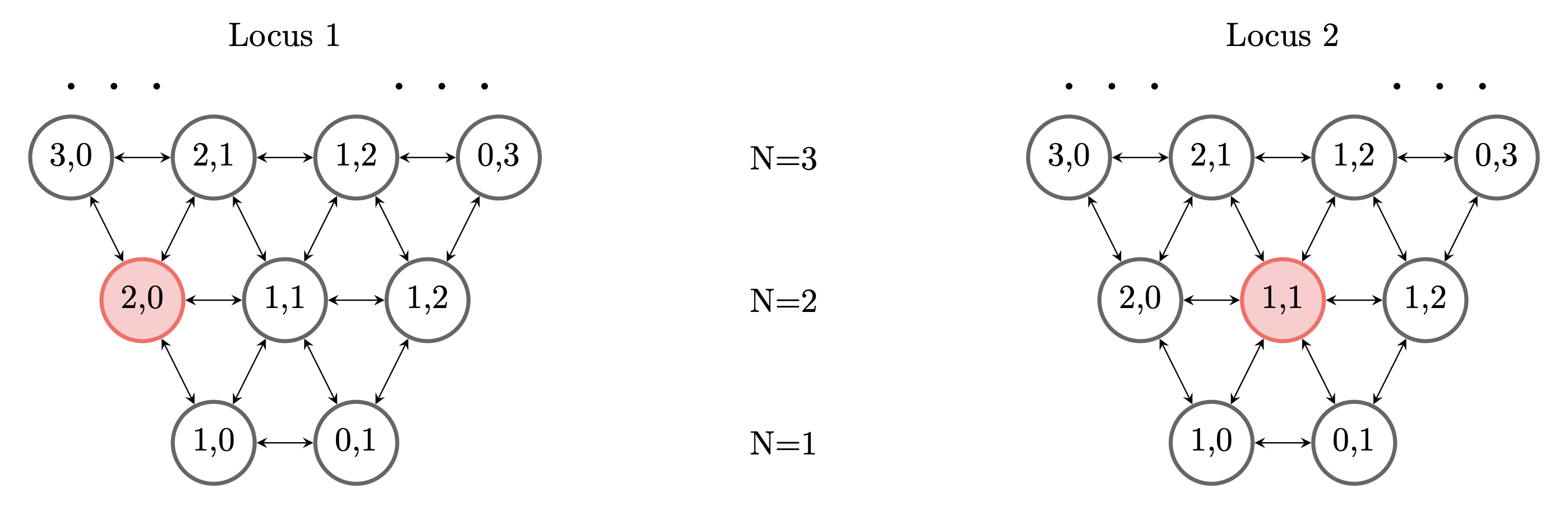
Figure 1: Graphical representation of the nodes identifying the states of the dual and the mixture components of the filtering distributions.

Note that, at least in principle, one could extend the strategy laid out in Barbour et al. (2000) for exploiting duality in order to identify an expansion for the diffusion transition function. This goal however entails a non trivial adaptation of their methodology and is left for future work.

Next we turn to the marginal smoothing problem. When further observations become available at a later time, sometimes it is useful to improve previous estimates with the additional data. This procedure typically results in smoother estimates, whence the name. Determining the smoothing distribution at time $t_{i}$ requires in general integrating out the signal trajectory at all other times, conditional on the entire dataset. This calculation is typically unfeasible, but duality provides an efficient way of identifying the quantities of interest.

Proposition 3.2.

For $0\leq i\leq n-1$, the marginal smoothing density of $\mathbf{X}(t_{i})$ given $\mathbf{Y}(t_{0}),\ldots,\mathbf{Y}(t_{n})$ admits representation

$$\mathbf{X}(t_{i})|\mathbf{Y}(t_{0}),\ldots,\mathbf{Y}(t_{n})\sim\sum_{\mathbf{m},\mathbf{n}>\mathbf{0}}w_{i}(\mathbf{m},\mathbf{n})p_{\boldsymbol{\alpha}+\mathbf{m}+\mathbf{n},\boldsymbol{\sigma},\mathbf{J}}(\mathrm{d}\mathbf{x}),$$ (17)

where, for $\hat{c}_{i}(\mathbf{n})$ as in Proposition 3.1,

$$w_{i}(\mathbf{m},\mathbf{n})\propto C_{\mathbf{m},\mathbf{n}}\omega_{i+1}(\mathbf{m})\hat{c}_{i}(\mathbf{n}),\quad\quad C_{\mathbf{m},\mathbf{n}}=\frac{k(\mathbf{m})k(\mathbf{n})}{k(\mathbf{m}+\mathbf{n})},$$ (18)

$$\omega_{i+1}(\mathbf{m})=\sum_{\mathbf{n}>\mathbf{0}}\omega_{i+2}(\mathbf{n})d_{i+1}(\mathbf{n},\mathbf{y}(t_{i+1}))p_{\mathbf{n}+\mathbf{y}(t_{i+1}),\mathbf{m}}(t_{i+1}-t_{i}),$$ (19)

with $d_{i+1}(\cdot,\cdot)$ and $p_{\cdot,\cdot}(t)$ as in Proposition 3.1.

Proof.

Bayes’ Theorem and conditional independence allow to write, for every $0\leq i\leq n-1$,

$$p(\mathbf{X}(t_{i})|\mathbf{Y}(t_{0}),\ldots,\mathbf{Y}(t_{n}))\propto p(\mathbf{Y}(t_{i+1}),\ldots,\mathbf{Y}(t_{n})|\mathbf{X}(t_{i}))p(\mathbf{X}(t_{i})|\mathbf{Y}(t_{0}),\ldots,\mathbf{Y}(t_{i}))$$

where the last factor is given in Proposition 3.1. It can be now shown by induction that

$$\mathbf{Y}(t_{i+1}),\ldots,\mathbf{Y}(t_{n})|\mathbf{X}(t_{i})\sim\sum_{\mathbf{m}>\mathbf{0}}\omega_{i+1}(\mathbf{m})h(\mathbf{x},\mathbf{m}).$$ (20)

Indeed, (20) holds for $i=n-1$ since (12) implies

$$\text{MN}_{L}(\mathbf{y};\mathbf{N}_{n},\mathbf{x})=h(\mathbf{x},\mathbf{y})d_{n}(\mathbf{0},\mathbf{y}),$$

and $\mathbb{E}\left[h(\mathbf{X}(t_{n}),\mathbf{m})\mid\mathbf{X}(t_{n-1})=\mathbf{x}^{\prime}\right]$ can be written in terms of the dual transition probabilities, as done in the proof of Proposition 3.1. Assume then (20) holds for $i+1$, and note that $\mathbf{Y}(t_{i+1}),\ldots,$ $\mathbf{Y}(t_{n})|\mathbf{X}(t_{i})$ has law

$$\int_{\Delta} \text{MN}_{L}(\mathbf{y}(t_{i+1});\mathbf{N}_{i+1},\mathbf{x}(t_{i+1}))p(\mathbf{y}(t_{i+2}),\ldots,\mathbf{y}(t_{n})|\mathbf{x}(t_{i+1}))P_{t_{i+1}-t_{i}}\left(\mathbf{x}(t_{i}),\mathrm{d}\mathbf{x}(t_{i+1})\right).$$

Since now $h(\mathbf{x},\mathbf{m})\text{MN}_{L}(\mathbf{y};\mathbf{N}_{n},\mathbf{x})=h(\mathbf{x},\mathbf{m}+\mathbf{y})d_{n}(\mathbf{m},\mathbf{y})$ holds for all $\mathbf{x}\in\Delta$ and $\mathbf{m}\in\mathbb{N}^{K}\setminus\left\{0\right\}$, (20) follows from the expansion of the conditional expectation with respect to the dual transition probabilities, upon rearranging the terms. Furthermore, $h$ in (9) satisfies

$$h(\mathbf{x},\mathbf{m})h(\mathbf{x},\mathbf{n})=\frac{k(\mathbf{m})k(\mathbf{n})}{k(\mathbf{m}+\mathbf{n})}h(\mathbf{x},\mathbf{m}+\mathbf{n}),$$ (21)

for all $\mathbf{x}\in\Delta$, $\mathbf{m},\mathbf{n}\in\mathbb{N}^{K}\setminus\left\{0\right\}$. Hence the law of $\mathbf{X}(t_{i})|\mathbf{Y}(t_{0}),\ldots,\mathbf{Y}(t_{n})$ is proportional to

$$\sum_{\mathbf{m}>\mathbf{0}} \omega_{i+1}(\mathbf{m})h(\mathbf{x},\mathbf{m})\sum_{\mathbf{n}>\mathbf{0}}\hat{c}_{i}(\mathbf{n})h(\mathbf{x},\mathbf{n})p_{\boldsymbol{\alpha},\boldsymbol{\sigma},\mathbf{J}}(\mathrm{d}\mathbf{x})$$

$$=\sum_{\mathbf{m}>\mathbf{0}}\sum_{\mathbf{n}>\mathbf{0}}\omega_{i+1}(\mathbf{m})\hat{c}_{i}(\mathbf{n})C_{\mathbf{m},\mathbf{n}}h(\mathbf{x},\mathbf{m}+\mathbf{n})p_{\boldsymbol{\alpha},\boldsymbol{\sigma},\mathbf{J}}(\mathrm{d}\mathbf{x})$$

$$=\sum_{\mathbf{m}>\mathbf{0}}\sum_{\mathbf{n}>\mathbf{0}}\omega_{i+1}(\mathbf{m})\hat{c}_{i}(\mathbf{n})C_{\mathbf{m},\mathbf{n}}p_{\boldsymbol{\alpha}+\mathbf{m}+\mathbf{n},\boldsymbol{\sigma},\mathbf{J}}(\mathrm{d}\mathbf{x}),$$

which, upon normalization, leads to the claim. ∎

4 Implementation and illustration

Propositions 3.1 and 3.2 provide recursion for reweighing the mixture components in order to evaluate the filtering and marginal smoothing distributions given the available data. Algorithm 1 lays out the pseudocode for calculating the filtering mixtures as in Proposition 3.1, while Algorithm 2 does the same for the smoothing mixtures as in Proposition 3.2.

Data: $\mathbf{y}(j)=(\mathbf{y}^{(1)}(t_{j}),\ldots,\mathbf{y}^{(L)}(t_{j}))$ and $t_{j}$ for $j=0,1,\ldots n$

Set parameters $\boldsymbol{\alpha},\boldsymbol{\sigma}$ and $\mathbf{J}$ for $p_{\boldsymbol{\alpha},\boldsymbol{\sigma},\mathbf{J}}(\mathrm{d}\mathbf{x})$

[0mm] Initialise

       For $\mathbf{m}>\mathbf{0}$

             Compute $c_{0}(\mathbf{m})=p_{\mathbf{y}(t_{0}),\mathbf{m}}(t_{1}-t_{0})$

      

For $j=1,\ldots,n-1$

       Update

             Get $\mathbf{y}(t_{j})$

             For $\mathbf{m}>\mathbf{0}$

                   Compute $d_{j}(\mathbf{m},\mathbf{y}(t_{j}))$

                   $a(\mathbf{m})\leftarrow c_{j-1}(\mathbf{m})\cdot d_{j}(\mathbf{m},\mathbf{y}(t_{j}))$

            

             For $\mathbf{m}>\mathbf{0}$

                   $\hat{c}_{j}(\mathbf{m})\leftarrow\frac{a(\mathbf{m})}{\sum_{\mathbf{m}>\mathbf{0}}a(\mathbf{m})}$

            

      

       Prediction

             For $\mathbf{n}>\mathbf{0}$

                   $c_{j}(\mathbf{n})\leftarrow\sum_{\mathbf{m}>\mathbf{0}}\hat{c}_{j}(\mathbf{m})\cdot p_{\mathbf{m}+\mathbf{y}(t_{j}),\mathbf{n}}(t_{j+1}-t_{j})$

            

      

Last update

       Get $\mathbf{y}(t_{n})$

       For $\mathbf{m}>\mathbf{0}$

             Compute $d_{n}(\mathbf{m},\mathbf{y}(t_{n}))$

             $a(\mathbf{m})\leftarrow c_{n-1}(\mathbf{m})\cdot d_{n}(\mathbf{m},\mathbf{y}(t_{n}))$

      

       For $\mathbf{m}>\mathbf{0}$

             $\hat{c}_{n}(\mathbf{m})\leftarrow\frac{a(\mathbf{m})}{\sum_{\mathbf{m}>\mathbf{0}}a(\mathbf{m})}$

      

Return $\hat{c}_{n}(\mathbf{m})$

Algorithm 1 Evaluation of the mixture weights $\hat{c}_{n}(\mathbf{m})$ in Proposition 3.1

Data: $\mathbf{y}(j)=(\mathbf{y}^{(1)}(t_{j}),\ldots,\mathbf{y}^{(L)}(t_{j}))$ and $t_{j}$ for $j=0,1,\ldots,n$

Set parameters $\boldsymbol{\alpha},\boldsymbol{\sigma}$ and $\mathbf{J}$ for $p_{\boldsymbol{\alpha},\boldsymbol{\sigma},\mathbf{J}}(\mathrm{d}\mathbf{x})$

[0mm] Initialise

       For $\mathbf{m}>\mathbf{0}$

             Obtain $\hat{c}_{j}(\mathbf{m})$ for $j=0,1,\ldots n$ from Algorithm 1

             Compute $c^{*}_{n-1}(\mathbf{m})=p_{\mathbf{y}(n),\mathbf{m}}(t_{n+1}-t_{n})$

      

For $j=n-1,\ldots,1$

       Update

             Get $\mathbf{y}(t_{j})$

             For $\mathbf{m}>\mathbf{0}$

                   Compute $d_{j}(\mathbf{m},\mathbf{y}(t_{j}))$

                   $\omega_{j+1}(\mathbf{m})\leftarrow c^{*}_{j}(\mathbf{m})\cdot d_{j}(\mathbf{m},\mathbf{y}(t_{j}))$

            

      

       Prediction

             For $\mathbf{n}>\mathbf{0}$

                   $c^{*}_{j-1}(\mathbf{n})\leftarrow\sum_{\mathbf{m}>\mathbf{0}}\hat{c}_{j}(\mathbf{m})\cdot p_{\mathbf{m}+\mathbf{y}(j-1),\mathbf{n}}(t_{j}-t_{j-1})$

            

      

Last update

       Get $\mathbf{y}(0)$

       For $\mathbf{m}>\mathbf{0}$

             Compute $d_{0}(\mathbf{m},\mathbf{y}(t_{0}))$

             $\omega_{1}(\mathbf{m})\leftarrow c^{*}_{0}(\mathbf{m})\cdot d_{0}(\mathbf{m},\mathbf{y}(t_{0}))$

      

For $j=0,\ldots,n-1$

       For $\mathbf{m},\mathbf{n}>\mathbf{0}$

             $a(\mathbf{m},\mathbf{n})\leftarrow C_{\mathbf{m},\mathbf{n}}\omega_{j+1}(\mathbf{n})\hat{c}_{j}(\mathbf{m})$

      

       For $\mathbf{m},\mathbf{n}>\mathbf{0}$

             $w_{j}(\mathbf{m},\mathbf{n})\leftarrow\frac{a(\mathbf{m},\mathbf{n})}{\sum_{\mathbf{m},\mathbf{n}>\mathbf{0}}a(\mathbf{m},\mathbf{n})}$

      

Return $w_{j}(\mathbf{m},\mathbf{n})$ for $j=0,\ldots,n-1$

Algorithm 2 Evaluation of the mixture weights $w_{i}(\mathbf{m},\mathbf{n})$ in Proposition 3.2

The concrete implementation of these algorithm must however deal with two key hurdles. The first is the fact that the normalising constant in (6) and the constant $k(\mathbf{m})$ in (9) involve integrals which are not available in closed form. Aurell et al. (2019) and Favero et al. (2021) derive a series representation of the normalising constant $Z$ when $\boldsymbol{\sigma}=0$ by involving the Kummer (confluent hypergeometric) function. In general, these integrals need to be approximated with appropriate methods. This hurdle carries over to the evaluation of the marginal distributions $d_{n}(\mathbf{m},\mathbf{y})$ (cf. Propositions 3.1-3.2), as one can check that

$$d_{n}(\mathbf{m},\mathbf{y})=\prod_{l=1}^{L}\left(\dfrac{N^{(l)}_{n}!}{\prod_{i=1}^{K_{l}}y_{i}^{(l)}!}\right)\frac{\tilde{C}(\mathbf{m}+\mathbf{y})}{\tilde{C}(\mathbf{m})}$$ (22)

where

$$\tilde{C}(\mathbf{m}):=\int_{\Delta}\mathbf{x}^{\mathbf{m}+\boldsymbol{\alpha}-1}e^{2V(\mathbf{x};\boldsymbol{\sigma},\mathbf{J})}\mathrm{d}\mathbf{x}$$ (23)

is in general not available. Here we adopt a naive Monte Carlo sampler, as Monte Carlo approximations typically outperform quadrature methods in high dimensions, particularly in terms of computational efficiency and ease of implementation, at the cost of higher variability in accuracy. Concretely, $Z$ in (6) is approximated by drawing $B$ iid samples $\mathbf{x}^{(b)}$ from $\pi_{\boldsymbol{\alpha}}$ and computing $B^{-1}\sum_{b=1}^{B}e^{2V_{\boldsymbol{\sigma},\mathbf{J}}(\mathbf{x}^{(b)})}$. The other needed functionals can be computed similarly.

The second difficulty arises in handling the dual process $\mathbf{M}$, as no closed formula for its transition probabilities is available. Here we adopt the strategy used in Kon Kam King et al. (2024), whereby the transition probabilities are approximated by means of several simulated trajectories of the dual. More precisely, one runs multiple times the jump process starting in $\mathbf{m}$ over the needed time interval, and the transition probability $p_{\mathbf{m},\mathbf{n}}(\Delta t)$ is then approximated by the empirical distribution over the arrival points $\mathbf{n}$. This procedure is repeated for every starting point $\mathbf{m}$ with positive mass in the last available mixture, and then the probability masses over the arrival points are aggregated appropriately. The simulation of each run of the dual process is conducted using the Gillespie algorithm (Gillespie, 2001), which alternates drawing exponential holding times and jumps of the embedded chain until the time interval is exhausted. This strategy, besides being easy to implement, has the additional advantage of automatically reducing the cardinality of the transition probability support, which is countable, to a finite set. This corresponds to the support of the empirical distribution obtained as explained above, where the Monte Carlo runs of the dual process place probability mass in the most important part of the state space, in accordance to the dual process dynamics.

Additionally, we adopt a pruning strategy, which was discussed in Kon Kam King et al. (2021). This consists in retaining only the points of the above simulation which are assigned probability mass above a desired threshold, or the points with decreasingly ranked probability mass which collectively provide mass over a desired threshold. Its application is straightforward and, despite not being necessary, makes the implementation more efficient.

To illustrate, we compute the filtering distributions for a two-locus two-allele setting, i.e., when $L=K_{1}=K_{2}=2$, as in Figure 1. We assume pairwise interactions occur according to the rate matrix

$$\mathbf{J}=\begin{pmatrix}0&0&J_{1}&0\\ 0&0&0&J_{2}\\ J_{1}&0&0&0\\ 0&J_{2}&0&0\\ \end{pmatrix}$$ (24)

and within-locus selection is determined by $\boldsymbol{\sigma}$. We simulate a c-WF trajectory with $\boldsymbol{\alpha}=(1.8,1.4,1.9,$ $1.7)$, $\boldsymbol{\sigma}=(0.5,0,0,1.2)$, $J_{1}=0.9$, and $J_{2}=1.8$, by using an approximating Markov chain as in Aurell et al. (2019), leveraging on their scaling limit.

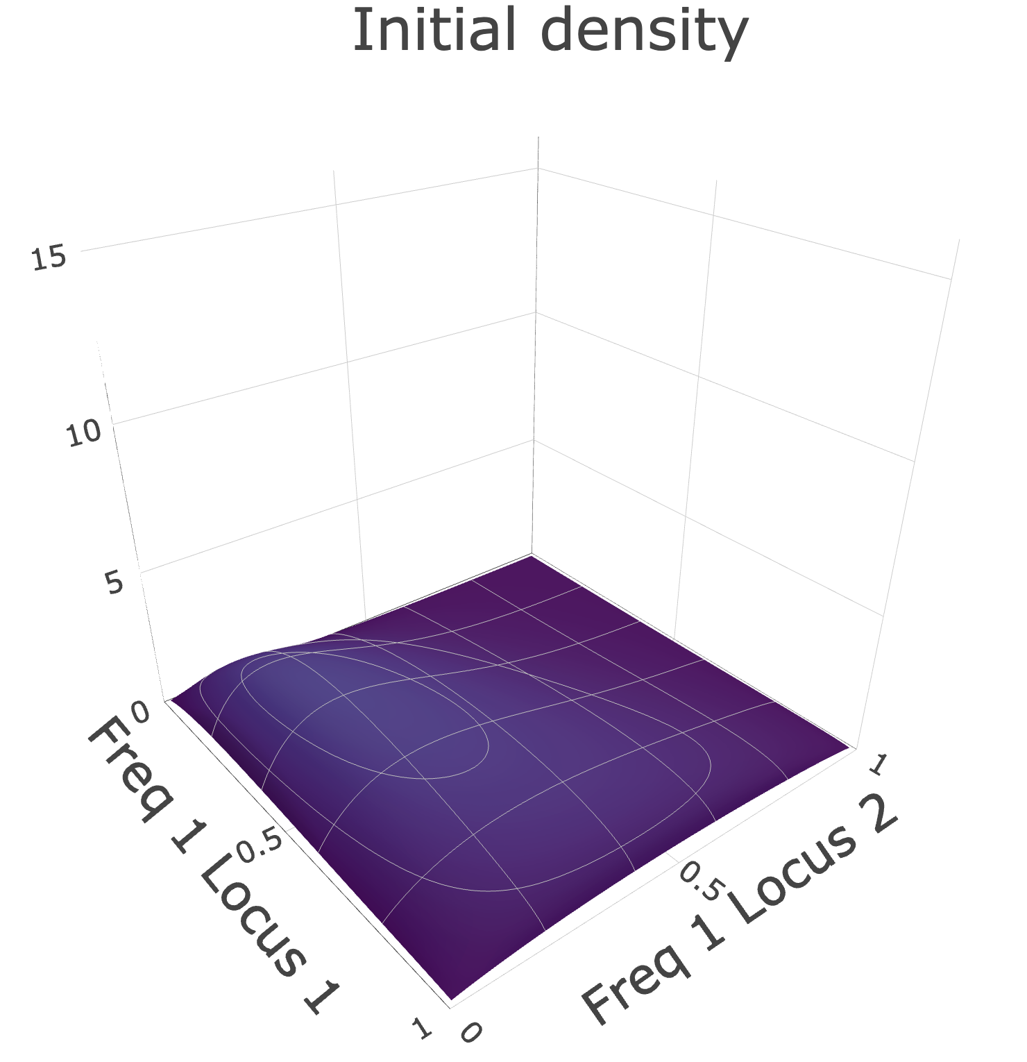
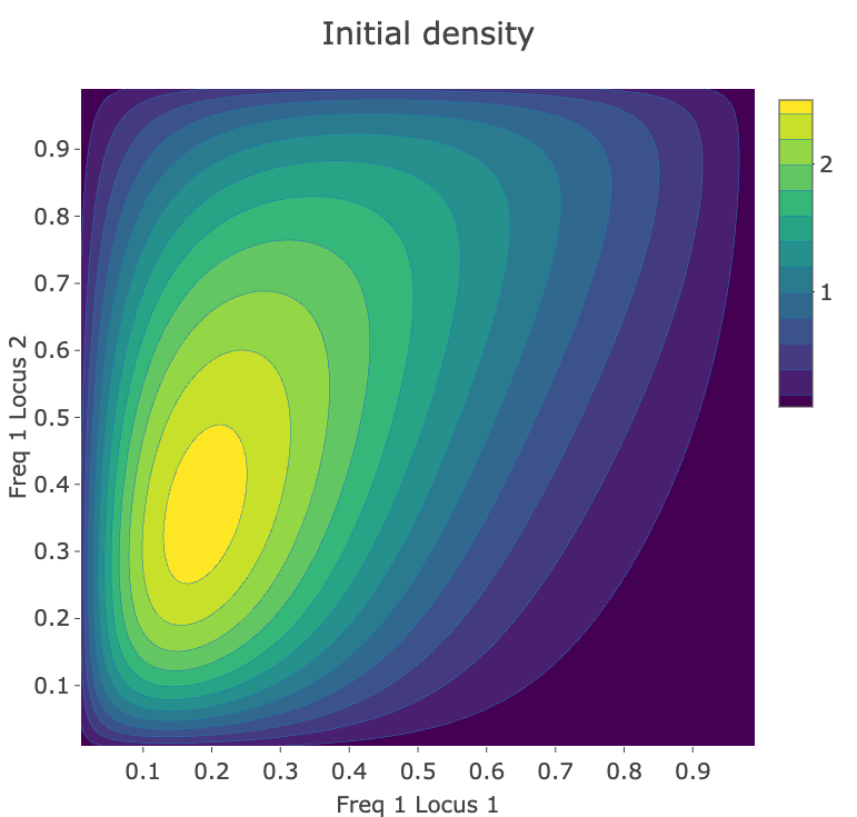
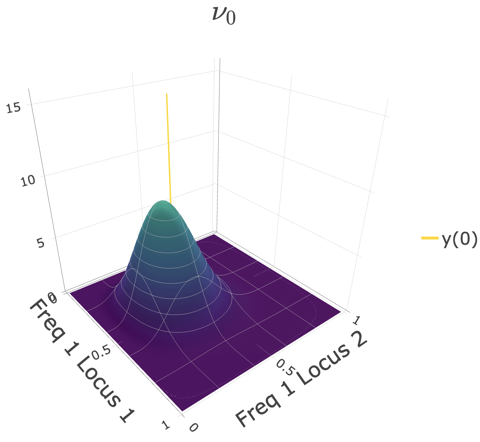
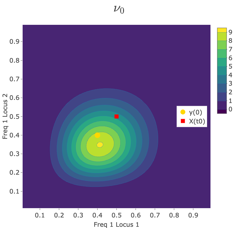
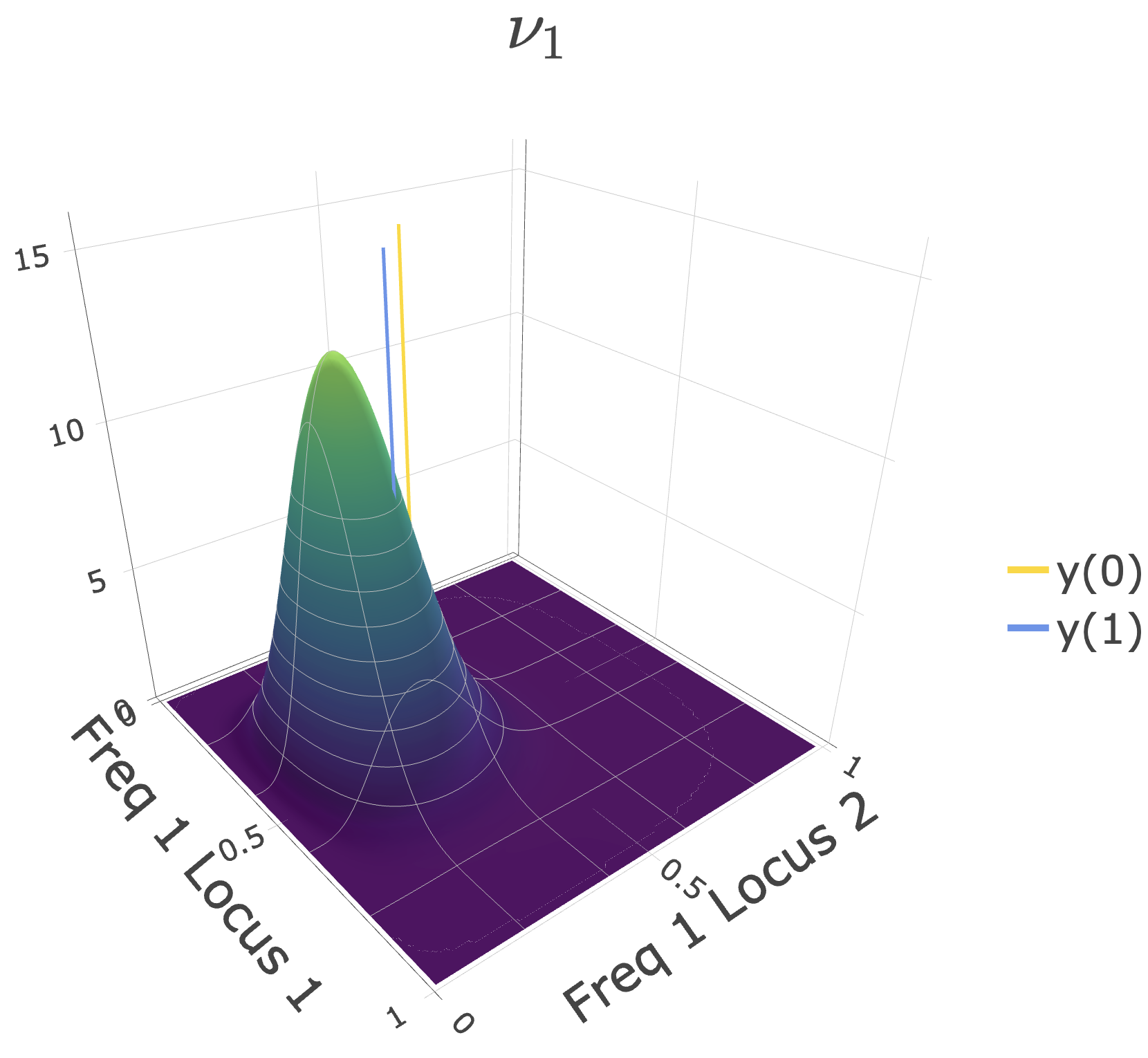
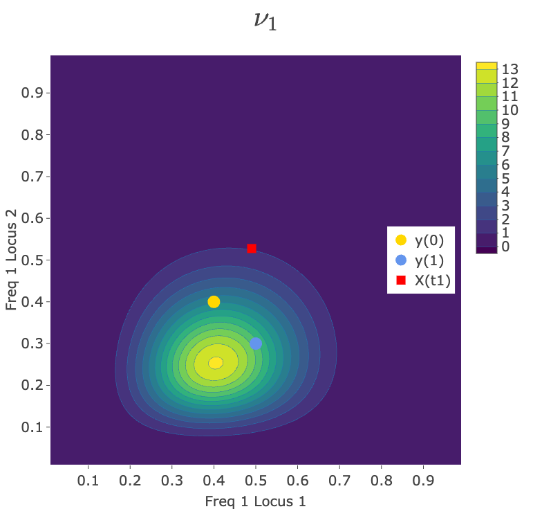
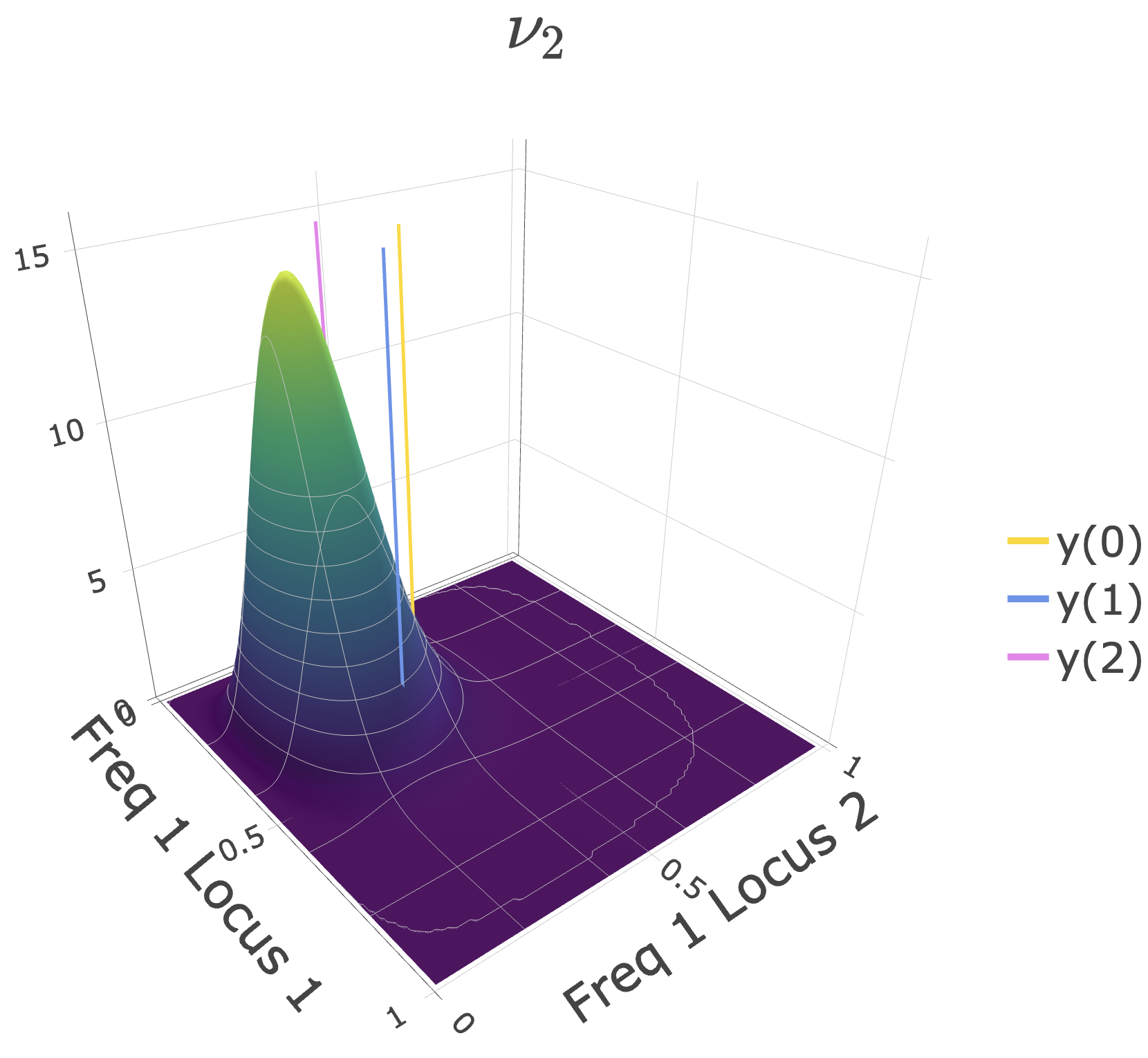
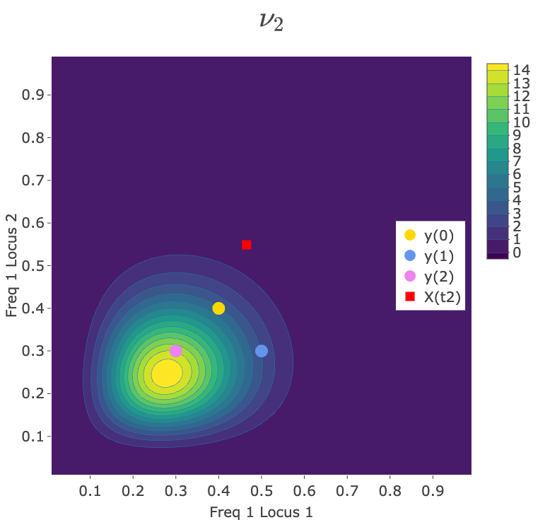
Figure 2: 3D-plots and contours for the initial density (top row) and the filtering distributions $\nu_{n}$ for $n=0,1,2$. Bars (left) and dots (right) indicate the data (transformed into relative frequencies), the square (right) indicated the true signal value.

Figure 2 displays the initial density and the filtering distributions at three consecutive time points, for data values given by (4,6,4,6), (5,5,3,7), and (3,7,3,7), respectively. In the top row, the initial distribution, before collecting any data, is fairly well spread on the state space, with a slight skew towards lower frequencies of type 1 at either locus. The subsequent three rows illustrate the filtering distributions computed according to the strategy outlined in Proposition 3.1, using a naive Monte Carlo approximation of the required normalising constant and a Gillespie-based approximation of the dual process transition probabilities. Bars in left plots and dots in right plots indicate the data, transformed into relative frequencies of type 1, while the red square indicates the true signal value. The Figure shows how the filtering distribution uses the information present in the data to move the mass towards regions of the state space where the signal is believed to be.

The approach to computing the filtering and smoothing distributions described and illustrated here is not limited to this specific example, but can in principle be applied to any parameterization of the model considered in this paper, for any number of types and loci. The filtering and smoothing distributions obtained through this method can then be used to derive estimators for the signal values at the time points of interest, as well as an approximate representation of the likelihood given a dataset which in turn is the basis for parameter inference. A comprehensive investigation of full inference for this model, together with an evaluation of the algorithm’s performance, remain topics of great interest, which we leave for future work.

Declarations

The authors have no competing interests to declare that are relevant to the content of this article.

References

- Ascolani et al. (2021) Ascolani, F., Lijoi, A. and Ruggiero, M. (2021). Predictive inference with Fleming–Viot-driven dependent Dirichlet processes. Bayesian Anal. 16, 371–395.
- Ascolani et al. (2023) Ascolani, F., Lijoi, A. and Ruggiero, M. (2023). Smoothing distributions for conditional Fleming–Viot and Dawson–Watanabe diffusions. Bernoulli 29, 1410-1434.
- Ascolani et al. (2024) Ascolani, F., Damato, S. and Ruggiero, M. (2024). An R package for nonparametric inference on dynamic populations with infinitely many types. J. Comput. Biol, to appear.
- Aurell et al. (2019) Aurell, E., Ekeberg, M. and Koski, T. (2019). On a multilocus Wright–Fisher model with mutation and a Svirezhev-Shahshahani gradient-like selection dynamics. arXiv:1906.00716.
- Bain and Crisan (2009) Bain, A. and Crisan, D. (2009). Fundamentals of stochastic filtering. Springer.
- Barbour et al. (2000) Barbour, A.D., Ethier, S. and Griffiths, R.C. (2000). A transition function expansion for a diffusion model with selection. The Annals of Applied Probability 10, 123–162.
- Cappé et al. (2005) Cappé, O., Moulines, E. and Rydén, T. (2005). Inference in hidden Markov models. Springer.
- Chaleyat-Maurel and Genon-Catalot (2006) Chaleyat-Maurel, M. and Genon-Catalot, V. (2006). Computable infinite-dimensional filters with applications to discretized diffusion processes. Stochastic Process and their Application 116, 1447–1467.
- Chaleyat-Maurel and Genon-Catalot (2009) Chaleyat-Maurel, M. and Genon-Catalot, V. (2009). Filtering the Wright–Fisher diffusion. ESAIM Probab. Stat. 13, 197–217.
- Dawson (1993) Dawson, D.A. (1993). Measure-valued Markov processes. Ecole d’Eté de Probabilités de Saint Flour XXI. Lecture Notes in Mathematics 1541. Springer, Berlin.
- Dawson and Greven (1999) Dawson, D.A. and Greven, A. (1999). Hierarchically interacting Fleming–Viot processes with selection and mutation: multiple space time scale analysis and quasi-equilibria. Electron. J. Probab. 1, 1–84.
- Dawson et al. (1995) Dawson, D.A., Greven, A. and Vaillancourt, J. (1995). Equilibria and quasi-equilibria for infinite collections of interacting Fleming–Viot processes. Trans. Amer. Math. Soc. 347, 7, 2277–2360.
- Etheridge (2009) Etheridge, A.M. (2009). Some mathematical models from population genetics. École d’été de Probabilités de Saint-Flour XXXIX. Lecture Notes in Math. 2012. Springer.
- Etheridge and Griffiths (2009) Etheridge, A.M. and Griffiths, R.C. (2009). A coalescent dual process in a Moran model with genic selection. Theoretical population biology 75, 320–330.
- Ethier and Griffiths (1993) Ethier, S.N. and Griffiths, R.C. (1993). The transition function of a Fleming–Viot process. Ann. Probab. 21, 1571–1590.
- Ethier and Kurtz (1981) Ethier, S.N. and Kurtz, T.G. (1981). The infinitely-many-neutral-alleles diffusion model. Adv. Appl. Probab. 13, 429–452.
- Ethier and Kurtz (1986) Ethier, S.N. and Kurtz, T.G. (1986). Markov processes. Characterization and Convergence. Wiley, New York.
- Ethier and Nagylaki (1989) Ethier, S.N. and Nagylaki, T. (1989). Diffusion approximations of the two-locus Wright–Fisher model. J. Math. Biol. 27, 17–28.
- Ewens (1979) Ewens, W.J. (1979). Mathematical population genetics. Springer-Verlag, Berlin.
- Ewens (2004) Ewens, W.J. (2004). Mathematical Population Genetics. I. Theoretical Introduction, 2nd Edition, Interdisciplinary Applied Mathematics, Springer-Verlag, New York, Vol. 27.
- Favero et al. (2021) Favero, M., Hult, H. and Koski, T. (2021). A dual process for the coupled Wright–Fisher diffusion. Journal of Mathematical Biology 82, 1–29.
- Feng (2010) Feng, S. (2010). The Poisson–Dirichlet distribution and related topics. Springer, Heidelberg.
- Fukushima and Stroock (1986) Fukushima, M. and Stroock, D. (1986). Reversibility of solutions to martingale problems. Probability, statistical mechanics, and number theory, 9, 107–123.
- García-Pareja et al. (2021) García-Pareja, C., Hult, H. and Koski, T. (2021). Exact simulation of coupled Wright–Fisher diffusions. Adv. Appl. Probab. 53, 923–950.
- Gillespie (2001) Gillespie, D.T. (2001). Stochastic simulation of chemical kinetics. Annu. Rev. Phys. Chem. 58, 35–55.
- Greven et al. (2001) Greven, A., Klenke, A. and Wakolbinger, A. Interacting Fisher–Wright diffusions in a catalytic medium. Probab. Theory Relat. Fields 120 85–117.
- Greven et al. (2005) Greven, A., Limic, V. and Winter, A. (2005). Representation theorems for interacting Moran models, interacting Fisher–Wright diffusions and applications. Electron. J. Probab. 10, 1286–1358.
- Griffiths et al. (2019) Griffiths, R.C., Jenkins, P.A. and Lessar,d S. (2019). Corrigendum to “A coalescent dual process for a Wright-Fisher diffusion with recombination and its application to haplotype partitioning” [Theor. Popul. Biol. 112 (2016) 126–138]. Theoretical Population Biology, 130, 203–203.
- Griffiths et al. (2024) Griffiths, R.C., Ruggiero, M., Spanò, D. and Zhou, Y. (2024). Dual process in the two-parameter Poisson-Dirichlet diffusion. Stoch. Proc. Appl. 179, 104500.
- Jansen and Kurt (2014) Jansen, S. and Kurt, N. (2014). On the notion(s) of duality for Markov processes. Probab. Surv. 11, 59–120.
- Kon Kam King et al. (2021) Kon Kam King, G., Papaspiliopoulos, O. and Ruggiero, M. (2021). Exact inference for a class of hidden Markov models on general state spaces. Electron. J. Stat. 15, 2832–2875.
- Kon Kam King et al. (2024) Kon Kam King, G., Pandolfi, A., Piretto, M. and Ruggiero, M. (2024). Approximate filtering via discrete dual processes. Stoch. Proc. Appl. 168, 104268.
- Maruyama (1977) Maruyama, T. (1977). Stochastic problems in population genetics (Vol. 17). Springer-Verlag Berlin Heidelberg.
- Papaspiliopoulos and Ruggiero (2014) Papaspiliopoulos, O. and Ruggiero, M. (2014). Optimal filtering and the dual process. Bernoulli 20, 1999–2019.
- Papaspiliopoulos et al. (2016) Papaspiliopoulos, O., Ruggiero, M. and Spanò, D. (2016). Conjugacy properties of time-evolving Dirichlet and gamma random measures. Electron. J. Stat. 10, 3452–3489.
- Pruenster and Ruggiero (2013) Pruenster, I. and Ruggiero, M. (2013). A Bayesian nonparametric approach to modeling market share dynamics. Bernoulli 19, 64–92.
- Vaillancourt (1990) Vaillancourt, J. (1990). Interacting Fleming-Viot processes. Stochastic Process. Appl. 1, 45–57.