Exponentially-enhanced quantum sensing with many-body phase transitions

Abstract

Quantum sensors based on critical many-body systems are known to exhibit enhanced sensing capability. Such enhancements typically scale algebraically with the probe size. Going beyond algebraic advantage and reaching exponential scaling has remained elusive when all the resources, such as the preparation time, are taken into account. In this work, we show that systems with first order quantum phase transitions can indeed achieve exponential scaling of sensitivity, thanks to their exponential energy gap closing. Remarkably, even after considering the preparation time using local adiabatic driving, the exponential scaling is sustained. Our results are demonstrated through comprehensive analysis of three paradigmatic models exhibiting first order phase transitions, namely Grover, $p$-spin, and biclique models. We show that this scaling survives moderate decoherence during state preparation and also can be optimally measured in experimentally available basis.

I Introduction

Quantum sensing is an important component of quantum technologies due to its potential for developing a new generation of probes, capable of environmental monitoring with unprecedented precision beyond classical sensors Degen et al. (2017); Braun et al. (2018); Ye and Zoller (2024). In this context, the sensitivity of a probe can be quantified by Fisher information, inverse of which puts a bound on the uncertainty of the estimation protocol Braunstein and Caves (1994); Paris (2009). In classical sensors, Fisher information, at best, scales linearly with resources, such as the system size $L$ (standard limit). Quantum features may result in super-linear scaling of Fisher information, known as quantum enhanced sensitivity. This has been discovered in a series of seminal works by Giovannetti et al., where they showed that a special form of entangled states, known as the Greenberger–Horne–Zeilinger (GHZ) states, can be used to estimate the phase imprinted by a unitary operation with Fisher information scaling as $L^{2}$ (Heisenberg limit) Giovannetti et al. (2004, 2006, 2011). In the presence of $k$-body interactions in the generator of the unitary operation, the sensitivity can be further enhanced to $L^{2k}$ Boixo et al. (2007). In a fundamentally different approach, quantum enhanced sensitivity has also been identified in many-body systems when they go through a quantum phase transition. This includes, first-order Raghunandan et al. (2018); Mirkhalaf et al. (2020); Yang and Jacob (2019); Heugel et al. (2019), second-order  Zanardi and Paunković (2006); Zanardi et al. (2007, 2008); Invernizzi et al. (2008); Gu (2010); Gammelmark and Mølmer (2011); Skotiniotis et al. (2015); Rams et al. (2018); Chu et al. (2021); Liu et al. (2021); Montenegro et al. (2021), Floquet Mishra and Bayat (2021, 2022), time crystal Montenegro et al. (2023); Iemini et al. (2024); Yousefjani et al. (2024a); Gribben et al. (2024), Stark He et al. (2023); Yousefjani et al. (2024b, 2023) and quasi-periodic Sahoo et al. (2024) localization, and topological Sarkar et al. (2022, 2024) phase transitions. In all these critical systems, where Fisher information scales algebraically as $L^{\beta}$ (with $\beta>1$), the many-body system goes through an algebraic energy gap closing in its spectrum. This gives rise to the conjecture that energy gap closing might be the reason behind quantum enhanced sensitivity Montenegro et al. (2024). Non-equilibrium quench dynamics in many-body systems have also been explored for achieving quantum-enhanced sensitivity in which Fisher information also depends on evolution-time $t$ and typically scales as $t^{2}L^{\beta}$ Ilias et al. (2022); Manshouri et al. (2024). While in all these cases, Fisher information, and thus the precision, scales algebraically, one may wonder whether quantum features can result in the possibility of even a better quantum advantage, namely exponentially enhanced quantum sensing.

Exponential enhancement has in fact been reported in Ref. Roy and Braunstein (2008), for the GHZ-based sensing protocols where the required entanglement in the initial state demands exponentially large number of unitary gates, making its implementation very challenging. In non-Hermitian systems exponential sensitivity can be achieved in the eigenenergy spectrum at exceptional points (parameter value where multiple eigenvalues and eigenstates coalesce) Wiersig (2014); Chen et al. (2017); Yu et al. (2020); Hodaei et al. (2017); Liu et al. (2016). However, it is debated whether the quantum advantage would survive the quantum noise arising from the non-orthogonality of the eigenstates Langbein (2018); Chen et al. (2019). Proposals based on tight-binding non-Hermitian topological systems have also reported exponential sensitivity McDonald and Clerk (2020); Budich and Bergholtz (2020); Koch and Budich (2022) for inferring the value of a perturbative boundary coupling in the steady state. While these works show great potential for quantum enhancement, the schemes are restrictive for several reasons: (i) the preparation time for the steady state is typically long whose consideration in resource analysis may destroy quantum advantage; (ii) the schemes are limited to driven coupled resonators as non-Hermitian Hamiltonians cannot faithfully describe an open system evolution beyond a short time; and (iii) the necessity for measuring a perturbatively small coupling exclusively at the boundary is also a big constraint. In fact, a fundamental constraint derived in Ref. Ding et al. (2023) show that non-Hermitian sensors cannot perform better than Hermitian counterparts. Therefore, finding a concrete protocol with Hermitian systems showing exponential scaling advantage even when the resources are taken into account is highly desirable.

In this work, we show that it is indeed possible to achieve the exponential scaling for sensitivity by leveraging the first-order phase transitions where the energy gap also closes exponentially in system size. We then show that even if the preparation time of the critical state is taken into account, the exponential sensitivity still prevails. Our results are shown analytically for a paradigmatic model, namely Grover model, and numerically for $p$-spin and a biclique spin model that are prototypical systems from a quantum annealing perspective. This estimation process can be performed in experimentally available measurement basis. We consider the issue of decoherence during state preparation and show that the exponential scaling is sustained up to certain dephasing strength. The local nature of criticality-based sensors is also addressed and an adaptive estimation strategy is sketched out to harness the full advantage of the exponential scaling for arbitrary value of the parameter to be estimated.

II Parameter estimation

In this work, we will be considering single parameter estimation, where the value of an unknown parameter $\theta$ is estimated by performing measurements on a quantum state $\rho(\theta)$ that encodes the parameter. The quantum state is known as the probe state and the measurement outcomes are fed into an estimator function to infer the value of the parameter. In general, the measurement can be described by a complete set of Positive Operator Valued Measurement (POVM) $\{\Pi_{n}\}$ where the $n$th outcome occurs with probability $p_{n}(\theta){=}\text{Tr}\left[\rho(\theta)\Pi_{n}\right]$. The uncertainty of estimating the unknown parameter $\theta$, quantified by standard deviation $\delta\theta$, is bounded through Cramér-Rao inequality $\delta\theta{\geq}1/\sqrt{\mathcal{M}\>F^{C}}$. Here, $\mathcal{M}$ is the total number of measurements and the basis-dependent classical Fisher information (CFI), $F^{C}{=}\sum_{n}p_{n}(\partial_{\theta}\log p_{n})^{2}$ Paris (2009). In order to have a measurement-independent quantity, one can maximize the CFI with respect to all possible measurements to obtain Quantum Fisher Information (QFI) $F^{Q}$, namely $F^{Q}{=}\max_{\{\Pi_{n}\}}F^{C}$. As a result, the Cramér-Rao inequality becomes

$$\delta\theta\geq\frac{1}{\sqrt{\mathcal{M}\>F^{C}}}\geq\frac{1}{\sqrt{\mathcal{M}\>F^{Q}}}\,,$$ (1)

where QFI gives the ultimate precision limit of the estimation. Interestingly, for evaluating the QFI one can avoid the notorious optimization over all possible measurement basis and instead consider the symmetric logarithmic derivative (SLD) operator $\mathcal{L}$, implicitly defined as

$$\frac{\partial\rho(\theta)}{\partial\theta}{=}\frac{\rho(\theta)\mathcal{L}_{\theta}+\mathcal{L}_{\theta}\rho(\theta)}{2}$$ (2)

The QFI is then expressed as $F^{Q}{=}\text{Tr}\left[\rho(\theta)\mathcal{L}^{2}_{\theta}\right]$. For pure states $\rho(\theta){=}\ket{\psi(\theta)}\bra{\psi(\theta)}$, the expressions are simplified to $\mathcal{L}_{\theta}{=}2\partial_{\theta}\rho(\theta)$, and consequently (Paris, 2009)

$$F^{Q}(\theta){=}4\left(\braket{\partial_{\theta}\psi(\theta)}{\partial_{\theta}\psi(\theta)}-|\braket{\partial_{\theta}\psi(\theta)}{\psi(\theta)}|^{2}\right)\,.$$ (3)

As QFI quantifies the rate of change of the probe state, it is also equivalent to the fidelity susceptibility. In the context of the ground state of a Hamiltonian $H(\theta)$, this leads to another expression for QFI You et al. (2007)

$$F^{Q}(\theta){=}4\sum_{n\neq 0}\frac{|\braket{\psi_{n}(\theta)}{\partial_{\theta}H(\theta)}{\psi_{0}(\theta)}|^{2}}{(E_{n}(\theta)-E_{0}(\theta))^{2}}.$$ (4)

Here $\ket{\psi_{n}}$ and $E_{n}$ are the $n$-th eigenvector and eigenvalue of $H(\theta)$. It is worth emphasizing that to achieve the ultimate precision limit, given by the QFI, one has to perform measurement in the optimal basis. The optimal measurement basis is not unique, although one choice is always given by the projectors formed from the eigenvectors of the SLD operator $\mathcal{L}_{\theta}$.

III Models

Quantum many-body systems have been proven to be very useful to serve as quantum sensors achieving quantum enhanced sensitivity in both equilibrium and non-equilibrium scenarios Montenegro et al. (2024). In particular, the ground state of many-body systems across various types of phase transitions have been identified as effective quantum sensors. In such systems the Hamiltonian, in general, has the form

$$H(\theta){=}H_{1}+\theta H_{2},$$ (5)

where $H_{1}$ and $H_{2}$ are two competing terms and $\theta$ is the unknown parameter to be estimated. When the role of competing terms become comparable, say at $\theta=\theta_{c}$, the system may go through a phase transition where the ground state $\ket{\mathrm{GS}(\theta)}$ changes dramatically. From the spectral perspective, the ground state and the first excited state go through an anti-crossing at $\theta=\theta_{c}$ where the energy gap vanishes in the thermodynamic limit. If the energy gap closes exponentially with the system size, then the system goes through a first order phase transition in which the order parameter discontinuously jumps across the transition point. On the other hand, if the energy gap closes algebraically, then the order parameter changes continuously and it is the first derivative that becomes non-analytic at the phase transition. While the capability of utilizing second order phase transitions as effective quantum sensors has been fully characterized Rams et al. (2018), the first order phase transitions have not been completely explored. As we shall see in the following sections, first order phase transitions indeed allow for estimating $\theta$ with exponential sensitivity, quantified by exponential scaling of QFI with the system size. In the following we introduce three paradigmatic models with first order phase transitions, namely Grover, p-spin, and biclique spin systems.

III.1 Grover model

We first consider a system consisting of $L$ qubits which span a Hilbert space of dimension $N{=}2^{L}$. Every qubit configuration can coherently tunnel to another with equal probability, though one specific qubit configuration $\ket{m}$ has a different energy from the rest. In this situation one can write the Hamiltonian,

$$H_{\rm Grover}(\theta) =-\ket{m}\bra{m}-\theta\ket{\psi}\bra{\psi},$$

where

$$\ket{\psi}{=}\frac{1}{\sqrt{N}}\sum_{j=1}^{N}\ket{j}{=}\frac{1}{\sqrt{N}}\ket{m}+\sqrt{\frac{N-1}{N}}\ket{m^{\perp}},$$ (7)

with

$$\ket{m^{\perp}}{=}\frac{1}{\sqrt{N-1}}\sum_{j\neq m}\ket{j}.$$ (8)

One can easily show that the Hamiltonian in Eq. (LABEL:eq:Grover_ham) can be effectively be written as a two level system spanned by $\ket{m}$ and $\ket{m^{\perp}}$ as,

$$H_{\rm Grover}(\theta)=-\begin{pmatrix}\frac{\theta}{N}+1&\frac{\theta\sqrt{N-1}}{N}\\ \frac{\theta\sqrt{N-1}}{N}&\frac{\theta(N-1)}{N}\end{pmatrix}.$$ (9)

This model is analytically tractable and will serve as a robust theoretical foundation for our conclusions. In this representation, the first-order phase can be analytically shown to be occurring at $\theta_{c}{=}1$ Roland and Cerf (2002).

III.2 $p$-spin model

The second model we consider is based on $p$-spin model Gardner (1985), in a system of $L$ qubits, represented by,

$$H_{p\rm-spin}(\theta) =\Big{[}\,-\lambda L^{1-p}\Big{(}\sum_{j=1}^{L}\sigma^{z}_{j}\Big{)}^{p}+(1-\lambda)\,L^{1-k}\Big{(}\sum_{j=1}^{L}\sigma^{x}_{j}\Big{)}^{k}\Big{]}$$

$$-\theta\sum_{j=1}^{L}\sigma^{x}_{j}$$ (10)

where, $p$ and $k$ are integer numbers and $0{\leq}\lambda{\leq}1$ is an external parameter that tune the system to feature either first or second order phase transition. For $\lambda{=}1$, one gets back the traditional $p-$spin model, in which one has a first order phase transition for $p\geq 3$. By choosing increasing values of $p{\geq}3$ for $\lambda{=}1$, it is possible to shift the critical point from $\theta_{c}{=}1.3$ for $p{=}3$ towards $\theta_{c}{=}1$ for $p{\rightarrow}\infty$ which corresponds to the Grover model Jörg et al. (2010). For $\lambda{\neq}1$, we have an additional antiferromagnetic fluctuation term Seki and Nishimori (2012), i.e. the middle term in Eq. (10), which can change the first order phase transition to a second order one. For instance by choosing $\lambda{=}0.1,p{=}5,k{=}2$ one observes a second order quantum phase transition at $\theta_{c}{=}1.8$ Nishimori and Takada (2017). Due to degeneracy issues with even $p$, we shall only consider the odd cases in this work.

III.3 Biclique spin system

Finally, we consider a biclique graph that can be easily implemented on existing quantum hardware and has been utilized in studies of maximum weighted independent set (MWIS) problems Karp (1972); Feinstein et al. (2023); Ghosh et al. (2024). In such graphs, the system is partitioned into two subsystems $A$ and $B$ with $L_{A}$ and $L_{B}$ spins, respectively. We consider $L_{A}{=}L_{B}{+}1$ which means the total system size will be $L{=}2L_{A}+1$. Every spin in the subsystem $A$ interacts with every spin in subsystem $B$ with antiferromagnetic Ising interaction with strength $J$. In addition, the two subsystems are affected by two different uniform magnetic fields $h_{A}$ and $h_{B}$. To induce a competing term the whole system is subjected to a uniform transverse magnetic field. The Hamiltonian can be expressed as Ghosh et al. (2024)

$$H_{\rm Biclique} = \Bigg{[}J\sum_{j_{A}=1}^{L_{A}}\sum_{j_{B}=1}^{L_{B}}\sigma^{z}_{j_{A}}\sigma^{z}_{j_{B}}+h_{A}\sum_{j_{A}=1}^{L_{A}}\sigma^{z}_{j_{A}}+h_{B}\sum_{j_{B}=1}^{L_{B}}\sigma^{z}_{j_{B}}\Bigg{]}$$ (11)

$$+ \theta\sum_{j{=}1}^{L}\sigma^{x}_{j}.$$

By tuning the longitudinal magnetic fields $h_{A}$ and $h_{B}$ one can engineer the emergence of a first order phase transition at different values of $\theta_{c}$.

IV Scaling Analysis

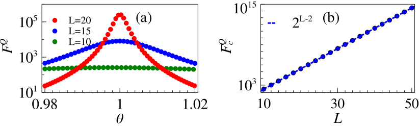
Figure 1: Sensing with Grover model. (a) QFI around the critical point for different system sizes. (c) QFI scaling at criticality ($\theta_{c}{=}1$). The dotted line shows the asymptotic QFI value.

Now we discuss the sensing capabilities of the three models introduced in the previous section to estimate $\theta$ in the ground state due to phase transition. We focus on the scaling of two quantities with respect to the system size. First, we consider the scaling of the energy gap which is necessary to characterize the type of the phase transition. Second, we analyze the scaling of the QFI as a figure of merit for the sensing capability of our models.

IV.1 Sensing with Grover model

For the Grover model, one can obtain the eigenspectrum analytically to compute the energy gap,

$$\Delta(\theta,N){=}\frac{\sqrt{N^{2}(1-\theta^{2})+4N\theta}}{N}.$$ (12)

Note that $N{=}2^{L}$ is the Hilbert space size. The energy gap $\Delta$ has a minimum at $\theta{=}\theta_{c}{=}1$ with $\Delta_{c}{=}\Delta(\theta_{c},N){=}2/\sqrt{N}{=}2^{1-\frac{L}{2}}$. For the ground state of the system one can compute the QFI with respect to $\theta$ which takes the form

$$F^{Q}(\theta)=\frac{4(N-1)}{[N(1-\theta)^{2}+4\theta]^{2}}.$$ (13)

The peak structure of QFI around the critical point is shown in Fig. 1(a). As the system approaches its critical point, the QFI becomes $F^{Q}_{c}{=}F^{Q}(\theta_{c}){=}(N-1)/4\approx 2^{L-2}$ in large $L$ limit. This exponential scaling of $F^{Q}_{c}$ is numerically verified in Fig. 1(b) which shows that the asymptotic behavior is captured by finite number of qubits as well. We also observe the critical exponent for the QFI growth is twice of that for the gap decrease.

IV.2 Sensing with $p$-spin model

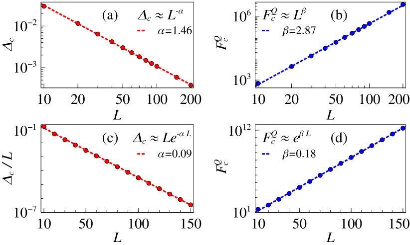
Figure 2: Sensing with $p$-spin model. (a) Energy gap scaling for $p$-spin model (Eq. (10)) for $\lambda{=}0.1,p{=}5,k{=}2$ at criticality occurring near $\theta{=}1.8$. (b) Algebraic QFI scaling at criticality. (c) Energy gap scaling for $\lambda{=}1,p{=}3$ at criticality occurring near $\theta{=}1.3$. (d) Exponential QFI scaling at criticality for this case.

The second model that we consider for sensing is the $p-$spin model, introduced in Eq. (10). In this model, not only the critical point $\theta_{c}$ can be tuned by controlling $p$, $k$, and $\lambda$, but also the nature of phase transition can be controlled. For example, for $p{=}5$ , $k{=}2$ and $\lambda{=}0.1$, the phase transition is of second order type and happens at $\theta_{c}{=}1.8$ Nishimori and Takada (2017). To show this, in Fig. 2(a), we plot the energy gap as function of system size at criticality. As the figure shows, the energy gap closes algebraically, i.e. $\Delta_{c}{\propto}L^{\alpha}$ with $\alpha{\approx}1.46$, signalling the second order nature of the phase transition. The corresponding QFI at the critical point is also plotted as a function of system size $L$ in Fig. 2(b). Clearly, the QFI shows an algebraic scaling i.e. $F^{Q}_{c}{\propto}L^{\beta}$ with $\beta{\approx}2.87$ which is the conventional behavior at the second order quantum phase transitions. Note that we again observe that $\beta{\sim}2\alpha$.

By tuning $\lambda{=}1$ and $p{=}3$ one can observe a first order phase transition at $\theta_{c}{=}1.3$ Jörg et al. (2010). The energy gap in this case is known to close exponentially with a multiplicative correction term, so that $\Delta_{c}{\sim}Le^{-\alpha L}$ Jörg et al. (2010). As shown by the numerical fit in Fig. 2(c), $\alpha{\sim}0.09$. The corresponding ground state QFI at the critical point exponentially grows with $L$, i.e. $F^{Q}_{c}{\sim}e^{\beta L}$ with $\beta{\approx}0.18$, as shown in Fig. 2(d). The relation $\beta{\sim}2\alpha$ can be explained by the equivalence between QFI and fidelity susceptibility in Eq. (4). At criticality, the dominant contribution in the sum on the right hand side of the Eq. (4) comes from the first term (with the first excited state) and the overlap in the numerator were found to be linearly scaling with system size. This cancels the linear multiplicative scaling factor of the gap in the denominator and consequently $\beta{=}2\alpha$.

IV.3 Sensing with biclique spin model

Now we focus on the sensing capacity of the biclique spin model described in Eq. (11). Following the recipe of Refs. Feinstein et al. (2023); Ghosh et al. (2024), we take $h_{A[B]}=\Big{(}L_{B[A]}J-2\frac{W_{A[B]}}{L_{A[B]}}\Big{)}$, with $J{=}1$, $W_{A}{=}0.49J$ and $W_{B}{=}0.5J$. For these choices of parameters, the first order quantum phase transition takes place at $\theta_{c}{\approx}0.05$. In Figure 3(a) we plot the scaling of energy gap at the critical point, namely $\Delta_{c}$, with respect to system size $L$. We observe an exponential falling off $\Delta_{c}{\sim}e^{-\alpha L}$ with exponent $\alpha{\approx}1.43$. Consequently, the corresponding ground state QFI at the critical point exponentially grows with systems size as $F^{Q}_{c}{\sim}e^{\beta L}$ with exponent $\beta{\approx}2.94$, as displayed in Fig. 3(b). The observation of $\beta{\sim}2\alpha$ applies here also.

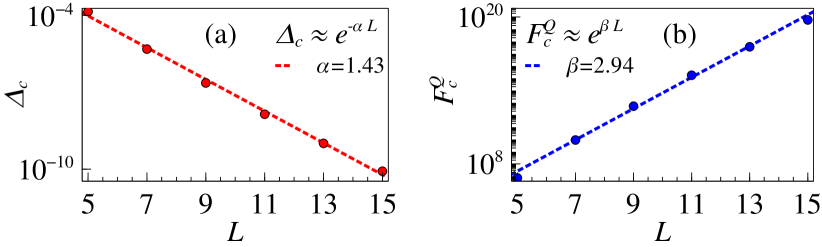
Figure 3: Sensing with biclique model. (a) Energy gap scaling for the biclique spin system (Eq. (11)) at criticality occurring near $\theta_{c}{=}0.05$ with $h_{A[B]}=\Big{(}L_{B[A]}J-2\frac{W_{A[B]}}{L_{A[B]}}\Big{)}$ with $J{=}1$, $W_{A}{=}0.49J$ and $W_{B}{=}0.5J$. (b) QFI scaling at criticality for this system.

V Resource Analysis

So far, we have considered system size as the only resource for sensing. However, since we focus on the ground state QFI, we need to first prepare the ground state of the corresponding Hamiltonians. Typically, there are two ways to prepare a many-body system in its ground state: (i) cooling to ground state; and (ii) adiabatic state preparation. Since the energy gap closes exponentially, both of these methods face severe challenges as cooling will be affected by critical slowing down and adiabatic state preparation requires extremely long preparation times. One may also consider the preparation time as a resource for accomplishing the sensing task. In order to incorporate time into resource analysis one may consider normalized QFI, viz. $F^{Q}/T$ with $T$ being the preparation time, as the right figure of merit for our sensing scheme.

While both cooling and adiabatic state preparation are affected by closing of the energy gap, for sake of simplicity we shall only focus on adiabatic state preparation in this work. The adiabatic theorem states that to prepare the ground state of a many-body system one can start with an easily preparable ground state of a simple Hamiltonian and slowly change the Hamiltonian into the desired one. If the evolution is slow enough, taking place over a long time $T$, then quantum state of the system follows the ground state of the instantaneous Hamiltonian and thus reach the desired ground state at the end of the evolution. The original formulation of the adiabatic theorem requires that $T{\sim}1/\Delta_{{\rm min}}^{2}$ where $\Delta_{{\rm min}}$ is the minimum energy gap of the Hamiltonian throughout the evolution McGeoch (2014). However, there has been a lot of effort to speed up the state preparation Roland and Cerf (2002); Barankov and Polkovnikov (2008); Rezakhani et al. (2009); Grabarits et al. (2024). In fact, it has been demonstrated that one can reach the ground state with high fidelity even if the evolution time only scales as $T{\sim}1/\Delta_{{\rm min}}$ Roland and Cerf (2002).

In order to analyze preparation time in our schemes, we re-parameterize the Hamiltonian in Eq. (5) into the following time-dependent form

$$H(s(t)){=}s(t)H_{1}+(1-s(t))H_{2},$$ (14)

where the parameter $\theta$ is now equivalent to $(1-s(t))/s(t)$. The parameter $s$ evolves from $0$, where the probe is initialized in the ground state of $H_{2}$, to a value corresponding to the desired $\theta$. The minimum energy gap happens at $\theta{=}\theta_{c}$. Therefore, it is plausible to make the preparation time scale as $T{\sim}1/\Delta_{c}$. As we have shown already, the QFI typically scales as $F^{Q}_{c}{\sim}e^{\beta L}$ and the energy gap closes as $\Delta_{c}{\sim}e^{-\alpha L}$. Consequently, our new figure of merit $F^{Q}_{c}/T{\sim}e^{(\beta-\alpha)L}$. Remarkably, as demonstrated in all examples, we universally observe $\beta{\sim}2\alpha$ which results in $F^{Q}_{c}/T{\sim}e^{\beta L/2}$, signalling exponential advantage even when the preparation time is included in our resource analysis.

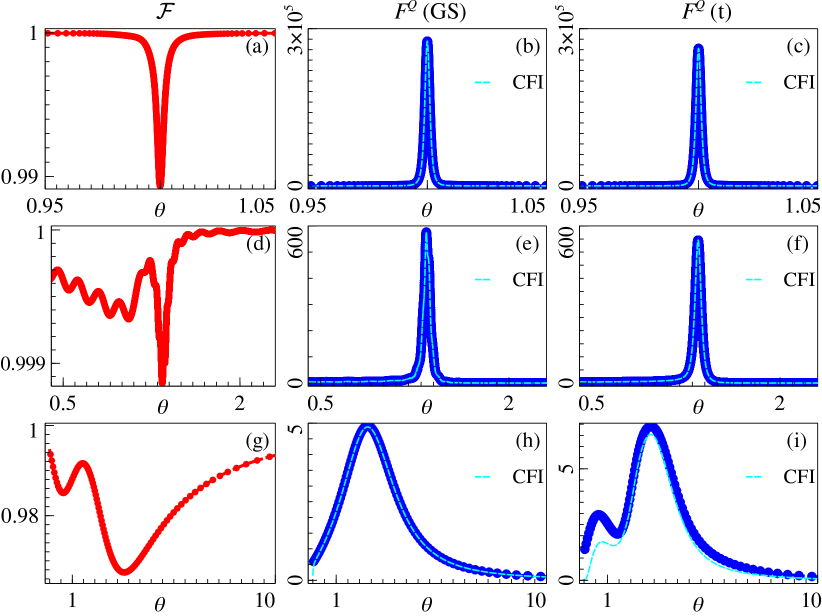
Figure 4: Adiabatic state preparation. (Left coloumn) Fidelity of the adiabatically evolved state with the instantaneous ground state. (Middle coloumn) QFI and CFI of the instantaneous ground state. (Right coloumn) QFI and CFI of the adiabatically evolved state. Top, middle, and bottom rows correspond to Grover, $p$-spin, and biclique spin systems, respectively. In (a), (b), (c) insets zoom in near the critical point. 20-qubit system was used for the Grover model, 30 qubits for the $p$-spin model, and a 5-qubit system with $J{=}1$, $W_{A}{=}4J$ and $W_{B}{=}3.5J$ was used for the biclique system.

To verify the above statement, we numerically prepare the ground state of each of the three models described before using local adiabatic driving Roland and Cerf (2002), which results in $T{\sim}1/\Delta_{c}$. We start with $s{=}0$, i.e. the ground state of $H_{2}$, and then evolve $s$ with time over a long time interval $T$ using a particular schedule $s(t)$. This choice of time-dependent $s(t)$ for local adiabatic driving needs to be fast when the system is far from criticality and slow near the critical point. To get the quantum state at each time one has to solve the Schrodinger equation

$$i\hbar\frac{\partial\ket{\psi(t)}}{\partial t}=H\big{(}s(t)\big{)}\ket{\psi(t)},$$ (15)

with the initial state $\ket{\psi(0)}$ being the ground state of $H_{2}$.

For the Grover model, it can be analytically shown that Roland and Cerf (2002) $s(t)=N\,(\tan^{-1}{\sqrt{N-1}}(2s{-}1)+\tan^{-1}{\sqrt{N{-1}}})\,/\,(2\epsilon\sqrt{N{-}1})$. This results in $T{=}\pi/2\epsilon\Delta_{c}$ where the fidelity between the state of the probe and the instantaneous ground state, namely $\mathcal{F}(t){=}|\bra{\mathrm{GS}(t)}\psi(t)\rangle|^{2}$, is upper bounded as $\mathcal{F}(t){<}(1{-}\epsilon^{2})$. We have numerically verified this in Fig. 4(a), where we plot the fidelity $\mathcal{F}$ versus $\theta$ for a system of size $L{=}20$. As the figure shows, one can achieve a fidelity of $0.99$ at the critical point. Furthermore, we compare the variation of $F^{Q}$ across $\theta_{c}$ for the exact ground state $\ket{\mathrm{GS}(s(t))}$ in Fig. 4(b) and the prepared state $\ket{\psi(s(t))}$ in Fig. 4(c). We observe that for that the small loss of fidelity has very little effect on QFI, which indicates that the exponentially effective quantum sensing at the first order critical point in the Grover model survives under local adiabatic state preparation. For the other two models the schedule $s(t)$ was derived numerically using local adiabatic driving and the total preparation time was expectantly found to be bounded by $1/\Delta_{c}$ (see Appendix A). The corresponding results for the $p$-spin model are shown in Fig. 4(d),(e) and (f), where we observe results similar to the previous case. For the biclique model, as shown in Fig. 4(g), the local adiabatic evolution results in the fidelity going below $0.98$ near the critical point $\theta_{c}$ out of the three systems. Correspondingly, we observe that there is an increase in $F_{Q}$ for the ground state prepared by local adiabatic evolution compared to the exact ground state. It turns out that for small system sizes, the minuscule excitations above the true instantaneous ground state caused by the time evolution results favourably for the QFI.

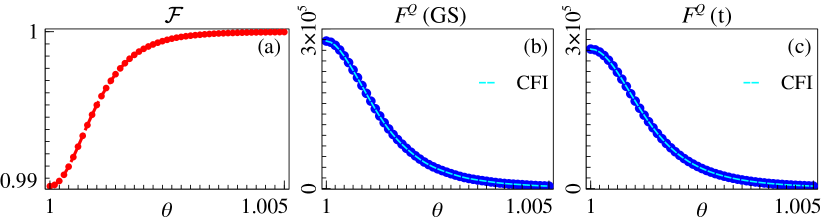
Figure 5: Probe state preparation with unknown parameter. (a) Fidelity of the adiabatically prepared state with actual ground state. (b) QFI and CFI of the ground state. (c) QFI and CFI of the adiabatically prepared state. The results are shown for the Grover model with 20-qubits.

Having established the fact that the critical QFI scales exponentially even after taking the adiabatic preparation time into account, we now give a concrete framework to create the ground state of Eq. (5) for an unknown $\theta$, which is the realistic sensing scenario. We assume that when the sensing apparatus detects $\theta$, its dynamics is governed by Eq. (5), and we know $H_{1}$ and $H_{2}$ (and therefore the critical parameter $\theta_{c}$), but not $\theta$. We then apply a time-dependent control field $s(t)/(1-s(t))$ to the $H_{1}$ component, so that the total Hamiltonian becomes

$$H(\theta,t){=}\frac{s(t)}{(1-s(t))}H_{1}+\theta H_{2}.$$ (16)

The gap closing for this Hamiltonian occurs at $s_{c}{=}\theta/(\theta{+}\theta_{c})$. At $t{=}0$, $s$ is taken to be 0 as before and the initial state is the ground state of $H_{2}$, which can be easily prepared. Using the same adiabatic evolution as before to keep the system in the instantaneous ground state, $s$ is then increased until the value $s{=}1/2$ is reached. At this point, the Hamiltonian given by Eq. (16) takes the form of Eq. (5), and the required probe state is created. The results obtained from applying this method to the Grover model is shown in Fig. 5 for a 20-qubit system near the critical point $\theta_{c}{=}1$. As Fig. 5(a) shows, the fidelity of the prepared state with the actual ground state stays very close to unity. Consequently the QFI and the CFI calculated with the true ground state and the prepared state also match, as shown in Figs. 5 (b) and (c), respectively. Note that here we have taken $\theta{\geq}\theta_{c}$, which makes the gap closing point $s_{C}{\geq}1/2$. This prevents the system from going across the phase transition and the resulting drop in fidelity due to excitations. For a general non-negative $\theta$, we need to employ an additional control field of strength $\theta_{c}$ to the $H_{2}$ component, such that the evolving Hamiltonian becomes $H(\theta,t){=}\frac{s(t)}{(1-s(t))}H_{1}+(\theta+\theta_{c})H_{2}$. This ensures that the system always stays on one side of the critical point and one needs to subtract $\theta_{c}$ from the estimated parameter to obtain the unknown $\theta$.

VI Practical considerations

VI.1 Optimal basis

As shown in Fig. 4, it is possible to determine a set of measurement basis relevant for experimental realization, that seem to be optimal. For the Grover model, $\{\ket{m},\ket{m^{\perp}}\}$ is an optimal basis. For the $p$-spin model, the total magnetization is one optimal basis. For the biclique spin system, the imbalance between the total magnetizations in the two subsystems is given by the operator $\mathcal{I}{=}\sum_{j_{A}=1}^{L_{A}}\sigma^{z}_{j_{A}}-\sum_{j_{B}=1}^{L_{B}}\sigma^{z}_{j_{B}}$. The eigenbasis of this operator serves as an optimal basis.

VI.2 Decoherence

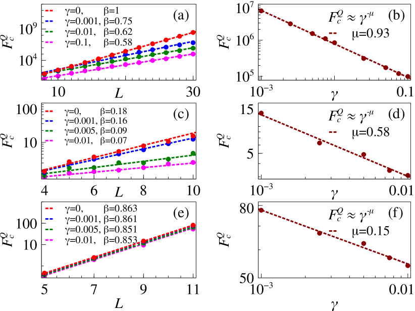
Figure 6: Dephasing dynamics. (Left coloumn) Scaling of critical QFI for various decoherence strength $\gamma$. (Right coloumn) Critical QFI as a function of $\gamma$ at a fixed system size (30, 10, and 11 for Grover, $p$-spin, and biclique systems, respectively). Top, middle, and bottom rows correspond to Grover, $p$-spin, and biclique spin systems ($J{=}1$, $W_{A}{=}4J$, and $W_{B}{=}3.5J$), respectively.

Dephasing is a common source of decoherence in spin system dynamics. To quantify the robustness against dephasing during adiabatic evolution, we employ the master equation formalism for the system density operator $\rho$,

$$\dot{\rho}=-\frac{i}{\hbar}[H,\rho]+\frac{\gamma}{2}\displaystyle\sum_{n}(2c_{n}\rho c_{n}^{{\dagger}}-c_{n}^{{\dagger}}c_{n}\rho-\rho c_{n}^{{\dagger}}c_{n}),$$ (17)

where $\gamma$ is the effective rate of decoherence and $c_{n}$ is the Lindblad operator. For the Grover model, $H{=}H_{\rm Grover}$ and there is only one Lindblad operator $\sigma^{z}$ between the states $\ket{m}$ and $\ket{m^{\perp}}$. Our calculations show that even up to a strong decoherence strength $\gamma{=}0.1$, the signatures of first order phase transition remain intact along with the exponential growth of critical QFI (see Fig. 6(a)). Moreover, $F^{Q}_{c}$ shows an algebraic decay with increasing decoherence strength (see Fig. 6(b) for 30 qubits with exponent ${\approx}0.93$).

For $p$-spin model, $H{=}H_{p\rm-spin}$ and the Lindblad operators are $\sigma^{z}_{j}$. Our calculations show that the exponential growth of $F^{Q}_{c}$ is retained in this case as well, although up to a lower decoherence strength $\gamma{=}0.01J$ (see Fig. 6(c)). For the algebraic decay of $F^{Q}_{c}$ with increasing decoherence strength for 10 qubits, the exponent was ${\approx}0.58$ (see Fig. 6(d)).

For the biclique system with same local Lindblad operators $\sigma^{z}_{j}$, we also found that the exponential growth of $F^{Q}_{c}$ is retained up to a lower decoherence strength $\gamma{=}0.01J$ (see Fig. 6(e)). Up to this strength we see the effect of decoherence is quite weak on the critical QFI values. For the algebraic decay of $F^{Q}_{c}$ with increasing decoherence strength for 11 qubits, the exponent was ${\approx}0.15$ (see Fig. 6(f)).

VI.3 Implementation

Realizing the Grover model requires all-to-all connectivity that can be provided by strongly coupled cavity modes Vaidya et al. (2018); Norcia et al. (2018); Davis et al. (2019); Wang et al. (2015). Such connectivity would also be useful for $p$-spin models. However, another connection between $p$-spin model and ultra-cold bosons bouncing on an oscillating atom mirror was established in Ref. Sacha (2020). The dynamics can be described effectively by a two-mode Bose-Hubbard model when the driving frequency of the mirror is twice of the natural frequency of the bosons falling onto the mirror under gravity Sacha (2015). Mapping between the bosonic operators and spin operators leads to the realization of $p$-spin models with $p{=}2$ for two-body contact interaction. Higher order interactions are speculated to give rise to higher $p$-spin models that are considered in this work.

The biclique system is easy to implement in the D-Wave Pegasus or Zephyr architecture. For example, the Pegasus graph of the D-Wave Advantage system5.4 device hosts 5614-qubits, and one can find the correct embedding of the biclique graph in the setup by using the D-Wave Ocean python package. The architecture already contains $8$-qubit Chimera cells with complete bipartite connectivity Boothby et al. (2020), that can be further coupled by external couplers to achieve a maximum connectivity of $1$ qubit to $15$ qubits. Thus, the maximum system size of the biclique model that can be simulated in D-Wave architecture is $L{=}29$. One has to then initialize the system by setting up the local fields $h_{A}$ and $h_{B}$ in the positions of the real qubits and the couplings $J$. Finally, using the standard quantum annealing protocols to tune $\theta$, one can observe the exponentially enhanced sensitivity near the critical points described in this work.

VI.4 Adaptive estimation strategy

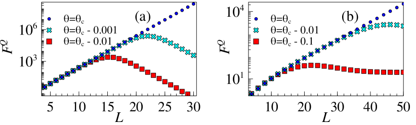
Figure 7: QFI away from criticality. (a) Grover model. (b) $p$-spin model. The maximum size $L$ to sustain exponential sensitivity increases with decreasing distance from criticality. Our adaptive sensing strategy utilizes this feature.

In criticality-based sensing strategies, the quantum advantage is dominantly available in the vicinity of the critical point. Therefore, one needs to tune the probe, e.g. by applying an external control field, to operate near criticality and achieve the best performance. An adaptive strategy is needed to obtain and update prior information iteratively about the unknown parameter Armen et al. (2002); Higgins et al. (2007); Okamoto et al. (2012); Bonato et al. (2016). We now exemplify this adaptive strategy with the Grover model for which analytical results are available. From the expression of QFI in Eq. (13), it is easy to see that for any $\epsilon$ departure from criticality, i.e. for $\theta=\theta_{c}\pm\epsilon$, QFI maximizes for system size

$$L_{\epsilon}=\log_{2}\left(\frac{2(\epsilon-2)\epsilon+4}{\epsilon^{2}}\right),$$ (18)

This gives an optimal length for a given $\epsilon$ up to which the exponential scaling advantage can be obtained and the maximum QFI is $F^{Q}_{\epsilon}=\frac{1}{4(\epsilon-2)^{2}\epsilon^{2}}$. Now the two-step process within each iteration of the adaptive strategy is the following. After the $n$-th step, the estimated parameter value is $\theta_{\rm est}^{(n)}\pm\epsilon^{(n)}$. Then a control field $\theta_{\rm ctl}^{(n)}$ is applied such that $\theta_{\rm est}^{(n)}+\theta_{\rm ctl}^{(n)}=\theta_{c}$. Therefore, the effective prior information about the unknown parameter is $\theta_{\rm eff}^{(n)}=\theta_{c}\pm\epsilon^{(n)}$. For this effective parameter and the given precision $\epsilon^{(n)}$, one can select a probe with optimal size $L_{\epsilon^{(n)}}$, see Eq. (18). With this probe a new set of measurements is performed to update the estimation of the effective parameter to $\theta_{\rm eff}^{(n+1)}$ with a better precision $\epsilon^{(n+1)}$. By deducting the control field, the new prior information for the next step is obtained as $\theta_{\rm est}^{(n+1)}\pm\epsilon^{(n+1)}$. These steps are repeated until the desired precision is achieved. Note that as the precision is improved, the optimal probe size gets larger too which in turn further improves the precision. In Fig. 7(a), the QFI $F^{Q}(\theta)$ is plotted against system size $L$ for different $\epsilon$ values. This shows how the optimal length increases with decreasing $\epsilon$ and the maximum QFI value achievable increases exponentially. The results are qualitatively same for the $p$-spin model, as shown in Fig. 7(b). Although the biclique system shows similar trends, due to the limitation of small system sizes we do not include it in this report.

VII Conclusion

To utilize quantum features for enhancing sensing precision several strategies have been put forward which resulted in sensors based on GHZ-like entangled states, criticality and non-equilibrium dynamics. In most of these methods, the QFI scales algebraically with respect to system size, i.e. $F^{Q}{\sim}L^{\beta}$. Surpassing algebraic advantage and reaching exponential scaling has remained elusive when all the resources, such as the preparation time, are taken into account. Here, we have shown that a class of systems with first order quantum phase transitions with exponential energy gap closing can indeed achieve exponential scaling for the QFI. Remarkably, the exponential scaling nature is preserved even if the state preparation time, through local adiabatic driving, is accounted for. We have illustrated our results by considering three distinct models, namely Grover, $p$-spin, and biclique spin chains, featuring first order phase transition. The results are robust against moderate decoherence and the optimal bases are also experimentally realizable. While criticality-based sensing is inherently local in nature, we have shown, with an adaptive estimation strategy, that it is always possible to harness the exponential scaling for sensing arbitrary parameters to unprecedented precision. Our results can be readily verified on D-wave quantum devices in which the biclique spin system can be easily implemented. This work paves the way for a concrete strategy for precision sensing that has applications in estimating fundamental physical constants which are inherently local sensing problems and require ultra-accurate probes.

Appendix A Preparation time

For the adiabatic state preparation based on the Eq. (15), the condition for the fidelity of the evolved state with the instantaneous ground state to be large, namely, $\mathcal{F}(t){=}|\bra{\mathrm{GS}(t)}\psi(t)\rangle|^{2}<1-\epsilon^{2}$, is

$$\frac{|\braket{\psi_{1}(t)}{\frac{d}{dt}H(t)}{\text{GS}(t)}|}{\Delta(t)^{2}}<\epsilon,$$ (19)

with $\ket{\psi_{1}(t)}$ as the instantaneous first excited state. Transferring the time-dependence on $s(t)$, we can write

$$\frac{dt}{ds}>\frac{|\braket{\psi_{1}(s)}{\frac{d}{ds}H(s)}{\text{GS}(s)}|}{\epsilon\Delta(s)^{2}}.$$ (20)

For the $p$-spin model, we numerically observe that $|\braket{\psi_{1}(s)}{\frac{d}{ds}H(s)}{\text{GS}(s)}|<L$. Therefore we take the preparation time for the ground state at $s$,

$$T(s){=}\int_{0}^{s}\frac{L}{\epsilon\Delta(s)^{2}}ds.$$ (21)

The resulting time was found to scale as ${\sim}e^{0.055L}$ for $p{=}3$ and $\lambda{=}1$, which is advantageous as this exponent as even smaller than that of $1/\Delta_{c}$. Similar results were found for the biclique system as well.

References

- Degen et al. (2017) C. L. Degen, F. Reinhard, and P. Cappellaro, “Quantum sensing,” Reviews of modern physics 89, 035002 (2017).
- Braun et al. (2018) D. Braun, G. Adesso, F. Benatti, R. Floreanini, U. Marzolino, M. W. Mitchell, and S. Pirandola, “Quantum-enhanced measurements without entanglement,” Rev. Mod. Phys. 90, 035006 (2018).
- Ye and Zoller (2024) J. Ye and P. Zoller, “Essay: Quantum sensing with atomic, molecular, and optical platforms for fundamental physics,” Physical Review Letters 132, 190001 (2024).
- Braunstein and Caves (1994) S. L. Braunstein and C. M. Caves, “Statistical distance and the geometry of quantum states,” Phys. Rev. Lett. 72, 3439 (1994).
- Paris (2009) M. G. Paris, “Quantum estimation for quantum technology,” Int. J. Quantum Inf. 07, 125–137 (2009).
- Giovannetti et al. (2004) V. Giovannetti, S. Lloyd, and L. Maccone, “Quantum-enhanced measurements: beating the standard quantum limit,” Science 306, 1330–1336 (2004).
- Giovannetti et al. (2006) V. Giovannetti, S. Lloyd, and L. Maccone, “Quantum metrology,” Physical Review Letters 96, 010401 (2006).
- Giovannetti et al. (2011) V. Giovannetti, S. Lloyd, and L. Maccone, “Advances in quantum metrology,” Nature Photonics 5 (2011), 10.1038/nphoton.2011.35.
- Boixo et al. (2007) S. Boixo, S. T. Flammia, C. M. Caves, and J. M. Geremia, “Generalized limits for single-parameter quantum estimation,” Physical review letters 98, 090401 (2007).
- Raghunandan et al. (2018) M. Raghunandan, J. Wrachtrup, and H. Weimer, “High-density quantum sensing with dissipative first order transitions,” Phys. Rev. Lett. 120, 150501 (2018).
- Mirkhalaf et al. (2020) S. S. Mirkhalaf, E. Witkowska, and L. Lepori, “Supersensitive quantum sensor based on criticality in an antiferromagnetic spinor condensate,” Phys. Rev. A 101, 043609 (2020).
- Yang and Jacob (2019) L.-P. Yang and Z. Jacob, “Engineering first-order quantum phase transitions for weak signal detection,” Journal of Applied Physics 126, 174502 (2019).
- Heugel et al. (2019) T. L. Heugel, M. Biondi, O. Zilberberg, and R. Chitra, “Quantum transducer using a parametric driven-dissipative phase transition,” Physical review letters 123, 173601 (2019).
- Zanardi and Paunković (2006) P. Zanardi and N. Paunković, “Ground state overlap and quantum phase transitions,” Phys. Rev. E 74, 031123 (2006).
- Zanardi et al. (2007) P. Zanardi, H. Quan, X. Wang, and C. Sun, “Mixed-state fidelity and quantum criticality at finite temperature,” Phys. Rev. A 75, 032109 (2007).
- Zanardi et al. (2008) P. Zanardi, M. G. Paris, and L. C. Venuti, “Quantum criticality as a resource for quantum estimation,” Phys. Rev. A 78, 042105 (2008).
- Invernizzi et al. (2008) C. Invernizzi, M. Korbman, L. C. Venuti, and M. G. Paris, “Optimal quantum estimation in spin systems at criticality,” Phys. Rev. A 78, 042106 (2008).
- Gu (2010) S.-J. Gu, “Fidelity approach to quantum phase transitions,” Int. J. Mod. Phys. B 24, 4371–4458 (2010).
- Gammelmark and Mølmer (2011) S. Gammelmark and K. Mølmer, “Phase transitions and heisenberg limited metrology in an ising chain interacting with a single-mode cavity field,” New J. Phys. 13, 053035 (2011).
- Skotiniotis et al. (2015) M. Skotiniotis, P. Sekatski, and W. Dür, “Quantum metrology for the ising hamiltonian with transverse magnetic field,” New J. Phys. 17, 073032 (2015).
- Rams et al. (2018) M. M. Rams, P. Sierant, O. Dutta, P. Horodecki, and J. Zakrzewski, “At the limits of criticality-based quantum metrology: Apparent super-heisenberg scaling revisited,” Phys. Rev. X 8, 021022 (2018).
- Chu et al. (2021) Y. Chu, S. Zhang, B. Yu, and J. Cai, “Dynamic framework for criticality-enhanced quantum sensing,” Phys. Rev. Lett. 126, 010502 (2021).
- Liu et al. (2021) R. Liu, Y. Chen, M. Jiang, X. Yang, Z. Wu, Y. Li, H. Yuan, X. Peng, and J. Du, “Experimental critical quantum metrology with the heisenberg scaling,” npj Quantum Inf. 7, 1–7 (2021).
- Montenegro et al. (2021) V. Montenegro, U. Mishra, and A. Bayat, “Global sensing and its impact for quantum many-body probes with criticality,” Phys. Rev. Lett. 126, 200501 (2021).
- Mishra and Bayat (2021) U. Mishra and A. Bayat, “Driving enhanced quantum sensing in partially accessible many-body systems,” Phys. Rev. Lett. 127, 080504 (2021).
- Mishra and Bayat (2022) U. Mishra and A. Bayat, “Integrable quantum many-body sensors for ac field sensing,” Scientific Reports 12, 14760 (2022).
- Montenegro et al. (2023) V. Montenegro, M. G. Genoni, A. Bayat, and M. G. A. Paris, “Quantum metrology with boundary time crystals,” Communications Physics 6, 304 (2023).
- Iemini et al. (2024) F. Iemini, R. Fazio, and A. Sanpera, “Floquet time crystals as quantum sensors of ac fields,” Phys. Rev. A 109, L050203 (2024).
- Yousefjani et al. (2024a) R. Yousefjani, K. Sacha, and A. Bayat, “Discrete time crystal phase as a resource for quantum enhanced sensing,” arXiv:2405.00328 (2024a).
- Gribben et al. (2024) D. Gribben, A. Sanpera, R. Fazio, J. Marino, and F. Iemini, “Quantum enhancements and entropic constraints to boundary time crystals as sensors of ac fields,” arXiv:2406.06273 (2024).
- He et al. (2023) X. He, R. Yousefjani, and A. Bayat, “Stark localization as a resource for weak-field sensing with super-heisenberg precision,” Phys. Rev. Lett. 131, 010801 (2023).
- Yousefjani et al. (2024b) R. Yousefjani, X. He, A. Carollo, and A. Bayat, “Nonlinearity-enhanced quantum sensing in stark probes,” arXiv:2404.10382 (2024b).
- Yousefjani et al. (2023) R. Yousefjani, X. He, and A. Bayat, “Long-range interacting stark many-body probes with super-heisenberg precision,” Chinese Physics B 32, 100313 (2023).
- Sahoo et al. (2024) A. Sahoo, U. Mishra, and D. Rakshit, “Localization-driven quantum sensing,” Phys. Rev. A 109, L030601 (2024).
- Sarkar et al. (2022) S. Sarkar, C. Mukhopadhyay, A. Alase, and A. Bayat, “Free-fermionic topological quantum sensors,” Phys. Rev. Lett. 129, 090503 (2022).
- Sarkar et al. (2024) S. Sarkar, F. Ciccarello, A. Carollo, and A. Bayat, “Critical non-hermitian topology induced quantum sensing,” New J. Phys. 26, 073010 (2024).
- Montenegro et al. (2024) V. Montenegro, C. Mukhopadhyay, R. Yousefjani, S. Sarkar, U. Mishra, M. G. A. Paris, and A. Bayat, “Review: Quantum metrology and sensing with many-body systems,” arxiv:2408.15323 (2024).
- Ilias et al. (2022) T. Ilias, D. Yang, S. F. Huelga, and M. B. Plenio, “Criticality-enhanced quantum sensing via continuous measurement,” PRX Quantum 3, 010354 (2022).
- Manshouri et al. (2024) H. Manshouri, M. Zarei, M. Abdi, S. Bose, and A. Bayat, “Quantum enhanced sensitivity through many-body bloch oscillations,” arXiv:2406.13921 (2024).
- Roy and Braunstein (2008) S. Roy and S. L. Braunstein, “Exponentially enhanced quantum metrology,” Physical review letters 100, 220501 (2008).
- Wiersig (2014) J. Wiersig, “Enhancing the sensitivity of frequency and energy splitting detection by using exceptional points: Application to microcavity sensors for single-particle detection,” Phys. Rev. Lett. 112, 203901 (2014).
- Chen et al. (2017) W. Chen, Ş. Kaya Özdemir, G. Zhao, J. Wiersig, and L. Yang, “Exceptional points enhance sensing in an optical microcavity,” Nature 548, 192–196 (2017).
- Yu et al. (2020) S. Yu, Y. Meng, J.-S. Tang, X.-Y. Xu, Y.-T. Wang, P. Yin, Z.-J. Ke, W. Liu, Z.-P. Li, Y.-Z. Yang, G. Chen, Y.-J. Han, C.-F. Li, and G.-C. Guo, “Experimental investigation of quantum -enhanced sensor,” Phys. Rev. Lett. 125, 240506 (2020).
- Hodaei et al. (2017) H. Hodaei, A. U. Hassan, S. Wittek, H. Garcia-Gracia, R. El-Ganainy, D. N. Christodoulides, and M. Khajavikhan, “Enhanced sensitivity at higher-order exceptional points,” Nature 548, 187–191 (2017).
- Liu et al. (2016) Z.-P. Liu, J. Zhang, i. m. c. K. Özdemir, B. Peng, H. Jing, X.-Y. Lü, C.-W. Li, L. Yang, F. Nori, and Y.-x. Liu, “Metrology with -symmetric cavities: Enhanced sensitivity near the -phase transition,” Phys. Rev. Lett. 117, 110802 (2016).
- Langbein (2018) W. Langbein, “No exceptional precision of exceptional-point sensors,” Phys. Rev. A 98, 023805 (2018).
- Chen et al. (2019) C. Chen, L. Jin, and R.-B. Liu, “Sensitivity of parameter estimation near the exceptional point of a non-hermitian system,” New Journal of Physics 21, 083002 (2019).
- McDonald and Clerk (2020) A. McDonald and A. A. Clerk, “Exponentially-enhanced quantum sensing with non-hermitian lattice dynamics,” Nature Communications 11, 5382 (2020).
- Budich and Bergholtz (2020) J. C. Budich and E. J. Bergholtz, “Non-hermitian topological sensors,” Phys. Rev. Lett. 125, 180403 (2020).
- Koch and Budich (2022) F. Koch and J. C. Budich, “Quantum non-hermitian topological sensors,” Phys. Rev. Res. 4, 013113 (2022).
- Ding et al. (2023) W. Ding, X. Wang, and S. Chen, “Fundamental sensitivity limits for non-hermitian quantum sensors,” Phys. Rev. Lett. 131, 160801 (2023).
- You et al. (2007) W.-L. You, Y.-W. Li, and S.-J. Gu, “Fidelity, dynamic structure factor, and susceptibility in critical phenomena,” Phys. Rev. E 76, 022101 (2007).
- Roland and Cerf (2002) J. Roland and N. J. Cerf, “Quantum search by local adiabatic evolution,” Phys. Rev. A 65, 042308 (2002).
- Gardner (1985) E. Gardner, “Spin glasses with p-spin interactions,” Nuclear Physics B 257, 747–765 (1985).
- Jörg et al. (2010) T. Jörg, F. Krzakala, J. Kurchan, A. C. Maggs, and J. Pujos, “Energy gaps in quantum first-order mean-field–like transitions: The problems that quantum annealing cannot solve,” EPL 89, 40004 (2010).
- Seki and Nishimori (2012) Y. Seki and H. Nishimori, “Quantum annealing with antiferromagnetic fluctuations,” Phys. Rev. E 85, 051112 (2012).
- Nishimori and Takada (2017) H. Nishimori and K. Takada, “Exponential enhancement of the efficiency of quantum annealing by non-stoquastic hamiltonians,” Frontiers in ICT 4 (2017), 10.3389/fict.2017.00002.
- Karp (1972) R. M. Karp, “Reducibility among combinatorial problems,” (Springer US, Boston, MA, 1972) pp. 85–103.
- Feinstein et al. (2023) N. Feinstein, L. Fry-Bouriaux, S. Bose, and P. A. Warburton, “Effects of xx-catalysts on quantum annealing spectra with perturbative crossings,” arxiv:2203.06779 (2023).
- Ghosh et al. (2024) R. Ghosh, L. A. Nutricati, N. Feinstein, P. A. Warburton, and S. Bose, “Exponential speed-up of quantum annealing via n-local catalysts,” arxiv:2409.13029 (2024).
- McGeoch (2014) C. C. McGeoch, Adiabatic quantum computation and quantum annealing, Synthesis lectures on quantum computing (Springer International Publishing, Cham, 2014).
- Barankov and Polkovnikov (2008) R. Barankov and A. Polkovnikov, “Optimal nonlinear passage through a quantum critical point,” Phys. Rev. Lett. 101, 076801 (2008).
- Rezakhani et al. (2009) A. T. Rezakhani, W.-J. Kuo, A. Hamma, D. A. Lidar, and P. Zanardi, “Quantum adiabatic brachistochrone,” Phys. Rev. Lett. 103, 080502 (2009).
- Grabarits et al. (2024) A. Grabarits, F. Balducci, B. C. Sanders, and A. del Campo, “Non-adiabatic quantum optimization for crossing quantum phase transitions,” arxiv:2407.09596 (2024).
- Vaidya et al. (2018) V. D. Vaidya, Y. Guo, R. M. Kroeze, K. E. Ballantine, A. J. Kollár, J. Keeling, and B. L. Lev, “Tunable-range, photon-mediated atomic interactions in multimode cavity qed,” Phys. Rev. X 8, 011002 (2018).
- Norcia et al. (2018) M. A. Norcia, R. J. Lewis-Swan, J. R. K. Cline, B. Zhu, A. M. Rey, and J. K. Thompson, “Cavity-mediated collective spin-exchange interactions in a strontium superradiant laser,” Science 361, 259–262 (2018).
- Davis et al. (2019) E. J. Davis, G. Bentsen, L. Homeier, T. Li, and M. H. Schleier-Smith, “Photon-mediated spin-exchange dynamics of spin-1 atoms,” Phys. Rev. Lett. 122, 010405 (2019).
- Wang et al. (2015) D.-W. Wang, H. Cai, L. Yuan, S.-Y. Zhu, and R.-B. Liu, “Topological phase transitions in superradiance lattices,” Optica 2, 712–715 (2015).
- Sacha (2020) K. Sacha, Time crystals (Springer, 2020).
- Sacha (2015) K. Sacha, “Modeling spontaneous breaking of time-translation symmetry,” Phys. Rev. A 91, 033617 (2015).
- Boothby et al. (2020) K. Boothby, P. Bunyk, J. Raymond, and A. Roy, “Next-generation topology of d-wave quantum processors,” arXiv:2003.00133 (2020).
- Armen et al. (2002) M. A. Armen, J. K. Au, J. K. Stockton, A. C. Doherty, and H. Mabuchi, “Adaptive homodyne measurement of optical phase,” Phys. Rev. Lett. 89, 133602 (2002).
- Higgins et al. (2007) B. L. Higgins, D. W. Berry, S. D. Bartlett, H. M. Wiseman, and G. J. Pryde, “Entanglement-free heisenberg-limited phase estimation,” Nature 450, 393–396 (2007).
- Okamoto et al. (2012) R. Okamoto, M. Iefuji, S. Oyama, K. Yamagata, H. Imai, A. Fujiwara, and S. Takeuchi, “Experimental demonstration of adaptive quantum state estimation,” Phys. Rev. Lett. 109, 130404 (2012).
- Bonato et al. (2016) C. Bonato, M. S. Blok, H. T. Dinani, D. W. Berry, M. L. Markham, D. J. Twitchen, and R. Hanson, “Optimized quantum sensing with a single electron spin using real-time adaptive measurements,” Nature nanotechnology 11, 247–252 (2016).