Robust microwave cavity control for NV ensemble manipulation

Abstract

Nitrogen-vacancy (NV) center ensembles have the potential to improve a wide range of applications, including nuclear magnetic resonance spectroscopy at the microscale and nanoscale, wide-field magnetometry, and hyperpolarization of nuclear spins via the transfer of optically induced NV polarization to nearby nuclear spin clusters. These NV ensembles can be coherently manipulated with microwave cavities, that deliver strong and homogeneous drivings over large volumes. However, the pulse shaping for microwave cavities presents the added challenge that the external controls and intra-cavity field amplitudes are not identical, leading to adverse effects on the accuracy of operations on the NV ensemble. In this work, we introduce a method based on Gradient Ascent Pulse Engineering (GRAPE) to optimize external controls, resulting in robust pulses within the cavity while minimizing the effects of cavity ringings. The effectiveness of the method is demonstrated by designing both $\pi$ and $\pi/2$ pulses. These optimized controls are then integrated into a PulsePol sequence, where numerical simulations reveal a resilience to detunings five times larger than those tolerated by the sequence constructed using standard controls.

I Introduction

The Nitrogen-vacancy (NV) center [1, 2] is a promising platform for quantum applications owing to its ease of control, which includes optical initialization and readout, microwave coherent manipulation, and long coherence times even at room temperature. NV ensembles are able to detect signals from extremely small volumes, making them promising candidates for spectroscopy at micro- and nanoscale levels [4, 3, 5, 6, 7, 8, 9, 10, 11, 13, 14, 12]. NV ensembles are also being researched for wide-field magnetometry [11, 15, 16, 17], and for dynamical nuclear polarization [18, 19, 20, 22, 21]. In the latter case, the polarization of nearby nuclear spin clusters benefits from the large number of NV centers within the ensemble, as each defect transfers a fraction of polarization to the nuclei.

NV ensembles require strong and uniform drivings to perform accurate unitary operations across the entire ensemble. To achieve such fields, diamonds are often placed within a microwave antenna. This must be engineered to provide the necessary driving strength and spatial homogeneity across the NV ensemble area [25, 24, 26, 23], to enable fast and uniform operations on the defects. In this framework, when the external control on the antenna is kept constant, the amplitude of the intra-cavity field asymptotically approaches a steady state, which is proportional to the control. Thus, when the external control changes, the intra-cavity amplitude approaches a new steady state. This asymptotic behavior is governed by an exponential function, where the rate of accumulation and dissipation of the intra-cavity amplitude is determined by the ringing factor.

For large values of the ringing factor, the cavity reaches its steady state almost instantly, and the shape of the intra-cavity amplitude matches that of the external controls up to a normalization factor (see Eq. (2) and Supplementary Material [27]). In this regime, standard algorithms such as the Gradient Ascent Pulse Engineering (GRAPE) are adequate for pulse shaping optimization [28]. For intermediate values of the ringing factor, where external controls and intra-cavity amplitudes slightly differ, pulse design is still achievable via a piecewise linear approximation [29].

However, for small values of the ringing factor, the cavity’s response time becomes significant, and the intra-cavity amplitudes deviate considerably from the external controls, making the previous approach ineffective. Indeed, a common approach to increase the maximum driving amplitude within the cavity and enable fast operations over NVs is to narrow the ringing factor [24, 23, 30, 31]. Moreover, small ringing factors are a characteristic of resonant cavities radiating a more spatially homogeneous field, making the latter the most interesting case of study for applications with large NV ensembles, and our primary focus.

In this work, we develop a GRAPE-based algorithm to optimize external controls, resulting in robust intra-cavity pulses that perform effectively across an NV ensemble, even in the regime of low ringing factors. We employ our algorithm to generate robust $\pi$ and $\pi/2$ pulses, which are then incorporated into a PulsePol [22] sequence capable of operating over a wide detuning range.

In Section II, we provide the theoretical details of the system under study. Section III outlines the algorithm. In Section IV, we apply the algorithm to enhance the robustness of the PulsePol building blocks against detunings, aiming to improve its inherent robustness. Finally, in Section V, we discuss our findings and explore possibilities for future research.

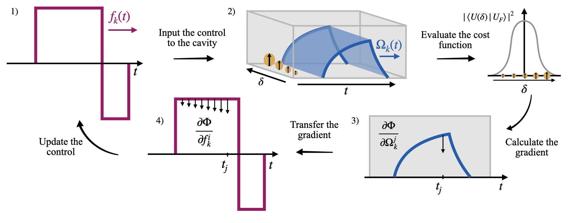
Figure 1: 1) The external control (pink) is inputted to the ODE (2) to obtain $\Omega_{k}(t)$. 2) The internal pulse is applied over an ensemble of spins, i.e. copies of (1) with different values of $\delta$, represented through yellow balls with different sizes. This yields unitaries with varying fidelities $|\braket{U(\delta)}{U_{F}}|^{2}$. 3) The gradient of each fidelity with respect to $\Omega_{k}^{j}$ is computed and summed over the detunings. 4) Subsequently, the gradients are transferred to the external control to update it. Since the ODE makes the value of $\Omega_{k}(t)$ dependent on the external control value at previous times, transferring the gradient corresponding to $\Omega_{k}(t_{j})$ affects to the gradients applied to $f_{k}(t_{i})$ for $t_{i}\leq t_{j}$.

II The system

We consider the Hamiltonian of a spin-$\frac{1}{2}$ Hamiltonian describing a generic NV in an ensemble under the influence of MW drivings [27]:

$$H(t)=\frac{\delta}{2}\sigma_{z}+\sum_{k\in\{x,y\}}\frac{\Omega_{k}(t)}{2}\sigma_{k}.$$ (1)

Here, $\sigma_{x,y,z}$ are Pauli operators, $\delta$ is the detuning of the MW field relative to the NV resonance frequency, which varies from one NV to another in the ensemble; and $\Omega_{x}(t)$ and $\Omega_{y}(t)$ denote the time dependent amplitudes of the applied MW pulses. When the spin is located inside a resonant cavity, the intra-cavity amplitudes ($\Omega_{x}(t)$ and $\Omega_{y}(t)$) are generated by external controls ($f_{x}(t)$ and $f_{y}(t)$) through the following ordinary differential equation (ODE) [34, 32, 27, 33]:

$$\dot{\Omega}_{k}(t)=\gamma\Omega_{\text{max}}f_{k}(t)-\gamma\Omega_{k}(t)\,,\;k\in\{x,y\}.$$ (2)

Here, $f_{k}(t)\in[-1,1]$ represents the normalized amplitude of the external control, $\gamma$ is the ringing factor and $\Omega_{\text{max}}$ denotes the maximum intra-cavity amplitude. Solving Eq. (2) yields:

$$\Omega_{k}(t) =e^{-\gamma(t-t_{0})}\Omega_{k}(t_{0})+$$ (3)

$$+e^{-\gamma(t-t_{0})}\Omega_{\text{max}}\int_{t_{0}}^{t}\gamma f_{k}(t^{\prime})e^{\gamma(t^{\prime}-t_{0})}dt^{\prime},$$

where we consider $\Omega_{k}(t)=0$ at $t=t_{0}$.

To provide intuition for the dynamics of $\Omega_{k}(t)$, consider the cavity’s response to an external control. If the cavity is initially driven by a constant control such that $f_{k}(t)=f_{0}$, the amplitude of $\Omega_{k}(t)$ will asymptotically approach a steady-state value of $f_{0}\Omega_{\text{max}}$, i.e., $\Omega_{k}(t\rightarrow\infty)=f_{0}\Omega_{\text{max}}$. When the external control is turned off (i.e., $f_{k}$ is set to zero), $\Omega_{k}(t)$ decays exponentially over time, a phenomenon known as cavity ringing. Minimizing this ringing is crucial to prevent pulse overlap in sequences with multiple nested pulses.

III The algorithm

Algorithm 1 Chain-GRAPE (our adaptation for cavities).

1: Initial ansatz: $f_{x}$ and $f_{y}$. Vector of detunings: $\vec{\delta}$. Weight of detuning $\delta$: $w_{\delta}$. Ringing correction: $\alpha$.

2: Optimized controls: $f_{x}$ and $f_{y}$.

3:Calculate $\Omega_{k}^{1\times N}$ with $f_{k}^{1\times n_{f}}$.

4:while $1-\Phi\leq$ threshold do

5:     for all $\delta\in\vec{\delta}$ do

6:         Calculate $U_{j}$ from $H(\delta,\Omega_{x}^{j},\Omega_{y}^{j}))$ for all $j\leq N$.

7:         Calculate $\partial\Phi/\partial\Omega_{k}^{j}$.

8:         $D_{k}(j)\leftarrow D_{k}(j)+w_{\delta}\cdot\partial\Phi/\partial\Omega_{k}^{j}$ for all $j\leq N$. (This trains a $\delta$-dependent behavior, providing robustness.)

9:     end for

10:     $D_{k}(N)\leftarrow D_{k}(N)-\alpha\cdot\Omega_{k}^{N}$ (Correction for ringing.)

11:     $G_{k}(i)\leftarrow G_{k}(i)+D_{k}(j)\cdot\partial\Omega_{k}^{j}/\partial f_{k}^{i}$ for all $i\leq\mathtt{ceil}(j/r)$ (Transfer the gradient to the external driving.)

12:     Update $f_{x(y)}$ with the gradients $G_{x(y)}$.

13:end while

14:$\triangleright$ $D_{k}$ and $G_{k}$ account for $\frac{\partial\Phi}{\partial\Omega_{k}}$ and $\frac{\partial\Phi}{\partial f_{k}}$ respectively. They consist of a vector of $N$ and $n_{f}$ elements.

We introduce an algorithm termed Chain-GRAPE, which generates external controls $f_{k}(t)$ that result into time-dependent intra-cavity amplitudes, $\Omega_{k}(t)$. These are capable of implementing arbitrary target unitaries –in the following $U_{F}$– while remaining robust against detunings of several MHz. The discrete nature of the obtained $\Omega_{k}(t)$ results in a unitary of the kind $U(\delta)=U_{N}(\delta)\cdots U_{2}(\delta)\cdot U_{1}(\delta)$, with

$$U_{j}(\delta)=\exp\left\{-2\pi i\left(\frac{\delta}{2}\sigma_{z}+\sum_{k}\Omega_{k}^{j}\frac{\sigma_{k}}{2}\right)dt\right\},$$ (4)

where $dt=\frac{T}{N}$, $T$ refers to the total evolution time and $N$ the number of time steps. In Eq. (4), we take $\Omega_{k}^{j}~{}\equiv~{}\Omega_{k}(jdt)$.

We discretize $\Omega_{k}(t)$ and $f_{k}(t)$ using different time steps, $dt$ and $\Delta t$ respectively, and relate their corresponding number of steps ($N$ and $n_{f}$) by $n_{f}\cdot r=N$, where the ratio $r=\Delta t/dt$. This approach allows us to adapt the algorithm for a small number of time steps ($n_{f}$), which facilitates optimization, while a large $N$ results in an almost continuous curve for $\Omega_{k}(t)$, enabling an accurate simulation of the intra-cavity dynamics. Additionally, the discretization of $f_{k}(t)$ is designed to be compatible with experimental devices that generate controls with a limited sampling rate.

We define the cost function ($\Phi$) [28] for our optimization problem as

$$\Phi=\frac{1}{4}\sum_{\delta}w_{\delta}|\braket{U(\delta)}{U_{F}}|^{2},$$ (5)

where $\braket{A}{B}\equiv\mathrm{tr}(A^{\dagger}B)$ and $w_{\delta}$ is the weight assigned to the bracket $\braket{U(\delta)}{U_{F}}$. The factor of $1/4$ arises from normalizing the trace. By assigning a larger weight to a certain detuning $\delta$, we guide the optimizer to prioritize the matching of $U(\delta)$ to $U_{F}$. In other words, this approach emphasizes the accuracy of the resulting unitary at particular detuning ranges.

The next step is to select an optimizer that successfully yields the controls that maximize the cost function. Among the wide range of optimizers, we focus on gradient-based methods, such as ADAM [35]. This method uses the gradient of $\Phi$ with respect to certain parameters (in our case $f_{k}^{i}~{}\equiv~{}f_{k}(i\Delta t)$) guiding the algorithm toward a maximum of $\Phi$ in parameter space. To calculate the gradient of $\Phi$ with respect to $f_{k}^{i}$ we split it into two parts as follows:

$$\frac{\partial\Phi}{\partial f_{k}^{i}}=\sum_{j=1}^{N}\frac{\partial\Phi}{\partial\Omega_{k}^{j}}\frac{\partial\Omega_{k}^{j}}{\partial f_{k}^{i}}.$$ (6)

The right hand part is computed differentiating Eq. (3):

$$\frac{\partial\Omega_{k}^{j}}{\partial f_{k}^{i}}=e^{-\gamma jdt}\Omega_{\mathrm{max}}\left(e^{\gamma i\Delta t}-e^{\gamma(i-1)\Delta t}\right),$$ (7)

with $i=1,...,i_{c}$ and $i_{c}=\mathtt{ceil}(j/r)$, where $\mathtt{ceil}(x)=\lceil x\rceil=\mathrm{min}\{n\in\mathbb{Z}:x\leq n\}$ [27]. The left-hand term is computed following [28]:

$$\frac{\partial\Phi}{d\Omega_{k}^{j}}= -4\pi idt\cdot$$ (8)

$$\cdot\sum_{\delta}w_{\delta}\text{Re}\bigl{(}\braket{P_{j}(\delta)}{\frac{\sigma_{k}}{2}X_{j}(\delta)}\braket{X_{j}(\delta)}{P_{j}(\delta)}\bigr{)},$$

where $P_{j}(\delta)=U_{j+1}^{\dagger}(\delta)\cdots U_{N}^{\dagger}(\delta)U_{F}$ and $X_{j}(\delta)=U_{j}(\delta)\cdots U_{1}(\delta)$.

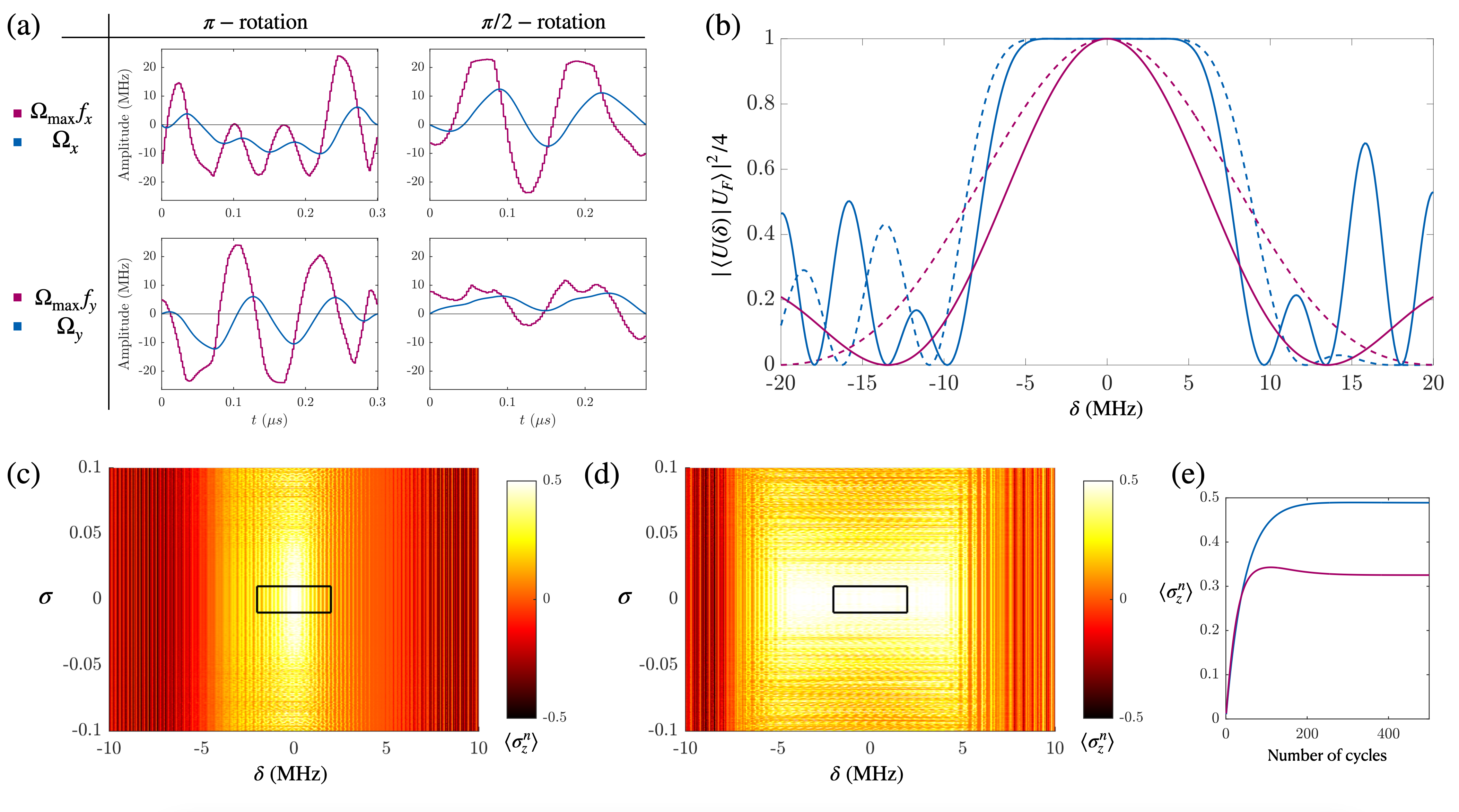
Figure 2: (a) Optimized external (pink) and internal (blue) microwave fields for $\pi$ and $\pi/2$ rotations along the X-axis. The blue curves, representing $\Omega_{k}^{j}$, end with zero amplitude ($\Omega_{k}^{N}\simeq 0$), effectively mitigating cavity ringing effects. (b) Solid lines represent the fidelity $|\braket{U(\delta)}{U_{F}(\theta)}|^{2}$ for $\theta=\pi/2$, while dashed lines correspond to $\theta=\pi$. Remarkably, the blue curves generated with our optimized external controls show resilience to detunings up to 5 MHz. On the contrary, pink curves obtained with the standard controls [27, 34], handle detunings of only up to 1 MHz. Figures (c) and (d) depict the nuclear polarization $\langle\sigma_{z}^{n}\rangle$ (see color-bar) as a function of errors $\delta$ and $\sigma$ after applying the protocol built with the standard pulses and our optimized pulses, respectively. Two PulsePol sequences were applied before reinitializing the NV completing one cycle, and 500 cycles were performed before measuring the nuclear polarization. In (e) we depict the average polarization curve inside the regions marked by the squares in figures (c) and (d). These regions are delimited by the constraints $|\delta|\leq 2\,$MHz and $|\sigma|\leq 0.01$. The curve achieved with our optimized external controls (blue) exceeds those obtained with the standard approach (pink). The values of the parameters used in the simulations are $\gamma=20\,$MHz, $\Omega_{\mathrm{max}}=24\,$MHz, $B_{z}=0.015\,$T, $A_{x}=4\,$kHz and $A_{z}=3.7\,$kHz.

As discussed in Section II, ensuring that the field vanishes within the cavity at the end of the evolution is crucial. Failure to do so would result in undesired dynamics due to the residual amplitude of the controls. To address this, we modify the $j=N$ element of Eq. (8) as

$$\frac{\partial\Phi}{\partial\Omega_{k}^{N}}\rightarrow\frac{\partial\Phi}{\partial\Omega_{k}^{N}}-\alpha\Omega_{k}^{N}.$$ (9)

This adjusts the cost function such that it is maximized when the intra-cavity amplitude at the last step, $\Omega_{k}^{N}$, is small.

This adjustment necessitates choosing an appropriate value for the proportionality constant $\alpha$ to balance the trade-off between maximizing (5) and suppressing ringing, enabling the algorithm to optimize both objectives simultaneously. The complete algorithm is explained in Alg. 1 and Fig. 1.

IV Results

A key application of the proposed algorithm is in designing controls that generate robust pulses for specific pulse sequences, enabling their deployment across large NV ensembles. For instance, in the case of the PulsePol [22] sequence (which is designed for polarization transfer), incorporating our method would further enhance its resilience to detuning errors, thereby extending its applicability to the many NVs escenario.

Now we demonstrate polarization transfer from an NV to a ¹³C nucleus in a wide range of detunings using our method. To achieve gradual polarization transfer, we concatenate polarization cycles by applying the PulsePol sequence twice (note the delivered PulsePol uses our pulses as building blocks) followed by NV reinitialization.

Our algorithm outputs external controls (see Fig. 2 (a) which result in a unitary that approaches

$$U_{F}(\theta)=\exp(-i\theta\sigma_{x}/2),$$ (10)

for $\theta=\pi$ and $\theta=\pi/2$ ($\pi$ and $\pi/2$ pulses respectively), covering detunings up to 5 MHz. These operations are five times more robust than the unitaries generated with the standard controls (see Fig. 2 (b) and Refs. [27, 34] for a description of the standard controls). Since PulsePol requires unitaries along the Y-axis as well (i.e., we also have to target $U_{F}(\theta)=\exp(-i\theta\sigma_{y}/2)$), we need the controls ($f_{x}^{\prime}$ and $f_{y}^{\prime}$) such that $f_{x}^{\prime}=-f_{y}$ and $f_{y}^{\prime}=f_{x}$ [27].

To investigate the added robustness of PulsePol provided by the optimized pulses, we examined the loss of polarization due to detuning $\delta$, as well as to control errors in the Rabi frequency. We have modeled the latter as Gaussian noise, leading to the following modified controls: $\tilde{f}_{k}(t)=f_{k}(t)\cdot[1+\sigma\epsilon(t)]$, where $\epsilon(t)$ stands for random numbers following a unit normal distribution, and $\sigma$ denotes the deviation. Comparing Figs. 2 (c) and 2 (d), we observe that the sequence generated with our optimized pulses exhibits significantly greater resilience to detuning errors compared to the standard approach. We note that detunings are the primary source of error in NV ensembles, while control amplitude deviations are typically around 1$\%$, highlighting the suitability of our method.

In Fig. 2 (e) we plot the average polarization curve, as it is a representative magnitude to compare the speed of the polarization transfer. For that, we first calculate the nuclear polarization after each cycle for each pair values ($\delta$, $\sigma$) enclosed within the black squares in Figs. 2 (c) and 2 (d). The plotted curve is obtained taking the average over all the curves. The results obtained using our pulses show higher polarization, see Fig.2 (e), confirming the enhanced robustness provided by our optimized controls.

V Discussion

We have developed an algorithm to optimize the external controls of a microwave resonant cavity, ensuring that the resulting intra-cavity amplitudes perform the desired unitary operation on NV centers across a broad range of detunings. By optimizing external controls to perform $\pi$ and $\pi/2$ pulses for NV ensembles, we have demonstrated that our algorithm generates robust controls that effectively mitigate ringing effects. Moreover, we have utilized these pulses to construct a PulsePol sequence with enhanced robustness, demonstrating their effectiveness in polarization transfer protocols. This improvement can be extended beyond NV-based methods to other hyperpolarization techniques such as DNP, PHIP, and SABRE [36, 38, 37]. Additionally, the approach can be adapted to systems governed by different transfer functions by recalculating Eq. (7). Lastly, exploring the algorithm’s applicability across various control techniques would be highly valuable. This includes potential integration with mechanical resonators [39], sensing experiments involving ensembles controlled by microwave antennas [26], and superconducting circuits placed within microwave resonant cavities [40].

VI Acknowledgements.–

I.I.Z. acknowledges support from UPV/EHU Ph.D. Grant No. PIF 23/246. C.M.-J. acknowledges the predoctoral MICINN grant PRE2019-088519. J. C. acknowledges the Ramón y Cajal (RYC2018-025197-I) research fellowship. Authors acknowledge the Quench project that has received funding from the European Union’s Horizon Europe – The EU Research and Innovation Programme under grant agreement No 101135742, the Spanish Government via the Nanoscale NMR and complex systems project PID2021-126694NB-C21, and the Basque Government grant IT1470-22.

Supplemental Material:
Robust microwave cavity control for NV ensemble manipulation

I System Hamiltonian

Polarization transfer protocols consist of a polarizing agent and the target nuclei to polarize. We consider one polarizer (the NV center) and a target nucleus (a ¹³C). Acting with a MW driving resonant with the NV leads to the following Hamiltonian:

$$H=(\omega_{n}+A_{z}/2)\sigma_{z}^{n}+\omega\sigma_{z}^{e}/2+\frac{1}{2}\sigma_{z}^{e}\bm{A}\cdot\bm{\sigma}^{n}+\Omega(t)\sigma_{x}^{e}\cos(\omega_{d}t-\phi).$$ (S1)

where $\sigma_{\{x,y,z\}}^{e(n)}$ are the Pauli spin 1/2 operators for the electron (nucleus). Here, we considered that the state $\ket{-1}$ of the NV is not involved in the dynamics. In a rotating frame with respect to $H_{0}=\omega\sigma_{z}^{e}/2$, and invoking the RWA, we get

$$H=(\omega_{n}+A_{z}/2)\sigma_{z}^{n}+\frac{1}{2}\sigma_{z}^{e}\bm{A}\cdot\bm{\sigma}^{n}+\frac{\Omega(t)}{2}\sigma_{\phi}^{e}+\frac{\delta}{2}\sigma_{z}^{e},$$ (S2)

where $\delta=\omega-\omega_{d}$ and $\sigma_{\phi}^{e}=\cos(\phi)\sigma_{x}^{e}+\sin(\phi)\sigma_{y}^{e}$, while we add a time dependency to the phase ($\phi\rightarrow\phi(t)$) which is equivalent of having drivings with X and Y components. Thus, the pulse Hamiltonian reads (note, for simplicity we remove the $e$ superscript)

$$H=\frac{\delta}{2}\sigma_{z}+\frac{\Omega_{x}(t)}{2}\sigma_{x}+\frac{\Omega_{y}(t)}{2}\sigma_{y}.$$ (S3)

which is Eq. (1) of the main text.

II Cavities

Following Refs. [1, 2] we model our microwave cavity as a Fabry-Perot interferometer. Such a device consists of two parallel plates, with an external control $E_{1}(t)e^{-i\omega t}$ and an intra-cavity field $E_{2}(t)e^{-i\omega t}$ which keeps traveling between the plates (see Fig. S1). Considering the frequency of the external control $\omega$ is constant, the external control at $t+\tau$ is added to the already present intra-cavity field:

$$E_{2}(t+\tau)e^{-i\omega(t+\tau)}=\sqrt{T_{1}}E_{1}(t+\tau)e^{-i\omega(t+\tau)}+RE_{2}(t)e^{-i\omega t}.$$ (S4)

Here, $R=\sqrt{R_{1}R_{2}}$ is the survival probability of the intra-cavity field after traveling a round trip, see Fig. S1. Putting the driving on resonance with a frequency of the cavity, the phase accumulated during a round trip is a multiple of $2\pi$, i.e. $\omega\tau=2\pi k$. Then, Eq. (S4) reads

$$E_{2}(t+\tau)=\sqrt{T_{1}}E_{1}(t+\tau)+RE_{2}(t).$$ (S5)

Using the two-point finite difference formula to approximate the derivative gives

$$\frac{E_{2}(t+\tau)-E_{2}(t)}{\tau}=\frac{\sqrt{T_{1}}}{\tau}\left(\dot{E}_{1}(t)\tau+E_{1}(t)\right)+\frac{R-1}{\tau}E_{2}(t).$$ (S6)

We consider that changes in the external control during a round trip are negligible in comparison to its amplitude. More specifically, this is $\dot{E}_{1}(t)\tau\ll E_{1}(t)$, such that

$$\dot{E}_{2}(t)=\frac{\sqrt{T_{1}}}{\tau}E_{1}(t)-\frac{1-R}{\tau}E_{2}(t).$$ (S7)

We define the ringing factor: $\gamma=(1-R)/\tau$. We also redefine $E_{1}$ and $E_{2}$ as

$$E_{1}(t) =E_{\mathrm{max}}\cdot f(t)e^{i\phi_{1}(t)}=E_{\mathrm{max}}\cdot(f_{x}(t)+if_{y}(t)),$$ (S8)

$$E_{2}(t) =\Omega(t)e^{i\phi_{2}(t)}=\Omega_{x}(t)+i\Omega_{y}(t),$$

where $E_{\mathrm{max}}$ is the maximum amplitude of the external control, such that $f(t)$ is normalized

$$|f(t)|^{2}=f_{x}(t)^{2}+f_{y}(t)^{2}\leq 1.$$ (S9)

Examining Eq. (S7) and setting the external control to its maximum value ($E_{\mathrm{max}}$), we observe that $\dot{E}_{2}(t)$ gradually diminishes as $E_{2}$ asymptotically approaches its maximum value

$$E_{2}(t)=\Omega_{\mathrm{max}}=\frac{\sqrt{T_{1}}}{1-R}E_{\mathrm{max}}.$$ (S10)

Now we substitute these definitions in Eq. (S7), and separate the real and imaginary parts which leads to [2]:

$$\dot{\Omega}(t)+\gamma\Omega(t) =\gamma\Omega_{\mathrm{max}}f(t)\cos(\phi_{2}(t)-\phi_{1}(t)),$$ (S11)

$$\dot{\phi}_{2} =-\gamma\Omega_{\mathrm{max}}\frac{f(t)}{\Omega(t)}\sin(\phi_{2}(t)-\phi_{1}(t)).$$

To avoid the singularity when $\Omega(t)=0$, we obtain the equivalent system of equations for the real and imaginary parts of the fields, instead of the amplitude and phase:

$$\dot{\Omega}_{k}(t)+\gamma\Omega_{k}(t)=\gamma\Omega_{\mathrm{max}}f_{k}(t),$$ (S12)

with $k\in\{x,y\}$. These equations are linear and analytically solvable for piecewise constant $f_{x}(t)$ and $f_{y}(t)$.

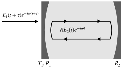
Figure S1: Diagram of fields inside and outside the cavity modeled as a Fabry-Perot interferometer. At every round trip, the external driving will sum to the field inside the cavity.

II.1 Analytical solution of the ODE

The analytical solution of the system in Eq. (S12) can be obtained treating each of them independently and using an integrator factor $\mu(x,y)$ that transforms the equation $P(x,y)dx+Q(x,y)dy=0$ in the exact equation

$$\mu(x,y)[P(x,y)dx+Q(x,y)dy]=0,$$ (S13)

where $\displaystyle\frac{\partial\mu P}{\partial y}=\frac{\partial\mu Q}{\partial x}$. When the structure of the ODE follows

$$y^{\prime}+A(x)y=B(x)\quad\Longrightarrow\quad\left\{\begin{aligned} P&=(A(x)y-B(x))\\ Q&=1\end{aligned}\right.,$$ (S14)

one can prove that the integration factor has the form

$$\mu(x)=e^{\int Adx}.$$ (S15)

And the equation becomes

$$e^{\int Adx}y^{\prime}+e^{\int Adx}A(x)y=e^{\int Adx}B(x)\;\rightarrow\;\frac{d}{dx}\left(e^{\int Adx}y\right)=Be^{\int Adx},$$ (S16)

which results in

$$y=e^{-\int Adx}\left(C+\int Be^{\int Adx}dx^{\prime}\right).$$ (S17)

By substituting $A=\gamma$ and $B=\gamma\Omega_{\text{max}}f_{k}(t)$ we get

$$\Omega_{k}(t)=e^{-\gamma(t-t_{0})}\Omega_{k}(t_{0})+e^{-\gamma(t-t_{0})}\Omega_{\text{max}}\int_{t_{0}}^{t}\gamma f_{k}(t^{\prime})e^{\gamma(t^{\prime}-t_{0})}dt^{\prime},$$ (S18)

which is Eq. (3) in the main text.

II.2 Ringing

For large values of $\gamma$, $\Omega_{k}(t)$ approaches $\Omega_{\mathrm{max}}f_{k}(t)$. To analyze that effect we calculate how long it takes to the intra-cavity amplitude to reach $\Omega_{\mathrm{max}}/2$ starting from 0:

$$\Omega_{\mathrm{max}}/2=e^{-\gamma t}\Omega_{\mathrm{max}}\left(e^{\gamma t}-1\right)=\Omega_{\mathrm{max}}\left(1-e^{-\gamma t}\right)\Longrightarrow 1/2=e^{-\gamma t}\Longrightarrow t=\frac{1}{\gamma}\ln 2.$$ (S19)

If each step of $f_{k}$ is much longer than $t=\frac{1}{\gamma}\ln 2$, $\Omega_{k}(t)$ is similar to $f_{k}(t)$, and we can consider intra-cavity amplitudes as square fuctions.

For cavities with large quality factor, i.e. small $\gamma$, when the driving is switched off the intra-cavity amplitude decays exponentially, which further evolves the NVs. This effect is called cavity ringing, and in [3] an analytical solution is proposed (see Fig. S2), so that the intra-cavity amplitude vanishes at the end of the pulse.

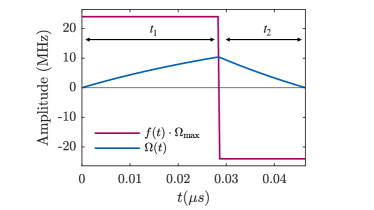
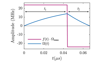
Figure S2: The plot on the left (right) depicts the fastest (and standard) way of applying a $\pi/2$ ($\pi$) pulse on a system inside a cavity. The external control is plotted in pink, and the intra-cavity amplitude in blue. The solution consists of applying an external control with duration $t_{1}$, followed by a negative, i.e. $\pi$-dephased, control with duration $t_{2}$. Here we set $\Omega_{\mathrm{max}}=24\,$MHz and $\gamma=20\,$MHz.

III Derivation of the gradient

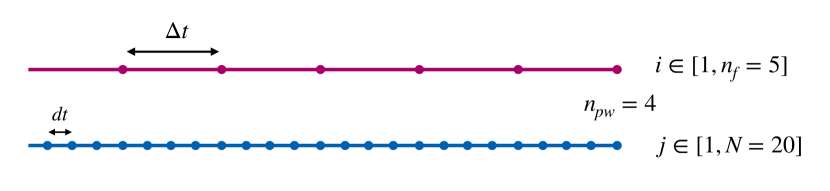
Figure S3: Diagram of the discretization of the external controls (pink) and intra-cavity amplitudes (blue).

We emphasize that the number of steps of $\Omega(t)$, denoted as $N$, has to be large, whereas the one of $f(t)$ ($n_{f}$) should be kept small in order to have fewer parameters to optimize. Thus, we define $r=N/n_{f}$ to be an integer number (see Fig. S3). Using the following notation

$$\lfloor x\rfloor =\mathtt{floor}(x)=\max\{n\in\mathbb{Z}:n\leq x\}$$ (S20)

$$\lceil x\rceil =\mathtt{ceil}(x)=\min\{n\in\mathbb{Z}:x\leq n\},$$

we rewrite Eq. (S18) as a sum of integrals (considering $f_{k}^{i}=f_{k}(i\Delta t)$ constant) over the completed $\Delta t$ steps, and an extra term that appears when the last step is uncompleted (i.e. $t<i_{c}\Delta t$):

$$\Omega_{k}(t)=e^{-\gamma t}\Omega_{\mathrm{max}}\gamma\left(\sum_{i=1}^{i_{f}}\int_{(i-1)\Delta t}^{i\Delta t}f_{k}^{i}e^{\gamma t^{\prime}}dt^{\prime}+\int_{i_{f}\Delta t}^{jdt}f_{k}^{i_{c}}e^{\gamma t^{\prime}}dt^{\prime}\right),$$ (S21)

where $i_{f}=\lfloor\frac{t}{\Delta t}\rfloor$ and $i_{c}=\lceil\frac{t}{\Delta t}\rceil$. And solving the integrals,

$$\Omega_{k}(t)=e^{-\gamma t}\Omega_{\mathrm{max}}\left(\sum_{i=1}^{i_{f}}f_{k}^{i}\left(e^{\gamma i\Delta t}-e^{\gamma(i-1)\Delta t}\right)+f_{k}^{i_{c}}\left(e^{\gamma t}-e^{\gamma i_{f}\Delta t}\right)\right).$$ (S22)

Substituting that $t=jdt$ for $j=1,...,N$

$$\Omega_{k}^{j}=e^{-\gamma jdt}\Omega_{\mathrm{max}}\sum_{i=1}^{i_{f}}f_{k}^{i}\left(e^{\gamma i\Delta t}-e^{\gamma(i-1)\Delta t}\right)+f_{k}^{i_{c}}\left(e^{\gamma jdt}-e^{\gamma i_{f}\Delta t}\right).$$ (S23)

We calculate $d\Omega_{k}^{j}/df_{k}^{i}$ differentiating Eq. (S23), and get a conditional expression on $i$ and $j$, since we can redefine $i_{f}=\lfloor j/r\rfloor$ and $i_{c}=\lceil j/r\rceil$, such that they depend on $j$

$$\frac{\partial\Omega_{k}^{j}}{\partial f_{k}^{i}}=\left\{\begin{aligned} &e^{-\gamma jdt}\Omega_{\mathrm{max}}\left(e^{\gamma i\Delta t}-e^{\gamma(i-1)\Delta t}\right),\;i\leq i_{f}.\\ &e^{-\gamma jdt}\Omega_{\mathrm{max}}\left(e^{\gamma jdt}-e^{\gamma i_{f}\Delta t}\right),\;i_{f}<i=i_{c}.\\ &0,\;\text{otherwise}.\end{aligned}\right.$$ (S24)

For the sake of simplicity, and after numerical validation, we approximate the gradient as

$$\frac{\partial\Omega_{k}^{j}}{\partial f_{k}^{i}}=e^{-\gamma jdt}\Omega_{\mathrm{max}}\left(e^{\gamma i\Delta t}-e^{\gamma(i-1)\Delta t}\right)$$ (S25)

for every $j=1,...,N$ and $i=1,...,i_{c}$.

IV Energy constrained pulses

From Eq. (S10) one could think that the maximum intra-cavity amplitude achievable can grow indefinitely, as we increase the amplitude of the external control $E_{\mathrm{max}}$. However, when increasing the input power the antenna overheats [4] and the performance worsens, making us fix an affordable value of $\Omega_{\mathrm{max}}$. To ensure the algorithm provides pulses that obey the constraint of (S9), we verify that $f(t)$ remains within the unit circle for all $t$. In the case it falls outside, we project it onto the boundary (the circumference of radius one) keeping the same angle $\theta=\tan^{-1}\left(\frac{f_{y}(t)}{f_{x}(t)}\right)$. We repeat this process every time the optimizer updates the external control.

V Pulses along other axes

To build the PulsePol sequence, $\pi$ and $\pi/2$ pulses are also required along the Y-axis. While we have optimized the controls for pulses along the X-axis, the controls for the Y-axis pulses can be obtained by applying a specific transformation to the original set. In Fig. S4 we rotate the axes to make the Y-axis coincide with the pink arrow. Now, the arrow $f_{x}$ coincides with the Y-axis, and $f_{y}$ with the -X-axis. So, the transformation is $f_{x}^{\prime}=-f_{y}$ and $f_{y}^{\prime}=f_{x}$; equivalent to $f^{\prime}=e^{i\pi/2}fe^{i\phi_{1}}=-f_{y}+if_{x}$, see (S8).

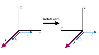
Figure S4: Diagram of the transformation. The pink arrow indicates along what axis happens the rotation. The blue arrows are the controls corresponding to that rotation.

References

- [1] M. W. Doherty, N. B. Manson, P. Delaney, F. Jelezko, J. Wrachtrup, and L. C. L. Hollenberg, The nitrogen-vacancy colour centre in diamond, Phys. Rep. 528, 1 (2013).
- [2] D. D. Awschalom, R. Hanson, J. Wrachtrup, and B. B. Zhou, Quantum technologies with optically interfaced solid-state spins , Nat. Photon. 12, 516 (2018).
- [3] N. Arunkumar, D. B. Bucher, M. J. Turner, P. TomHon, D. Glenn, S. Lehmkuhl, M. D. Lukin, H. Park, M. S. Rosen, T. Theis, R. L. Walsworth, Micron-scale NV NMR spectroscopy with signal amplification by reversible exchange, PRX Quantum 2, 010305 (2021).
- [4] D. R. Glenn, D. B. Bucher, J. Lee, M. D. Lukin, H. Park and R. L. Walsworth, High-resolution magnetic resonance spectroscopy using a solid-state spin sensor, Nature 555, 351 (2018).
- [5] D. B. Bucher, D. R. Glenn, H. Park, M. D. Lukin, and R. L. Walsworth, Hyperpolarization-enhanced NMR spectroscopy with femtomole sensitivity using quantum defects in diamond, Phys. Rev. X 10, 021053 (2020).
- [6] R. D. Allert, K. D. Briegel, and D. B. Bucher, Advances in nano- and microscale NMR spectroscopy using diamond quantum sensors, Chem. Commun. 58, 8165 (2022).
- [7] H. J. Mamin, M. Kim, M. H. Sherwood, C. T. Rettner, K. Ohno, D. D. Awschalom, and D. Rugar, Nanoscale nuclear magnetic resonance with a nitrogen-vacancy spin sensor, Science 339, 557 (2013).
- [8] T. Staudacher, F. Shi, S. Pezzagna, J. Meijer, J. Du, C. A. Meriles, F. Reinhard, and J. Wrachtrup, Nuclear magnetic resonance spectroscopy on a (5-nanometer)3 sample volume, Science 339, 561 (2013).
- [9] T. F. Segawa and R. Igarashi, Nanoscale quantum sensing with Nitrogen-Vacancy centers in nanodiamonds – A magnetic resonance perspective, Prog. Nucl. Magn. Reson. Spectrosc. 134, 20 (2023).
- [10] R. Schirhagl, K. Chang, M. Loretz, and C. L. Degen, Nitrogen-Vacancy centers in diamond: nanoscale sensors for physics and biology, Annu. Rev. Phys. Chem. 65, 83 (2014).
- [11] S. Hong, M. S. Grinolds, L. M. Pham, D. Le Sage, L. Luan, R. L. Walsworth, and A. Yacoby, Nanoscale magnetometry with NV centers in diamond, MRS Bull. 38, 155 (2013).
- [12] C. Munuera-Javaloy, A. Tobalina, and J. Casanova, High-resolution NMR spectroscopy at large fields with nitrogen vacancy centers, Phys. Rev. Lett. 130, 133603 (2023).
- [13] P. Alsina-Bolívar, A. Biteri-Uribarren, C. Munuera-Javaloy, and J. Casanova, J-coupling NMR spectroscopy with nitrogen vacancy centers at high fields, Phys. Rev. Research 6, 043017 (2024).
- [14] C. Munuera-Javaloy, A. Tobalina, J. Casanova, High-field microscale NMR spectroscopy with NV centers in dipolarly-coupled samples, arXiv:2405.12857.
- [15] D. Le Sage, K. Arai, D. R. Glenn, S. J. DeVience, L. M. Pham, L. Rahn-Lee, M. D. Lukin, A. Yacoby, A. Komeili and R. L. Walsworth, Optical magnetic imaging of living cells, Nature 496, 486 (2013).
- [16] S. Sengottuvel, M. Mrózek, M. Sawczak, M. J. Glowacki, M. Ficek, W. Gawlik, and A. M. Wojciechowski, Wide-field magnetometry using nitrogen-vacancy color centers with randomly oriented micro-diamonds, Sci. Rep. 12, 17997 (2022).
- [17] Z. Guo, Y. Huang, M. Cai, C. Li, M. Shen, M. Wang, P. Yu, Y. Wang, F. Shi, P. Wang, and J. Du, Wide-field Fourier magnetic imaging with electron spins in diamond, npj Quantum Inf. 10, 24 (2024).
- [18] D. Pagliero, K. R. K. Rao, P. R. Zangara, S. Dhomkar, H. H. Wong, A. Abril, N. Aslam, A. Parker, J. King, C. E. Avalos, A. Ajoy, J. Wrachtrup, A. Pines, and C. A. Meriles, Multispin-assisted optical pumping of bulk 13C nuclear spin polarization in diamond, Phys. Rev. B 97, 024422 (2018).
- [19] A. Ajoy, K. Liu, R. Nazaryan, X. Lv, P. R. Zangara, B. Safvati, G. Wang, D. Arnold, G. Li, A. Lin, P. Raghavan, E. Druga, S. Dhomkar, D. Pagliero, J. A. Reimer, D. Suter, C. A. Meriles, and A. Pines, Orientation-independent room temperature optical 13C hyperpolarization in powdered diamond, Sci. Adv. 4, eaar5492 (2018).
- [20] J.-P. Tetienne, L. T. Hall, A. J. Healey, G. A. L. White, M.-A. Sani, F. Separovic, and L. C. L. Hollenberg, Prospects for nuclear spin hyperpolarization of molecular samples using nitrogen-vacancy centers in diamond, Phys. Rev. B 103, 014434 (2021).
- [21] Q. Chen, I. Schwarz, F. Jelezko, A. Retzker, and M. B. Plenio, Optical hyperpolarization of 13C nuclear spins in nanodiamond ensembles, Phys. Rev. B 92, 184420 (2015).
- [22] I. Schwartz , J. Scheuer, B. Tratzmiller, S. Müller, Q. Chen, Ish Dhand, Z.-Y. Wang, C. Müller, B. Naydenov, F. Jelezko, and M. B. Plenio, Robust optical polarization of nuclear spin baths using Hamiltonian engineering of nitrogen-vacancy center quantum dynamics, Sci. Adv. 4, eaat8978 (2018).
- [23] O. R. Opaluch, N. Oshnik, R. Nelz, and E. Neu, Optimized planar microwave antenna for nitrogen vacancy center based sensing applications, Nanomaterials 11, 2108 (2021).
- [24] R. Pellicer-Guridi, K. Custers, J. Solozabal-Aldalur, A. Brodolin, J. T. Francis, M. Varga, J. Casanova, M. M. Paulides, and G. Molina-Gerriza, Versatile quadrature antenna for precise control of large electron spin ensembles in diamond, arXiv:2401.11986.
- [25] D. Yudilevich, A. Salhov, I. Schaefer, K. Herb, A. Retzker, and A. Finkler, Coherent manipulation of nuclear spins in the strong driving regime, New J. Phys. 25 113042 (2023).
- [26] N. Arunkumar, K. S. Olsson, J. T. Oon, C. A. Hart, D. B. Bucher, D. R. Glenn, M. D. Lukin, H. Park, D. Ham, and R. L. Walsworth, Quantum logic enhanced sensing in solid-state spin ensembles, Phys. Rev. Lett. 131, 100801 (2023).
- [27] See Supplementary Material for detailed information.
- [28] N. Khaneja, T. Reiss, C. Kehlet, T. Schulte-Herbrügen, and S. J. Glaser, Optimal control of coupled spin dynamics: design of NMR pulse sequences by gradient ascent algorithms, J. Magn. Reson. 172, 296 (2005).
- [29] U. Rasulov, A. Acharya, M. Carravetta, G. Mathies, I. Kuprov, Simulation and design of shaped pulses beyond the piecewise-constant approximation, J. Magn. Reson. 353, 107478 (2023).
- [30] A. E. Siegman, Lasers, Optica (1986).
- [31] D. M. Pozar, Microwave Engineering, 4th edition, Wiley (2012).
- [32] J. C. Bienfang, R. F. Teehan, and C. A. Denman, Phase noise transfer in resonant optical cavities, Rev. Sci. Instrum. 72, 3208 (2001).
- [33] M. J. Lawrence, B. Willke, M. E. Husman, E. K. Gustafson, and R. L. Byer, Dynamic response of a Fabry-Perot interferometer, J. Opt. Soc. Am. B 16, 523 (1999).
- [34] B. Tratzmiller, Pulsed control methods with applications to nuclear hyperpolarization and nanoscale NMR, OPARU (2021).
- [35] D. P. Kingma, J. Ba, Adam: A method for stochastic optimization, arXiv: 1412.6980.
- [36] K. V. Kovtunov, E. V. Pokochueva, O. G. Salnikov, S. F. Cousin, D. Kurzbach, B. Vuichoud, S. Jannin, E. Y. Chekmenev, B. M. Goodson, D. A. Barskiy, and I. V. Koptyug, Hyperpolarized NMR Spectroscopy: d-DNP, PHIP, and SABRE Techniques, Chem. Asian J. 13, 1857 (2018).
- [37] M. C. Korzeczek, L. Dagys, C. Müller, B. Tratzmiller, A. Salhov, T. Eichhorn, J. Scheuer, S. Knecht, M. B. Plenio, and I. Schwartz, Towards a unified picture of polarization transfer — pulsed DNP and chemically equivalent PHIP, J. Magn. Reson. 362, 107671 (2024).
- [38] J.-B. Hövener, A. N. Pravdivtsev, B. Kidd, C. R. Bowers, S. Glöggler, K. V. Kovtunov, M. Plaumann, R. Katz-Brull, K. Buckenmaier, A. Jerschow, F. Reineri, T. Theis, R. V. Shchepin, S. Wagner, P. Bhattacharya, N. M. Zacharias, and E. Y. Chekmenev, Parahydrogen-Based Hyperpolarization for Biomedicine, Angew. Chem. Int. Ed. 57, 11140 (2018).
- [39] E. R. MacQuarrie, T. A. Gosavi, A. M. Moehle, N. R. Jungwirth, S. A. Bhave, and G. D. Fuchs, Coherent control of a nitrogen-vacancy center spin ensemble with a diamond mechanical resonator, Optica 2, 233 (2015).
- [40] M. Naghiloo, Introduction to experimental quantum measurement with superconducting qubits, arXiv:1904.09291.

References

- [1] M. J. Lawrence, B. Willke, M. E. Husman, E. K. Gustafson, and R. L. Byer, Dynamic response of a Fabry-Perot interferometer, J. Opt. Soc. Am. B: Opt. Phys. 16(4), 523-532 (1999).
- [2] J. C. Bienfang, R. F. Teehan, and C. A. Denman, Phase noise transfer in resonant optical cavities, Rev. Sci. Instrum. 72, 3208–3214 (2001).
- [3] B. Tratzmiller, Pulsed control methods with applications to nuclear hyperpolarization and nanoscale NMR, OPARU (2021).
- [4] R. Pellicer-Guridi, K. Custers, J. Solozabal-Aldalur, A. Brodolin, J. T. Francis, M. Varga, J. Casanova, M. M. Paulides, and G. Molina-Gerriza, Versatile quadrature antenna for precise control of large electron spin ensembles in diamond, arXiv:2401.11986.