Principled Bayesian Optimisation
in Collaboration with Human Experts

Abstract

Bayesian optimisation for real-world problems is often performed interactively with human experts, and integrating their domain knowledge is key to accelerate the optimisation process. We consider a setup where experts provide advice on the next query point through binary accept/reject recommendations (labels). Experts’ labels are often costly, requiring efficient use of their efforts, and can at the same time be unreliable, requiring careful adjustment of the degree to which any expert is trusted. We introduce the first principled approach that provides two key guarantees. (1) Handover guarantee: similar to a no-regret property, we establish a sublinear bound on the cumulative number of experts’ binary labels. Initially, multiple labels per query are needed, but the number of expert labels required asymptotically converges to zero, saving both expert effort and computation time. (2) No-harm guarantee with data-driven trust level adjustment: our adaptive trust level ensures that the convergence rate will not be worse than the one without using advice, even if the advice from experts is adversarial. Unlike existing methods that employ a user-defined function that hand-tunes the trust level adjustment, our approach enables data-driven adjustments. Real-world applications empirically demonstrate that our method not only outperforms existing baselines, but also maintains robustness despite varying labelling accuracy, in tasks of battery design with human experts.

1 Introduction

Bayesian optimisation (BO) [59, 64, 33] is a successful approach to black-box optimiation that has been applied across a wide array of applications. BO is often praised for ‘taking the human out of the loop’ [79] by automating laborious optimisation processes, such as hyperparameter optimisation [29, 102] and neural architecture search [73, 98], thus relieving human users from these tasks. Nonetheless, a growing trend involves the opposite direction, which brings humans back into the loop and leverages human expertise as an adviser to the optimiser [7]. This human-in-the-loop approach is particularly relevant to scientific and explorative tasks, such as materials discovery [24, 2] and product design [47, 43, 7]. Experts have accumulated domain knowledge and should be helpful in accelerating the optimisation process, yet their experience and knowledge are often qualitative—they can struggle to express their knowledge in a functional form or to pinpoint the best candidates as an absolute quantity [46]. At the forefront of science, experts are also in the middle of trial and error; demanding well-defined and error-free inputs can limit the applicable range of BO. As such, a human-AI collaborative setting in BO has emerged, driven by practical demands, and has been gaining popularity in the literature [11, 42, 38, 49, 24, 7, 69, 12, 41].

A prevalent issue in this domain is the lack of both shared assumptions and theoretical guarantees, making fair comparisons challenging. Our community has yet to reach a consensus on acceptable assumptions, particularly in the following areas. (a) The level of effectiveness of experts’ knowledge: assuming near oracle-like knowledge, e.g. in [11, 38, 12], collaborative settings can significantly surpass vanilla BO. However, if experts are entirely erroneous (yet confident)—which can happen [42, 49, 24, 7]—overreliance on experts’ input cannot guarantee the global optimum convergence. (b) Human interaction method: ideally, humans prefer minimising interaction with machines for convenience. Minimising interaction leads to maximising the information at each query to human, which often ends up requesting error-free and quantitative information for humans [81, 11, 42, 41]. However, accurate knowledge elicitation remains a long-standing quest [78, 67, 57]. Inversely, when we assume human belief is also a black-box function and require the elicitation of the belief function through statistical modelling, e.g. [72, 34, 7], we will demand excessive queries of the experts.

Contributions. The contributions of this paper are summarised below:

1. Handover guarantee: we model the expert’s role as cognitively simple and qualitative—the expert serves as a black-box classifier, providing binary labels on the desirability of the next query location. Similar to the no-regret property, we establish a sublinear bound on the cumulative number of binary labels needed. Initially, multiple labels per query are needed, but the frequency of querying binary labels asymptotically converges to zero, thus saving both expert effort and computation time.

2. No-harm guarantee: we show that the convergence rate of our expert-advised algorithm will not be worse than that of vanilla BO (i.e. without expert advice), even if the advice from experts is adversarial. Our convergence is achieved through data-driven trust level adjustments, and is unlike existing methods that rely on hand-tuned user-defined functions.

3. Real-world contribution: empirically, our algorithm provides both fast convergence and resilience against erroneous inputs. It outperformed existing methods in both popular synthetic, and new real-world, tasks in designing lithium-ion batteries.

2 Problem Statement

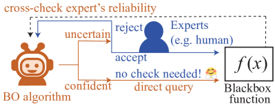
Figure 1: BO-expert collaboration framework: The algorithm (red) decides if an expert’s (blue) label is necessary. If rejected, it generates a different candidate; otherwise, it directly queries.

We address the black-box optimization problem,

$$x^{\star}\in\arg\min_{x\in\mathcal{X}}\;f(x)\;,$$ (1)

while collaborating with an expert, where $\mathcal{X}\subset\mathbb{R}^{d}$ and $d$ is the dimension.

Expert labelling model. We model an expert as a binary labeller (see Fig. 1). An expert labels a point $x\in\mathcal{X}$ as either ‘accept’ or ‘reject’. An ‘accept’ label indicates that the point is worth sampling, while ‘reject’ label indicates it is not. These labels are binary, with $0$ for ‘accept’ and $1$ for ‘reject’. In practice, the labelling process can be noisy, since humans may find some points hard to classify. Non-expert or incorrect belief may label the optimum $x^{\star}$ ‘reject’. The distribution of the labels is determined by the expert’s prior belief about the black-box function $f$, and we model the expert’s belief through another unknown black-box function $g$.

Assumption 2.1.

The notation $x\succ_{g}0$ denotes the event where $x$ is labelled as ‘reject’, based on the expert’s belief function $g$. Additionally, the random indicator $\mathbf{1}_{x\succ_{g}0}\in\{0,1\}$ takes value $1$ if $x\succ_{g}0$ and $0$ otherwise. The probability distribution of $\mathbf{1}_{x\succ_{g}0}\in\{0,1\}$ follows the Bernoulli distribution with $\mathbb{P}(\mathbf{1}_{x\succ_{g}0}=1)=p_{x\succ_{g}0}=S(g(x))$, where $S(u)=\nicefrac{{1}}{{(1+e^{-u})}}$ is the sigmoid function.

Example 2.2.

Let us define an example ‘synthetic’ expert’s labelling response as $p_{x\succ_{g}0}=S(a\rho(f(x)))$, where $a$ is the accuracy coefficient and $\rho$ is the linear scaling function from bound $[\min_{x\in\mathcal{X}}f(x),\max_{x\in\mathcal{X}}f(x)]$ to $[-3,3]$. When $a=1$, $\rho(f(x^{*}))=-3,S(-3)\approx 0.05$, resulting in a Bernoulli distribution that yields an acceptance label of 0 with a 95% chance at the global minimum $x^{*}$. In this case, the sharpness of the belief $p_{x\succ_{g}0}$ is influenced by both the shape of $f(x)$ and $a$; if $f(x)$ is peaky or $a\gg 1$, the expert can nearly pinpoint $x^{*}$.

However, in reality, the expert does not know the exact true $f$ and therefore, we consider $g$ to be a ‘subjective’ belief function representing $f$. This differs from a typical surrogate model $\hat{f}$ of $f$, which infers an ‘objective’ belief function from oracle queries. If $g$ has better predictive ability than the surrogate model $\hat{f}$, exploiting $g$ can accelerate convergence; otherwise it may decelerate the process. In the optimisation process, $g$ may act as a regularizer function in addition to the objective function $f$. For simplicity, we use this Ex. 2.2 as synthetic human feedback. Readers interested in other examples are encouraged to refer to Appendix H.

Assumption 2.3.

$\mathcal{X}$ is compact and non-empty.

Assumption 2.3 is reasonable because in many applications (e.g., continuous hyperparameter tuning) of BO, we are able to restrict the optimisation into certain ranges based on domain knowledge. Regarding the black-box function $f$ and the function $g$, we assume that,

Assumption 2.4.

$f\in\mathcal{H}_{k_{f}},g\in\mathcal{H}_{k_{g}}$, where $k:\mathbb{R}^{d}\times\mathbb{R}^{d}\to\mathbb{R}$, representing $k_{f}$ or $k_{g}$, is a symmetric, positive-semidefinite kernel function, and $\mathcal{H}_{k}$ is its corresponding reproducing kernel Hilbert space (RKHS, see [76]). Furthermore, we assume $\|f\|_{k_{f}}\leq B_{f}$ and $\|g\|_{k_{g}}\leq B_{g}$, where $\|\cdot\|_{k}$ is the norm induced by the inner product in the corresponding RKHS $\mathcal{H}_{k}$. We use $\mathcal{B}_{g}$ to denote the set $\left\{\tilde{g}\in\mathcal{H}_{k_{g}}\mid\|{\tilde{g}}\|_{k_{g}}\leq B_{g}\right\}$.

Assumption 2.4 requires that the objective $f$ and the function $g$ are regular in the sense that they have bounded norms in the corresponding RKHS, which is a common assumption.

Assumption 2.5.

$k(x,x^{\prime})\leq 1$, $x,x^{\prime}\in\mathcal{X}$, and $k(x,x^{\prime})$ is continuous on $\mathbb{R}^{d}\times\mathbb{R}^{d}$.

Assumption 2.6.

At step $t$, if query point $x_{t}$ is evaluated, we get a noisy evaluation of $f$ (we refer to an oracle query), $y_{t}=f(x_{t})+\xi_{t}\,,$ where $\xi_{t}$ is i.i.d $\sigma$-sub-Gaussian noise with fixed $\sigma>0$.

Notation. We refer to $\mathbf{1}_{\tau}$ as data realisation of $\mathbf{1}_{x_{\tau}\succ_{g}0}$ at step $\tau$. We denote the following sequences of steps: iterations as $[t]:=\{1,2,\cdots,t\}$, $f$ queries as $\mathcal{Q}_{t}^{f}\vcentcolon=\{\tau\in[t-1]\mid\text{if}f\text{ is queried in step }\tau\}$, and expert queries as $\mathcal{Q}_{t}^{g}$, respectively $\big{(}t\geq|\mathcal{Q}_{t}^{g}|,t\geq|\mathcal{Q}_{t}^{f}|\big{)}$. We use capitals, e.g. $X_{\mathcal{Q}^{f}_{t}}$, for the set $(x_{\tau})_{\tau\in\mathcal{Q}^{f}_{t}}$.

3 Confidence Set of the Surrogate Models

We introduce surrogate models for the objective $f$ and the function $g$. We opted for a Gaussian process (GP; [85, 99]) for $f$ and the likelihood ratio model [66, 27] for $g$.

3.1 Surrogate Model of the Objective $f$: Gaussian Process

Definitions. We employ a zero-mean GP regression model, with predictive posterior $\tilde{f}_{t}\mid D_{t}^{f}\sim\mathcal{GP}(\mu_{f_{t}},\sigma^{2}_{f_{t}})$,

$$\mu_{f_{t}}(x) =k_{f}(X_{\mathcal{Q}^{f}_{t}},x)^{\top}\left(K_{\mathcal{Q}^{f}_{t}}+rI\right)^{-1}Y_{\mathcal{Q}^{f}_{t}},$$ (2a)

$$\sigma^{2}_{f_{t}}\left(x\right) =k_{f}\left(x,x\right)-k_{f}(X_{\mathcal{Q}^{f}_{t}},x)^{\top}\left(K_{\mathcal{Q}^{f}_{t}}+rI\right)^{-1}k_{f}\left(X_{\mathcal{Q}^{f}_{t}},x\right),$$ (2b)

where $K_{\mathcal{Q}^{f}_{t}}=\big{(}k_{f}(x_{\tau_{1}},x_{\tau_{2}})\big{)}_{\tau_{1},\tau_{2}\in\mathcal{Q}^{f}_{t}}$, $D_{t}^{f}:=(X_{\mathcal{Q}^{f}_{t}},Y_{\mathcal{Q}^{f}_{t}})$, $r$ is the regularisation term [60]. The maximum information gain [83] for the objective $f$ is,

$$\gamma_{|\mathcal{Q}^{f}_{t}|}^{f}:=\max_{X\subset\mathcal{X};\,|X|=|\mathcal{Q}^{f}_{t}|}\frac{1}{2}\log\left|I+r^{-1}K_{f,X}\right|,\quad\text{where}\quad K_{f,X}:=(k_{f}(x,x^{\prime}))_{x,x^{\prime}\in X}.$$ (3)

Lemma 3.1 (Theorem 2, [22]).

Let Assumptions 2.3, 2.4 and 2.6 hold. For any $\delta\in(0,1)$, with probability at least $1-\delta/2$, the following holds for all $x\in\mathcal{X}$ and $1\leq t\leq T$, $T\in\mathbb{N}$,

$$\left|\mu_{f_{t}}(x)-f(x)\right|\leq\beta_{f_{t}}\sigma_{f_{t}}(x),\quad\,\,\beta_{f_{t}}:=\left(B_{f}+\sigma\sqrt{2\left(\gamma_{|\mathcal{Q}^{f}_{t-1}|}^{f}+1+\ln(2/\delta)\right)}\right),$$

where $\mu_{f_{t}}(x),\sigma_{f_{t}}(x)$ and $\gamma^{f}_{|\mathcal{Q}^{f}_{t-1}|}$ are as given in Eq. (2) and Eq. (3), and $\gamma^{f}_{0}=0$.

For brevity, we denote the lower/upper confidence bound (LCB/UCB) functions $\underline{f}_{t}(x)$ and $\bar{f}_{t}(x)$ as,

$$\underline{f}_{t}(x)=\mu_{f_{t}}(x)-\beta_{f_{t}}\sigma_{f_{t}}(x)\;,\quad\quad\bar{f}_{t}(x)=\mu_{f_{t}}(x)+\beta_{f_{t}}\sigma_{f_{t}}(x).$$

3.2 Surrogate Model of the Expert Function $g$: Likelihood Ratio Model

While a GP classifier [62] is a popular choice, we opted for likelihood ratio model [66, 27]. The combination of a Gaussian prior with a Bernoulli likelihood in GP models presents challenges in estimating the posterior confidence bound both theoretically and computationally. Moreover, GPs assume strong rankability [37, 23], presuming humans can rank their preferences accurately in all cases, which often leads to inconsistent results [20]. To address these issues, we drew inspiration from classic expert elicitation methods using imprecise probability theory [10, 40]. Instead of estimating the predictive distribution, we estimate the ‘interval’ of the worst-case prediction only. This approach does not assume any distribution within the interval, thereby relaxing the rankability assumption [77]. This method is particularly well-suited to the GP-UCB algorithm [82], which only requires a confidence interval. We developed a kernel-based method to provably estimate the predictive interval.

Definitions. First, we introduce the function, $p_{\hat{g}}(x_{\tau},\mathbf{1}_{\tau})\vcentcolon=\mathbf{1}_{\tau}S\left(\hat{g}(x_{\tau})\right)+(1-\mathbf{1}_{\tau})\left[1-S(\hat{g}(x_{\tau}))\right]$, which is the likelihood of $\hat{g}$ over the event when $\mathbf{1}_{x_{\tau}\succ_{g}0}=\mathbf{1}_{\tau}$ under the Assumption 2.1, and $\hat{g}$ is an estimate function of $g\in\mathcal{H}_{k_{g}}$ under the Assumption 2.4. We can then derive the likelihood function of a fixed function $\hat{g}$ over the historical dataset $\mathcal{D}^{g}_{t}\vcentcolon=\{(x_{\tau},\mathbf{1}_{\tau})\}_{\tau\in\mathcal{Q}^{g}_{t}}$, which becomes the product, $\mathbb{P}_{\hat{g}}((x_{\tau},\mathbf{1}_{\tau})_{\tau\in\mathcal{Q}^{g}_{t}})\vcentcolon=\prod_{\tau\in\mathcal{Q}^{g}_{t}}p_{\hat{g}}(x_{\tau},\mathbf{1}_{\tau})$. The log-likelihood (LL) function,

$$\text{LL value:}\;\;\ell_{t}(\hat{g})\vcentcolon=\log\mathbb{P}_{\hat{g}}((x_{\tau},\mathbf{1}_{\tau})_{\tau\in\mathcal{Q}^{g}_{t}}),$$ (4)

reduces to $\ell_{t}(\hat{g})=\sum_{\tau\in\mathcal{Q}^{g}_{t}}z_{\tau}\mathbf{1}_{\tau}-\sum_{\tau\in\mathcal{Q}^{g}_{t}}\log\left(1+e^{z_{\tau}}\right)$, where $z_{\tau}=\hat{g}(x_{\tau})$ (this equality can be checked as correct for either $\mathbf{1}_{\tau}=1$ or $\mathbf{1}_{\tau}=0$). We then introduce the maximum likelihood estimator (MLE), $\hat{g}^{\mathrm{MLE}}_{t}\in\arg\max_{\tilde{g}\in\mathcal{B}_{g}}\log\mathbb{P}_{\tilde{g}}((x_{\tau},\mathbf{1}_{\tau})_{\tau\in\mathcal{Q}^{g}_{t}})$. Similar to [53, 27, 106], the confidence set can be derived as shown in Lemma 3.2.

Lemma 3.2 (Likelihood-based confidence set).

$\forall\epsilon,\delta>0$, let,

$$\mathcal{B}^{t+1}_{g}\vcentcolon=\left\{\tilde{g}\in\mathcal{B}_{g}\mid\ell_{t}(\tilde{g})\geq\ell_{t}(\hat{g}^{\mathrm{MLE}}_{t})-\alpha_{1}(\epsilon,\delta,|\mathcal{Q}^{g}_{t}|,t)\right\},$$

where $\alpha_{1}(\epsilon,\delta,|\mathcal{Q}^{g}_{t}|,t)\vcentcolon=\sqrt{32|\mathcal{Q}^{g}_{t}|B_{g}^{2}\log\frac{\pi^{2}t^{2}\mathcal{N}(\mathcal{B}_{g},\epsilon,\|\cdot\|_{\infty})}{6\delta}}+2\epsilon t.$ We have,

$$\mathbb{P}\left(g\in\mathcal{B}^{t+1}_{g},\forall t\geq 1\right)\geq 1-\delta.$$

The proof is in Appendix A. As introduced in Assumption 2.4, while the function $g$ was originally in a broader set of RKHS functions $g\in\mathcal{B}_{g}$, it is now in a smaller set defined as $g\in\mathcal{B}_{g}^{t+1}$ conditioned on the expert labels $\mathcal{D}^{g}_{t}$. Intuitively, with limited data, the MLE may be imperfect. Hence, it is reasonable to suppose that $\mathcal{B}_{g}^{t+1}$, bounded by LL values ‘slightly worse’ than the MLE, contains the ground truth with high probability.

Remark 3.3 (Choice of $\epsilon$).

In Lemma. 3.2, $\alpha_{1}(\epsilon,\delta,|\mathcal{Q}^{g}_{t}|,t)$ depends on a small positive value $\epsilon$. It will be seen that $\epsilon$ can be selected to be $\nicefrac{{1}}{{T}}$, where $T$ is the running horizon of the algorithm.

Remark 3.4 (Confidence bound).

By Lemma 3.2, we define the pointwise confidence bound for unknown $g\in\mathcal{H}_{k_{g}}$, $\underline{g}_{t}(x)\leq g(x)\leq\bar{g}_{t}(x)$, where $\underline{g}_{t}(x)\vcentcolon=\inf_{\tilde{g}\in\mathcal{B}^{t}_{g}}\tilde{g}(x)$ and $\bar{g}_{t}(x)\vcentcolon=\sup_{\tilde{g}\in\mathcal{B}^{t}_{g}}\tilde{g}(x)$.

Remark 3.5 (Pointwise predictive interval estimation).

At a given prediction point $x$, the predictive interval $\big{[}\underline{g}_{t}(x),\,\,\bar{g}_{t}(x)\big{]}$ can be estimated through two individual finite-dimensional optimisation problems (See Appendix B.3 for details). Subsequently, applying the sigmoid function yields the predictive interval in probability space $\big{[}S(\underline{g}_{t}(x)),\,\,S(\bar{g}_{t}(x))\big{]}$ (see Fig. 2 for visualisation).

4 Algorithm and Theoretical Guarantees

4.1 Mixing Two Surrogate Models $f$ and $g$ via Primal-Dual Method

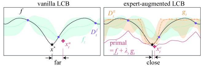
Figure 2: Visual explanation: While the vanilla LCB returns $x^{u}_{t}$, a far point from global minimum $x^{*}$, expert-augmented LCB can successfully navigate to closer point $x^{c}_{t}$ by mixing $f_{t}$ and $g_{t}$ with $\underline{f}_{t}+\lambda_{t}\underline{g}_{t}$, where $\lambda_{t}$ is the dual variable. In the figure, $D_{t}^{f}$ is the set of the sample points of the objective function $f$ and $D_{t}^{g}$ is the set of human feedback.

Primal dual. We introduce the following primal-dual problem (5) as our acquisition policy,

$$\textbf{Primal}:x^{c}_{t}\in\arg\min_{x\in\mathcal{X}}\underline{f}_{t}(x)+\lambda_{t}\underline{g}_{t}(x),\textbf{ Dual}:\lambda_{t+1}=[\lambda_{t}+{\zeta}\underline{g}_{t}(x_{t}^{c})]^{+},$$ (5)

where $\lambda_{t}$ is the primal-dual weight at the $t$-th iteration and ${\zeta}$ is the step size for dual update. See Fig. 2 for the intuition: we prioritise the sample in the expert-preferred region (i.e., the region with small $\underline{g}_{t}(x)$). The primal-dual method is a classical algorithm for constrained optimisation [63] and has recently been applied to, for example, the constrained bandit problem [109]. In terms of constrained optimisation, Prob. (5) can be understood as solving $\min_{x\in\mathcal{X}}\underline{f}(x)\,\,\text{s.t.}\,\,\underline{g}_{t}(x)\leq 0$. Interestingly, the primal-dual approach is also roughly analogous to Bayesian inference [25]. Just as the prior acts as a regulariser to the LL maximiser [93], expert belief $\underline{g}_{t}(x)$ regularises the $\underline{f}_{t}(x)$ minimiser. More specifically, the weight $\lambda_{t+1}$ increases when $\underline{g}_{t}(x_{t}^{c})>0$; otherwise, $\lambda_{t+1}$ decreases. The condition $\underline{g}_{t}(x_{t}^{c})>0$ indicates that the primal solution $x_{t}^{c}$ is more likely to be rejected. Under such a risk of rejection, increasing the weights $\lambda_{t+1}$ is natural because it more strongly regularises the $\underline{f}_{t}$ minimiser to enhance feasibility in the next round, and vice versa.

Level of trust. Note that the primal-dual method is not the primary reason we achieve the no-harm guarantee. Indeed, its proof (detailed later) does not rely on the primal-dual formulation. Therefore, technically speaking, our algorithm could employ a more aggressive exploitation of $g_{t}$ (e.g., simply minimising $g_{t}$). Nevertheless, the primal-dual approach is our recommended policy for generating the expert-augmented candidate $x^{c}_{t}$ to enhance resilience to erroneous inputs. The initial level of trust on $g_{t}$ is determined by the initial weight $\lambda_{0}$, where larger $\lambda_{0}$ values correspond to greater trust in the expert. We compared the effect of $\lambda_{0}$ in the later experimental section.

Efficient computation. Leveraging the representer theorem [76, 106] due to the RKHS property, we further reformulate Prob. (5) to a $(|\mathcal{Q}^{g}_{t}|+d+1)$-dimensional, tractable optimisation problem (6).

$$\min_{Z_{\mathcal{Q}^{g}_{t}}\in\mathbb{R}^{|\mathcal{Q}^{g}_{t}|},\,\,z\in\mathbb{R},\,\,x\in\mathcal{X}} \quad\underline{f}_{t}(x)+\lambda_{t}z$$ (6)

subject to $$\quad\left[\begin{array}[]{l}Z_{\mathcal{Q}^{g}_{t}}\\ z\end{array}\right]^{\top}K_{\mathcal{Q}^{g}_{t},x}^{-1}\left[\begin{array}[]{l}Z_{\mathcal{Q}^{g}_{t}}\\ z\end{array}\right]\leq B_{g}^{2},$$

$$\quad\ell(Z_{\mathcal{Q}^{g}_{t}}\mid\mathcal{D}^{g}_{t})\geq\ell_{t}(\hat{g}^{\mathrm{MLE}}_{t})-\alpha_{1}(\epsilon,\delta,|\mathcal{Q}^{g}_{t}|,t),$$

where $K_{\mathcal{Q}^{g}_{t},x}:=(k_{g}(\tilde{x},\tilde{x}^{\prime}))_{\tilde{x},\tilde{x}^{\prime}\in X_{\mathcal{Q}^{g}_{t}}\cup\{x\}}$, and $\ell(Z_{\mathcal{Q}^{g}_{t}}\mid\mathcal{D}^{g}_{t})=\sum_{\tau\in\mathcal{Q}^{g}_{t}}Z_{\tau}\mathbf{1}_{\tau}-\sum_{\tau\in\mathcal{Q}^{g}_{t}}\log\left(1+e^{Z_{\tau}}\right)$ is the LL value when $\hat{g}(x_{\tau})=Z_{\tau}$, $\forall\tau\in\mathcal{Q}^{g}_{t}$. We update $\lambda_{t+1}=\lambda_{t}+{\zeta}z^{\star}$, where $z^{\star}=\underline{g}_{t}(x_{t}^{c})$ is the optimal $z$ of Prob. (6).

Key hyperparameter estimation. A key hyperparameter in Prob. (6) is the norm bound $B_{g}$ in the first constraint. Another hyperparameter, $\alpha_{1}$, in the second constraint, also scales with $B_{g}$, (see Lemma 3.2). However, $B_{g}$ may be unknown in practice, and its mis-specification leads to mis-calibrated uncertainty. We estimate $B_{g}$ by starting with a small initial guess (e.g., 1) and doubling it when the following condition is met based on newly observed expert labels: $\alpha_{1}(\epsilon,\delta,|\mathcal{Q}^{g}_{t}|,t\mid 2\hat{B}_{g})<\ell_{t}(\hat{g}^{\mathrm{MLE}}_{t\mid 2\hat{B}_{g}})-\ell_{t}(\hat{g}^{\mathrm{MLE}}_{t\mid\hat{B}_{g}})$, where $\hat{B}_{g}$ is our current guess. Intuitively, if the new likelihood $\ell_{t}(\hat{g}^{\mathrm{MLE}}_{t\mid 2\hat{B}_{g}})$ is significantly larger, then $2\hat{B}_{g}$ is more likely a valid bound. We iterate this estimation online during optimisation and in pre-training with the initial dataset (see details in Appendix F).

4.2 Algorithm and Theoretical Guarantee

Algorithm. Our algorithm in Alg. 1 generates two candidates: the vanilla LCB $x^{u}_{t}$ and the expert-augmented LCB $x^{c}_{t}$. (See App. I.3 on extension to other acquisition functions.) Always selecting the vanilla LCB guarantees no-harm but misses the chance to accelerate convergence using the expert’s belief. Intuitively, this can be seen as a bandit problem regarding which arm to select. Line 8 corresponds to the handover guarantee, stating that our algorithm stops asking the expert once our model $g$ becomes more confident than the predefined $g_{\text{thr}}$. Line 6 outlines the conditions for achieving the no-harm guarantee by assessing the reliability of the expert-augmented candidate $x^{c}_{t}$. The first condition ensures $x^{c}_{t}$ is at least possibly better than the worst-case estimation of the optimal value. The second condition acts as active learning of human belief, exploring uncertain points to avoid inaccurate yet confident expert beliefs. The hyperparameter $\eta\geq 1$ represents the initial level of trust in the expert. A larger $\eta$ indicates greater priority in exploring expert-preferred regions.

Algorithm 1 COllaborative Bayesian Optimization with Labelling Experts (COBOL).

1:Input and Initialization: function space ball $\mathcal{B}_{g}$, trust weight $\eta$, and uncertainty threshold $g_{\textrm{thr}}$.

2:Set $\mathcal{B}^{1}_{g}=\mathcal{B}_{g}$, $\mathcal{Q}^{f}_{0}=\emptyset$, and $\mathcal{Q}^{g}_{0}=\emptyset$.

3:for $t\in[T]$ do

4:     Solve Prob. (5) via Prob. (6) to generate $x^{c}_{t}$. $\triangleright$ Expert-augmented LCB

5:     Solve the unconstrained problem, $x^{u}_{t}\in\arg\min_{x\in\mathcal{X}}\underline{f}_{t}(x).$ $\triangleright$ Vanilla LCB

6:     if $\underline{f}_{t}(x_{t}^{c})\leq\min_{x\in\mathcal{X}}\bar{f}_{t}(x)$ and $\sigma_{f_{t}}(x^{u}_{t})\leq\eta\sigma_{f_{t}}(x^{c}_{t})$  then $\triangleright$ No-harm guarantee

7:         Set $x_{t}=x_{t}^{c}$.

8:         if $\bar{g}_{t}(x_{t})-\underline{g}_{t}(x_{t})>g_{\textrm{thr}}$ then $\triangleright$ Handover guarantee

9:              Query the expert’s label to get the feedback $\mathbf{1}_{t}$.

10:              Update $\mathcal{Q}^{g}_{t}=\mathcal{Q}^{g}_{t-1}\cup\{t\}$ and the posterior confidence set $\mathcal{B}^{t+1}_{g}$.

11:              if $\mathbf{1}_{t}=1$ then

12:                  Set $\mathcal{Q}^{f}_{t}=\mathcal{Q}^{f}_{t-1}$, and continue the loop at line 4.                        

13:     else

14:         Set $\mathcal{Q}^{g}_{t}=\mathcal{Q}^{g}_{t-1}$, and $x_{t}=x_{t}^{u}$.      

15:     Evaluate the black-box function at the point $x_{t}$, and set $\mathcal{Q}^{f}_{t}=\mathcal{Q}^{f}_{t-1}\cup\{t\}$.

16:     Update the posterior mean/variance of the objective $f$.

Theoretical guarantee. For Alg. 1, we mainly care about two metrics: cumulative regret $R_{\mathcal{Q}^{f}_{T}}\vcentcolon=\sum_{t\in\mathcal{Q}^{f}_{T}}(f(x_{t})-f(x^{*}))$ and cumulative queries $Q^{g}_{T}\vcentcolon=|\mathcal{Q}^{g}_{T}|$. $R_{\mathcal{Q}^{f}_{T}}$ captures the cumulative regret over the query points to the black-box function. $Q^{g}_{T}$ captures the number of queries to the expert. Since intuitively each query to the expert causes inconvenience, ideally, the frequency of query to an expert should be low (e.g., $Q^{g}_{T}$ grows sublinearly in $T$).

Theorem 4.1.

Under Assumptions 2.1 to 2.6, with probability at least $1-\delta$, Alg 1 satisfies,

$$R_{\mathcal{Q}^{f}_{T}}\leq\mathcal{O}\left(\gamma_{|\mathcal{Q}^{f}_{T}|}^{f}\sqrt{|\mathcal{Q}^{f}_{T}|}\right),$$ (7a) (7b)

See Appendix B for the proof of Thm. 4.1. Intuitively, Eq. (7a) shows the no-harm guarantee, since it provides a cumulative regret bound independent of the latent function $g$. Eq. (7b) shows the handover guarantee, since the bound on cumulative queries to the expert is sublinear for commonly-used kernel functions (See Table 1). This means that the frequency of querying the expert asymptotically converges to zero. Since $\mathcal{Q}^{g}_{T}\cup\mathcal{Q}^{f}_{T}=[T]$, $|\mathcal{Q}^{f}_{T}|$ grows linearly in $T$. It should be noted that there is a trade-off in $\eta$ selection. A larger $\eta$ can accelerate convergence when feedback is informative, but it may also cause the worse convergence rate for adversarial feedback (see Appendix B, which includes an additional constant factor of $\nicefrac{{(2+\eta)}}{{4}}$ compared to the original UCB). In practice, setting $\eta=3$ is sufficiently effective (see Figure 3).

By plugging in the maximum information gain bounds [83, 92] and covering number bounds [103, 104, 18, 108], we apply Thm. 4.1 to derive the kernel-specific bounds in Table 1. In practice, kernel choice and scalability to high dimensions are common challenges for BO. Existing generic techniques, such as decomposed kernels [48], can be applied in our algorithm to choose kernel functions and achieve scalability in high-dimensional spaces.

Table 1: Kernel-specific bounds where $\nu$ is the smoothness parameter of the Matérn kernel that is assumed to satisfy $\nu>\frac{d}{4}(3+d+\sqrt{d^{2}+14d+17})=\Theta(d^{2})$.

Metric	Linear	Squared Exponential	Matérn
$R_{\mathcal{Q}^{f}_{T}}$	$\mathcal{O}\left(\sqrt{|\mathcal{Q}^{f}_{T}|}\log|\mathcal{Q}^{f}_{T}|\right)$	$\mathcal{O}\left(\sqrt{|\mathcal{Q}^{f}_{T}|}(\log|\mathcal{Q}^{f}_{T}|)^{d+1}\right)$	$\mathcal{O}\left(|\mathcal{Q}^{f}_{T}|^{\frac{2\nu+3d}{4\nu+2d}}\log^{\frac{2\nu}{2\nu+d}}(|\mathcal{Q}^{f}_{T}|)\right)$
$Q^{g}_{T}$	$\mathcal{O}\left((\log T)^{3}\right)$	$\mathcal{O}\left((\log T)^{3(d+1)}\right)$	$\mathcal{O}(T^{\frac{2d(d+1)}{2\nu+d(d+1)}}T^{\frac{d}{\nu}}(\log T)^{3})$

4.3 Related Works

Human-AI Collaborative BO. There are two primary approaches: the first approach assumes that human experts can express their beliefs through quantitative labels, such as well-defined distributions [68, 51, 81, 42, 24, 41] or pinpoint querying locations [11, 38, 49, 12, 69]. While this strong assumption is valid in specific cases, such as physics simulations [38], many experimental tasks—such as chemistry, which lacks the consensus on numerical representations of, e.g. molecules—require more relaxed assumptions [24, 45]. The qualitative approach, on the other hand, involves human experts providing pairwise comparisons [7] or binary recommendations (ours). The algorithm trains a surrogate model from experts’ labels, thereby expanding applicable scenarios. Ours is the first-of-its-kind principled method with both no-harm and handover guarantee on a continuous domain.

Related BO tasks. Eliciting human preference from labels has been explored in preferential BO [28, 36, 58, 90, 9, 106]. However, this approach treats human preference as the main objective of BO, whereas our work uses experts’ belief as an additional information source. Constrained BO [32, gelbart2014bayesian, 87, 86, 109, 105, 61, 43, 95, 56] is another line of research that investigates BO under unknown constraints, placing another surrogate model on the constraint inferred from queried labels. However, our approach does not treat human belief as a constraint that must be satisfied or a reward to maximise, given that expert knowledge can sometimes be unreliable (see details in Appendix G).

5 Experiments

We benchmarked the performance of the proposed algorithm against existing baselines in a collaborative setting with human experts. We employed an ARD RBF kernel for both $f$ and $g$. In each iteration of the optimisation loop, the inputs were rescaled to the unit cube $[0,1]^{d}$, and the outputs were standardised to have zero mean and unit variance. The initial datasets consisted of three random data points sampled uniformly from within the domain, and in each iteration, one data point was queried. Additionally, we collected initial expert labels by asking an expert to label ‘accept’ (= 0) or ‘reject’ (= 1) for 10 uniformly random points. All experiments were repeated ten times with different initial datasets and random seeds. We tuned hyperparameters online at each iteration. The GP hyperparameters were tuned by maximising the marginal likelihood on observed datasets using a multi-start L-BFGS-B method [52] (the default BoTorch optimiser [14]). The key hyperparameters of the confidence set, $B_{g}$ and $\alpha_{1}$, were optimised via the online method in Appendix F. Other hyperparameters were set as $\eta=3$, $\lambda_{0}=1$, and $g_{\text{thr}}=0.1$ by default throughout the experiments, with their sensitivity discussed later (see also Appendix J.1). The constrained optimisation in Prob. (6) was solved using the interior-point nonlinear optimiser IPOPT [94], which is highly scalable for solving the primal problem, via the symbolic interface CasADi [8]. The unconstrained optimisation (line 5) was solved using the default BoTorch optimiser [14]. More details for reproducing results are available on GitHub. The models were implemented in GPyTorch [31]. All experiments were conducted on a laptop PC. Computational time is discussed in Appendix J. In addition to cumulative regret and queries, we also consider simple regret defined as $\text{SR}_{t}:=\min_{\tau\in\mathcal{Q}^{f}_{t}}(f(x_{\tau})-f(x^{\star}))$.

Robustness and sensitivity.

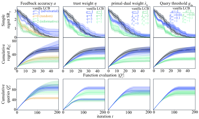
Figure 3: Robustness and sensitivity analysis using the Ackley function. Lines and shaded areas denote mean $\pm$ 1 standard error. The no-harm guarantee ensures the convergence rate is on par with vanilla LCB even in adversarial cases. Handover guarantee ensures that $\mathcal{Q}^{g}_{t}$ plateau, allowing optimisation without expert intervention once sufficient information has been elicited.

First, we tested the robustness of our algorithm to the accuracy of the expert’s labels using the 4-dimensional Ackley function [1]. We modelled the synthetic agent response according to Example 2.2. In particular, we examine the impact of feedback accuracy, denoted as $a$. Fig. 3 illustrates the robustness of our algorithm. When labels are informative ($a=1,2$), the convergence rate for both simple and cumulative regrets is accelerated in accordance with the accuracy. Even if the feedback is completely random ($a=0$) or adversarial ($a=-1,-2$), the no-harm guarantee ensures that the algorithm converges at a rate on par with vanilla LCB by adjusting the level of trust to be lower over iterations. Refer to Appendix J.2.3 for additional confirmation of the no-harm guarantee based on more extensive experimental results. Handover guarantee ensures that our algorithm stops seeking label feedback once sufficient information has been elicited, as indicated by the plateau in the cumulative queries $Q^{g}_{T}$. We also tested the sensitivity to the optimisation parameters $\eta,\lambda_{0}$, and $g_{\text{thr}}$. The change in convergence at those parameters were varied mostly within the standard error, indicating that our algorithm is insensitive to these hyperparameters and that feedback accuracy is more dominant. For the primal-dual weight, $\lambda_{0}=0$ corresponds to constrained optimisation without a primal-dual mixing objective, which performs worse than mixing cases ($\lambda_{0}=1,2$), demonstrating the efficacy of incorporating the primal-dual mixing objective.

Synthetic dataset.

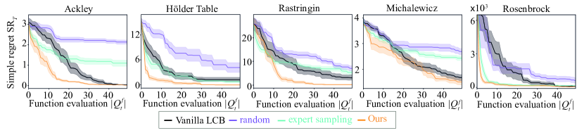
Figure 4: Ablation study on five common synthetic functions with synthetic expert labels ($a=1$).

We compared our algorithm against five common synthetic functions [88] (see details in Appendix J.2), using simple baselines for an ablation study: random sampling, vanilla LCB (unconstrained optimisation), and expert sampling. Expert sampling involves direct sampling from the expert belief distribution $p_{x\succ_{g}0}$. We employ rejection sampling by generating a uniform random sample over the domain and then accepting it with the probability $1-p_{x\succ_{g}0}$. We fixed the feedback accuracy at $a=1$ (as in Example 2.2.). The efficacy of expert labels is roughly estimated by how much faster expert sampling converges compared to random sampling. In all synthetic experiments, our algorithm outperformed the baselines. While expert sampling is at least more effective than random sampling, it is not always better than vanilla LCB. For functions with a very sharp global optimum, such as Rosenbrock [70], $p_{x\succ_{g}0}$ nearly pinpoints the global minimum. Still, our algorithm performs slightly better than expert sampling. See Appendix J.2.2 for computation time and query frequency. The overhead of our algorithm is comparable to that of other baselines.

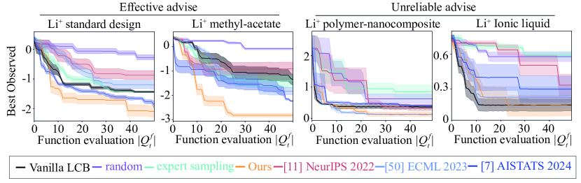
Figure 5: Real-world experiments with four human experts of lithium-ion batteries.

Real-world experiments with human experts. We conducted real-world experiments in collaboration with four human experts who possess post-doctoral level knowledge on lithium-ion batteries. In this experiment, human labelling costs vary among experts but typically range from a few seconds to several minutes. In the real-world development of lithium-ion batteries, creating and testing a prototype cell requires at least a week, making the labelling cost negligible by comparison.

Lithium-ion batteries are crucial for realising a green society, a rapidly growing field where knowledge is continuously updated at an unprecedented rate. This field typically suffers from data scarcity [45] due to the ongoing development of new materials synthesised by chemists. Consequently, transfer learning approaches, e.g., [89, 100, 30, 21], are not effective in this setting. We prepared four cases for the experiments: the first is a standard task where we optimise the standard electrolyte composition [26, 35], and the second involves a slight modification of the first setup by changing one solvent material [55]. We expect the experts to have informative knowledge on these two tasks. The remaining two cases involve emerging new categories of materials: one is a polymer-nanocomposite electrolyte [107], and the other is an ionic liquid [71]. We anticipate that the experts’ knowledge on these new materials will not be as effective as in the first two tasks (see more details in Appendix J.3). Given the scarcity of real experts, we conducted a pre-experimental step to elicit their knowledge for a fair baseline comparison. We asked them to label 50 random points uniformly from the domain, for all experiments before seeing the results. Then we fit the confidence set model to these results and used $\hat{g}_{t}^{\text{MLE}}$ as the estimated human response. Additionally, we asked the participants to manually select the next query point without any assistance from BO, which we refer to as ‘expert sampling’ in the baseline. We also compared against state-of-the-art algorithms [11, 49, 7]. These methods have predefined levels of trust, roughly ranked from strong to weak: [11] $\rightarrow$ [7] $\rightarrow$ [49]. Ours can adjust the level of trust based on data, so we expect it to perform well in both effective and ineffective cases.

Fig. 5 summarises the results. For the first two tasks, our algorithm outperformed all baselines. Particularly in the second task, human sampling was better than vanilla LCB, indicating that we should trust their advice aggressively. Our algorithm can adapt to trust them over time, resulting in significantly accelerated convergence. On the other hand, expert sampling for the new materials tasks was, although unintentionally, worse than random, thereby discouraging trust. While trustful algorithms [11, 7] struggled to converge, the distrustful algorithm [49] was able to converge on par with vanilla LCB. Our no-harm guarantee worked in this situation, gradually equating to LCB, and showed identical performance to the distrustful algorithm [49]. See also Appendix J.4.1 for the complete experimental results on the number of queries and computation time.

6 Discussion

Feedback form. Other forms of feedback, such as pairwise comparisons [7] or preferential rankings [12], can be incorporated into our algorithm with slight modifications. However, we empirically found that the binary labelling approach performs best (see Fig. 5), and therefore, we recommend using binary feedback as the primary choice. For those interested in using alternative feedback forms, detailed instructions on how to adapt them to our algorithm are provided in Appendix H.

Time-varying human knowledge. We assume that expert knowledge is stationary, although it can be time-varying, e.g., experts’ knowledge often evolves as more data is gathered. A simple extension to accommodate this is the use of windowing, where past queried data is forgotten. This can be easily implemented in our algorithm by removing old data beyond a predefined iteration window. However, our initial trials did not show significant performance gains from this approach, so it was not included in the main text. We suggest a dynamic model as a potential future direction, which is discussed in Appendix I.1 with additional experimental results. Similarly, we kept the trust weight $\eta$ fixed throughout the optimization process. Since human knowledge can improve over time, an adaptive $\eta$ could be employed to enhance both convergence and robustness. Nevertheless, our no-harm guarantee remains valid even without this adaptation. Further details are provided in Appendix I.2.

Acceleration vs. Robustness. One might seek to derive a theoretical guarantee on the acceleration of convergence when the feedback is helpful. However, we want to emphasize that theoretically guaranteeing both acceleration and robustness may be incompatible. From a theoretical perspective, they are in a trade-off relationship [91]. This can be intuitively explained by the no-free-lunch theorem [101]: if algorithm A outperforms B, it does so by exploiting ‘biased’ information. The ‘bias’ inherent in the acceleration is contradictory to robustness. Our setting is unbiased, meaning we do not have prior knowledge of helpful or adversarial human expert. Therefore, we must make a design choice between prioritizing robustness or acceleration as a theoretical contribution, depending on whether we assume that expert input can be adversarial (weak bias) or that it will always be helpful (strong bias). Indeed, there are lower bound results for the average-case regret of Bayesian optimization in the literature (e.g., see [75]). GP-UCB is already nearly rate-optimal in achieving this lower bound. This means theoretical acceleration is obtained in the price of worse robustness. In Appendix E, we present a slightly modified version, Algorithm 2, which offers an improvement guarantee based on strong bias. Our Algorithm 1 can be seen as a relaxed version of this algorithm (soft constraint), which helps explain the empirical success in accelerating convergence.

7 Conclusion

Our algorithm, with its data-driven adjustment of the level of trust, successfully accelerated convergence from effective advice while ensuring a no-harm guarantee from unreliable inputs. The handover guarantee also ensures that the BO can automate the optimisation process without assistance from human experts at a later stage. These features are particularly valuable for scientific applications, where researchers often face trial and error, making it challenging to determine the effectiveness of their prior knowledge before starting experiments. Our flexible and robust framework is also expected to be effective in collaboration with large language models (LLMs), which demonstrate remarkable sample-efficient performance by exploiting encoded priors [54, 74, 65], and can be regarded as ‘expert knowledge’. Our safeguard features would be particularly effective for shared challenges, such as difficulty in eliciting knowledge [44, 16] and varying accuracy of advice due to hallucinations [80, 97, 84]. Although ours is the first-of-its-kind algorithm with a general theoretical guarantee in the expert-collaborative setting, it is still based on the GP-UCB algorithm  and shares its limitations (e.g., high dimensionality). One future direction is combining our approach with the high-dimensional BO methods [96, 50]. Additionally, our current setting does not consider the batch setting, yet one can easily extend with existing approaches, e.g. [4, 6, 3, 5]. Multiple expert scenario is also a promising future extension. While a simple expert aggregation approach (e.g., majority vote, adding multiple experts $g$) could work without modifications to the current algorithm, more advanced methods, such as choice functions [15], present promising directions for future work. Our method can positively influence human experts by empirically demonstrating the value of their expertise, even amidst concerns about job security in the AI era [13]. On the negative side, more powerful LLMs may eventually replace the expert role in our algorithm in areas where data is sufficiently shared on websites or in papers, such as hyperparameter tuning [54].

Part I Appendix

Appendix A Proof of Lem. 3.2

To prepare for the proof of the lemma, we first prove several preliminary lemmas.

Lemma A.1.

For any fixed $\hat{g}\in\mathcal{B}_{g}$, we have,

$$\mathbb{P}\left(\log\mathbb{P}_{\hat{g}}((x_{\tau},\mathbf{1}_{\tau})_{\tau\in\mathcal{Q}^{g}_{t}})-\log\mathbb{P}_{{g}}((x_{\tau},\mathbf{1}_{\tau})_{\tau\in\mathcal{Q}^{g}_{t}})\leq\sqrt{8|\mathcal{Q}^{g}_{t}|B_{f}^{2}\log\frac{1}{\delta_{t}}}\right)\geq 1-\delta_{t}.$$ (8)

Proof.

We use $u_{\tau}$ to denote $g(x_{\tau})$, $z_{\tau}$ to denote $\hat{g}(x_{\tau})$, and $p_{\tau}$ to denote $S(g(x_{\tau}))$.

$$\mathbb{P}\left(\log\mathbb{P}_{\hat{g}}((x_{\tau},\mathbf{1}_{\tau})_{\tau\in\mathcal{Q}^{g}_{t}})-\log\mathbb{P}_{{g}}((x_{\tau},\mathbf{1}_{\tau})_{\tau\in\mathcal{Q}^{g}_{t}})\leq\xi\right)$$ (9)

$$= \mathbb{P}\left(\sum_{\tau\in\mathcal{Q}^{g}_{t}}\left((z_{\tau}-u_{\tau})\mathbf{1}_{\tau}-\log(1+e^{z_{\tau}})+\log(1+e^{u_{\tau}})\right)\leq\xi\right)$$ (10)

$$= \mathbb{P}\left(\sum_{\tau\in\mathcal{Q}^{g}_{t}}(z_{\tau}-u_{\tau})\mathbf{1}_{\tau}-\sum_{\tau\in\mathcal{Q}^{g}_{t}}(z_{\tau}-u_{\tau})p_{\tau}\leq\xi^{\prime}\right)$$ (11)

where the probability $\mathbb{P}$ is taken over the randomness from the feedback expert/oracle and the randomness from the algorithm, and $\xi^{\prime}=\xi+\sum_{\tau\in\mathcal{Q}^{g}_{t}}\log\left(1+e^{z_{\tau}}\right)-\sum_{\tau\in\mathcal{Q}^{g}_{t}}\log\left(1+e^{u_{\tau}}\right)-\sum_{\tau\in\mathcal{Q}^{g}_{t}}(z_{\tau}-u_{\tau})p_{\tau}$. Let the function $\psi_{\tau}(z_{\tau})\vcentcolon=\log\left(1+e^{z_{\tau}}\right)-\log\left(1+e^{u_{\tau}}\right)-(z_{\tau}-u_{\tau})p_{\tau}$. It can be checked that $\psi_{\tau}^{{}^{\prime\prime}}(z_{\tau})=\nicefrac{{e^{z_{\tau}}}}{{(1+e^{z_{\tau}})^{2}}}\geq 0,\forall z_{\tau}\in\mathbb{R}$ and $\psi_{\tau}^{{}^{\prime}}(u_{\tau})=0$. Therefore, $\psi_{\tau}$ is a convex function and achieves the optimal value at the point $u_{\tau}$. Hence, $\psi_{\tau}(z_{\tau})\geq\psi_{\tau}(u_{\tau})=0$, which implies $\xi^{\prime}\geq\xi$. Therefore,

$$\mathbb{P}\left(\sum_{\tau\in\mathcal{Q}^{g}_{t}}(z_{\tau}-u_{\tau})\mathbf{1}_{\tau}-\sum_{\tau\in\mathcal{Q}^{g}_{t}}(z_{\tau}-u_{\tau})p_{\tau}\leq\xi^{\prime}\right)\geq\mathbb{P}\left(\sum_{\tau\in\mathcal{Q}^{g}_{t}}(z_{\tau}-u_{\tau})\mathbf{1}_{\tau}-\sum_{\tau\in\mathcal{Q}^{g}_{t}}(z_{\tau}-u_{\tau})p_{\tau}\leq\xi\right).$$ (12)

Furthermore, it is easy to see that $(z_{\tau}-u_{\tau})\mathbf{1}_{\tau}\in[-2B_{g},2B_{g}]$, and thus, by applying Azuma-Hoeffding inequality, we have,

$$\mathbb{P}\left(\sum_{\tau\in\mathcal{Q}^{g}_{t}}(z_{\tau}-u_{\tau})\mathbf{1}_{\tau}-\sum_{\tau\in\mathcal{Q}^{g}_{t}}(z_{\tau}-u_{\tau})p_{\tau}\leq\xi\right)\geq 1-\exp\left\{-\frac{\xi^{2}}{8|\mathcal{Q}^{g}_{t}|B_{g}^{2}}\right\}$$ (13)

Let $\exp\left\{-\frac{\xi^{2}}{8|\mathcal{Q}^{g}_{t}|B_{g}^{2}}\right\}\leq\delta_{t}$, we need,

$$\xi\geq\sqrt{8|\mathcal{Q}^{g}_{t}|B_{g}^{2}\log\frac{1}{\delta_{t}}}.$$ (14)

It is sufficient to pick $\xi=\sqrt{8|\mathcal{Q}^{g}_{t}|B_{g}^{2}\log\frac{1}{\delta_{t}}}$. Therefore,

$$\mathbb{P}\left(\log\mathbb{P}_{\hat{g}}((x_{\tau},\mathbf{1}_{\tau})_{\tau\in\mathcal{Q}^{g}_{t}})-\log\mathbb{P}_{{g}}((x_{\tau},\mathbf{1}_{\tau})_{\tau\in\mathcal{Q}^{g}_{t}})\leq\sqrt{8|\mathcal{Q}^{g}_{t}|B_{g}^{2}\log\frac{1}{\delta_{t}}}\right)$$

$$\geq \mathbb{P}\left(\sum_{\tau\in\mathcal{Q}^{g}_{t}}(z_{\tau}-u_{\tau})\mathbf{1}_{\tau}-\sum_{\tau\in\mathcal{Q}^{g}_{t}}(z_{\tau}-u_{\tau})p_{\tau}\leq\sqrt{8|\mathcal{Q}^{g}_{t}|B_{g}^{2}\log\frac{1}{\delta_{t}}}\right)$$

$$\geq 1-\delta_{t},$$

where the first inequality follows by combining Eq. (11) and Eq. (12).

∎

We then have the following high probability confidence set lemma.

Lemma A.2.

For any fixed $\hat{g}$ that is independent of $((x_{\tau},\mathbf{1}_{\tau})_{\tau\in\mathcal{Q}^{g}_{t}})$, we have, with probability at least $1-\delta$, $\forall t\geq 1$,

$$\log\mathbb{P}_{\hat{g}}((x_{\tau},\mathbf{1}_{\tau})_{\tau\in\mathcal{Q}^{g}_{t}})-\log\mathbb{P}_{{g}}((x_{\tau},\mathbf{1}_{\tau})_{\tau\in\mathcal{Q}^{g}_{t}})\leq\sqrt{8|\mathcal{Q}^{g}_{t}|B_{g}^{2}\log\frac{\pi^{2}t^{2}}{6\delta}}.$$ (15)

Proof.

We use $\mathcal{E}_{t}$ to denote the event $\log\mathbb{P}_{\hat{g}}((x_{\tau},\mathbf{1}_{\tau})_{\tau\in\mathcal{Q}^{g}_{t}})-\log\mathbb{P}_{{g}}((x_{\tau},\mathbf{1}_{\tau})_{\tau\in\mathcal{Q}^{g}_{t}})\leq\sqrt{8|\mathcal{Q}^{g}_{t}|B_{g}^{2}\log\frac{1}{\delta_{t}}}$. We pick $\delta_{t}=\nicefrac{{(6\delta)}}{{(\pi^{2}t^{2})}}$ and have,

$$\mathbb{P}\left(\log\mathbb{P}_{\hat{g}}((x_{\tau},\mathbf{1}_{\tau})_{\tau\in\mathcal{Q}^{g}_{t}})-\log\mathbb{P}_{{g}}((x_{\tau},\mathbf{1}_{\tau})_{\tau\in\mathcal{Q}^{g}_{t}})\leq\sqrt{8|\mathcal{Q}^{g}_{t}|B_{g}^{2}\log\frac{1}{\delta_{t}}},\forall t\geq 1\right)$$

$$= 1-\mathbb{P}\left(\overline{\cap_{t=1}^{\infty}\mathcal{E}_{t}}\right)$$

$$= 1-\mathbb{P}\left({\cup_{t=1}^{\infty}\overline{\mathcal{E}_{t}}}\right)$$

$$\geq 1-\sum_{t=1}^{\infty}\mathbb{P}\left(\overline{\mathcal{E}_{t}}\right)$$

$$= 1-\sum_{t=1}^{\infty}\left(1-\mathbb{P}\left({\mathcal{E}_{t}}\right)\right)$$

$$= 1-\sum_{t=1}^{\infty}\left(1-\mathbb{P}\left({\log\mathbb{P}_{\hat{g}}((x_{\tau},\mathbf{1}_{\tau})_{\tau\in\mathcal{Q}^{g}_{t}})-\log\mathbb{P}_{{g}}((x_{\tau},\mathbf{1}_{\tau})_{\tau\in\mathcal{Q}^{g}_{t}})\leq\sqrt{8|\mathcal{Q}^{g}_{t}|B_{g}^{2}\log\frac{1}{\delta_{t}}}}\right)\right)$$

$$\geq 1-\sum_{t=1}^{\infty}\delta_{t}$$

$$= 1-\frac{6\delta}{\pi^{2}}\sum_{t=1}^{\infty}\frac{1}{t^{2}}$$

$$= 1-\delta.$$

∎

We then have a lemma to bound the difference of log likelihood when two functions are close in infinity-norm sense.

Lemma A.3.

$\forall\epsilon>0$, $\forall g_{1},g_{2}\in\mathcal{B}_{g}$ that satisfies $\|g_{1}-g_{2}\|_{\infty}\leq\epsilon$, we have,

$$\log\mathbb{P}_{{g}_{1}}((x_{\tau},\mathbf{1}_{\tau})_{\tau\in\mathcal{Q}^{g}_{t}})-\log\mathbb{P}_{{g}_{2}}((x_{\tau},\mathbf{1}_{\tau})_{\tau\in\mathcal{Q}^{g}_{t}})\leq 2\epsilon|\mathcal{Q}^{g}_{t}|.$$ (16)

Proof.

$$\log\mathbb{P}_{{g}_{1}}((x_{\tau},\mathbf{1}_{\tau})_{\tau\in\mathcal{Q}^{g}_{t}})-\log\mathbb{P}_{{g}_{2}}((x_{\tau},\mathbf{1}_{\tau})_{\tau\in\mathcal{Q}^{g}_{t}})$$

$$\leq \sum_{\tau\in\mathcal{Q}^{g}_{t}}\left((z_{1,\tau}-z_{2,\tau})\mathbf{1}_{\tau}-\log(1+e^{z_{1,\tau}})+\log(1+e^{z_{2,\tau}})\right)$$

$$\leq \epsilon|\mathcal{Q}^{g}_{t}|+\sum_{\tau\in\mathcal{Q}^{g}_{t}}\max_{z\in[-B_{g},B_{g}]}\left|\nabla_{z}\log\left(1+e^{z}\right)\right|\left|z_{1,\tau}-z_{2,\tau}\right|$$

$$\leq \epsilon|\mathcal{Q}^{g}_{t}|+\sum_{\tau\in\mathcal{Q}^{g}_{t}}\epsilon$$

$$\leq 2\epsilon|\mathcal{Q}^{g}_{t}|,$$

where $z_{1,\tau}=g_{1}(x_{\tau})$ and $z_{2,\tau}=g_{2}(x_{\tau})$. ∎

We use $\mathcal{N}(\mathcal{B}_{g},\epsilon,\|\cdot\|_{\infty})$ to denote the covering number of the set $\mathcal{B}_{g}$, with $(g^{\epsilon}_{i})_{i=1}^{\mathcal{N}(\mathcal{B}_{g},\epsilon,\|\cdot\|_{\infty})}$ be a set of $\epsilon$-covering for the set $\mathcal{B}_{g}$. Set the ‘$\delta$’ in Lem. A.2 as $\nicefrac{{\delta}}{{\mathcal{N}(\mathcal{B}_{g},\epsilon,\|\cdot\|_{\infty})}}$ and applying the probability union bound, we have, with probability at least $1-\delta$, $\forall g_{i}^{\epsilon}$,

$$\log\mathbb{P}_{{g}_{i}^{\epsilon}}((x_{\tau},\mathbf{1}_{\tau})_{\tau\in\mathcal{Q}^{g}_{t}})-\log\mathbb{P}_{{g}}((x_{\tau},\mathbf{1}_{\tau})_{\tau\in\mathcal{Q}^{g}_{t}})\leq\sqrt{8|\mathcal{Q}^{g}_{t}|B_{g}^{2}\log\frac{\pi^{2}t^{2}\mathcal{N}(\mathcal{B}_{g},\epsilon,\|\cdot\|_{\infty})}{6\delta}}.$$ (17)

By the definition of $\epsilon$-covering, there exists $j\in[\mathcal{N}(\mathcal{B}_{g},\epsilon,\|\cdot\|_{\infty})]$, such that,

$$\|\hat{g}_{t+1}^{\mathrm{MLE}}-g_{j}^{\epsilon}\|_{\infty}\leq\epsilon.$$ (18)

Hence, with probability at least $1-\delta$,

$$\log\mathbb{P}_{\hat{g}_{t+1}^{\mathrm{MLE}}}((x_{\tau},\mathbf{1}_{\tau})_{\tau\in\mathcal{Q}^{g}_{t}})-\log\mathbb{P}_{{g}}((x_{\tau},\mathbf{1}_{\tau})_{\tau\in\mathcal{Q}^{g}_{t}})$$

$$= \log\mathbb{P}_{\hat{g}_{t+1}^{\mathrm{MLE}}}((x_{\tau},\mathbf{1}_{\tau})_{\tau\in\mathcal{Q}^{g}_{t}})-\log\mathbb{P}_{{g}_{j}^{\epsilon}}((x_{\tau},\mathbf{1}_{\tau})_{\tau\in\mathcal{Q}^{g}_{t}})+\log\mathbb{P}_{{g}_{j}^{\epsilon}}((x_{\tau},\mathbf{1}_{\tau})_{\tau\in\mathcal{Q}^{g}_{t}})-\log\mathbb{P}_{{g}}((x_{\tau},\mathbf{1}_{\tau})_{\tau\in\mathcal{Q}^{g}_{t}})$$

$$\leq 2\epsilon|\mathcal{Q}^{g}_{t}|+\sqrt{8|\mathcal{Q}^{g}_{t}|B_{g}^{2}\log\frac{\pi^{2}t^{2}\mathcal{N}(\mathcal{B}_{g},\epsilon,\|\cdot\|_{\infty})}{6\delta}},$$

where the inequality follows by Lem. A.3 and Lem. A.2.

Appendix B Proof of Thm. 4.1

B.1 Bound Error over Historical Evaluations

Lem. 3.2 gives a high confidence set based on the likelihood function. The following Lem. B.1 further gives error bound over the historical sample points. Lem. B.1 highlights that with high probability, all the functions in the confidence set have values over the historical sample points that lie in a ball with the ground-truth function value as the center and $\sqrt{\alpha(\epsilon,\nicefrac{{\delta}}{{2}},|\mathcal{Q}^{g}_{t}|,t)}$ as the radius. Before we proceed, we first introduce several constants that we will use,

$$\bar{S}\vcentcolon=\max_{u\in[-B_{g},B_{g}]}S(u)=\frac{1}{1+e^{-B_{g}}},\underline{S}\vcentcolon=\min_{u\in[-B_{g},B_{g}]}S(u)=\frac{1}{1+e^{B_{g}}}.$$ (19)

$$\underline{S^{\prime}}\vcentcolon=\min_{u\in[-B_{g},B_{g}]}S^{\prime}(u)=\frac{1}{e^{B_{g}}+e^{-B_{g}}+2},\bar{S^{\prime}}\vcentcolon=\max_{u\in[-B_{g},B_{g}]}S^{\prime}(u)=\frac{1}{4}.$$ (20)

$$H_{S}\vcentcolon=\frac{1}{2\bar{S}^{2}},B_{p}=\frac{S(B_{g})}{S(-B_{g})}-\frac{S(-B_{g})}{S(B_{g})}.$$ (21)

Lemma B.1.

For any estimate $\hat{g}_{t+1}\in\mathcal{B}_{g}^{t+1}$ that is measurable with respect to the filtration $\mathcal{F}_{t}$, we have, with probability at least $1-\nicefrac{{\delta}}{{2}}$, $\forall t\geq 1$,

$$\sum_{\tau\in\mathcal{Q}^{g}_{t}}\left(\hat{g}_{t+1}(x_{\tau})-{g}(x_{\tau})\right)^{2}\leq\alpha(\epsilon,\nicefrac{{\delta}}{{2}},|\mathcal{Q}^{g}_{t}|,t),$$ (22)

and

$$g\in\mathcal{B}_{g}^{t+1},$$ (23)

where $\alpha(\epsilon,\nicefrac{{\delta}}{{2}},|\mathcal{Q}^{g}_{t}|,t)=\frac{\underline{S^{\prime}}^{2}}{H_{S}}\left(\alpha_{2}(\epsilon,\nicefrac{{\delta}}{{2}},|\mathcal{Q}^{g}_{t}|,t)+2\alpha_{1}(\epsilon,\nicefrac{{\delta}}{{2}},|\mathcal{Q}^{g}_{t}|,t)\right)=\mathcal{O}\left(\sqrt{|\mathcal{Q}^{g}_{t}|\log\frac{t\mathcal{N}(\mathcal{B}_{g},\epsilon,\|\cdot\|_{\infty})}{\delta}}+\epsilon t+\epsilon^{2}t\right)$, with $\alpha_{2}(\epsilon,\delta,|\mathcal{Q}^{g}_{t}|,t)=8H_{S}\bar{S^{\prime}}^{2}\epsilon^{2}t+4\epsilon t+\sqrt{8{|\mathcal{Q}^{g}_{t}|B_{p}^{2}\log\frac{\pi^{2}t^{2}\mathcal{N}(\mathcal{B}_{g},\epsilon,\|\cdot\|_{\infty})}{3\delta}}{}}$.

Proof.

For any fixed function $\hat{g}$, we have,

$$\log{\mathbb{P}_{\hat{g}}}((x_{\tau},\mathbf{1}_{\tau})_{\tau\in\mathcal{Q}^{g}_{t}})-\log{\mathbb{P}_{{g}}}((x_{\tau},\mathbf{1}_{\tau})_{\tau\in\mathcal{Q}^{g}_{t}})$$

$$= \sum_{\tau\in\mathcal{Q}^{g}_{t}}\left(\log{\mathbb{P}_{\hat{g}}}((x_{\tau},\mathbf{1}_{\tau}))-\log{\mathbb{P}_{{g}}}((x_{\tau},\mathbf{1}_{\tau}))\right)$$

$$= \sum_{\tau\in\mathcal{Q}^{g}_{t}}\left(\mathbf{1}_{\tau}\left(\log{\hat{p}_{\tau}}-\log{p}_{\tau}\right)+(1-\mathbf{1}_{\tau})\left(\log{(1-\hat{p}_{\tau})}-\log(1-{p}_{\tau})\right)\right),$$

where $\hat{p}_{\tau}=S(\hat{g}(x_{\tau}))$ and ${p}_{\tau}=S({g}(x_{\tau}))$. We have,

$$\log y\leq\log x+\frac{1}{x}(y-x)-H_{S}(y-x)^{2},\forall x,y\in[\underline{S},\bar{S}],$$ (24)

where $H_{S}=\frac{1}{2\bar{S}^{2}}$. Hence,

$$\log{\mathbb{P}_{\hat{g}}}((x_{\tau},\mathbf{1}_{\tau})_{\tau\in\mathcal{Q}^{g}_{t}})-\log{\mathbb{P}_{{g}}}((x_{\tau},\mathbf{1}_{\tau})_{\tau\in\mathcal{Q}^{g}_{t}})$$

$$= \sum_{\tau\in\mathcal{Q}^{g}_{t}}\left(\mathbf{1}_{\tau}\left(\log{\hat{p}_{\tau}}-\log{p}_{\tau}\right)+(1-\mathbf{1}_{\tau})\left(\log{(1-\hat{p}_{\tau})}-\log(1-{p}_{\tau})\right)\right)$$

$$\leq \sum_{\tau\in\mathcal{Q}^{g}_{t}}\left(\mathbf{1}_{\tau}\left(\frac{\hat{p}_{\tau}-p_{\tau}}{p_{\tau}}-H_{S}\left(\hat{p}_{\tau}-p_{\tau}\right)^{2}\right)+(1-\mathbf{1}_{\tau})\left(\frac{{p}_{\tau}-\hat{p}_{\tau}}{1-p_{\tau}}-H_{S}\left(\hat{p}_{\tau}-p_{\tau}\right)^{2}\right)\right)$$

Rearrangement gives,

$$H_{S}\sum_{\tau\in\mathcal{Q}^{g}_{t}}\left(\hat{p}_{\tau}-p_{\tau}\right)^{2}+\log{\mathbb{P}_{\hat{g}}}((x_{\tau},\mathbf{1}_{\tau})_{\tau\in\mathcal{Q}^{g}_{t}})-\log{\mathbb{P}_{{g}}}((x_{\tau},\mathbf{1}_{\tau})_{\tau\in\mathcal{Q}^{g}_{t}})$$

$$\leq \sum_{\tau\in\mathcal{Q}^{g}_{t}}\left(\mathbf{1}_{\tau}\frac{\hat{p}_{\tau}-p_{\tau}}{p_{\tau}}+(1-\mathbf{1}_{\tau})\frac{{p}_{\tau}-\hat{p}_{\tau}}{1-p_{\tau}}\right).$$

Since $\mathbb{E}\left[\mathbf{1}_{\tau}\frac{\hat{p}_{\tau}-p_{\tau}}{p_{\tau}}+(1-\mathbf{1}_{\tau})\frac{{p}_{\tau}-\hat{p}_{\tau}}{1-p_{\tau}}|\mathcal{F}_{\tau-1}\right]=\mathbb{E}\left[p_{\tau}\frac{\hat{p}_{\tau}-p_{\tau}}{p_{\tau}}+(1-p_{\tau})\frac{{p}_{\tau}-\hat{p}_{\tau}}{1-p_{\tau}}|\mathcal{F}_{\tau-1}\right]=0$ and with probability one,

$$\left\lvert{\mathbf{1}_{\tau}\frac{\hat{p}_{\tau}-p_{\tau}}{p_{\tau}}+(1-\mathbf{1}_{\tau})\frac{{p}_{\tau}-\hat{p}_{\tau}}{1-p_{\tau}}}\right\rvert \leq\mathbf{1}_{\tau}\left\lvert{\frac{\hat{p}_{\tau}-p_{\tau}}{p_{\tau}}}\right\rvert+(1-\mathbf{1}_{\tau})\left\lvert{\frac{{p}_{\tau}-\hat{p}_{\tau}}{1-p_{\tau}}}\right\rvert$$ (25)

$$=\mathbf{1}_{\tau}\left\lvert{\frac{\hat{p}_{\tau}}{p_{\tau}}-1}\right\rvert+(1-\mathbf{1}_{\tau})\left\lvert{\frac{1-\hat{p}_{\tau}}{1-p_{\tau}}-1}\right\rvert$$ (26)

$$\leq\frac{S(B_{g})}{S(-B_{g})}-\frac{S(-B_{g})}{S(B_{g})}=B_{p}.$$ (27)

By Azuma–Hoeffding inequality, we have, $\forall\xi>0$,

$$\mathbb{P}\left(\sum_{\tau\in\mathcal{Q}^{g}_{t}}\left(\mathbf{1}_{\tau}\frac{\hat{p}_{\tau}-p_{\tau}}{p_{\tau}}+(1-\mathbf{1}_{\tau})\frac{{p}_{\tau}-\hat{p}_{\tau}}{1-p_{\tau}}\right)\leq\xi\right)\geq 1-\exp\left\{-\frac{2\xi^{2}}{|\mathcal{Q}^{g}_{t}|B_{p}^{2}}\right\}.$$ (28)

We set $\exp\left\{-\frac{2\xi^{2}}{|\mathcal{Q}^{g}_{t}|B_{p}^{2}}\right\}=\delta_{t}>0$, and derive

$$\mathbb{P}\left(H_{S}\sum_{\tau\in\mathcal{Q}^{g}_{t}}\left(\hat{p}_{\tau}-p_{\tau}\right)^{2}+\log{\mathbb{P}_{\hat{g}}}((x_{\tau},\mathbf{1}_{\tau})_{\tau\in\mathcal{Q}^{g}_{t}})-\log{\mathbb{P}_{{g}}}((x_{\tau},\mathbf{1}_{\tau})_{\tau\in\mathcal{Q}^{g}_{t}})\leq\sqrt{\frac{|\mathcal{Q}^{g}_{t}|B_{p}^{2}\log\frac{1}{\delta_{t}}}{2}}\right)$$ (29)

$$\geq \mathbb{P}\left(\sum_{\tau\in\mathcal{Q}^{g}_{t}}\left(\mathbf{1}_{\tau}\frac{\hat{p}_{\tau}-p_{\tau}}{p_{\tau}}+(1-\mathbf{1}_{\tau})\frac{{p}_{\tau}-\hat{p}_{\tau}}{1-p_{\tau}}\right)\leq\sqrt{\frac{|\mathcal{Q}^{g}_{t}|B_{p}^{2}\log\frac{1}{\delta_{t}}}{2}}\right)$$ (30)

$$\geq 1-\delta_{t}.$$ (31)

We use $\mathcal{E}_{t}$ to denote the event $H_{S}\sum_{\tau\in\mathcal{Q}^{g}_{t}}\left(\hat{p}_{\tau}-p_{\tau}\right)^{2}\leq\log{\mathbb{P}_{{g}}}((x_{\tau},\mathbf{1}_{\tau})_{\tau\in\mathcal{Q}^{g}_{t}})-\log{\mathbb{P}_{\hat{g}}}((x_{\tau},\mathbf{1}_{\tau})_{\tau\in\mathcal{Q}^{g}_{t}})+\sqrt{\frac{|\mathcal{Q}^{g}_{t}|B_{p}^{2}\log\frac{1}{\delta_{t}}}{2}}$. We pick $\delta_{t}=\nicefrac{{(6\delta)}}{{(\pi^{2}t^{2})}}$. We have,

$$\mathbb{P}\left(H_{S}\sum_{\tau\in\mathcal{Q}^{g}_{t}}\left(\hat{p}_{\tau}-p_{\tau}\right)^{2}\leq\log{\mathbb{P}_{{g}}}((x_{\tau},\mathbf{1}_{\tau})_{\tau\in\mathcal{Q}^{g}_{t}})-\log{\mathbb{P}_{\hat{g}}}((x_{\tau},\mathbf{1}_{\tau})_{\tau\in\mathcal{Q}^{g}_{t}})+\sqrt{\frac{|\mathcal{Q}^{g}_{t}|B_{p}^{2}\log\frac{1}{\delta_{t}}}{2}},\forall t\geq 1\right)$$

$$= 1-\mathbb{P}\left(\overline{\cap_{t=1}^{\infty}\mathcal{E}_{t}}\right)$$

$$= 1-\mathbb{P}\left({\cup_{t=1}^{\infty}\overline{\mathcal{E}_{t}}}\right)$$

$$\geq 1-\sum_{t=1}^{\infty}\mathbb{P}\left(\overline{\mathcal{E}_{t}}\right)$$

$$= 1-\sum_{t=1}^{\infty}\left(1-\mathbb{P}\left({\mathcal{E}_{t}}\right)\right)$$

$$= 1-\sum_{t=1}^{\infty}\left(1-\mathbb{P}\left({H_{S}\sum_{\tau\in\mathcal{Q}^{g}_{t}}\left(\hat{p}_{\tau}-p_{\tau}\right)^{2}\leq\log{\mathbb{P}_{{g}}}((x_{\tau},\mathbf{1}_{\tau})_{\tau\in\mathcal{Q}^{g}_{t}})-\log{\mathbb{P}_{\hat{g}}}((x_{\tau},\mathbf{1}_{\tau})_{\tau\in\mathcal{Q}^{g}_{t}})+\sqrt{\frac{|\mathcal{Q}^{g}_{t}|B_{p}^{2}\log\frac{1}{\delta_{t}}}{2}}}\right)\right)$$

$$\geq 1-\sum_{t=1}^{\infty}\delta_{t}$$

$$= 1-\frac{6\delta}{\pi^{2}}\sum_{t=1}^{\infty}\frac{1}{t^{2}}$$

$$= 1-\delta.$$

Resetting the ‘$\delta$’ to be $\nicefrac{{\delta}}{{\mathcal{N}(\mathcal{B}_{g},\epsilon,\|\cdot\|_{\infty})}}$, we can guarantee the inequality (B.1) holds for all the functions in an $\epsilon$-covering of $\mathcal{B}_{g}$.

For any $\hat{g}_{t+1}\in\mathcal{B}_{g}^{t+1}$, there exists $\hat{g}$ in the $\epsilon$-covering of $\mathcal{B}_{g}$, such that $\|\hat{g}^{t+1}-\hat{g}\|_{\infty}\leq\epsilon$. We use the notations $\hat{p}^{t+1}_{\tau}=\hat{g}_{t+1}(x_{\tau})$, and $\hat{p}_{\tau}=\hat{g}(x_{\tau})$. Thus, we have,

$$H_{S}\sum_{\tau\in\mathcal{Q}^{g}_{t}}\left(\hat{p}^{t+1}_{\tau}-p_{\tau}\right)^{2}$$

$$= 2H_{S}\sum_{\tau\in\mathcal{Q}^{g}_{t}}\left(\hat{p}^{t+1}_{\tau}-\hat{p}_{\tau}\right)^{2}+2H_{S}\sum_{\tau\in\mathcal{Q}^{g}_{t}}\left(\hat{p}_{\tau}-{p}_{\tau}\right)^{2}$$

$$= 2H_{S}\bar{S^{\prime}}^{2}\sum_{\tau\in\mathcal{Q}^{g}_{t}}\left(\hat{g}^{t+1}(x_{\tau})-\hat{g}(x_{\tau})\right)^{2}+2H_{S}\sum_{\tau\in\mathcal{Q}^{g}_{t}}\left(\hat{p}_{\tau}-{p}_{\tau}\right)^{2}$$

$$\leq 8H_{S}\bar{S^{\prime}}^{2}\sum_{\tau\in\mathcal{Q}^{g}_{t}}\epsilon^{2}+2H_{S}\sum_{\tau\in\mathcal{Q}^{g}_{t}}\left(\hat{p}_{\tau}-{p}_{\tau}\right)^{2}$$

$$\leq 8H_{S}\bar{S^{\prime}}^{2}\sum_{\tau\in\mathcal{Q}^{g}_{t}}\epsilon^{2}+2H_{S}\sum_{\tau\in\mathcal{Q}^{g}_{t}}\left(\hat{p}_{\tau}-{p}_{\tau}\right)^{2}$$

$$\leq 8H_{S}\bar{S^{\prime}}^{2}\epsilon^{2}|\mathcal{Q}^{g}_{t}|+\sqrt{2{|\mathcal{Q}^{g}_{t}|B_{p}^{2}\log\frac{\pi^{2}t^{2}\mathcal{N}(\mathcal{B}_{g},\epsilon,\|\cdot\|_{\infty})}{6\delta}}{}}+2\left(\log{\mathbb{P}_{{g}}}((x_{\tau},\mathbf{1}_{\tau})_{\tau\in\mathcal{Q}^{g}_{t}})-\log{\mathbb{P}_{\hat{g}}}((x_{\tau},\mathbf{1}_{\tau})_{\tau\in\mathcal{Q}^{g}_{t}})\right)$$

$$\leq C(\epsilon,\delta,|\mathcal{Q}^{g}_{t}|,t)+2\left(\log{\mathbb{P}_{\hat{g}_{t+1}^{\mathrm{MLE}}}}((x_{\tau},\mathbf{1}_{\tau})_{\tau\in\mathcal{Q}^{g}_{t}})-\log{\mathbb{P}_{\hat{g}_{t+1}}}((x_{\tau},\mathbf{1}_{\tau})_{\tau\in\mathcal{Q}^{g}_{t}})\right)$$

$$+2\left(\log{\mathbb{P}_{\hat{g}_{t+1}}}((x_{\tau},\mathbf{1}_{\tau})_{\tau\in\mathcal{Q}^{g}_{t}})-\log{\mathbb{P}_{\hat{g}}}((x_{\tau},\mathbf{1}_{\tau})_{\tau\in\mathcal{Q}^{g}_{t}})\right)$$

$$\leq C(\epsilon,\delta,|\mathcal{Q}^{g}_{t}|,t)+4\epsilon t+2\alpha_{1}(\epsilon,\delta,|\mathcal{Q}^{g}_{t}|,t)$$

$$= \alpha_{2}(\epsilon,\delta,|\mathcal{Q}^{g}_{t}|,t)+2\alpha_{1}(\epsilon,\delta,|\mathcal{Q}^{g}_{t}|,t),$$

where $C(\epsilon,\delta,|\mathcal{Q}^{g}_{t}|,t)=8H_{S}\bar{S^{\prime}}^{2}\epsilon^{2}t+\sqrt{2{|\mathcal{Q}^{g}_{t}|B_{p}^{2}\log\frac{\pi^{2}t^{2}\mathcal{N}(\mathcal{B}_{g},\epsilon,\|\cdot\|_{\infty})}{6\delta}}{}}$ and $\alpha_{2}(\epsilon,\delta,|\mathcal{Q}^{g}_{t}|,t)=C(\epsilon,\delta,|\mathcal{Q}^{g}_{t}|,t)+4\epsilon t$.

Furthermore,

$$\sum_{\tau=1}^{t}\left(\hat{p}^{t+1}_{\tau}-p_{\tau}\right)^{2}\geq\sum_{\tau=1}^{t}\left({\underline{S}^{\prime}}\right)^{2}\left(\hat{g}^{t+1}(x_{\tau})-{g}(x_{\tau})\right)^{2}.$$

The conclusion then follows.

∎

B.2 Bound Point-Wise Error

Lemma B.2 (Point-wise Error Bound).

For any estimate $\tilde{g}\in\mathcal{B}_{g}^{t+1}$ measurable with respect to $\mathcal{F}_{t}$, we have, with probability at least $1-{\delta}$, $\forall t\geq 1,x\in\mathcal{X}$,

$$\big{|}{\tilde{g}(x)-g(x)}\big{|}\leq\;\;2\left(2B_{g}+r^{-\nicefrac{{1}}{{2}}}\sqrt{\alpha(\epsilon,\nicefrac{{\delta}}{{2}},|\mathcal{Q}^{g}_{t}|,t)}\right)\sigma_{g_{t+1}}(x).$$ (32)

where $\sigma_{g_{t+1}}(x)=\sqrt{k_{g}(x,x)-k_{g}(X_{\mathcal{Q}^{g}_{t}},x)^{\top}(K_{\mathcal{Q}^{g}_{t}}+rI)^{-1}k_{g}(X_{\mathcal{Q}^{g}_{t}},x)}$.

Proof.

We use $\phi(x)$ to denote the function $k_{g}(x,\cdot)$, where $\phi:\mathbb{R}^{d}\to\mathcal{H}_{k_{g}}$ maps a finite dimensional point $x\in\mathbb{R}^{d}$ to the RKHS $\mathcal{H}_{k_{g}}$. For notation simplicity, we set $k(\cdot,\cdot)=k_{g}(\cdot,\cdot)$ in this proof. For simplicity, we use $h_{1}^{\top}h_{2}$ to denote the inner product of two functions $h_{1},h_{2}$ from the RKHS $\mathcal{H}_{k_{g}}$. Therefore, $h(x)=\langle h,k(x,\cdot)\rangle_{k_{g}}=h^{\top}\phi(x)$ and $k_{g}(x,x^{\prime})=\langle k_{g}(x,\cdot),k_{g}(x^{\prime},\cdot)\rangle=\phi(x)^{\top}\phi(x^{\prime})$, $\forall x,x^{\prime}\in\mathcal{X}$. We can introduce the feature map

$$\Phi_{t}\vcentcolon=\left[\phi(x_{\tau})^{\top}\right]^{\top}_{\tau\in\mathcal{Q}^{g}_{t}},$$

we then get the kernel matrix $K_{t}=\Phi_{t}\Phi_{t}^{\top}$, $k_{t}(x)=\Phi_{t}\phi(x)$ for all $x\in\mathcal{X}$ and $h_{\mathcal{Q}^{g}_{t}}=\Phi_{t}h$.

Note that when the Hilbert space $\mathcal{H}_{k_{g}}$ is a finite-dimensional Euclidean space, $\Phi_{t}$ is interpreted as the normal finite-dimensional matrix. In the more general setting where $\mathcal{H}_{k_{g}}$ can be an infinite-dimensional space, $\Phi_{t}$ is the evaluation operator $\mathcal{H}_{k_{g}}\to\mathbb{R}^{|\mathcal{Q}^{g}_{t}|}$ defined as $\Phi_{t}h=[h(x_{\tau})]^{\top}_{\tau\in\mathcal{Q}^{g}_{t}},\forall h\in\mathcal{H}$, with $\Phi_{t}^{\top}$ as its adjoint operator.

Since the matrices $(\Phi_{t}^{\top}\Phi_{t}+rI):\mathcal{H}_{k_{g}}\to\mathcal{H}_{k_{g}}$ and $(\Phi_{t}\Phi_{t}^{\top}+rI):\mathbb{R}^{|\mathcal{Q}^{g}_{t}|}\to\mathbb{R}^{|\mathcal{Q}^{g}_{t}|}$ are strictly positive definite and

$$(\Phi_{t}^{\top}\Phi_{t}+rI)\Phi_{t}^{\top}=\Phi_{t}^{\top}(\Phi_{t}\Phi_{t}^{\top}+rI),$$

we have

$$\Phi_{t}^{\top}(\Phi_{t}\Phi_{t}^{\top}+rI)^{-1}=(\Phi_{t}^{\top}\Phi_{t}+rI)^{-1}\Phi_{t}^{\top}.$$ (33)

Also from the definitions above $(\Phi_{t}^{\top}\Phi_{t}+rI)\phi(x)=\Phi_{t}^{\top}k_{t}(x)+r\phi(x)$, and thus from Eq. (33) we deduce that

$$\phi(x)=\Phi_{t}^{\top}(\Phi_{t}\Phi_{t}^{T}+rI)^{-1}k_{t}(x)+r(\Phi_{t}^{\top}\Phi_{t}+rI)^{-1}\phi(x),$$ (34)

which gives

$$\phi(x)^{\top}\phi(x)=k_{t}(x)^{\top}(\Phi_{t}\Phi_{t}^{\top}+rI)^{-1}k_{t}(x)+r\phi(x)^{\top}(\Phi_{t}^{\top}\Phi_{t}+rI)^{-1}\phi(x).$$ (35)

This implies

$$r\phi(x)^{\top}(\Phi_{t}^{\top}\Phi_{t}+rI)^{-1}\phi(x)=k(x,x)-k_{t}(x)^{\top}(K_{t}+rI)^{-1}k_{t}(x),$$ (36)

which is by definition the posterior variance $(\sigma_{g_{t+1}}(x))^{2}$. Now we can observe that

$$|{g(x)-k_{t}(x)^{\top}(K_{t}+rI)^{-1}g_{\mathcal{Q}^{g}_{t}}}|$$

$$= |{\phi(x)^{\top}g-\phi(x)^{\top}\Phi_{t}^{\top}(\Phi_{t}\Phi_{t}^{\top}+rI)^{-1}\Phi_{t}g}|$$

$$= |{\phi(x)^{\top}g-\phi(x)^{\top}(\Phi_{t}^{\top}\Phi_{t}+rI)^{-1}\Phi_{t}^{\top}\Phi_{t}g}|$$

$$= |{\phi(x)^{\top}(\Phi_{t}^{\top}\Phi_{t}+rI)^{-1}(\Phi_{t}^{\top}\Phi_{t}+rI)g-\phi(x)^{\top}(\Phi_{t}^{\top}\Phi_{t}+rI)^{-1}\Phi_{t}^{\top}\Phi_{t}g}|$$

$$= |{r\phi(x)^{\top}(\Phi_{t}^{\top}\Phi_{t}+rI)^{-1}g}|$$

$$\leq \left\lVert r(\Phi_{t}^{\top}\Phi_{t}+rI)^{-1}\phi(x)\right\rVert_{k_{g}}\left\lVert g\right\rVert_{k_{g}}$$

$$= \left\lVert g\right\rVert_{k_{g}}\sqrt{r\phi(x)^{\top}(\Phi_{t}^{\top}\Phi_{t}+rI)^{-1}rI(\Phi_{t}^{\top}\Phi_{t}+rI)^{-1}\phi(x)}$$

$$\leq B_{g}\sqrt{r\phi(x)^{\top}(\Phi_{t}^{\top}\Phi_{t}+rI)^{-1}(\Phi_{t}^{\top}\Phi_{t}+rI)(\Phi_{t}^{\top}\Phi_{t}+rI)^{-1}\phi(x)}$$

$$= B_{g}\;\sigma_{g_{t+1}}(x),$$

where the second equality uses Eq. (33), the first inequality is by Cauchy-Schwartz and the final equality is from Eq. (36). We define $\epsilon_{\mathcal{Q}^{g}_{t}}=\tilde{g}_{\mathcal{Q}^{g}_{t}}-{g}_{\mathcal{Q}^{g}_{t}}$, where $\tilde{g}_{\tau}=\tilde{g}(x_{\tau})$. We have,

$$|{k_{t}(x)^{\top}(K_{t}+rI)^{-1}\epsilon_{\mathcal{Q}^{g}_{t}}}|$$

$$= |{\phi(x)^{\top}\Phi_{t}^{\top}(\Phi_{t}\Phi_{t}^{\top}+rI)^{-1}\epsilon_{\mathcal{Q}^{g}_{t}}}|$$

$$= |{\phi(x)^{\top}(\Phi_{t}^{\top}\Phi_{t}+rI)^{-1}\Phi_{t}^{\top}\epsilon_{\mathcal{Q}^{g}_{t}}}|$$

$$\leq \left\lVert(\Phi_{t}^{\top}\Phi_{t}+rI)^{-1/2}\phi(x)\right\rVert_{k_{g}}\left\lVert(\Phi_{t}^{\top}\Phi_{t}+rI)^{-1/2}\Phi_{t}^{\top}\epsilon_{\mathcal{Q}^{g}_{t}}\right\rVert_{k_{g}}$$

$$= \sqrt{\phi(x)^{\top}(\Phi_{t}^{\top}\Phi_{t}+rI)^{-1}\phi(x)}\sqrt{(\Phi_{t}^{\top}\epsilon_{\mathcal{Q}^{g}_{t}})^{\top}(\Phi_{t}^{\top}\Phi_{t}+rI)^{-1}\Phi_{t}^{\top}\epsilon_{\mathcal{Q}^{g}_{t}}}$$

$$= r^{-1/2}\sigma_{g_{t+1}}(x)\sqrt{\epsilon_{\mathcal{Q}^{g}_{t}}^{\top}\Phi_{t}\Phi_{t}^{\top}(\Phi_{t}\Phi_{t}^{\top}+rI)^{-1}\epsilon_{\mathcal{Q}^{g}_{t}}}$$

$$= r^{-1/2}\sigma_{g_{t+1}}(x)\sqrt{\epsilon_{\mathcal{Q}^{g}_{t}}^{\top}K_{t}(K_{t}+rI)^{-1}\epsilon_{\mathcal{Q}^{g}_{t}}}$$

$$\leq r^{-1/2}\sigma_{g_{t+1}}(x)\sqrt{\epsilon_{\mathcal{Q}^{g}_{t}}^{\top}\epsilon_{\mathcal{Q}^{g}_{t}}}$$

$$\leq r^{-1/2}\alpha_{t}^{1/2}\sigma_{g_{t+1}}(x),$$

where the second equality is from Eq. (33), the first inequality is by Cauchy-Schwartz and the last inequality follows by Eq. (22) and $\alpha_{t}=\alpha(\epsilon,\nicefrac{{\delta}}{{2}},|\mathcal{Q}^{g}_{t}|,t)$.

$$|\tilde{g}(x)-g(x)|$$

$$\leq \left|\left({k_{t}(x)^{\top}(K_{t}+rI)^{-1}(\tilde{g}_{\mathcal{Q}^{g}_{t}}-g_{\mathcal{Q}^{g}_{t}})}\right)-\left({g(x)-k_{t}(x)^{\top}(K_{t}+rI)^{-1}g_{\mathcal{Q}^{g}_{t}}}\right)+\left({\tilde{g}(x)-k_{t}(x)^{\top}(K_{t}+rI)^{-1}\tilde{g}_{\mathcal{Q}^{g}_{t}}}\right)\right|$$

$$\leq |{k_{t}(x)^{\top}(K_{t}+rI)^{-1}(\tilde{g}_{\mathcal{Q}^{g}_{t}}-g_{\mathcal{Q}^{g}_{t}})}|+|{g(x)-k_{t}(x)^{\top}(K_{t}+rI)^{-1}g_{\mathcal{Q}^{g}_{t}}}|+|{\tilde{g}(x)-k_{t}(x)^{\top}(K_{t}+rI)^{-1}\tilde{g}_{\mathcal{Q}^{g}_{t}}}|$$

$$\leq \sigma_{g_{t+1}}(x)\Big{(}2B_{g}+r^{-1/2}\alpha_{t}^{1/2}\Big{)}.$$

∎

B.3 Efficient Computations of Confidence Range for the Latent Expert function $g$

Leveraging the representer theorem [76, 106] thanks to the RKHS property, the MLE problem and confidence range computation problem can be reduced to an $\mathcal{O}(|\mathcal{Q}^{g}_{t}|)$-dimensional, tractable optimisation problem (37), problem (38) and problem (39).

$$\ell_{t}(\hat{g}_{t}^{\mathrm{MLE}})=\min_{Z_{\mathcal{Q}^{g}_{t}}\in\mathbb{R}^{|\mathcal{Q}^{g}_{t}|}} \quad\sum_{\tau\in\mathcal{Q}^{g}_{t}}Z_{\tau}\mathbf{1}_{\tau}-\sum_{\tau\in\mathcal{Q}^{g}_{t}}\log\left(1+e^{Z_{\tau}}\right)$$ (37)

subject to $$\quad Z_{\mathcal{Q}^{g}_{t}}K_{\mathcal{Q}^{g}_{t}}^{-1}Z_{\mathcal{Q}^{g}_{t}}\leq B_{g}^{2},$$

where $K_{\mathcal{Q}^{g}_{t}}:=(k_{g}(x_{\tau_{1}},x_{\tau_{2}}))_{\tau_{1},\tau_{2}\in\mathcal{Q}^{g}_{t}}$.

$$\bar{g}_{t}(x)=\max_{Z_{\mathcal{Q}^{g}_{t}}\in\mathbb{R}^{|\mathcal{Q}^{g}_{t}|},\,\,z\in\mathbb{R},\,\,x\in\mathcal{X}} \quad z$$ (38)

subject to $$\quad\left[\begin{array}[]{l}Z_{\mathcal{Q}^{g}_{t}}\\ z\end{array}\right]^{\top}K_{\mathcal{Q}^{g}_{t},x}^{-1}\left[\begin{array}[]{l}Z_{\mathcal{Q}^{g}_{t}}\\ z\end{array}\right]\leq B_{g}^{2},$$

$$\quad\ell(Z_{\mathcal{Q}^{g}_{t}}\mid\mathcal{D}^{g}_{t})\geq\ell_{t}(\hat{g}^{\mathrm{MLE}}_{t})-\alpha_{1}(\epsilon,\delta,|\mathcal{Q}^{g}_{t}|,t),$$

where $K_{\mathcal{Q}^{g}_{t},x}:=\left(k_{g}(\tilde{x},\tilde{x}^{\prime})\right)_{\tilde{x},\tilde{x}^{\prime}\in X_{\mathcal{Q}^{g}_{t}}\cup\{x\}}$, and $\ell(Z_{\mathcal{Q}^{g}_{t}}\mid\mathcal{D}^{g}_{t})=\sum_{\tau\in\mathcal{Q}^{g}_{t}}Z_{\tau}\mathbf{1}_{\tau}-\sum_{\tau\in\mathcal{Q}^{g}_{t}}\log\left(1+e^{Z_{\tau}}\right)$ is the LL value when the function value at $x_{\tau}$ is $Z_{\tau}$.

$$\underline{g}_{t}(x)=\min_{Z_{\mathcal{Q}^{g}_{t}}\in\mathbb{R}^{|\mathcal{Q}^{g}_{t}|},\,\,z\in\mathbb{R},\,\,x\in\mathcal{X}} \quad z$$ (39)

subject to $$\quad\left[\begin{array}[]{l}Z_{\mathcal{Q}^{g}_{t}}\\ z\end{array}\right]^{\top}K_{\mathcal{Q}^{g}_{t},x}^{-1}\left[\begin{array}[]{l}Z_{\mathcal{Q}^{g}_{t}}\\ z\end{array}\right]\leq B_{g}^{2},$$

$$\quad\ell(Z_{\mathcal{Q}^{g}_{t}}\mid\mathcal{D}^{g}_{t})\geq\ell_{t}(\hat{g}^{\mathrm{MLE}}_{t})-\alpha_{1}(\epsilon,\delta,|\mathcal{Q}^{g}_{t}|,t),$$

where $K_{\mathcal{Q}^{g}_{t},x}:=\left(k_{g}(\tilde{x},\tilde{x}^{\prime})\right)_{\tilde{x},\tilde{x}^{\prime}\in X_{\mathcal{Q}^{g}_{t}}\cup\{x\}}$, and $\ell(Z_{\mathcal{Q}^{g}_{t}}\mid\mathcal{D}^{g}_{t})=\sum_{\tau\in\mathcal{Q}^{g}_{t}}Z_{\tau}\mathbf{1}_{\tau}-\sum_{\tau\in\mathcal{Q}^{g}_{t}}\log\left(1+e^{Z_{\tau}}\right)$ is the LL value when the function value at $x_{\tau}$ is $Z_{\tau}$.

B.4 Bound Cumulative Standard Deviation over Sample Trajectory

Lemma B.3 (Lemma 4, [22]).

$$\sum_{t\in\mathcal{Q}^{f}_{T}}{\sigma}_{f_{t}}\left(x_{t}\right)\leq\sqrt{4(|\mathcal{Q}^{f}_{T}|+2){\gamma}^{f}_{|\mathcal{Q}^{f}_{T}|}}=\mathcal{O}\left(\sqrt{|\mathcal{Q}^{f}_{T}|{\gamma}^{f}_{|\mathcal{Q}^{f}_{T}|}}\right).$$ (40)

Similarly, we have,

$$\sum_{t\in\mathcal{Q}^{g}_{T}}{\sigma}_{g_{t}}\left(x_{t}\right)\leq\sqrt{4(|\mathcal{Q}^{g}_{T}|+2){\gamma}^{g}_{|\mathcal{Q}^{g}_{T}|}}=\mathcal{O}\left(\sqrt{|\mathcal{Q}^{g}_{T}|{\gamma}^{g}_{|\mathcal{Q}^{g}_{T}|}}\right).$$ (41)

B.5 Bound Cumulative Regret

We can then analyze the regret of our algorithm. We use $\mathcal{C}_{T}$ to denote the set $\left\{t\in[T]|x_{t}=x_{t}^{c}\right\}$.

$$R_{\mathcal{Q}^{f}_{T}}= \sum_{t\in\mathcal{Q}^{f}_{T}}[f(x_{t})-f(x^{\star})]$$

$$= \sum_{t\in\mathcal{Q}^{f}_{T}\cap\mathcal{C}_{T}}[f(x_{t})-f(x^{\star})]+\sum_{t\in\mathcal{Q}^{f}_{T}\setminus\mathcal{C}_{T}}[f(x_{t})-f(x^{\star})]$$

$$= \sum_{t\in\mathcal{Q}^{f}_{T}\cap\mathcal{C}_{T}}[f(x^{c}_{t})-f(x^{\star})]+\sum_{t\in\mathcal{Q}^{f}_{T}\setminus\mathcal{C}_{T}}[f(x^{u}_{t})-f(x^{\star})]$$

For the first part, we have,

$$\sum_{t\in\mathcal{Q}^{f}_{T}\cap\mathcal{C}_{T}}[f(x^{c}_{t})-f(x^{\star})]$$

$$= \sum_{t\in\mathcal{Q}^{f}_{T}\cap\mathcal{C}_{T}}[f(x^{c}_{t})-\underline{f}_{t}(x^{c}_{t})+\underline{f}_{t}(x^{c}_{t})-f(x^{\star})]$$

$$\leq \sum_{t\in\mathcal{Q}^{f}_{T}\cap\mathcal{C}_{T}}[f(x^{c}_{t})-\underline{f}_{t}(x^{c}_{t})+\underline{f}_{t}(x^{c}_{t})-\underline{f}_{t}(x^{\star})]$$

$$= \sum_{t\in\mathcal{Q}^{f}_{T}\cap\mathcal{C}_{T}}[f(x^{c}_{t})-\underline{f}_{t}(x^{c}_{t})+\underline{f}_{t}(x^{c}_{t})-\underline{f}_{t}(x^{u}_{t})+\underline{f}_{t}(x^{u}_{t})-\underline{f}_{t}(x^{\star})]$$

$$\leq \sum_{t\in\mathcal{Q}^{f}_{T}\cap\mathcal{C}_{T}}2\beta_{f_{t}}\sigma_{f_{t}}(x_{t})+\sum_{t\in\mathcal{Q}^{f}_{T}\cap\mathcal{C}_{T}}[\underline{f}_{t}(x^{c}_{t})-\underline{f}_{t}(x^{u}_{t})]$$

$$\leq 2\beta_{f_{T}}\sum_{t\in\mathcal{Q}^{f}_{T}\cap\mathcal{C}_{T}}\sigma_{f_{t}}(x_{t})+\sum_{t\in\mathcal{Q}^{f}_{T}\cap\mathcal{C}_{T}}[\underline{f}_{t}(x^{c}_{t})-\underline{f}_{t}(x^{u}_{t})],$$

where $\sigma_{f_{t}}$ is as given in Eq. (2b), the first inequality follows by Lem. 3.1, the second inequality follows by Lem. 3.1 and the line 5 of Alg. 1.

Furthermore, we have,

$$\sum_{t\in\mathcal{Q}^{f}_{T}\cap\mathcal{C}_{T}}[\underline{f}_{t}(x^{c}_{t})-\underline{f}_{t}(x^{u}_{t})]$$ (42)

$$\leq \sum_{t\in\mathcal{Q}^{f}_{T}\cap\mathcal{C}_{T}}[\bar{f}_{t}(x^{u}_{t})-\underline{f}_{t}(x^{u}_{t})]$$ (43)

$$\leq \sum_{t\in\mathcal{Q}^{f}_{T}\cap\mathcal{C}_{T}}2\beta_{f_{t}}\sigma_{f_{t}}(x^{u}_{t})$$ (44)

$$\leq \sum_{t\in\mathcal{Q}^{f}_{T}\cap\mathcal{C}_{T}}2\beta_{f_{t}}\eta\sigma_{f_{t}}(x^{c}_{t})$$ (45)

$$= \sum_{t\in\mathcal{Q}^{f}_{T}\cap\mathcal{C}_{T}}2\beta_{f_{t}}\eta\sigma_{f_{t}}(x_{t})$$ (46)

where the first inequality follows by the condition in line 6 of the Alg. 1, the second inequality follows by the Lem. 3.1, and the third inequality follows by the condition in line 6 of the Alg. 1.

For the second part, we have,

$$\sum_{t\in\mathcal{Q}^{f}_{T}\setminus\mathcal{C}_{T}}[f(x^{u}_{t})-f(x^{\star})]$$ (47)

$$= \sum_{t\in\mathcal{Q}^{f}_{T}\setminus\mathcal{C}_{T}}[f(x^{u}_{t})-\underline{f}_{t}(x^{u}_{t})+\underline{f}_{t}(x^{u}_{t})-f(x^{\star})]$$ (48)

$$\leq \sum_{t\in\mathcal{Q}^{f}_{T}\setminus\mathcal{C}_{T}}[f(x^{u}_{t})-\underline{f}_{t}(x^{u}_{t})+\underline{f}_{t}(x^{u}_{t})-\underline{f}_{t}(x^{\star})]$$ (49)

$$\leq \sum_{t\in\mathcal{Q}^{f}_{T}\setminus\mathcal{C}_{T}}2\beta_{f_{t}}\sigma_{f_{t}}(x_{t})$$ (50)

$$\leq 2\beta_{f_{T}}\sum_{t\in\mathcal{Q}^{f}_{T}\setminus\mathcal{C}_{T}}\sigma_{f_{t}}(x_{t}),$$ (51)

where the first inequality follows by that $f(x^{\star})\geq\underline{f}_{t}(x^{\star})$, the second inequality follows by the optimality of $x_{t}^{u}$ for the problem in line 5 and the Lem. 3.1, and the third inequality follows by the monotonicity of $\beta_{f_{t}}$ in $t$.

Hence,

$$R_{\mathcal{Q}^{f}_{T}}\leq 2(2+\eta)\beta_{f_{T}}\sum_{t\in\mathcal{Q}^{f}_{T}}\sigma_{f_{t}}(x_{t})$$

$$\leq 2(2+\eta)\beta_{f_{T}}\sqrt{4(|\mathcal{Q}^{f}_{T}|+2)\gamma^{f}_{|\mathcal{Q}^{f}_{T}|}}$$

$$= \mathcal{O}\left(\gamma^{f}_{|\mathcal{Q}^{f}_{T}|}\sqrt{|\mathcal{Q}^{f}_{T}|}\right).$$

B.6 Bound Cumulative Queries to Labeler

We can then analyze the cumulative queries to the expert. We notice that, $\forall t\in\mathcal{Q}^{g}_{T}$,

$$\bar{g}_{t}(x_{t})-\underline{g}_{t}(x_{t})\geq g_{\textrm{thr}}$$ (52)

Meanwhile, by Lem. B.2,

$$\bar{g}_{t}(x_{t})-\underline{g}_{t}(x_{t})\leq 4\left(2B_{g}+r^{-\nicefrac{{1}}{{2}}}\sqrt{\alpha_{t}}\right)\sigma_{g_{t}}(x).$$ (53)

Hence,

$$g_{\textrm{thr}}\leq 4\left(2B_{g}+r^{-\nicefrac{{1}}{{2}}}\sqrt{\alpha_{t}}\right)\sigma_{g_{t}}(x).$$ (54)

Therefore,

$$Q^{g}_{T}= |\mathcal{Q}^{g}_{T}|$$ (55)

$$= \sum_{t\in\mathcal{Q}^{g}_{T}}1$$ (56)

$$\leq \frac{1}{g_{\textrm{thr}}}\sum_{t\in\mathcal{Q}^{g}_{T}}g_{\textrm{thr}}$$ (57)

$$\leq \frac{1}{g_{\textrm{thr}}}\sum_{t\in\mathcal{Q}^{g}_{T}}4\left(2B_{g}+r^{-\nicefrac{{1}}{{2}}}\sqrt{\alpha_{t}}\right)\sigma_{g_{t}}(x_{t})$$ (58)

$$\leq \frac{4}{g_{\textrm{thr}}}\left(2B_{g}+r^{-\nicefrac{{1}}{{2}}}\sqrt{\alpha_{T}}\right)\sum_{t\in\mathcal{Q}^{g}_{T}}\sigma_{g_{t}}(x_{t})$$ (59)

$$= \mathcal{O}\left(\sqrt{\alpha_{T}\gamma^{g}_{|\mathcal{Q}^{g}_{T}|}|\mathcal{Q}^{g}_{T}|}\right).$$ (60)

Dividing by $\sqrt{|\mathcal{Q}^{g}_{T}|}$, we obtain,

$$\sqrt{|\mathcal{Q}^{g}_{T}|}=\mathcal{O}(\sqrt{\alpha_{T}\gamma^{g}_{|\mathcal{Q}^{g}_{T}|}}).$$ (61)

Hence,

$$Q^{g}_{T}=|\mathcal{Q}^{g}_{T}|=\mathcal{O}({\alpha_{T}\gamma^{g}_{|\mathcal{Q}^{g}_{T}|}}).$$ (62)

By setting $\epsilon=\frac{1}{T}$, we have

$$\alpha_{T}=\mathcal{O}\left(\sqrt{|\mathcal{Q}^{g}_{T}|\log\frac{T\mathcal{N}(\mathcal{B}_{g},\nicefrac{{1}}{{T}},\|\cdot\|_{\infty})}{\delta}}\right).$$ (63)

Hence, dividing by $\sqrt{|\mathcal{Q}^{g}_{T}|}$ on Eq. (62) again, we obtain,

$$Q^{g}_{T}=|\mathcal{Q}^{g}_{T}|=\mathcal{O}\left(\left(\gamma^{g}_{|\mathcal{Q}^{g}_{T}|}\right)^{2}{\log\frac{T\mathcal{N}(\mathcal{B}_{g},\nicefrac{{1}}{{T}},\|\cdot\|_{\infty})}{\delta}}\right)\leq\mathcal{O}\left(\left(\gamma^{g}_{T}\right)^{2}{\log\frac{T\mathcal{N}(\mathcal{B}_{g},\nicefrac{{1}}{{T}},\|\cdot\|_{\infty})}{\delta}}\right).$$ (64)

Appendix C Detailed Discussions on The Significance of Thm 4.1

Order-wise improvement can not be attained under current mild assumption. $g$ may contain no information (e.g., $g=0$) or even adversarial. Even if human expertise is helpful, we can not guarantee an order-wise improvement either. For example, consider the following $g$,

$$g(x)=\begin{cases}f(x^{\star})+c,&\text{if }f(x)-f(x^{\star})\leq c,\\ f(x)&\text{otherwise},\end{cases}$$

where $c>0$ is a positive constant. In practice, such a scenario means the human expert has some rough idea in a near-optimal region but not exactly sure where the exact optimum is. This is common in practice. In this case, human expert is helpful in identifying the region with $f(x)\leq f(x^{\star})+c$ but no longer helpful for further optimization inside the region $\{x\in\mathcal{X}|f(x)\leq f(x^{\star})+c\}$. However, convergence rate is defined in the asymptotic sense. Hence, an order-wise improvement can not be guaranteed.

Assumption becomes unrealistic if we really want it. Some papers that show theoretical superiority [2, 6], yet the assumptions are unrealistic. For example, [6] assumed that the human knows the true kernel hyperparameters while GP is misspecified, and [2] assumed the human belief function $g$ has better and tighter confidence intervals over the entire domain. We can derive the better convergence rate of our algorithm than AI-only ones if we use [2] assumption, but this is unlikely to be true in reality. In fact, our method outperforms these method empirically (see Figure 5). This supports the superiority based on unrealistic conditions is not meaningful in practice.

Empirical success can be achieved without order-wise improvement on worst-case convergence. Our assumption is more natural; following [37], we posit humans have better prior knowledge than GP and are only useful at the beginning as a warm starter. This assumption is widely accepted by the community and practitioners, which leads to real-world impact (e.g. Nature [42]). The warm-starting-based papers [36, 37, 44] have been published in reputable venues without such a theory. In our manuscript, real-world applications also empirically demonstrate that our method not only improves the convergence of BO, but also maintains robustness despite varying labelling accuracy.

Worst-case convergence and hand-over guarantees matter. We believe that the value of theory is the worst-case guarantee. To be clear, starting point of human-AI collaborative BO is that the experts are not currently using BO. The scientific experts do very expensive tasks, which often cost millions of dollars and weeks to months to test one design (e.g. battery design). They are reluctant to employ BO due to its opaque and untrustworthy nature. The experts want to be involved in the AI decision-making process, otherwise they are forced to work as a robot feeding experimental results to the AI. But, they are also in the middle of trial and error, so their advice is not always reliable. Our worst-case guarantee assures that at least their involvement does not harm the AI-only results, and also assures the automation in the later round. Thus, we believe our approach can extend the applicable range of BO to high-stakes optimisation tasks. Furthermore, our handover guarantee assures that only limited human labeling effort is needed, which is also meaningful because the motivation to use BO is to alleviate the tedious human effort in the first place.

Appendix D Proof of the Kernel-Specific Bounds in Tab. 1

For the cumulative regret part, we have,

• If the kernel function is linear, $\gamma^{f}_{|\mathcal{Q}^{f}_{T}|}=\mathcal{O}(\log|\mathcal{Q}^{f}_{T}|)$, and thus $R_{|\mathcal{Q}^{f}_{T}|}=\mathcal{O}\left(\sqrt{|\mathcal{Q}^{f}_{T}|}\log|\mathcal{Q}^{f}_{T}|\right)$.

• If the kernel function is squared exponential, $\gamma^{f}_{|\mathcal{Q}^{f}_{T}|}=\mathcal{O}((\log|\mathcal{Q}^{f}_{T}|)^{d+1})$, $R_{\mathcal{Q}^{f}_{T}}=\mathcal{O}(\sqrt{|\mathcal{Q}^{f}_{T}|}(\log|\mathcal{Q}^{f}_{T}|)^{d+1})$.

• If the kernel function is Mátern, $\gamma^{f}_{|\mathcal{Q}^{f}_{T}|}=\mathcal{O}\left(|\mathcal{Q}^{f}_{T}|^{\frac{d}{2\nu+d}}\log^{\frac{2\nu}{2\nu+d}}(|\mathcal{Q}^{f}_{T}|)\right)(\left(\nu>\frac{d}{2}\right))$, $R_{\mathcal{Q}^{f}_{T}}=\mathcal{O}\left(|\mathcal{Q}^{f}_{T}|^{\frac{2\nu+3d}{4\nu+2d}}\log^{\frac{2\nu}{2\nu+d}}(|\mathcal{Q}^{f}_{T}|)\right)$.

To bound the cumulative queries, we have,

1. $k_{g}$ is a linear kernel, then $\log\mathcal{N}(\mathcal{B}_{g},T^{-1},\|\cdot\|_{\infty})=\mathcal{O}\left(\log\frac{1}{\epsilon}\right)=\mathcal{O}\left(\log T\right)$. By Thm. 5 in [83],

   $$\gamma_{T}^{g}=\mathcal{O}(\log T).$$

   Hence,

   $$Q^{g}_{T}=\mathcal{O}\left((\log T)^{2}\log T\right)=\mathcal{O}\left((\log T)^{3}\right).$$

2. $k_{g}$ is a squared exponential kernel, then $\log\mathcal{N}(\mathcal{B}_{g},T^{-1},\|\cdot\|_{\infty})=\mathcal{O}\left((\log\frac{1}{\epsilon})^{d+1}\right)=\mathcal{O}\left((\log T)^{d+1}\right)$ (Example 4, [108]). By Thm. 4 in [48], we have,

   $$\gamma_{T}^{g}=\mathcal{O}((\log T)^{d+1}).$$

   Hence,

   $$Q^{g}_{T}=\mathcal{O}\left((\log T)^{2(d+1)}(\log T)^{d+1}\right)=\mathcal{O}\left((\log T)^{3(d+1)}\right).$$

3. $k_{g}$ is a Matern kernel, then $\log\mathcal{N}(\mathcal{B}_{g},T^{-1},\|\cdot\|_{\infty})=\mathcal{O}\left((\frac{1}{\epsilon})^{\nicefrac{{d}}{{\nu}}}\log\frac{1}{\epsilon}\right)=\mathcal{O}\left(T^{\nicefrac{{d}}{{\nu}}}\log T\right)$ (by Thm. 5.1 and Thm. 5.3 in [104]). By Thm. 4 in [48], we have,

   $$\gamma_{T}^{g}=\mathcal{O}\left(T^{\frac{d(d+1)}{2\nu+d(d+1)}}\log T\right).$$

   Hence,

   $$Q^{g}_{T}=\mathcal{O}\left(T^{\frac{2d(d+1)}{2\nu+d(d+1)}}(\log T)^{2}T^{\frac{d}{\nu}}\log T\right)=\mathcal{O}(T^{\frac{2d(d+1)}{2\nu+d(d+1)}}T^{\frac{d}{\nu}}(\log T)^{3}),$$

   where $\nu>\frac{d\left(d+3+\sqrt{d^{2}+14d+17}\right)}{4}$.

Appendix E Theoretical improvement of convergence rate

Algorithm 2 COllaborative Bayesian Optimization with Helpful Labelling Experts (COBOHL).

1:Input and Initialization: function space ball $\mathcal{B}_{g}$, and uncertainty threshold $g_{\textrm{thr}}$.

2:Set $\mathcal{B}^{1}_{g}=\mathcal{B}_{g}$, $\mathcal{Q}^{f}_{0}=\emptyset$, and $\mathcal{Q}^{g}_{0}=\emptyset$.

3:for $t\in[T]$ do

4:     Generate $x_{t}$ by solving the constrained auxiliary optimization problem $\min_{x\in\mathcal{X}}\underline{f}_{t}(x)\text{ subject to }\underline{g}_{t}(x)\leq 0$. $\triangleright$ Expert-constrained LCB

5:     if $\bar{g}_{t}(x_{t})-\underline{g}_{t}(x_{t})>g_{\textrm{thr}}$ then $\triangleright$ Handover guarantee

6:         Query the expert’s label to get the feedback $\mathbf{1}_{t}$.

7:         Update $\mathcal{Q}^{g}_{t}=\mathcal{Q}^{g}_{t-1}\cup\{t\}$ and the posterior confidence set $\mathcal{B}^{t+1}_{g}$. Set $\mathcal{Q}^{f}_{t}=\mathcal{Q}^{f}_{t-1}$.

8:     else

9:         Evaluate the black-box function at the point $x_{t}$, and set $\mathcal{Q}^{f}_{t}=\mathcal{Q}^{f}_{t-1}\cup\{t\}$. Set $\mathcal{Q}^{g}_{t}=\mathcal{Q}^{g}_{t-1}$.

10:         Update the posterior mean/variance of the objective $f$.      

Here, we give the analysis on the regret of COBOHL,

$$\sum_{t\in\mathcal{Q}^{f}_{T}}(f(x_{t})-f(x^{\star})) =\sum_{t\in\mathcal{Q}^{f}_{T}}(f(x_{t})-\underline{f}_{t}(x_{t})+\underline{f}_{t}(x_{t})-f(x^{\star}))$$ (65)

$$\leq\sum_{t\in\mathcal{Q}^{f}_{T}}(f(x_{t})-\underline{f}_{t}(x_{t}))$$ (66)

$$\leq\sum_{t\in\mathcal{Q}^{f}_{T}}2\beta_{f_{t}}\sigma_{f_{t}}(x_{t})$$ (67)

$$\leq 2\beta_{f_{T}}\sum_{t\in\mathcal{Q}^{f}_{T}}\sigma_{f_{t}}(x_{t})$$ (68)

$$=\mathcal{O}\left(\gamma^{f,\mathcal{X}^{g}}_{|\mathcal{Q}^{f}_{T}|}\sqrt{|\mathcal{Q}^{f}_{T}|}\right),$$ (69)

where the maximum information gain is defined over the set $\mathcal{X}^{g}\vcentcolon=\{x\in\mathcal{X}|g(x)\leq g_{\textrm{thr}}\}$. Meanwhile, the regret bound of vanilla LCB has a similar form of $\mathcal{O}\left(\gamma^{f,\mathcal{X}}_{|\mathcal{Q}^{f}_{T}|}\sqrt{|\mathcal{Q}^{f}_{T}|}\right)$. Notably, the regret bound for vanilla LCB has a maximum information gain defined over the region $\mathcal{X}$. For commonly used kernel functions, the maximum information gain is proportional to the volume of the set. Since $\mathcal{X}^{g}\subset\mathcal{X}$, $\mathrm{vol}(\mathcal{X}^{g})\leq\mathrm{vol}(\mathcal{X})$ and the maximum information gain gets reduced by a ratio of $\frac{\mathrm{vol}(\mathcal{X}^{g})}{\mathrm{vol}(\mathcal{X})}$. Therefore, the regret bound gets improved by a ratio of $\frac{\mathrm{vol}(\mathcal{X}^{g})}{\mathrm{vol}(\mathcal{X})}$.

Appendix F Estimating norm bound online

By Assumption 2.4, there exists a large enough constant $B_{g}$ that upper bounds the norm of the ground-truth latent black-box function $g$. However, a tight estimate of this upper bound may be unknown to us in practice, while the execution of our algorithm explicitly relies on knowing a bound $B_{g}$ (in Prob. (6), $B_{g}$ is a key parameter).

So it is necessary to estimate the norm bound $B_{g}$ using the online data. Suppose our guess is $\hat{B}$. It is possible that $\hat{B}$ is even smaller than the ground-truth function norm $\|g\|$. To detect this underestimate, we observe that, with the correct setting of $B_{g}$ such that $B_{g}\geq\|g\|$, we have that by Lemma 3.2 and the definition of maximum likelihood estimate,

$$\ell_{t}(\hat{g}^{\mathrm{MLE}}_{t|\hat{B}})\geq\ell_{t}(g)\geq\ell_{t}(\hat{g}^{\mathrm{MLE}}_{t|B})-\alpha_{1}(\epsilon,\delta,|\mathcal{Q}^{g}_{t}|,t|\hat{B}),$$

where $\hat{g}^{\mathrm{MLE}}_{t|\hat{B}}$ is the maximum likelihood estimate function with function norm bound $\hat{B}$ and $\alpha_{1}(\epsilon,\delta,|\mathcal{Q}^{g}_{t}|,t|\hat{B})$ is the corresponding parameter as defined in Lemma 3.2 with norm bound $\hat{B}$. We also have $2\hat{B}$ is a valid upper bound on $\|g\|$ and thus,

$$\ell_{t}(\hat{g}^{\mathrm{MLE}}_{t|2\hat{B}})\geq\ell_{t}(g)\geq\ell_{t}(\hat{g}^{\mathrm{MLE}}_{t|2\hat{B}})-\alpha_{1}(\epsilon,\delta,|\mathcal{Q}^{g}_{t}|,t|2\hat{B}).$$

Therefore,

$$\ell_{t}(\hat{g}^{\mathrm{MLE}}_{t|\hat{B}})\geq\ell_{t}(g)\geq\ell_{t}(\hat{g}^{\mathrm{MLE}}_{t|2\hat{B}})-\alpha_{1}(\epsilon,\delta,|\mathcal{Q}^{g}_{t}|,t|2\hat{B}).$$

That is to say, $\ell_{t}(\hat{g}^{\mathrm{MLE}}_{t|\hat{B}})$ needs to be greater than or equal to $\ell_{t}(\hat{g}^{\mathrm{MLE}}_{t|2\hat{B}})-\alpha_{1}(\epsilon,\delta,|\mathcal{Q}^{g}_{t}|,t|2\hat{B})$ when $\hat{B}$ is a valid upper bound on $\|g\|$.

Therefore, we can use the heuristic: every time we find that

$$\ell_{t}(\hat{g}^{\mathrm{MLE}}_{t|\hat{B}})<\ell_{t}(\hat{g}^{\mathrm{MLE}}_{t|2\hat{B}})-\alpha_{1}(\epsilon,\delta,|\mathcal{Q}^{g}_{t}|,t|2\hat{B}),$$

we double the upper bound guess $\hat{B}$.

Appendix G Related Work

Table 2: Comparisons between our algorithm with the existing baseline methods.

baselines	blackbox human model?	no-rankability assumption?	continuous guarantee?	no-harm guarantee?	data-driven trust?	handpver guarantee?
AV et al. (2022) [11]	✓	✗	✗	✗	✗	✗
Hvarfner et al. (2022) [42]	✗	✗	✓	✓	✗	✗
Gupta et al. (2023) [38]	✓	✗	✓	✗	✗	✗
Khoshvishkaie et al. (2023) [49]	✓	✗	✗	✗	✗	✗
Cisse et al. (2023) [24]	✗	✗	✗	✗	✗	✗
Adachi et al. (2023) [7]	✓	✗	✗	✓	✗	✗
Rodemann et al. (2024) [69]	✓	✗	✗	✗	✗	✗
AV et al. (2024) [12]	✓	✗	✗	✗	✗	✗
Hvarfner et al. (2024) [41]	✗	✗	✗	✗	✗	✗
Ours	✓	✓	✓	✓	✓	✓

We summarized the baseline comparison in terms of five factors in Table 2. Our algorithm is the first to offer a data-driven trust level no-harm guarantee and a handover guarantee under no rankability assumption.

We briefly introduce the baseline methods used in the real-world experiments::

1. AV. et al., NeurIPS 2022 [11]: This algorithm initially proposed the human-AI collaborative setting. The approach is straightforward: human experts can intervene in the optimization process if they find the next query location suggested by the vanilla LCB BO to be unpromising. This method can be described as a ’human as constraint’ approach, where the BO must adhere to the experts’ recommendations regardless of the quality of their advice. This approach assumes that human experts are at least better than the vanilla LCB, thus requiring a high level of trust in the experts. As shown in Figure 5, experts’ input is not always reliable.

2. Khoshvishkaie et al., ECML 2023 [49]: This setting assumes that the querying budget is equally divided between human experts and the vanilla LCB BO. This means that once a point is selected by human experts, the BO will alternately select the next query. This method can select the vanilla LCB regardless of what the human expert selected, making it likely to achieve a no-harm guarantee, although no theoretical proof is provided. The trust level in experts in this method is low, as all expert inputs are treated equally regardless of their quality. Therefore, while this method performs well in unreliable settings, it is not as effective when experts are good advisors. To be fair, their work focuses more on imperfect cases and does not consider scenarios with effective experts.

3. Adachi et al., AISTATS 2024 [7]: This setting assumes that the BO provides two possible candidates, from which the human selects one. Both candidates have convergence guarantees, thus ensuring a no-harm guarantee, although their proof is limited to discrete settings. However, the human must ultimately choose one of the candidates, maintaining a high level of trust in human experts. They introduced a discounting function that hand-tunes the decaying rate of trust, gradually generating the same candidates. Although their work initiated the no-harm guarantee concept, the trust level adjustment is not data-driven and the proof is limited to discrete cases. To be fair, their main focus is on the explainability of black-box optimizers, which we did not consider in this work. Their method can be integrated into the GP surrogate model as a plug-and-play feature, making it easy to extend our work.

We did not compare against the following papers due to difficulty in aligning assumptions and similarity.

1. [42, 41, 24]: These works assume that humans can explicitly express their beliefs as a probability distribution, such as a Gaussian distribution centered at the most promising location. This assumption is too strong and incompatible with our black-box assumption of human belief.

2. [38, 12]: These methods are nearly identical to [49]. Therefore, we selected [49] as a representative work for this pessimistic approach.

3. [69]: This method is almost identical to [11]. Thus, we selected [11] as a representative work for this pessimistic approach.

Appendix H Comparison and Generalization to Other Feedback Forms.

H.1 Other feedback forms

1. Pinpoint form: [11, 38, 49] adopt this form that the algorithm asks the humans to directly pinpoint the next query location.

2. Pairwise comparison: [7] adopts this form that the algorithm presents paired candidates, and the human selects the preferred one.

3. Ranking: [12] adopts this form that the algorithm proposes a list of candidates, and the human provides a preferential ranking.

4. Belief function: [42, 41] adopt a Gaussian distribution as expert input. Unlike the others, this form assumes an offline setting where the input is defined at the beginning and remains unchanged during the optimization. Human experts must specify the mean and variance of the Gaussian, which represent their belief in the location of the global optimum and their confidence in this estimation, respectively.

H.2 Adaptation

Slight modification can adapt these forms to our method.

1. Pinpoint form: We can simply replace the expert-augmented LCB in line 4 of Algorithm 1 with the pinpointed candidate.

2. Pairwise comparison: By adopting the Bradley-Terry-Luce (BTL) model [17], we can extend our likelihood ratio model to incorporate preferential feedback. This allows us to obtain the surrogate , while the other parts of our algorithm remain unchanged.

3. Ranking: Ranking feedback can be decomposed into multiple pairwise comparisons. Therefore, we can apply the same method as in the pairwise comparison.

4. Belief function: We can use this Gaussian distribution model as the surrogate.

H.3 Comparison

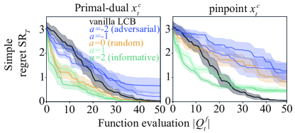
(a) (a) Primal-dual vs pinpointing

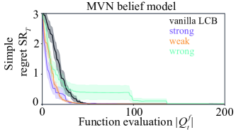
(b) (b) MVN human belief model

Figure 6: Different forms of human feedback

We demonstrate the adaptation of (a) pinpoint and (d) belief function forms in Fig. 6. The pinpoint strategy employs a sample from the expert belief function as $x_{c}$ on line 4 in Algorithm 1, while keeping the remaining lines the same as the original. It performs worse than the original primal-dual approaches, particularly in later iterations. This is because expert sampling does not incorporate GP information. Generally, humans excel at exploration in the beginning, while GP excels at finding precise locations in the later stages. This finding is supported by other literature, such as [47], involving human expert studies.

In Fig. 6(b), we employed the multivariate normal distribution (MVN) belief model proposed by [42]. This model represents the human belief function as $\tilde{p}=\mathcal{N}(x;\mu,\Sigma)$, where $\mu$ is the mean vector representing the estimated location of the global optimum $x^{*}$, and $\Sigma$ is the covariance matrix, representing the confidence of the estimation. We use $\Sigma=\textbf{I}$, the identity matrix I, as suggested by [42]. We transform: $[0,{|2\pi\Sigma|}^{-1/2}]\rightarrow[0,1]$, and we use this normalised belief function as the acceptance probability of a Bernoulli distribution $1-p$ at given location $x$ (note that $p=0$ is acceptance). Following [42], we set three levels of beliefs: strong, weak, and wrong. These levels are established by adjusting the mean vector to be offset from $x^{*}$. ‘Strong’ aligns with $x^{*}$, ‘wrong’ is the furthest possible location from $x^{*}$, and ‘weak’ is an intermediate location. Our algorithm robustly converges for any level of trust.

As such, the primary reason we adopted binary labelling is due to its empirical success, as demonstrated in Fig. 5 and Fig. 6. None of the other formats, including (a) pinpoint form [11, 49] and (b) pairwise comparison [7], outperforms our method. In the experiments by [7], the authors showed that (a) pairwise comparison outperforms both (d) belief form [42]. Therefore, it logically follows that our binary labeling format yields the best performance.

The main reasons why the binary format works better are as follows:

1. Pinpoint form: The accuracy of pinpointing is generally lower than that of kernel-based models. Humans excel at qualitative comparison rather than estimating absolute quantities [46]. Numerous studies [11, 47, 49, 69] have confirmed that manual search (pinpointing) by human experts only outperforms in the initial stages, with standard BO with GP performing better in later rounds. [38] shows that this type of feedback only outperforms when the expert’s manual sampling is consistently superior to the standard BO. However, such cases are rare in our examples (e.g., Rosenbrock), and [11, 69] corroborate this conclusion.

2. Pairwise comparison: This format relies on two critical assumptions: transitivity and completeness. Transitivity assumes no inconsistencies, which are often referred to as a "rock-paper-scissors" relationship. However, real-world human preferences frequently exhibit this issue [20]. Completeness assumes that humans can always rank their preferences at any given points. In practice, when a user is unsure which option is better, this assumption does not hold. Our imprecise probability approach avoids these issues by not relying on an absolute ranking structure [10, 40].

3. Ranking: Ranking is an extension of pairwise comparison and has been classically researched as the Borda count, which is known not to satisfy all rational axioms. Theoretically, the Condorcet winner in pairwise comparison is the only method that is known to identify the global maximum of ordinal utility.

4. Belief function: This is another form of absolute quantity, which humans are generally not proficient at estimating. Additionally, the offline nature of this method does not allow for knowledge updates.

Appendix I Potential Extensions for Future Work

I.1 Extension to Time-varying Human Feedback Model

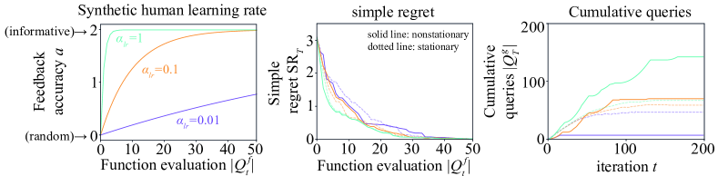
Figure 7: Non-stationary human accuracy.

In practice, human’s belief in the black-box function may be influenced by the online evaluation results of the ground-truth black-box function. To further incorporate such online influence, we need to model the change of human feedback model.

Simple extension, yet not promising performance gain. The most naïve approach for non-stationary model is windowing, i.e., forgetting the previous queried dataset. This can be very easy to apply to our setting, as it simply removes the old data outside the predefined iteration window.

Fig. 7 shows the scenario where the accuracy of human experts’ labelling improves over time, represented by $a=2(1-\exp(-\alpha_{lr}/|Q_{t}^{f}|))$, where $\alpha_{lr}$ controls the learning rate. The non-stationary model employs windowing, retaining only the most recent $w$-th data points, with $w=5$. The stationary model does not use windowing, thereby retaining all labelled datasets. The plots represent the average of 10 runs without standard error for improved visibility. While simple regret showed slight improvement initially, the performance gain varied depending on $\alpha_{lr}$. In contrast, the cumulative number of queries $|Q_{t}^{g}|$ significantly increased due to the increased uncertainty introduced by windowing.

More sophisticated extension. Another more sophisticated approach is modelling the dynamics of behavioural change. A potential idea is modelling the human behaviour change as an implicit online learning process of the latent function $g$. That is, $g_{t+1}=F(g_{t},x_{t},y_{t})$, where $g_{t}$ is the human latent function at step $t$. The forward dynamics $F$ captures the update of human latent function $g$ when observing the new data point. One potential $F$ is gradient ascent of log-likelihood as shown in $g_{t+1}=g_{t}+\lambda\nabla_{g}\log p_{g}(x_{t},y_{t})$, where $p_{g}(x_{t},y_{t})$ is the probability of observing $y_{t}$ at the input $x_{t}$ given the black-box objective function is $g$. We can then combine this dynamic with our likelihood ratio model. Since this part requires significantly different analysis and experiments, we leave it as future work.

I.2 Extension to Adaptive Trust Weight $\eta$

In line 6 of Alg. 2, the weight $\eta$ is fixed. An adaptive $\eta$ could offer better resilience to adversity. However, even without such a scheme, our no-harm guarantee holds, both theoretically and empirically.

Adaptation through the posterior standard deviation. Although $\eta$ is set to be a constant in our current design of the algorithm, there is still adaptation on trusting human or the vanilla BO algorithm through the time-varying posterior standard deviation. Intuitively, if originally the expert-augmented solution $x_{t}^{c}$ is trusted more, more samples are allocated to human-preferred region and $\sigma_{t}(x_{t}^{c})$ drops quickly. Intuitively, if we keep sampling $x_{t}^{c}$ and $x_{t}^{u}\neq x_{t}^{c}$, $\sigma_{t}(x_{t}^{u})$ would finally be larger than $\eta\sigma_{t}(x_{t}^{c})$ and we switch to sampling $x_{t}^{u}$.

Choice of $\eta$ does not need to be very large in practice. Intuitively, $\eta$ captures the belief on the expertise level of the human. The more trust we have on the expertise of the human, the larger $\eta$ we can choose. But larger $\eta$ increases the risk of higher regret due to potential over-trust in adversarial human labeler. In our experience, $\eta$ does not need to be very large. Indeed, $\eta=3$ already achieves superior performance in our experiment (see Fig. 3).

I.3 Extension to Different Acquisition Function

Our algorithm can be easily extended to other acquisition functions. For example, we can indeed use similar idea to extend expected improvement (EI) acquisition function to human constrained expected improvement (HCEI) to generate $x_{t}^{c}$.

$$x_{t}^{c}\in\arg\max_{x\in\mathcal{X}}\mathbb{P}(x\textrm{ is accepted by human})\mathrm{EI}(x).$$ (70)

Appendix J Experiments

J.1 Hyperparameters

Table 3: The complete list of hyperparameters and their settings.

hyperparameters	initial value	data-driven optimisation?	tuning method
$f$ kernel hyperparamters	BoTorch default	✓	maximising the marginal likelihood
$g$ kernel hyperparamters	BoTorch default	✓	copying $f$ kernel values
$r$ in Eq.2b	1e-4	fixed	–
$\gamma_{|\mathcal{Q}^{f}_{t}|}^{f}$ in Eq.3	–	✓	algorithm using [39]
$B_{f}$ in Lemma 3.1	standardised (=1)	fixed	–
$\sigma$ in Lemma 3.1	$\sigma=r$	fixed	–
$\delta$ in Lemma 3.1	0.01	fixed	–
$\beta_{f_{t}}$ in Lemma 3.1	1	✓	using the equation in Lemma 3.1
$\lambda_{t}$ in Eq. 6	1	✓	using dual update in Eq. 5
$\xi$ in Eq. 5	0.02	fixed	–
$B_{g}$ in Eq. 6	1	✓	the method in Appendix F
$\alpha_{1}$ in Eq. 6	0.01	✓	the method in Appendix F
$\eta$ in line. 6 in Alg. 1	3	fixed	–
$g_{\text{thr}}$ in line. 8 in Alg. 1	1e-5	fixed	–

We summarized the comprehensive list of hyperparameters used in this work and their settings in Table 3. Most of these are standard in typical GP-UCB approaches. The newly introduced hyperparameters are primarily tunable in a data-driven manner, and we provided a sensitivity analysis in the experiment section for those that are not.

J.2 Synthetic Function Details

J.2.1 Task Definitions

Ackely

Ackley funciton is defined as:

$$f(x):=-a\exp\left[-b\sqrt{\frac{1}{d}\sum_{i=1}^{d}x_{i}^{2}}\right]-\exp\left[\frac{1}{d}\sum_{i=1}^{d}\cos(cx_{i})\right]+a+\exp(1)$$ (71)

where $a=20,c=2\pi,d=4$. We take the negative Ackley function as the objective of BO to make this optimisation problem maximisation. This is a 4-dimensional function bounded by $x\in[-1,1]^{d}$. The global optimum is $x^{*}=[0,0,0,0]$ and $f(x^{*})=0$.

Hölder Table

Hölder Table funciton is defined as:

$$f(x):=\Bigg{\lvert}\sin(x_{1})\cos(x_{2})\exp\left(\Bigg{\lvert}1-\frac{\sqrt{x_{1}^{2}+x_{2}^{2}}}{\pi}\Bigg{\rvert}\right)\Bigg{\rvert}$$ (72)

where $x_{i}$ is the $i$-th dimensional input. This is a 2-dimensional function bounded by $x\in[0,10]^{d}$. The global optimum is $x^{*}=[8.05502,9.66459]$ and $f(x^{*})=19.2085$.

Rastringin

Rastringin function is defined as:

$$f(x):=10d\sum_{i=1}^{d}\left[x^{2}_{i}-10\cos(2\pi x_{i})\right]$$ (73)

where $x_{i}$ is the $i$-th dimensional input. This is a 2-dimensional function bounded by $x\in[-5.12,5.12]^{d}$. The global optimum is $x^{*}=[0,0]$ and $f(x^{*})=0$.

Michalewicz

Michalewicz funciton is defined as:

$$f(x):=\sum_{i=1}^{d}\sin(x_{i})\sin^{2m}\left(\frac{ix_{i}^{2}}{\pi}\right)$$ (74)

where $x_{i}$ is the $i$-th dimensional input and $m=10$. This is a 5-dimensional function bounded by $x\in[0,\pi]^{d}$. The global optimum is $f(x^{*})=-4.687658$.

Rosenbrock

Rosenbrock funciton is defined as:

$$f(x):=\sum_{i=1}^{d-1}\left[100(x_{i+1}-x_{i}^{2})^{2}+(x_{i}-1)^{2}\right]$$ (75)

where $x_{i}$ is the $i$-th dimensional input. This is a 3-dimensional function bounded by $x\in[-5,10]^{d}$. The global optimum is $x^{*}=[1]^{d}$ and $f(x^{*})=0$.

J.2.2 Computational time and elicitation efficiency

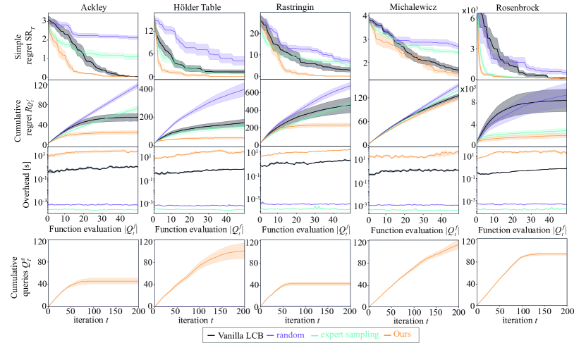
Figure 8: Simple and cumulative regrets, overhead, and cumulative queries for synthetic experiments.

Figure 8 presents the comprehensive experimental results, including overhead and cumulative queries. Overhead refers to the wall-clock time in seconds required to generate the next query location. While the time taken to query the objective function is excluded, the time to query human (or synthetic) experts is included. Our overhead is the largest among the simple baselines; however, an average of around 10 seconds per query is reasonable when compared to more computationally expensive algorithms, such as information-theoretic acquisition functions, which typically require several hours per query. In most experiments, we observe a plateau in cumulative queries, indicating a handover guarantee. In the case of the Michalewicz function, a plateau has not yet been reached due to its high-dimensional nature. Nevertheless, we observe convergence acceleration in both simple and cumulative regrets.

J.2.3 Comprehensive check for no-harm guarantee

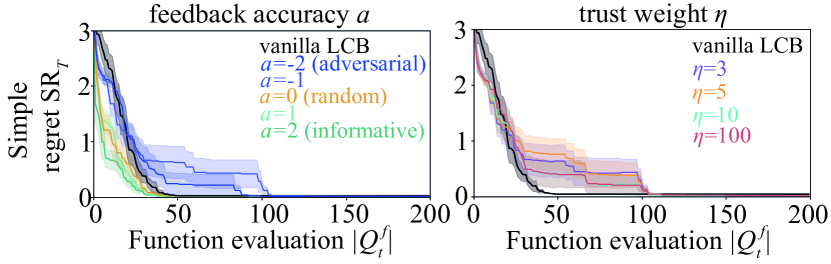
Figure 9: Confirming no-harm guarantee.

We examine the no-harm guarantee by extending the iterations to confirm that our algorithm can converge at a rate comparable to the vanilla LCB. We tested with the two adversarial cases; (1) varying feedback accuracy $a\in\{-2,-1,0,1,2\}$ for the fixed trust weight $\eta=3$ and (2) varying trust weights $\eta\in\{3,5,10,100\}$ for the fixed accuracy $a=-2$. Our algorithm converges to the same regret as the vanilla LCB over multiple iterations in both cases. We observed saturation behavior, where the convergence drop starts at similar locations among larger $\eta$, indicating that the no-harm guarantee is assured regardless of how large $\eta$ becomes. Particularly, the convergence curves of $\eta=10$ and $\eta=100$ are almost identical, supporting the saturation perspective.

J.3 Human experiment details

J.3.1 Task definitions

The task involves identifying the optimal electrolyte material combination to maximize ionic conductivity in lithium-ion batteries. Ionic conductivity is crucial for reducing internal resistance, which is essential for fast charging. Slow charging remains one of the biggest challenges for the widespread adoption of electric vehicles. Therefore, finding the best electrolyte combination is crucial to advancing electric vehicle development and realizing a sustainable society.

In our study, we considered four types of electrolyte materials. For demonstration purposes, we did not conduct physical experiments. Instead, we utilized an open dataset and fitted functions to interpolate between data points, creating a continuous search space. Experiments were then performed on this synthetic data using software and four human experts. In real-world development, researchers and engineers synthesize these materials, which is expensive, making the expert’s labeling process significantly cheaper than objective queries.

Li⁺ standard design

The first task involves the EC-DMC-EMC-LiPF₆ system [26, 7], where EC, DMC, and EMC are ethylene carbonate, dimethyl carbonate, and ethyl methyl carbonate, respectively, and LiPF₆ is lithium hexafluorophosphate. Ionic conductivity depends on both lithium salt molarity and cosolvent composition. Using the dataset from [26], we fitted the Casteel-Amis equation [19] and extended it to a continuous space. The input features are (1) LiPF₆ molarity, (2) DMC vs. EMC cosolvent ratio, and (3) EC vs. carbonates cosolvent ratio, with inputs bounded as $x_{1}\in[0,2]$, $x_{2}\in[0,1]$, and $x_{3}\in[0,1]$. The output is generated by adding i.i.d. zero-mean Gaussian noise with a variance of 1 to the noiseless function. We take the negative of the ionic conductivity in log mS/cm as the minimization objective.

Li⁺ methyl-acetate

The second task involves the MA-DMC-EMC-LiPF₆ system [55, 7], with MA being methyl acetate. Using the dataset from [55], we fitted the Casteel-Amis equation and extended it to continuous space. The input features are (1) LiPF₆ molarity, (2) DMC vs. EMC cosolvent ratio, and (3) MA vs. carbonates cosolvent ratio, with inputs bounded as $x_{1}\in[0,2]$, $x_{2}\in[0,1]$, and $x_{3}\in[0,1]$. The output is generated by adding i.i.d. zero-mean Gaussian noise with a variance of 1 to the noiseless function. We take the negative of the ionic conductivity in log mS/cm as the minimization objective.

Li⁺ polymer-nanocomposite

The third task involves the PEO-LLZTO nanocomposite electrolyte system [107], where PEO is polyethylene oxide, and LLZTO is lithium garnet (Li${}_{6}.4$La₃Zr${}_{1}.4$Ta${}_{0}.6$O${}_{1}2$) nanoparticles. Using the dataset from[107], we fitted a GP model and extended it to continuous space. The input features are (1) PEO volume %, (2) LLZTO volume %, and (3) LLZTO particle size in micrometers, with inputs bounded as $x_{1}\in[70,95]$, $x_{2}\in[5,30]$, and $x_{3}\in[0.04,10]$. The output is generated by adding i.i.d. zero-mean Gaussian noise with a variance of 1 to the noiseless function. We take the negative of the ionic conductivity in log mS/cm as the minimization objective.

Li⁺ Ionic liquid

The fourth task involves the bmimSCN-LiClO₄-LiTFSI ionic liquid [71], where bmimSCN is 1-butyl-3-methylimidazolium thiocyanate, LiClO₄ is lithium perchlorate, and LiTFSI is lithium bis(trifluoromethanesulfonyl)imide. Using the dataset from [71], we fitted a GP model and extended it to continuous space. The input features are (1) LiClO₄ molarity, (2) LiTFSI molarity, and (3) bmimSCN molarity, with inputs bounded as $x_{1}\in[0,4]$, $x_{2}\in[0,1.5]$, and $x_{3}\in[3,5]$. The output is generated by adding i.i.d. zero-mean Gaussian noise with a variance of 1 to the noiseless function. We take the negative of the ionic conductivity in log mS/cm as the minimization objective.

J.4 How Do Human Experts Reason?

We explore how experts reason through these optimization tasks. Ionic conductivity is roughly estimated by the product of movable ion density and diffusivity, as described by the Nernst-Einstein equation. Experts base their evaluations on this relationship.

Li⁺ standard design

In this system, EC plays a crucial role in both factors. LiPF₆ provides movable ions (Li⁺ and PF${}_{6}^{-}$), but these ions are not mobile in their raw state due to strong electrostatic forces. EC, a highly polarized but non-charged solvent, dissolves LiPF₆ through solvation. Increasing EC concentration can raise movable ion density, but EC’s high viscosity slows diffusivity, creating a convex curve. Experts generally agree that the global maximum is around 30% EC and 1 M LiPF₆, but the optimal EMC/DMC ratio remains uncertain. EMC and DMC are similar, with EMC being larger and asymmetric, and DMC being smaller and symmetric. Smaller molecules tend to be more diffusive, so a higher DMC ratio is expected to be better, although the asymmetric structure of EMC could disrupt higher-order solvation networks, contributing to diffusivity.

In summary, experts vaguely know the whole function shape and possible global optimum location for two variables, yet others are unknown.

Li⁺ methyl-acetate

his task involves replacing EC with MA from the first task, making the overall system similar. However, MA is an unusual material, and none of the participants are familiar with it. We will explain how experts reasoned this change in the optimization task.

EC plays a central role in dissolving LiPF₆, increasing movable ion density, although it is viscous. While no one knows methyl acetate, it can be inferred that it also dissolves LiPF₆. The challenge lies in determining its polarization ability and viscosity. EC is a planar molecule with a five-membered ring, resembling a ‘small sheet magnet’ with strong magnetic power but easy stacking. Conversely, MA is a small, non-ring-structured, asymmetric molecule. This asymmetry prevents MA molecules from stacking, enhancing diffusivity. However, the asymmetry also reduces polarization, leading to a weaker solvation effect and lower movable ion density.

Thus, MA has a mix of positive and negative effects, making it difficult for experts to predict the exact shape of the convex curve. Nonetheless, in most "less viscous" solvent systems, the peak typically occurs around 1.5 M of LiPF₆. Experts can roughly estimate this position, and this estimation is fairly accurate, as the true position is at 1.35 M.

Li⁺ polymer-nanocomposite

This task is completely different from the previous two tasks. Our electrolyte is now solid-state rather than liquid, so the Nernst-Einstein equation may not be applicable. However, the core idea remains the same. PEO is a framework material without ionic conductivity, whereas LLZTO has ionic conductivity. Generally, a higher LLZTO content should result in greater conductivity. Other factors are less certain.

We can anticipate the effects in both directions. Smaller particle sizes might be better because they distribute more evenly within the PEO, increasing ionic conductive paths. However, smaller particles might also be worse due to increased grain boundaries and aggregation caused by electric forces. Thus, most experts expected a convex relationship with particle size and a monotonic increase with LLZTO ratio.

In reality, experimental results showed that conductivity improved monotonically with smaller particle sizes and displayed a convex relationship with LLZTO volume. Therefore, the experts’ advice was somewhat inaccurate.

Looking back, experts were partially correct. Aggregation did create the convex shape in LLZTO volume ratio, indicating their understanding of the phenomenon. However, they did not identify the correct input dimension where aggregation mattered. For particle size, the thorough mixing procedure with ball milling used in the dataset prevented aggregation, leading to misconceptions about the function shape.

Na⁺ Ionic liquid

This task is completely different from the previous tasks. Although our electrolyte is liquid, all materials are ionically conductive. As the name suggests, ionic liquids are special materials that can dissolve themselves without the need for a cosolvent. Consequently, the movable ion density factor remains almost unchanged, as all components are conductive regardless of composition. Therefore, diffusivity becomes the dominant factor. Diffusivity primarily depends on two factors: molecule size and electric interaction. Smaller molecules are generally more mobile, but they also have stronger electric interactions when the charge is the same (all ions in this system are monovalent).

This dual dependence leads to different expectations: if size is the dominant factor, smaller molecules (like LiCl₄) are expected to perform best. Conversely, if electric interaction is dominant, the results will differ.

Most experts anticipated a monotonic change in all dimensions, expecting both LiCl₄ and LiTFSI to show increased performance due to their smaller size compared to bmimSCN. However, experimental results showed a double peak shape for LiTFSI vs. bmimSCN and a convex shape for LiCl₄ and bmimSCN. Thus, the experts’ advice was inaccurate. The real physical phenomena were more complex than initially thought, with electric interactions playing a more dominant role.

J.4.1 Computational time and elicitation efficiency

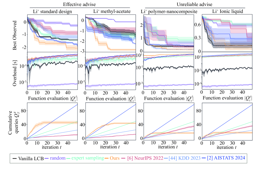
Figure 10: Simple and cumulative regrets, overhead, and cumulative queries for real-world experiments.

Figure 10 illustrates the full experimental results, including the best observed values $\max Y_{|\mathcal{Q}^{f}_{T}|}$, overhead, and cumulative queries $\mathcal{Q}^{g}_{t}$. The overhead definition remains consistent with that in the synthetic experiments. Note that these experiments include only four human trials, resulting in noisier data compared to the synthetic experiments, which used 10 random seeds. The overhead for our method and the baselines is approximately the same, around 10 seconds per query. This is manageable compared to the significantly slower methods, such as information-theoretic acquisition functions, which take several hours per query.

Regarding cumulative queries, only our method demonstrates a handover guarantee. While baseline methods continue to request human intervention even as the experiments conclude, our method stops requesting input midway through the experiments, thereby freeing the human expert from the task. Our approach allows for more effective input from experts in cases where their advice is beneficial and reduces input in unreliable cases. In contrast, the baselines request input regardless of the quality of the advice. Notably, the method described in [11] increases the frequency of requests when experts provide incorrect information. This occurs because disagreements between the surrogate $f$ and human beliefs prompt human experts to intervene, aiming to prevent the BO from proceeding in the wrong direction. Unfortunately, this intervention can act as an adversarial response. In contrast, our algorithm avoids such scenarios through active learning constraints (as highlighted in line 6), thus achieving a no-harm guarantee in unreliable cases.

NeurIPS Paper Checklist

1. Claims

2. Question: Do the main claims made in the abstract and introduction accurately reflect the paper’s contributions and scope?

3. Answer: [Yes]

4. Justification: Elicitation efficiency and no-harm guarantee are proved in Theorem 4.1. Experiments shows empirical efficacy in Figures 3, 4, 5, 8, 10.

5. Guidelines:

   • The answer NA means that the abstract and introduction do not include the claims made in the paper.

   • The abstract and/or introduction should clearly state the claims made, including the contributions made in the paper and important assumptions and limitations. A No or NA answer to this question will not be perceived well by the reviewers.

   • The claims made should match theoretical and experimental results, and reflect how much the results can be expected to generalize to other settings.

   • It is fine to include aspirational goals as motivation as long as it is clear that these goals are not attained by the paper.

6. Limitations

7. Question: Does the paper discuss the limitations of the work performed by the authors?

8. Answer: [Yes]

9. Justification: See Conclusion and Limitation section.

10. Guidelines:

    • The answer NA means that the paper has no limitation while the answer No means that the paper has limitations, but those are not discussed in the paper.

    • The authors are encouraged to create a separate "Limitations" section in their paper.

    • The paper should point out any strong assumptions and how robust the results are to violations of these assumptions (e.g., independence assumptions, noiseless settings, model well-specification, asymptotic approximations only holding locally). The authors should reflect on how these assumptions might be violated in practice and what the implications would be.

    • The authors should reflect on the scope of the claims made, e.g., if the approach was only tested on a few datasets or with a few runs. In general, empirical results often depend on implicit assumptions, which should be articulated.

    • The authors should reflect on the factors that influence the performance of the approach. For example, a facial recognition algorithm may perform poorly when image resolution is low or images are taken in low lighting. Or a speech-to-text system might not be used reliably to provide closed captions for online lectures because it fails to handle technical jargon.

    • The authors should discuss the computational efficiency of the proposed algorithms and how they scale with dataset size.

    • If applicable, the authors should discuss possible limitations of their approach to address problems of privacy and fairness.

    • While the authors might fear that complete honesty about limitations might be used by reviewers as grounds for rejection, a worse outcome might be that reviewers discover limitations that aren’t acknowledged in the paper. The authors should use their best judgment and recognize that individual actions in favor of transparency play an important role in developing norms that preserve the integrity of the community. Reviewers will be specifically instructed to not penalize honesty concerning limitations.

11. Theory Assumptions and Proofs

12. Question: For each theoretical result, does the paper provide the full set of assumptions and a complete (and correct) proof?

13. Answer: [Yes]

14. Justification: Assumptions 2.1-2.6, Proofs in Appendices A-C.

15. Guidelines:

    • The answer NA means that the paper does not include theoretical results.

    • All the theorems, formulas, and proofs in the paper should be numbered and cross-referenced.

    • All assumptions should be clearly stated or referenced in the statement of any theorems.

    • The proofs can either appear in the main paper or the supplemental material, but if they appear in the supplemental material, the authors are encouraged to provide a short proof sketch to provide intuition.

    • Inversely, any informal proof provided in the core of the paper should be complemented by formal proofs provided in appendix or supplemental material.

    • Theorems and Lemmas that the proof relies upon should be properly referenced.

16. Experimental Result Reproducibility

17. Question: Does the paper fully disclose all the information needed to reproduce the main experimental results of the paper to the extent that it affects the main claims and/or conclusions of the paper (regardless of whether the code and data are provided or not)?

18. Answer: [Yes]

19. Justification: Experimental section, Appendix J, open-sourced code (anonymous) https://github.com/ma921/COBOL/

20. Guidelines:

    • The answer NA means that the paper does not include experiments.

    • If the paper includes experiments, a No answer to this question will not be perceived well by the reviewers: Making the paper reproducible is important, regardless of whether the code and data are provided or not.

    • If the contribution is a dataset and/or model, the authors should describe the steps taken to make their results reproducible or verifiable.

    • Depending on the contribution, reproducibility can be accomplished in various ways. For example, if the contribution is a novel architecture, describing the architecture fully might suffice, or if the contribution is a specific model and empirical evaluation, it may be necessary to either make it possible for others to replicate the model with the same dataset, or provide access to the model. In general. releasing code and data is often one good way to accomplish this, but reproducibility can also be provided via detailed instructions for how to replicate the results, access to a hosted model (e.g., in the case of a large language model), releasing of a model checkpoint, or other means that are appropriate to the research performed.

    • While NeurIPS does not require releasing code, the conference does require all submissions to provide some reasonable avenue for reproducibility, which may depend on the nature of the contribution. For example

      1. If the contribution is primarily a new algorithm, the paper should make it clear how to reproduce that algorithm.

      2. If the contribution is primarily a new model architecture, the paper should describe the architecture clearly and fully.

      3. If the contribution is a new model (e.g., a large language model), then there should either be a way to access this model for reproducing the results or a way to reproduce the model (e.g., with an open-source dataset or instructions for how to construct the dataset).

      4. We recognize that reproducibility may be tricky in some cases, in which case authors are welcome to describe the particular way they provide for reproducibility. In the case of closed-source models, it may be that access to the model is limited in some way (e.g., to registered users), but it should be possible for other researchers to have some path to reproducing or verifying the results.

21. Open access to data and code

22. Question: Does the paper provide open access to the data and code, with sufficient instructions to faithfully reproduce the main experimental results, as described in supplemental material?

23. Answer: [Yes]

24. Justification: Provide data and code on Anonymised repository https://github.com/ma921/COBOL/

25. Guidelines:

    • The answer NA means that paper does not include experiments requiring code.

    • Please see the NeurIPS code and data submission guidelines (https://nips.cc/public/guides/CodeSubmissionPolicy) for more details.

    • While we encourage the release of code and data, we understand that this might not be possible, so “No” is an acceptable answer. Papers cannot be rejected simply for not including code, unless this is central to the contribution (e.g., for a new open-source benchmark).

    • The instructions should contain the exact command and environment needed to run to reproduce the results. See the NeurIPS code and data submission guidelines (https://nips.cc/public/guides/CodeSubmissionPolicy) for more details.

    • The authors should provide instructions on data access and preparation, including how to access the raw data, preprocessed data, intermediate data, and generated data, etc.

    • The authors should provide scripts to reproduce all experimental results for the new proposed method and baselines. If only a subset of experiments are reproducible, they should state which ones are omitted from the script and why.

    • At submission time, to preserve anonymity, the authors should release anonymized versions (if applicable).

    • Providing as much information as possible in supplemental material (appended to the paper) is recommended, but including URLs to data and code is permitted.

26. Experimental Setting/Details

27. Question: Does the paper specify all the training and test details (e.g., data splits, hyperparameters, how they were chosen, type of optimizer, etc.) necessary to understand the results?

28. Answer: [Yes]

29. Justification: See experimental section and Appendix J.

30. Guidelines:

    • The answer NA means that the paper does not include experiments.

    • The experimental setting should be presented in the core of the paper to a level of detail that is necessary to appreciate the results and make sense of them.

    • The full details can be provided either with the code, in appendix, or as supplemental material.

31. Experiment Statistical Significance

32. Question: Does the paper report error bars suitably and correctly defined or other appropriate information about the statistical significance of the experiments?

33. Answer: [Yes]

34. Justification: All experiments report the $\pm$ standard errors.

35. Guidelines:

    • The answer NA means that the paper does not include experiments.

    • The authors should answer "Yes" if the results are accompanied by error bars, confidence intervals, or statistical significance tests, at least for the experiments that support the main claims of the paper.

    • The factors of variability that the error bars are capturing should be clearly stated (for example, train/test split, initialization, random drawing of some parameter, or overall run with given experimental conditions).

    • The method for calculating the error bars should be explained (closed form formula, call to a library function, bootstrap, etc.)

    • The assumptions made should be given (e.g., Normally distributed errors).

    • It should be clear whether the error bar is the standard deviation or the standard error of the mean.

    • It is OK to report 1-sigma error bars, but one should state it. The authors should preferably report a 2-sigma error bar than state that they have a 96% CI, if the hypothesis of Normality of errors is not verified.

    • For asymmetric distributions, the authors should be careful not to show in tables or figures symmetric error bars that would yield results that are out of range (e.g. negative error rates).

    • If error bars are reported in tables or plots, The authors should explain in the text how they were calculated and reference the corresponding figures or tables in the text.

36. Experiments Compute Resources

37. Question: For each experiment, does the paper provide sufficient information on the computer resources (type of compute workers, memory, time of execution) needed to reproduce the experiments?

38. Answer: [Yes]

39. Justification: See experimental section and footnote 2. See also Appendix J.

40. Guidelines:

    • The answer NA means that the paper does not include experiments.

    • The paper should indicate the type of compute workers CPU or GPU, internal cluster, or cloud provider, including relevant memory and storage.

    • The paper should provide the amount of compute required for each of the individual experimental runs as well as estimate the total compute.

    • The paper should disclose whether the full research project required more compute than the experiments reported in the paper (e.g., preliminary or failed experiments that didn’t make it into the paper).

41. Code Of Ethics

42. Question: Does the research conducted in the paper conform, in every respect, with the NeurIPS Code of Ethics https://neurips.cc/public/EthicsGuidelines?

43. Answer: [Yes]

44. Justification: Our research is pure algorithm development.

45. Guidelines:

    • The answer NA means that the authors have not reviewed the NeurIPS Code of Ethics.

    • If the authors answer No, they should explain the special circumstances that require a deviation from the Code of Ethics.

    • The authors should make sure to preserve anonymity (e.g., if there is a special consideration due to laws or regulations in their jurisdiction).

46. Broader Impacts

47. Question: Does the paper discuss both potential positive societal impacts and negative societal impacts of the work performed?

48. Answer: [Yes]

49. Justification: See Conclusion and Limitation.

50. Guidelines:

    • The answer NA means that there is no societal impact of the work performed.

    • If the authors answer NA or No, they should explain why their work has no societal impact or why the paper does not address societal impact.

    • Examples of negative societal impacts include potential malicious or unintended uses (e.g., disinformation, generating fake profiles, surveillance), fairness considerations (e.g., deployment of technologies that could make decisions that unfairly impact specific groups), privacy considerations, and security considerations.

    • The conference expects that many papers will be foundational research and not tied to particular applications, let alone deployments. However, if there is a direct path to any negative applications, the authors should point it out. For example, it is legitimate to point out that an improvement in the quality of generative models could be used to generate deepfakes for disinformation. On the other hand, it is not needed to point out that a generic algorithm for optimizing neural networks could enable people to train models that generate Deepfakes faster.

    • The authors should consider possible harms that could arise when the technology is being used as intended and functioning correctly, harms that could arise when the technology is being used as intended but gives incorrect results, and harms following from (intentional or unintentional) misuse of the technology.

    • If there are negative societal impacts, the authors could also discuss possible mitigation strategies (e.g., gated release of models, providing defenses in addition to attacks, mechanisms for monitoring misuse, mechanisms to monitor how a system learns from feedback over time, improving the efficiency and accessibility of ML).

51. Safeguards

52. Question: Does the paper describe safeguards that have been put in place for responsible release of data or models that have a high risk for misuse (e.g., pretrained language models, image generators, or scraped datasets)?

53. Answer: [N/A] .

54. Justification: Our paper is a pure algorithm study for blackbox optimization for small, lower dimensional tasks.

55. Guidelines:

    • The answer NA means that the paper poses no such risks.

    • Released models that have a high risk for misuse or dual-use should be released with necessary safeguards to allow for controlled use of the model, for example by requiring that users adhere to usage guidelines or restrictions to access the model or implementing safety filters.

    • Datasets that have been scraped from the Internet could pose safety risks. The authors should describe how they avoided releasing unsafe images.

    • We recognize that providing effective safeguards is challenging, and many papers do not require this, but we encourage authors to take this into account and make a best faith effort.

56. Licenses for existing assets

57. Question: Are the creators or original owners of assets (e.g., code, data, models), used in the paper, properly credited and are the license and terms of use explicitly mentioned and properly respected?

58. Answer: [Yes]

59. Justification: See experimental section.

60. Guidelines:

    • The answer NA means that the paper does not use existing assets.

    • The authors should cite the original paper that produced the code package or dataset.

    • The authors should state which version of the asset is used and, if possible, include a URL.

    • The name of the license (e.g., CC-BY 4.0) should be included for each asset.

    • For scraped data from a particular source (e.g., website), the copyright and terms of service of that source should be provided.

    • If assets are released, the license, copyright information, and terms of use in the package should be provided. For popular datasets, paperswithcode.com/datasets has curated licenses for some datasets. Their licensing guide can help determine the license of a dataset.

    • For existing datasets that are re-packaged, both the original license and the license of the derived asset (if it has changed) should be provided.

    • If this information is not available online, the authors are encouraged to reach out to the asset’s creators.

61. New Assets

62. Question: Are new assets introduced in the paper well documented and is the documentation provided alongside the assets?

63. Answer: [Yes]

64. Justification: Documents are available on Anonymised repository https://anonymous.4open.science/r/COBOL-9B8B/

65. Guidelines:

    • The answer NA means that the paper does not release new assets.

    • Researchers should communicate the details of the dataset/code/model as part of their submissions via structured templates. This includes details about training, license, limitations, etc.

    • The paper should discuss whether and how consent was obtained from people whose asset is used.

    • At submission time, remember to anonymize your assets (if applicable). You can either create an anonymized URL or include an anonymized zip file.

66. Crowdsourcing and Research with Human Subjects

67. Question: For crowdsourcing experiments and research with human subjects, does the paper include the full text of instructions given to participants and screenshots, if applicable, as well as details about compensation (if any)?

68. Answer: [Yes]

69. Justification: See experimental section and Appendix J.

70. Guidelines:

    • The answer NA means that the paper does not involve crowdsourcing nor research with human subjects.

    • Including this information in the supplemental material is fine, but if the main contribution of the paper involves human subjects, then as much detail as possible should be included in the main paper.

    • According to the NeurIPS Code of Ethics, workers involved in data collection, curation, or other labor should be paid at least the minimum wage in the country of the data collector.

71. Institutional Review Board (IRB) Approvals or Equivalent for Research with Human Subjects

72. Question: Does the paper describe potential risks incurred by study participants, whether such risks were disclosed to the subjects, and whether Institutional Review Board (IRB) approvals (or an equivalent approval/review based on the requirements of your country or institution) were obtained?

73. Answer: [Yes]

74. Justification: While we do not have IRB approval, our institution has reviewed and approved our study as low-risk followed by the protocol indicated in https://researchsupport.admin.ox.ac.uk/governance/ethics/apply, considering that all experiments involve running software on open-source datasets. According to the NeurIPS 2024 ethics guidelines, adherence to existing protocols at the authors’ institution is required, with IRB approval being just one form of such protocols. Our institution follows its own policy, and we adhered to the standard procedure.

75. Guidelines:

    • The answer NA means that the paper does not involve crowdsourcing nor research with human subjects.

    • Depending on the country in which research is conducted, IRB approval (or equivalent) may be required for any human subjects research. If you obtained IRB approval, you should clearly state this in the paper.

    • We recognize that the procedures for this may vary significantly between institutions and locations, and we expect authors to adhere to the NeurIPS Code of Ethics and the guidelines for their institution.

    • For initial submissions, do not include any information that would break anonymity (if applicable), such as the institution conducting the review.

References

- [1] David Ackley. A connectionist machine for genetic hillclimbing, volume 28. Springer science & business media, 1987.
- [2] Masaki Adachi. High-dimensional discrete Bayesian optimization with self-supervised representation learning for data-efficient materials exploration. In NeurIPS 2021 AI for Science Workshop, 2021.
- [3] Masaki Adachi, Satoshi Hayakawa, Martin Jørgensen, Saad Hamid, Harald Oberhauser, and Michael A Osborne. A quadrature approach for general-purpose batch Bayesian optimization via probabilistic lifting. arXiv preprint arXiv:2404.12219, 2024.
- [4] Masaki Adachi, Satoshi Hayakawa, Martin Jørgensen, Harald Oberhauser, and Michael A Osborne. Fast Bayesian inference with batch Bayesian quadrature via kernel recombination. Advances in Neural Information Processing Systems (NeurIPS), 35:16533–16547, 2022.
- [5] Masaki Adachi, Satoshi Hayakawa, Martin Jørgensen, Xingchen Wan, Vu Nguyen, Harald Oberhauser, and Michael A Osborne. Adaptive batch sizes for active learning: A probabilistic numerics approach. In International Conference on Artificial Intelligence and Statistics (AISTATS), pages 496–504. PMLR, 2024.
- [6] Masaki Adachi, Yannick Kuhn, Birger Horstmann, Arnulf Latz, Michael A Osborne, and David A Howey. Bayesian model selection of lithium-ion battery models via Bayesian quadrature. IFAC-PapersOnLine, 56(2):10521–10526, 2023.
- [7] Masaki Adachi, Brady Planden, David A Howey, Michael A Osborne, Sebastian Orbell, Natalia Ares, Krikamol Muandet, and Siu Lun Chau. Looping in the human: Collaborative and explainable Bayesian optimization. In International Conference on Artificial Intelligence and Statistics (AISTATS), 2024.
- [8] Joel A E Andersson, Joris Gillis, Greg Horn, James B Rawlings, and Moritz Diehl. CasADi – A software framework for nonlinear optimization and optimal control. Mathematical Programming Computation, 11(1):1–36, 2019.
- [9] Raul Astudillo, Zhiyuan Jerry Lin, Eytan Bakshy, and Peter Frazier. qEUBO: A decision-theoretic acquisition function for preferential Bayesian optimization. In International Conference on Artificial Intelligence and Statistics (AISTATS), pages 1093–1114. PMLR, 2023.
- [10] Thomas Augustin, Frank PA Coolen, Gert De Cooman, and Matthias CM Troffaes. Introduction to imprecise probabilities, volume 591. John Wiley & Sons, 2014.
- [11] Arun Kumar AV, Santu Rana, Alistair Shilton, and Svetha Venkatesh. Human-AI collaborative Bayesian Optimisation. Advances in Neural Information Processing Systems (NeurIPS), 35:16233–16245, 2022.
- [12] Arun Kumar AV, Alistair Shilton, Sunil Gupta, Santu Rana, Stewart Greenhill, and Svetha Venkatesh. Enhanced Bayesian optimization via preferential modeling of abstract properties. arXiv preprint arXiv:2402.17343, 2024.
- [13] Hasan Bakhshi, Jonathan Downing, Michael Osborne, and Philippe Schneider. The future of skills: Employment in 2030. Pearson, 2017.
- [14] Maximilian Balandat, Brian Karrer, Daniel Jiang, Samuel Daulton, Ben Letham, Andrew G Wilson, and Eytan Bakshy. BoTorch: a framework for efficient Monte-Carlo Bayesian optimization. Advances in Neural Information Processing Systems (NeurIPS), 33:21524–21538, 2020.
- [15] Alessio Benavoli, Dario Azzimonti, and Dario Piga. Learning choice functions with Gaussian processes. In Uncertainty in Artificial Intelligence (UAI), pages 141–151. PMLR, 2023.
- [16] Rishi Bommasani, Drew A Hudson, Ehsan Adeli, Russ Altman, Simran Arora, Sydney von Arx, Michael S Bernstein, Jeannette Bohg, Antoine Bosselut, Emma Brunskill, et al. On the opportunities and risks of foundation models. arXiv preprint arXiv:2108.07258, 2021.
- [17] Ralph Allan Bradley and Milton E Terry. Rank analysis of incomplete block designs: I. the method of paired comparisons. Biometrika, 39(3/4):324–345, 1952.
- [18] Adam D Bull. Convergence rates of efficient global optimization algorithms. Journal of Machine Learning Research (JMLR), 12(10), 2011.
- [19] Jerry F Casteel and Edward S Amis. Specific conductance of concentrated solutions of magnesium salts in water-ethanol system. Journal of Chemical and Engineering Data, 17(1):55–59, 1972.
- [20] Siu Lun Chau, Javier Gonzalez, and Dino Sejdinovic. Learning inconsistent preferences with Gaussian processes. In International Conference on Artificial Intelligence and Statistics (AISTATS), pages 2266–2281. PMLR, 2022.
- [21] Yutian Chen, Xingyou Song, Chansoo Lee, Zi Wang, Richard Zhang, David Dohan, Kazuya Kawakami, Greg Kochanski, Arnaud Doucet, Marc’aurelio Ranzato, et al. Towards learning universal hyperparameter optimizers with transformers. Advances in Neural Information Processing Systems (NeurIPS), 35:32053–32068, 2022.
- [22] Sayak Ray Chowdhury and Aditya Gopalan. On kernelized multi-armed bandits. In International Conference on Machine Learning (ICML), pages 844–853. PMLR, 2017.
- [23] Wei Chu and Zoubin Ghahramani. Preference learning with Gaussian processes. In Proceedings of the 22nd international conference on Machine learning, pages 137–144, 2005.
- [24] Abdoulatif Cisse, Xenophon Evangelopoulos, Sam Carruthers, Vladimir V Gusev, and Andrew I Cooper. HypBO: Expert-guided chemist-in-the-loop Bayesian search for new materials. arXiv preprint arXiv:2308.11787, 2023.
- [25] Bo Dai, Hanjun Dai, Niao He, Weiyang Liu, Zhen Liu, Jianshu Chen, Lin Xiao, and Le Song. Coupled variational Bayes via optimization embedding. Advances in Neural Information Processing Systems (NeurIPS), 31, 2018.
- [26] Adarsh Dave, Jared Mitchell, Sven Burke, Hongyi Lin, Jay Whitacre, and Venkatasubramanian Viswanathan. Autonomous optimization of non-aqueous Li-ion battery electrolytes via robotic experimentation and machine learning coupling. Nature communications, 13(1):5454, 2022.
- [27] Nicolas Emmenegger, Mojmir Mutny, and Andreas Krause. Likelihood ratio confidence sets for sequential decision making. In Thirty-seventh Conference on Neural Information Processing Systems, 2023.
- [28] Brochu Eric, Nando Freitas, and Abhijeet Ghosh. Active preference learning with discrete choice data. In Advances in Neural Information Processing Systems (NeurIPS), volume 20, 2007.
- [29] Matthias Feurer, Aaron Klein, Katharina Eggensperger, Jost Springenberg, Manuel Blum, and Frank Hutter. Efficient and robust automated machine learning. Advances in Neural Information Processing Systems (NeurIPS), 28, 2015.
- [30] Matthias Feurer, Benjamin Letham, and Eytan Bakshy. Scalable meta-learning for Bayesian optimization using ranking-weighted Gaussian process ensembles. In AutoML Workshop at ICML, volume 7, page 5, 2018.
- [31] Jacob Gardner, Geoff Pleiss, Kilian Q Weinberger, David Bindel, and Andrew G Wilson. GPyTorch: Blackbox matrix-matrix Gaussian process inference with GPU acceleration. In Advances in Neural Information Processing Systems (NeurIPS), pages 7576–7586, 2018.
- [32] Jacob R Gardner, Matt J Kusner, Zhixiang Eddie Xu, Kilian Q Weinberger, and John P Cunningham. Bayesian optimization with inequality constraints. In International Conference on Machine Learning (ICML), volume 2014, pages 937–945, 2014.
- [33] Roman Garnett. Bayesian optimization. Cambridge University Press, 2023.
- [34] Paul H Garthwaite, Joseph B Kadane, and Anthony O’Hagan. Statistical methods for eliciting probability distributions. Journal of the American Statistical Association, 100(470):680–701, 2005.
- [35] Kevin L Gering. Prediction of electrolyte conductivity: results from a generalized molecular model based on ion solvation and a chemical physics framework. Electrochimica Acta, 225:175–189, 2017.
- [36] Javier González, Zhenwen Dai, Andreas Damianou, and Neil D Lawrence. Preferential Bayesian optimization. In International Conference on Machine Learning (ICML), pages 1282–1291. PMLR, 2017.
- [37] Shengbo Guo, Scott Sanner, and Edwin V Bonilla. Gaussian process preference elicitation. Advances in Neural Information Processing Systems (NeurIPS), 23, 2010.
- [38] Sunil Gupta, Alistair Shilton, Arun Kumar AV, Shannon Ryan, Majid Abdolshah, Hung Le, Santu Rana, Julian Berk, Mahad Rashid, and Svetha Venkatesh. BO-Muse: A human expert and AI teaming framework for accelerated experimental design. arXiv preprint arXiv:2303.01684, 2023.
- [39] Kihyuk Hong, Yuhang Li, and Ambuj Tewari. An optimization-based algorithm for non-stationary kernel bandits without prior knowledge. In International Conference on Artificial Intelligence and Statistics (AISTATS), pages 3048–3085. PMLR, 2023.
- [40] Eyke Hüllermeier and Willem Waegeman. Aleatoric and epistemic uncertainty in machine learning: An introduction to concepts and methods. Machine learning, 110(3):457–506, 2021.
- [41] Carl Hvarfner, Frank Hutter, and Luigi Nardi. A general framework for user-guided Bayesian optimization. In International Conference on Learning Representations (ICLR), 2024.
- [42] Carl Hvarfner, Danny Stoll, Artur Souza, Marius Lindauer, Frank Hutter, and Luigi Nardi. BO: Augmenting acquisition functions with user beliefs for Bayesian optimization. In International Conference on Learning Representations (ICLR), 2022.
- [43] Cole Jetton, Matthew Campbell, and Christopher Hoyle. Constraining the feasible design space in Bayesian optimization with user feedback. Journal of Mechanical Design, 146(4):041703, 2023.
- [44] Zhengbao Jiang, Frank F Xu, Jun Araki, and Graham Neubig. How can we know what language models know? Transactions of the Association for Computational Linguistics, 8:423–438, 2020.
- [45] Michael I Jordan. Artificial intelligence—the revolution hasn’t happened yet. Harvard Data Science Review, 1(1):1–9, 2019.
- [46] Daniel Kahneman and Amos Tversky. On the interpretation of intuitive probability: A reply to Jonathan Cohen. Cognition, 7(4):409–411, 1979.
- [47] Keren J Kanarik, Wojciech T Osowiecki, Yu Lu, Dipongkar Talukder, Niklas Roschewsky, Sae Na Park, Mattan Kamon, David M Fried, and Richard A Gottscho. Human–machine collaboration for improving semiconductor process development. Nature, 616(7958):707–711, 2023.
- [48] Kirthevasan Kandasamy, Jeff Schneider, and Barnabás Póczos. High dimensional Bayesian optimisation and bandits via additive models. In International Conference on Machine Learning (ICML), pages 295–304. PMLR, 2015.
- [49] Ali Khoshvishkaie, Petrus Mikkola, Pierre-Alexandre Murena, and Samuel Kaski. Cooperative Bayesian optimization for imperfect agents. In Joint European Conference on Machine Learning and Knowledge Discovery in Databases (ECML), pages 475–490. Springer, 2023.
- [50] Johannes Kirschner, Mojmir Mutny, Nicole Hiller, Rasmus Ischebeck, and Andreas Krause. Adaptive and safe Bayesian optimization in high dimensions via one-dimensional subspaces. In International Conference on Machine Learning (ICML), pages 3429–3438. PMLR, 2019.
- [51] Cheng Li, Sunil Gupta, Santu Rana, Vu Nguyen, Antonio Robles-Kelly, and Svetha Venkatesh. Incorporating expert prior knowledge into experimental design via posterior sampling. arXiv preprint arXiv:2002.11256, 2020.
- [52] Dong C Liu and Jorge Nocedal. On the limited memory BFGS method for large scale optimization. Mathematical programming, 45(1-3):503–528, 1989.
- [53] Qinghua Liu, Praneeth Netrapalli, Csaba Szepesvari, and Chi Jin. Optimistic MLE: A generic model-based algorithm for partially observable sequential decision making. In Proceedings of the 55th Annual ACM Symposium on Theory of Computing, pages 363–376, 2023.
- [54] Tennison Liu, Nicolás Astorga, Nabeel Seedat, and Mihaela van der Schaar. Large language models to enhance Bayesian optimization. In The Twelfth International Conference on Learning Representations, 2024.
- [55] ER Logan, Erin M Tonita, KL Gering, Jing Li, Xiaowei Ma, LY Beaulieu, and JR Dahn. A study of the physical properties of Li-ion battery electrolytes containing esters. Journal of The Electrochemical Society, 165(2):A21, 2018.
- [56] Arpan Losalka and Jonathan Scarlett. No-regret algorithms for safe Bayesian optimization with monotonicity constraints. In Sanjoy Dasgupta, Stephan Mandt, and Yingzhen Li, editors, Proceedings of The 27th International Conference on Artificial Intelligence and Statistics, volume 238 of Proceedings of Machine Learning Research, pages 3232–3240. PMLR, 02–04 May 2024.
- [57] Petrus Mikkola, Osvaldo A Martin, Suyog Chandramouli, Marcelo Hartmann, Oriol Abril Pla, Owen Thomas, Henri Pesonen, Jukka Corander, Aki Vehtari, Samuel Kaski, et al. Prior knowledge elicitation: The past, present, and future. arXiv preprint arXiv:2112.01380, 2112, 2021.
- [58] Petrus Mikkola, Milica Todorović, Jari Järvi, Patrick Rinke, and Samuel Kaski. Projective preferential Bayesian optimization. In International Conference on Machine Learning (ICML), pages 6884–6892. PMLR, 2020.
- [59] Jonas Mockus, Vytautas Tiesis, and Antanas Zilinskas. The application of Bayesian methods for seeking the extremum. Towards global optimization, 2(117-129):2, 1978.
- [60] Hossein Mohammadi, Rodolphe Le Riche, Nicolas Durrande, Eric Touboul, and Xavier Bay. An analytic comparison of regularization methods for Gaussian processes. arXiv preprint arXiv:1602.00853, 2016.
- [61] Quoc Phong Nguyen, Wan Theng Ruth Chew, Le Song, Bryan Kian Hsiang Low, and Patrick Jaillet. Optimistic Bayesian optimization with unknown constraints. In The Twelfth International Conference on Learning Representations, 2024.
- [62] Hannes Nickisch and Carl Edward Rasmussen. Approximations for binary Gaussian process classification. Journal of Machine Learning Research (JMLR), 9(Oct):2035–2078, 2008.
- [63] Jorge Nocedal and Stephen J Wright. Numerical optimization. Springer, 1999.
- [64] Michael A Osborne, Roman Garnett, and Stephen J Roberts. Gaussian processes for global optimization. In International Conference on Learning and Intelligent Optimization (LION3), 2009.
- [65] Long Ouyang, Jeffrey Wu, Xu Jiang, Diogo Almeida, Carroll Wainwright, Pamela Mishkin, Chong Zhang, Sandhini Agarwal, Katarina Slama, Alex Ray, John Schulman, Jacob Hilton, Fraser Kelton, Luke Miller, Maddie Simens, Amanda Askell, Peter Welinder, Paul F Christiano, Jan Leike, and Ryan Lowe. Training language models to follow instructions with human feedback. In S. Koyejo, S. Mohamed, A. Agarwal, D. Belgrave, K. Cho, and A. Oh, editors, Advances in Neural Information Processing Systems (NeurIPS), volume 35, pages 27730–27744, 2022.
- [66] Art Owen. Empirical likelihood ratio confidence regions. The Annals of Statistics, 18(1):90–120, 1990.
- [67] Anthony O’Hagan. Expert knowledge elicitation: subjective but scientific. The American Statistician, 73(sup1):69–81, 2019.
- [68] Anil Ramachandran, Sunil Gupta, Santu Rana, Cheng Li, and Svetha Venkatesh. Incorporating expert prior in Bayesian optimisation via space warping. Knowledge-Based Systems, 195:105663, 2020.
- [69] Julian Rodemann, Federico Croppi, Philipp Arens, Yusuf Sale, Julia Herbinger, Bernd Bischl, Eyke Hüllermeier, Thomas Augustin, Conor J Walsh, and Giuseppe Casalicchio. Explaining Bayesian optimization by Shapley values facilitates human-AI collaboration. arXiv preprint arXiv:2403.04629, 2024.
- [70] Howard Harry Rosenbrock. An automatic method for finding the greatest or least value of a function. The computer journal, 3(3):175–184, 1960.
- [71] Zachary P Rosol, Natalie J German, and Stephen M Gross. Solubility, ionic conductivity and viscosity of lithium salts in room temperature ionic liquids. Green Chemistry, 11(9):1453–1457, 2009.
- [72] Denise M Rousseau. Schema, promise and mutuality: The building blocks of the psychological contract. Journal of occupational and organizational psychology, 74(4):511–541, 2001.
- [73] Binxin Ru, Xingchen Wan, Xiaowen Dong, and Michael Osborne. Interpretable neural architecture search via Bayesian optimisation with Weisfeiler-Lehman kernels. In International Conference on Learning Representations (ICLR), 2021.
- [74] Victor Sanh, Albert Webson, Colin Raffel, Stephen Bach, Lintang Sutawika, Zaid Alyafeai, Antoine Chaffin, Arnaud Stiegler, Arun Raja, Manan Dey, M Saiful Bari, Canwen Xu, Urmish Thakker, Shanya Sharma Sharma, Eliza Szczechla, Taewoon Kim, Gunjan Chhablani, Nihal Nayak, Debajyoti Datta, Jonathan Chang, Mike Tian-Jian Jiang, Han Wang, Matteo Manica, Sheng Shen, Zheng Xin Yong, Harshit Pandey, Rachel Bawden, Thomas Wang, Trishala Neeraj, Jos Rozen, Abheesht Sharma, Andrea Santilli, Thibault Fevry, Jason Alan Fries, Ryan Teehan, Teven Le Scao, Stella Biderman, Leo Gao, Thomas Wolf, and Alexander M Rush. Multitask prompted training enables zero-shot task generalization. In International Conference on Learning Representations (ICLR), 2022.
- [75] Jonathan Scarlett, Ilija Bogunovic, and Volkan Cevher. Lower bounds on regret for noisy Gaussian process bandit optimization. In Conference on Learning Theory, pages 1723–1742. PMLR, 2017.
- [76] Bernhard Schölkopf, Ralf Herbrich, and Alex J Smola. A generalized representer theorem. In International Conference on Computational Learning Theory, pages 416–426. Springer, 2001.
- [77] Robin Senge, Stefan Bösner, Krzysztof Dembczyński, Jörg Haasenritter, Oliver Hirsch, Norbert Donner-Banzhoff, and Eyke Hüllermeier. Reliable classification: Learning classifiers that distinguish aleatoric and epistemic uncertainty. Information Sciences, 255:16–29, 2014.
- [78] Nigel R Shadbolt, Paul R Smart, J Wilson, and S Sharples. Knowledge elicitation. Evaluation of human work, pages 163–200, 2015.
- [79] Bobak Shahriari, Kevin Swersky, Ziyu Wang, Ryan P Adams, and Nando De Freitas. Taking the human out of the loop: A review of Bayesian optimization. Proceedings of the IEEE, 104(1):148–175, 2015.
- [80] Taylor Shin, Yasaman Razeghi, Robert L. Logan IV, Eric Wallace, and Sameer Singh. AutoPrompt: Eliciting Knowledge from Language Models with Automatically Generated Prompts. In Empirical Methods in Natural Language Processing (EMNLP), pages 4222–4235, Online, November 2020. Association for Computational Linguistics.
- [81] Artur Souza, Luigi Nardi, Leonardo B Oliveira, Kunle Olukotun, Marius Lindauer, and Frank Hutter. Bayesian optimization with a prior for the optimum. In Joint European Conference on Machine Learning and Knowledge Discovery in Databases (ECML), pages 265–296. Springer, 2021.
- [82] Niranjan Srinivas, Andreas Krause, Sham M Kakade, and Matthias Seeger. Gaussian process optimization in the bandit setting: No regret and experimental design. In International Conference on Machine Learning (ICML), pages 1015–1022, 2010.
- [83] Niranjan Srinivas, Andreas Krause, Sham M Kakade, and Matthias W Seeger. Information-theoretic regret bounds for Gaussian process optimization in the bandit setting. IEEE Transactions on Information Theory, 58(5):3250–3265, 2012.
- [84] Aarohi Srivastava, Abhinav Rastogi, Abhishek Rao, Abu Awal Md Shoeb, Abubakar Abid, Adam Fisch, Adam R Brown, Adam Santoro, Aditya Gupta, Adrià Garriga-Alonso, et al. Beyond the imitation game: Quantifying and extrapolating the capabilities of language models. arXiv preprint arXiv:2206.04615, 2022.
- [85] Michael L Stein. Interpolation of spatial data. Springer Science & Business Media, 1999.
- [86] Yanan Sui, Joel Burdick, Yisong Yue, et al. Stage-wise safe Bayesian optimization with Gaussian processes. In Proc. of the Int. Conf. on Mach. Learn., pages 4781–4789, 2018.
- [87] Yanan Sui, Alkis Gotovos, Joel Burdick, and Andreas Krause. Safe exploration for optimization with Gaussian processes. In Proc. of the Int. Conf. on Mach. Learn., pages 997–1005, 2015.
- [88] S. Surjanovic and D. Bingham. Virtual library of simulation experiments: Test functions and datasets. Retrieved May 17, 2024, from http://www.sfu.ca/~ssurjano, 2024.
- [89] Kevin Swersky, Jasper Snoek, and Ryan P Adams. Multi-task Bayesian optimization. Advances in Neural Information Processing Systems (NeurIPS), 26, 2013.
- [90] Shion Takeno, Masahiro Nomura, and Masayuki Karasuyama. Towards practical preferential Bayesian optimization with skew Gaussian processes. In International Conference on Machine Learning (ICML), pages 33516–33533. PMLR, 2023.
- [91] Dimitris Tsipras, Shibani Santurkar, Logan Engstrom, Alexander Turner, and Aleksander Madry. Robustness may be at odds with accuracy. In International Conference on Learning Representations (ICLR), 2019.
- [92] Sattar Vakili, Kia Khezeli, and Victor Picheny. On information gain and regret bounds in Gaussian process bandits. In International Conference on Artificial Intelligence and Statistics (AISTATS), pages 82–90. PMLR, 2021.
- [93] Vladimir Naumovich Vapnik, Vlamimir Vapnik, et al. Statistical learning theory. wiley New York, 1998.
- [94] Andreas Wächter and Lorenz T Biegler. On the implementation of an interior-point filter line-search algorithm for large-scale nonlinear programming. Mathematical Programming, 106(1):25–57, 2006.
- [95] Shengbo Wang and Ke Li. Constrained Bayesian optimization under partial observations: Balanced improvements and provable convergence. In Proceedings of the AAAI Conference on Artificial Intelligence, pages 15607–15615, 2024.
- [96] Ziyu Wang, Frank Hutter, Masrour Zoghi, David Matheson, and Nando De Feitas. Bayesian optimization in a billion dimensions via random embeddings. Journal of Artificial Intelligence Research, 55:361–387, 2016.
- [97] Jason Wei, Xuezhi Wang, Dale Schuurmans, Maarten Bosma, Fei Xia, Ed Chi, Quoc V Le, Denny Zhou, et al. Chain-of-thought prompting elicits reasoning in large language models. Advances in Neural Information Processing Systems (NeurIPS), 35:24824–24837, 2022.
- [98] Colin White, Willie Neiswanger, and Yash Savani. Bananas: Bayesian optimization with neural architectures for neural architecture search. In Proceedings of the AAAI Conference on Artificial Intelligence (AAAI), pages 10293–10301, 2021.
- [99] Christopher KI Williams and Carl Edward Rasmussen. Gaussian processes for machine learning. MIT press Cambridge, MA, 2006.
- [100] Martin Wistuba and Josif Grabocka. Few-shot Bayesian optimization with deep kernel surrogates. In International Conference on Learning Representations (ICLR), 2020.
- [101] David H Wolpert and William G Macready. No free lunch theorems for optimization. IEEE transactions on evolutionary computation, 1(1):67–82, 1997.
- [102] Jian Wu, Saul Toscano-Palmerin, Peter I Frazier, and Andrew Gordon Wilson. Practical multi-fidelity Bayesian optimization for hyperparameter tuning. In Uncertainty in Artificial Intelligence (UAI), pages 788–798. PMLR, 2020.
- [103] Yihong Wu. Lecture notes on information-theoretic methods for high-dimensional statistics. Lecture Notes for ECE598YW (UIUC), 16, 2017.
- [104] Wenjie Xu, Yuning Jiang, Emilio T Maddalena, and Colin N Jones. Lower bounds on the noiseless worst-case complexity of efficient global optimization. Journal of Optimization Theory and Applications, pages 1–26, 2024.
- [105] Wenjie Xu, Yuning Jiang, Bratislav Svetozarevic, and Colin Jones. Constrained efficient global optimization of expensive black-box functions. In International Conference on Machine Learning (ICML), pages 38485–38498. PMLR, 2023.
- [106] Wenjie Xu, Wenbin Wang, Yuning Jiang, Bratislav Svetozarevic, and Colin N Jones. Principled preferential Bayesian optimization. arXiv preprint arXiv:2402.05367, 2024.
- [107] Jingxian Zhang, Ning Zhao, Miao Zhang, Yiqiu Li, Paul K Chu, Xiangxin Guo, Zengfeng Di, Xi Wang, and Hong Li. Flexible and ion-conducting membrane electrolytes for solid-state lithium batteries: Dispersion of garnet nanoparticles in insulating polyethylene oxide. Nano Energy, 28:447–454, 2016.
- [108] Ding-Xuan Zhou. The covering number in learning theory. Journal of Complexity, 18(3):739–767, 2002.
- [109] Xingyu Zhou and Bo Ji. On kernelized multi-armed bandits with constraints. Advances in Neural Information Processing Systems (NeurIPS), 35, 2022.