Mobility-Aware Federated Learning: Multi-Armed Bandit Based Selection in Vehicular Network

Abstract

In this paper, we study a vehicle selection problem for federated learning (FL) over vehicular networks. Specifically, we design a mobility-aware vehicular federated learning (MAVFL) scheme in which vehicles drive through a road segment to perform FL. Some vehicles may drive out of the segment which leads to unsuccessful training. In the proposed scheme, the real-time successful training participation ratio is utilized to implement vehicle selection. We conduct the convergence analysis to indicate the influence of vehicle mobility on training loss. Furthermore, we propose a multi-armed bandit-based vehicle selection algorithm to minimize the utility function considering training loss and delay. The simulation results show that compared with baselines, the proposed algorithm can achieve better training performance with approximately 28% faster convergence.

I Introduction

Data-driven machine learning (ML) tasks in vehicular networks such as trajectory prediction, object detection and traffic sign classification enhance road safety and alleviate urban congestion to facilitate autonomous driving [1]. The distributed data of each vehicle is collected by various sensors such as GPS (Global Positioning System), LiDAR (Light Detection and Ranging) and cameras, and increased data privacy and communication overhead is brought in when local data is offloaded to the server. Federated learning (FL) enables vehicles to collaboratively train models from the server aggregated from all vehicles without sharing local data directly and reduces the communication overhead caused by large amounts of data transmission between vehicles to the server and cloud [2, 3]. Nevertheless, vehicle mobility brings issues for FL in vehicular networks with dynamic communication channels and time-varying available vehicle set [4].

In the literature, the research to speed up FL convergence in vehicular networks can be roughly divided into two categories: model aggregation design [5, 6] and resource allocation [7, 8] . In terms of model aggregation, the successful probability of vehicle training is optimized by designing a weighted parameter with the duration time and size of the dataset for each vehicle [5]. The inner-cluster and inter-cluster training scheme is proposed for vehicles with multi-hop clusters [6]. An incentive mechanism based on contract theory is proposed to select vehicles with better quality wireless channels and the dataset size [7]. Xie et al. in [8] optimized the round duration and local iteration number to measure the performance of FL in vehicular networks considering mobility. Different from existing papers, we study the impact of moving vehicles and develop an online algorithm to select vehicles based on their locations.

Designing an efficient FL scheme in vehicular networks faces the following challenges. Firstly, the designed model aggregation algorithms require prior knowledge of the vehicle’s mobility which may not be easy to get such as the historical trace information in the current area. Secondly, the modeling of mobility involves viewing movement as a given probability, but the probability is statistical in long-time period and difficult to provide real-time information to guide vehicle selection and resource allocation choices.

In this paper, we design a Mobility-Aware Vehicular Federated Learning (MAVFL) scheme, where vehicles drive through the road segment to participate in FL with a collaborative base station (BS). We propose the real-time ratio that vehicles successfully upload models. We conduct the theoretical analysis of convergence and demonstrate that the ratio significantly influences convergence. Based on analytical results, we formulate the optimization problem to maximize the utility function while minimizing training loss and training delay. We design an MAB-based vehicle selection algorithm to solve the optimization problem. Extensive simulation results show the effectiveness of the proposed scheme in terms of convergence speed and training delay.

The main contributions of our paper are summarized as follows:

• We propose an MAVFL scheme and conduct the convergence proof of the proposed scheme.

• We formulate an optimization problem to speed up the convergence. We propose an MAB-based vehicle selection algorithm to solve the problem.

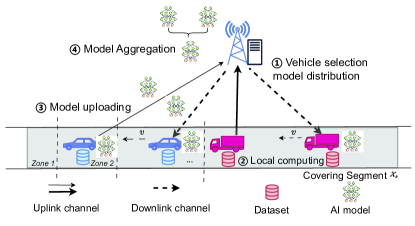
Figure 1: System Model

II Considered Scenario and System Model

II-A Considered Scenario

As shown in Fig. 1, we consider a segment of road covered by a BS with a collaborative server and $K_{0}$ vehicles that arrive at this stretch of road over a period of time. These vehicles will communicate with the BS in the segment of road to train the model through FL paradigm, and each vehicle $k\in\{1,2,\ldots,K_{0}\}$ has collected data samples as $D_{k}$. Here, the data is highly pertinent to vehicular services such as image recognition and trajectory prediction, which has been collected and well-labeled before training. The length of covering segment is $L$, and the segment is divided into multiple zones denoted as $\mathcal{Z}=\{1,2,\ldots,Z\}$. As such, the distance between the vehicle and the BS in the same zone $z\in\mathcal{Z}$ is considered as being the same.

II-B Vehicular Federated Learning Scheme

In the proposed scheme, the training process contains $R$ rounds before the deadline $T_{d}$. The server is able to get the location and velocity of vehicle $k$ within the segment during training as $x_{k}^{t}$ and $v_{k}^{t}$ at $t_{0}<T_{d}$.

During the training process of the MAVFL scheme, the loss function for vehicle $k$ is expressed as

$$f(\mathbf{w}_{k},D_{k})=\frac{1}{|\mathcal{D}_{k}|}\sum_{i\in\mathcal{D}_{k}}\ell(\mathbf{w}_{k};z^{i}_{k}),$$

where $\mathcal{D}_{k}$ means the indices of samples in ${D}_{k}$, $z^{i}_{k}$ is the data sample representation for sample $i\in\{1,2,\ldots,|\mathcal{D}_{k}|\}$ and $\ell$ is the local loss function. Vehicle $k$ will train model $\mathbf{w}$ to find the optimal model as $\hat{\mathbf{w}_{k}}=\arg\min_{\mathbf{w}_{k}}\frac{1}{|\mathcal{D}_{k}|}\sum_{i=1}^{|\mathcal{D}_{k}|}\ell(\mathbf{w}_{k};z^{i}_{k}),$ and the global loss function is $F(w)=\sum_{k=1}^{K}q_{k}f(\mathbf{w}_{k},D_{k}),$ where $q_{k}$ is the aggregation weight of vehicle $k$.

II-B1 Vehicle Selection and Model Distribution

At the beginning of round $r\in\{1,2,\ldots,R\}$, the server owns the newest global model $w^{(r)}$, then it will make the vehicle selection decision to generate the set of vehicles $\mathcal{S}^{r}$ and distribute the model to vehicles within its covering segment as

$$\mathbf{w}^{r,0}_{k}\leftarrow\mathbf{w}^{r},\forall k,x_{k}^{r,0}\in\mathcal{X}_{s},k\in\mathcal{S}^{r},$$ (1)

where $\mathbf{w}^{r,0}_{k}$ means the local model for vehicle $k$ in round $r$ and epoch 0, $\mathcal{X}_{s}$ is the location range of covering segment, and $x_{k}^{r,0}$ is the location of vehicle $k$ at the beginning of round $r$.

II-B2 Local Updating

After receiving model $w^{r,0}_{k}$, vehicle $k$ will perform local stochastic gradient descent (SGD) for $E$ epochs. For local training epoch $e\in\{0,\ldots,E-1\}$, the gradient descent is expressed as $g_{k}^{r,e}\leftarrow\frac{1}{|\mathcal{D}_{k}|}\sum_{i=1}^{|\mathcal{D}_{k}|}\nabla\ell(\mathbf{w}_{k}^{r,e};z^{i}_{k})$ and vehicle $k$ performs local SGD as

$$\mathbf{w}_{k}^{r,e+1}\leftarrow\mathbf{w}_{k}^{r,e}-\eta{g}_{k}^{r,e},\text{for }e\in[0,E-1].$$ (2)

II-B3 Model Uploading

After local updating, vehicle $k$ will try to upload model updates $g^{r}_{k}=\sum_{e=0}^{E-1}g_{k}^{r,e}$ to the server. Due to the movement of vehicles, it may drive out of the covering segment of the BS, which causes the model missing. We define the dropout indicator $\mathbbm{1}_{k}^{r}\in\{0,1\}$ as

$$\mathbbm{1}_{k}^{r}=\left\{\begin{aligned} &1,\quad&x_{k}^{r,E}\in\mathcal{X}_{s},\\ &0,\quad&x_{k}^{r,E}\notin\mathcal{X}_{s}\end{aligned}\right.$$

to represent the state of whether vehicle $k$ stays in the covering segment after local updating with $E$ epochs in round $r$.

II-B4 Model Aggregation

The server will wait for a period of time to receive model updates from vehicles within the covering segment. If the server receives any model updates within $T_{\text{max}}$, it will aggregate these models as

$$\mathbf{w}^{r+1}=\mathbf{w}^{r}-\eta\sum_{k}\mathbbm{1}_{k}^{r}(\frac{g_{k}^{r}}{\sum_{k}{\mathbbm{1}_{k}^{r}}}),\forall\sum_{k}{\mathbbm{1}_{k}^{r}}\neq 0$$ (3)

to get new global model $\mathbf{w}^{r+1}$. For each global model $\mathbf{w}^{r+1}$, we define the set of vehicles as $\mathcal{N}^{r}$ which denotes the set of vehicles uploading models included in the global model as

$$\mathcal{N}^{r}=\mathop{\bigcup}_{k,\forall\mathbbm{1}_{k}^{r}=1}\{k\},$$ (4)

then the successful training ratio $p^{r}$ is denoted as

$$p^{r}=\frac{|\mathcal{N}^{r}|}{|\mathcal{S}^{r}|},$$ (5)

where $|\mathcal{N}^{r}|$ is the number of receiving uploading models from vehicles and $|\mathcal{S}^{r}|$ is the number of vehicles receiving downloading models. The value of $p^{r}$ is related to both vehicle selection and vehicle mobility. Especially, when all vehicles are stationary, the ratio $p^{r}$ is 1, and the ratio is 0 considering all selected vehicles driving out of the covering segment during local computing. When $p^{r}$ is 0, the server will distribute the global model as $\mathbf{w}^{r+1}=\mathbf{w}^{r}$.

II-C Training Delay model

We give the analysis of the delay of the MAVFL scheme in this part. Considering the movement of vehicle $k$, the distance of vehicle $k$ and BS as $L_{k}^{r}$ is related to the topology structure of the road and the movement of vehicles. We define the location coordinate of vehicle $k$ as $x_{k}$, then the distance between vehicle $k$ and BS can be expressed as

$$L_{k}^{r}=\begin{aligned} \sqrt{(L_{z})^{2}+H^{2}},x_{k}^{r}\in\mathcal{Z}_{z},\\ \end{aligned}$$

where $H$ is the height of BS, $L_{z}$ is the normalized distance between vehicle and BS in zone $z$, and $\mathcal{Z}_{z}$ is the range of location for zone $z$.

The uplink transmission for selected vehicles is considered as an orthogonal frequency-division multiple access (OFDMA), then the uplink transmission rate of vehicle $k$ is $q_{k}^{r}=B_{k}\log_{2}\left(1+\frac{P_{k}h_{k}(L_{k}^{r})^{-\beta}}{N_{0}}\right)$ where $B_{k}$ is the bandwidth allocated for vehicle $k$, $P_{k}$ is the transmission power, $h_{k}$ is the channel power gain for vehicle $k$ and $\beta$ is pass loss exponent. Then the uplink time for vehicle $k$ is expressed as $T_{k,\text{c}}^{r}=M/q_{k}^{r}$ with uploading model size $M$.

Next we give the expressions of computation time for vehicle $k$ as $T_{k,\text{p}}=\frac{|\mathcal{D}_{k}|g_{k}}{c_{k}f_{k}},$ where $g_{k}$ is the number of GPU cycles required to train one bit of data, $f_{k}$ is the GPU frequency and $c_{k}$ is the normalized parameter.

Considering the setup of server synchronous aggregation, the duration time for the MAVFL scheme is the sum of communication time and computation time as $T=T_{\text{c}}+T_{\text{p}}=\sum_{r\in\mathcal{R}}\max_{k\in\mathcal{K}}[a_{k}^{r}(T_{k,\text{c}}^{r}+T_{k,\text{p}})]$, where $a_{k}^{r}\in\{0,1\}$ is the indicator representing whether the vehicle is unselected or selected in round $r$. For each selected vehicle, the allocated bandwidth is $B_{k}=B/(\sum_{k}a_{k}^{r})$ with total bandwidth $B$.

III Convergence Analysis

In this section, we give the convergence proof of the MAVFL scheme considering the influence of vehicle mobility. Given the convergence, we assume the below assumptions and lemma are satisfied [9, 10].

Assumption 1.

The loss function $F$ are L-smooth as $\|\nabla F(\mathbf{w}_{1})-\nabla F(\mathbf{w}_{2})\|\leq L\|\mathbf{w}_{1}-\mathbf{w}_{2}\|$ for given $\mathbf{w}_{1}$ and $\mathbf{w}_{2}$.

Assumption 2.

The expected squared norm of stochastic gradients for each vehicle $k$ is upper-bounded: $\mathbb{E}\left\|\nabla f(\mathbf{w}^{r,e}_{k})\right\|^{2}\leq~{}G^{2}$.

Assumption 3.

The variance of mini-batch gradients is upper-bounded: $\left\|g(\mathbf{w})-\nabla f(\mathbf{w})\right\|^{2}\leq\sigma^{2}.$

Assumption 4.

The divergence between local and global loss functions is bounded: $\frac{1}{K}\sum_{k=1}^{K}\left\|\nabla f(\mathbf{w})-\nabla F(\mathbf{w})\right\|^{2}\leq\epsilon_{g}^{2}.$

Lemma 1.

The divergence of the local model and virtual global model is bounded: $\mathbb{E}\left[\sum_{k=1}^{K}\left\|\overline{\mathbf{w}}_{t}-\mathbf{w}_{k}^{t}\right\|^{2}\right]\leq 4K\eta_{t}^{2}(E-~{}1)^{2}G^{2}$.

Based on the above Assumptions 1-4 and Lemma 1, we derive the following theorem to prove the convergence of the proposed scheme.

Theorem 1.

Let $\eta_{t_{0}}\leq 2\eta_{t},\forall t-t_{0}\leq E-1$, then the convergence rate of proposed FL scheme satisfies

$$\frac{1}{T}\sum_{t=1}^{T}\mathbb{E}\bigg{[}\|\nabla F(\bar{\mathbf{w}}^{t})\|^{2}\bigg{]}\leq\frac{1}{T}\sum_{t=1}^{T}\frac{2}{\eta p^{t}}(\mathbb{E}[F(\bar{\mathbf{w}}^{0})]-F_{\mathrm{inf}})$$ (6)

$$+{2(\epsilon_{g})^{2}}+\eta(\delta^{2}+G^{2})L+4\eta^{2}(E-1)^{2}G^{2}L^{2}$$

Proof.

See Appendix A. ∎

Remark 1. From the above theorem, we can get the main factor of convergence in the proposed scheme is the real-time ratio $p^{t}$ in (5). Considering the affecting factors of $p^{t}$, the vehicle selection choice $a_{k}^{r}$ has an important impact on the ratio $p^{t}$, which also influences the convergence speed.

IV Problem Formulation

To minimize the training loss and training delay, we design the utility function which combines the proportion of receiving models and normalized training delay as

$$\Phi^{r}(a_{k}^{r})=[\alpha p^{r}(a_{k}^{r})-(1-\alpha)\frac{T(a_{k}^{r})-T_{\text{min}}}{T_{\text{max}}-T_{\text{min}}}],$$

where $\mathbf{a}^{r}=[a_{1}^{r},a_{2}^{r},\ldots,a_{K}^{r}]$ is the vehicle selection strategy for all vehicles, $\alpha$ is the parameter between 0 and 1 to balance the impact of training loss and delay, and $T_{\text{min}},T_{\text{max}}$ are minimum and maximum of round duration time, respectively. Then we formulate the optimization problem to maximize the sum of utility functions as

$$\mathbf{P1}:\operatorname*{max}_{\mathbf{a}^{r}} \sum_{k}\Phi^{(r)}(a_{k}^{r})$$

$$\mathbf{s.t}. B/\sum_{k}a_{k}^{r}\geq B_{\text{min}},\forall r\in\mathcal{R},k\in\mathcal{K}$$ (7a)

$$a_{k}^{r}\in{0,1},\forall r\in\mathcal{R},k\in\mathcal{K}$$ (7b)

$$\sum_{k}a_{k}^{r}=K_{0},\forall r\in\mathcal{R}$$ (7c)

The inequality in (7a) means the lower bound of bandwidth for each vehicle should be guaranteed. The expression in (7b) indicates the feasibility condition of vehicle selection, and the equality in (7c) gives the number of initially selected vehicles.

The problem P1 is difficult to solve directly because the expression of probability $p^{r}(a_{k}^{r})$ needs future location and velocity information of selected vehicles, which are challenging to get before vehicle selection and training. We design the MAB-based vehicle selection algorithm to solve the optimization problem.

V Proposed Algorithm

In this section, we provide the solution to the problem P1. The proposed vehicle selection problem in P1 can be formulated as an MAB problem [11, 12, 13]. The vehicles with the larger estimated accumulated utility function are selected with the upper confidence bound (UCB) policy.

In the proposed MAB vehicle selection algorithm, the exploitation-exploration trade-off is considered with a larger utility function as exploitation and the diversity of participated vehicles as exploration. The details of exploitation and exploration are shown below.

Algorithm 1 MAB-based vehicle selection algorithm.

1:Location of vehicles $\{x_{k}^{r}\}$, number of vehicles selected $M^{r}$.

2:The set of selected vehicles $\mathcal{S}^{r}$.

3:for $r\leq R$ do

4:     if $r=0$ then

5:         Select $K_{0}$ vehicles randomly as $\mathcal{S}^{0}$ in $\mathcal{K}$.

6:     else

7:         BS calculates the UCB score in (10) and updates score list $\mathcal{U}[k]=U_{k}(a^{r}_{k})$ based on $\mathcal{S}^{r-1}$.

8:         BS generates vehicle set

9:$\mathcal{S}^{r}=$$\{K_{0}\text{ vehicles with largest values of }U_{k}\text{ in }\mathcal{U}\}.$

10:     end if

11:     BS distributes global model to vehicles in $\mathcal{S}^{r}$.

12:end for

V-1 Exploitation

We record the times of vehicle $k$ been selected before round $r$ as

$$M^{(r)}(\lambda,a_{k}^{r})=\sum_{\tau=1}^{r}\lambda^{r-\tau}\mathbbm{1}(a_{k}^{r}=1),$$

where $\lambda$ denotes as discount factor between 0 and 1 to measure the importance of recent choices. Then we can get the discounted empirical average as

$$\bar{\Phi}^{r}(\lambda,a_{k}^{r})=\frac{\sum_{\tau=1}^{r}\lambda^{r-\tau}\mathbbm{1}(a_{k}^{r}=1)\Phi^{(r)}(a_{k}^{r})}{M^{r}(\lambda,a_{k}^{r})}$$ (8)

which gives more weight to recent objective functions.

V-2 Exploration

We give the function of the UCB index of the proposed scheme as

$$c_{k}(\lambda,a_{k}^{r})=\sqrt{\frac{2\log n(r,\lambda)}{M^{r}(\lambda,a_{k}^{r})}},$$ (9)

where $n(r,\lambda)$ records the total number of all the vehicles selected before round $r$. This UCB index function facilitates the selection and exploration of alternative vehicles in other zones. At the beginning of the selection, if vehicle $k$ is not chosen for a while, then $n(r,\lambda)$ will increase with the training and $M^{r}(\lambda,a_{k}^{r})$ remains the same. In subsequent training rounds, vehicle $k$ will be chosen frequently with a larger UCB index. When the vehicle $k$ is selected for many rounds, the parameter $M^{r}(\lambda,a_{k}^{r})$ will increase bringing in a decreasing UCB index.

Based on the above formulations, the upper UCB index in MAVFL scheme is denoted as

$$U_{k}(a_{k}^{r})=\bar{\Phi}^{r}(\lambda,a_{k}^{r})+c_{k}(\lambda,a_{k}^{r}).$$ (10)

During the training process for the largest $K_{0}$ values of $U_{k}$, the vehicle selection choices $a_{k}^{r}$ will be set as 1. All the selection choices are learned from past rounds of UCB scores. The details of the vehicle selection process are described in Algorithm. 1.

VI Simulation Results

VI-A Simulation Setup

In the simulation, we consider a flow of vehicles driving through a straight road with a length of 1,000 m. The mobility pattern of the vehicle is the intelligent driver model, and the base station is situated in the middle of the road with a height of 25 m. For vehicle ML tasks, we consider image classification tasks with the CIFAR-10 dataset and GTSRB dataset, respectively. For the CIFAR-10 dataset, we utilize the ResNet-18 model, and for the GTSRB dataset, we utilize the LeNet model. Each vehicle contains 600 samples with independent identically distributed. Other relevant parameters used in this simulation are listed in Table I.

TABLE I: Simulation Parameters.

Parameter	Description	Value
$\eta$	Learning rate	0.01
$B_{a}$	Batch size	32
$Z$	The number of zones	20
$G_{v}$	BS antenna gain	6 dBi
$l_{p}$	Pass loss model	128.1+37.6$\log_{10}d$
$B$	Bandwidth	3 MHz
$P_{n}$	Noise power	-114 dBm
$v$	vehicle velocity	{60, 80} km/h
$f_{k}$	GPU frequency	1.3 Ghz
$\alpha$	Weight parameter	0.6

The baselines are as follows:

• Communication-based selection (CBS): The vehicles are selected with the nearest distance from the BS with better communication conditions in each round.

• Remain-time based selection (RBS): The vehicles are selected with the longest remaining time in the covering segment in each round.

• Random: The vehicles are selected randomly through the covering segment.

TABLE II: Performance comparison on CIFAR-10 and GTSRB datasets.

	CIFAR-10		GTSRB
	Training delay to 75% accuracy		Training delay to 90% accuracy
Method	Training Delay for 60 km/h (sec.)	Training Delay for 80 km/h (sec.)	Training Delay for 60 km/h (sec.)	Training Delay for 80 km/h (sec)
Proposed	2326.27	2357.96	320.24	339.66
CBS	2812.62($\times$ 1.21)	2558.51($\times$ 1.08)	457.67($\times$ 1.42)	492.72($\times$ 1.45)
RBS	2613.61($\times$ 1.12)	3890.03($\times$ 1.65)	398.5 ($\times$ 1.24)	384.03 ($\times$ 1.13)
Random	2974.8($\times$ 1.27)	N/A	666.14 ($\times$ 2.08)	1298.26 ($\times$ 3.82)

VI-B Simulation Results

In Fig. 2, we compare the training accuracy for the above vehicle selection algorithms with different velocities as 60 km/h and 80 km/h with the CIFAR-10 dataset. From Fig. 2a and 2b, we observe that the convergence speed of the proposed vehicles selection algorithm with MAB is faster, and the overall time of the proposed scheme can be substantially reduced compared to two heuristic and one random algorithms. Moreover, the reduction of the overall time is decreased on average with higher velocity because the number of vehicles is less with larger distance between vehicles.

Figure 3 shows the performance of different algorithms on the GTSRB dataset. We can observe that the convergence speed of the proposed vehicle selection algorithm with MAB is faster than the three baseline algorithms. We note that the improved accuracy in the GTSRB dataset is smaller than in the CIFAR dataset. It is also worth noting that the convergence time required for GTSRB is shorter than CIFAR-10. The reason for these two situations is that the GTSRB dataset is easier to train with fewer training samples compared with CIFAR-10.

Table II shows the results of the delay in target accuracy performance of the proposed scheme with two datasets. Especially, for the CIFAR-10 dataset, we compare the delay of all vehicle selection methods reaching 75% accuracy, and the 90% accuracy is considered for the GTSRB dataset. For the CIFAR-10 dataset, compared with CBS and RBS selection algorithms, the MAB algorithm is nearly 23% faster for 60 km/h, and approximately 50% faster for 80 km/h. In particular, the Random algorithm can not reach 80% accuracy within the given deadline. Meanwhile, the proposed scheme is approximately 32% faster than CBS and RBS methods for the GTSRB dataset.

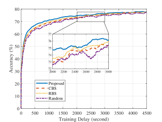
(a) CIFAR-10 with 60 km/h

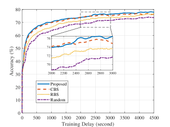
(b) CIFAR-10 with 80 km/h

Figure 2: Training performance of different vehicle selection algorithms for CIFAR-10

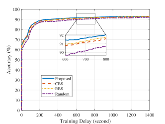
(a) GTSRB with 60 km/h

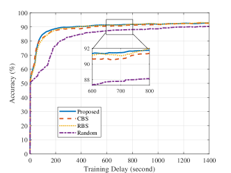
(b) GTSRB with 80 km/h

Figure 3: Training performance of different vehicle selection algorithms for GTSRB

VII Conclusion

In this paper, we have designed an MAVFL scheme and proposed a real-time ratio to reflect the successful training participation rate. We also analyzed the impact of the proposed ratio on convergence results. We have formulated an optimization problem to decrease training delay by selecting suitable vehicles through the MAB-based vehicle selection algorithm. The proposed MAB-based algorithm provides a new feasible solution for real-time vehicle selection. In future work, we will explore the proposed scheme for vehicles with computing and data heterogeneity.

Appendix A Proof of Theorem 1

Based on the definition of the virtual global model as $\bar{\mathbf{w}}^{t+1}=\bar{\mathbf{w}}^{t}-\eta\sum_{k}\mathbbm{1}_{k}^{t}(\frac{g_{k}^{t}}{\sum_{k}{\mathbbm{1}_{k}^{t}}})$, we can get the results in (11). Considering the independence of vehicle mobility and local computing, we can get $\mathbb{E}[\sum_{k}(g_{k}^{t}\mathbb{I}_{k}^{t}/\sum_{k}\mathbb{I}_{k}^{t})]=p^{t}\sum_{k}\nabla f(\mathbf{w}^{t}_{k}),$ which means the expected proportion of the number of model updates obtained by server is $p^{t}$ in round $t$ .

For the second term in (11), we can get the results in (12) at the top of the page. For the third term in (11), we can get the results in (13). Then we substitute the second and third parts in (11) with (12) and (13) and average over all global rounds to finish the proof.

References

- [1] X. Shen, J. Gao, W. Wu, M. Li, C. Zhou, and W. Zhuang, “Holistic network virtualization and pervasive network intelligence for 6G,” IEEE Communications Surveys & Tutorials, vol. 24, pp. 1–30, 2022.
- [2] L. Li, D. Shi, R. Hou, H. Li, M. Pan, and Z. Han, “To talk or to work: Flexible communication compression for energy efficient federated learning over heterogeneous mobile edge devices,” in Proc. IEEE INFOCOM, 2021, pp. 1–10.
- [3] W. Wu, C. Zhou, M. Li, H. Wu, H. Zhou, N. Zhang, X. Shen, and W. Zhuang, “AI-native network slicing for 6G networks,” IEEE Wireless Communications, vol. 29, pp. 96–103, Apr. 2022.
- [4] J. Posner, L. Tseng, M. Aloqaily, and Y. Jararweh, “Federated learning in vehicular networks: Opportunities and solutions,” IEEE Network, vol. 35, no. 2, pp. 152–159, Feb. 2021.
- [5] M. F. Pervej, R. Jin, and H. Dai, “Resource constrained vehicular edge federated learning with highly mobile connected vehicles,” IEEE Journal on Selected Areas in Communications, vol. 41, no. 6, pp. 1825–1844, Jun. 2023.
- [6] B. Li, Y. Jiang, Q. Pei, T. Li, L. Liu, and R. Lu, “FEEL: Federated end-to-end learning with non-IID data for vehicular ad hoc networks,” IEEE Transactions on Intelligent Transportation Systems, vol. 23, no. 9, pp. 16 728–16 740, Sep. 2022.
- [7] T. Zeng, O. Semiari, M. Chen, W. Saad, and M. Bennis, “Federated learning on the road autonomous controller design for connected and autonomous vehicles,” IEEE Transactions on Wireless Communications, vol. 21, no. 12, pp. 10 407–10 423, Dec. 2022.
- [8] B. Xie, Y. Sun, S. Zhou, Z. Niu, Y. Xu, J. Chen, and D. Gunduz, “MOB-FL: Mobility-aware federated learning for intelligent connected vehicles,” in Proc. ICC, 2023, pp. 3951–3957.
- [9] C. Feng, H. H. Yang, D. Hu, Z. Zhao, T. Q. S. Quek, and G. Min, “Mobility-aware cluster federated learning in hierarchical wireless networks,” IEEE Transactions on Wireless Communications, vol. 21, no. 10, pp. 8441–8458, Oct. 2022.
- [10] X. Li, K. Huang, W. Yang, S. Wang, and Z. Zhang, “On the convergence of FedAvg on non-IID data,” 2020. [Online]. Available: https://arxiv.org/abs/1907.02189
- [11] Z. Jiang, Y. Xu, H. Xu, Z. Wang, J. Liu, Q. Chen, and C. Qiao, “Computation and communication efficient federated learning with adaptive model pruning,” IEEE Transactions on Mobile Computing, vol. 23, no. 3, pp. 2003–2021, Mar. 2024.
- [12] M. Li, J. Gao, L. Zhao, and X. Shen, “Adaptive computing scheduling for edge-assisted autonomous driving,” IEEE Transactions on Vehicular Technology, vol. 70, no. 6, pp. 5318–5331, Jun. 2021.
- [13] X. Liu, Y. Deng, and T. Mahmoodi, “Wireless distributed learning: A new hybrid split and federated learning approach,” IEEE Transactions on Wireless Communications, vol. 22, no. 4, pp. 2650–2665, Apr. 2023.