A further study on the renormalization group aspect of perturbative corrections

Abstract

I perform a further study regarding a renormalization-group (RG) issue—which concerns a wide variety of the so-called perturbative power counting under effective field theories (EFT)—as pointed out by A. M. Gasparyan and E. Epelbaum [Phys. Rev. C 107, 034001 (2023)]. I show that the issue could originate from a wrong power counting, or from treating those incomplete, truncated amplitudes beyond the degree to which they should be trusted. Meanwhile, under EFT principles, one should always associate the result with an uncertainty that is adequate to its EFT order. One way to accommodate this is to encode its effect in a more general form of contact terms. In this regard, no RG issue is found in the ³P₀ nucleon-nucleon scattering under the Long and Yang power counting. In contrast, the RG issue under Weinberg’s pragmatic proposal remains a problem even with uncertainty taken into account.

I Introduction

One of the most important developments in modern theoretical physics is the conception of effective field theory (EFT). Pioneered by Weinberg Weinberg (1979); Coleman et al. (1969); Callan et al. (1969); Weinberg (1999), the key concept is to arrange physical observables order-by-order based on an appropriate effective Lagrangian that accommodates the energy scale of interest and the symmetries of the system that one wishes to describe. In contrast to an exact theory—where everything needs to be specified or known—EFT accommodates practical difficulties such as the impossibility of carrying out all of the higher-order calculations, the ignorance of the unknown physics, or both. This leads to the philosophy that physical descriptions should be improved order-by-order based on available information Hartmann (2001). The ignorance of higher-order corrections (regardless of their origin) is compensated by renormalization and is accompanied by the entrance of low-energy constants (LECs). LECs are free parameters in the theory and are normally fitted to observables in order to obtain reasonable descriptions. However, apart from a few cases where physical observables can be obtained analytically such as nuclear forces based on pionless EFT up to the few-body level Hammer et al. (2020) or certain quantum electrodynamics (QED) processes, the fitting processes interfere with the prediction, which can potentially grant inconsistent theories and prevent us from a deeper understanding of nature. Therefore, when numerical solutions are the only possibility, a careful check of the renormalizability of the final results is required. Only after that could one justify whether a consistent approach based on the principles of EFT is obtained.

In nuclear EFT, it is known that currently the most popular arrangement of nuclear forces—Weinberg’s pragmatic proposal (WPP) Weinberg (1990, 1991)—fails to generate renormalizable results Hammer et al. (2020); Grießhammer (2022). This is demonstrated by the breakdown of the renormalization group (RG) invariance of the nucleon-nucleon (NN) scattering amplitude from the leading order (LO) throughout next-to-next-to-next-to-leading order (N³LO) Nogga et al. (2005); Pavón Valderrama and Arriola (2006a, b); Yang et al. (2009a, b); Zeoli et al. (2013), and up to next-to-leading order (NLO) in few-body systems Yang et al. (2021, 2023).

As a consequence, studies Kaplan et al. (1998, 1996); Birse (2007); Long and van Kolck (2008); Pavón Valderrama (2011a, b); Long and Yang (2011, 2012a, 2012b); Wu and Long (2019a); Song et al. (2017); Wu and Long (2019b); Peng et al. (2020); Habashi (2022); Yang et al. (2021, 2023); Thim et al. (2023); Li et al. (2023); Thim et al. (2024); Thim (2024) suggest that a consistent treatment of nuclear forces involves a non-perturbative treatment only at LO. Higher-order corrections are to be added perturbatively under distorted-wave-Born-approximation (DWBA). Note that this treatment has been applied in the context of pionless EFT, where, in addition to numerical analysis, analytic or semi-analytic expressions show strong evidence that RG-invariance is satisfied van Kolck (2020a, b). A recent Bayesian analysis also indicates that its breakdown scale is consistent with $M_{hi}\approx m_{\pi}$ Ekström and Platter (2024).

Despite the above-demonstrated success of the DWBA-based power counting (PC), there are controversies Valderrama (2019); Pavon Valderrama (2019); Epelbaum et al. (2019, 2020). On one hand, numerical analyses show that the RG issues of WPP become severe once the ultraviolet cutoff $\Lambda$ associated with the non-perturbative iteration is increased beyond $1$ GeV. This leads Refs. Epelbaum and Gegelia (2009); Epelbaum et al. (2018a, 2017, b) to argue that one should stay within a limited cutoff window (which normally ranges from $450\sim 600$ MeV), as the non-perturbative treatment at LO already mandated the “peratization” of an EFT for an arbitrarily high cutoff. On the other hand, results generated by PC based on DWBA have certain features that can be either inconvenient or require further studies. The inconvenient feature concerns the possible need to restore missing pole positions (mainly the bound-states) under perturbation theory Contessi et al. (2017); Bansal et al. (2018); Yang et al. (2021); Yang (2024); Contessi et al. (2024a, b). Moreover, a recent study by Gasparyan and Epelbaum Gasparyan and Epelbaum (2023) discovered an interesting feature of perturbative treatment, which leads the authors to claim that a wide variety of DWBA-based PCs are generally not RG invariant. The authors demonstrated their argument by explicit calculations on the NN scattering problem, under a toy model as well as the PC of Long and Yang Long and Yang (2011, 2012a, 2012b). In response, Ref. Peng et al. (2024) advocates that the issue can be avoided by adjusting the fitting strategy to make those exceptional cutoffs amenable to chiral effective field theory.

In this work, the aforementioned RG issue regarding perturbative PCs is further studied under EFT principles. In particular, I will show that the analysis performed in Ref. Gasparyan and Epelbaum (2023) does provide a new and valuable methodology in the aspect of PC-analysis. Nevertheless, it needs to be accompanied by the ingredient that any EFT calculation should be associated with an uncertainty adequate to the given order. Once the uncertainty prescribed by the PC is taken into account, the appeared RG issue disappears in the ³P₀ case for the Long and Yang PC Long and Yang (2011).

The paper is organized as follows. In Sec. II, I argue conceptually that the RG-analysis performed in Ref. Gasparyan and Epelbaum (2023) could suffer from problems of treating the incomplete, truncated amplitudes exactly. A refinement for it to become a meaningful tool in analyzing PCs under EFT is proposed. Then I demonstrated the concept with a toy model in Sect. III. In Sec. IV, the PC of Long and Yang in the NN ³P₀ channel is analyzed using a more general form of contact terms. In Sec. V, the analysis is applied to WPP. Finally, the findings are summarized in Sec. VI.

II RG-analysis with uncertainty taken into account

II.1 General consideration

An EFT-justified calculation must have results organized in an order-by-order improvable manner. Denoting $\mathcal{O}_{n}$ the observable evaluated up to order $n$, it must scale asGrießhammer (2016); Griesshammer (2020); Yang (2020):

$$\mathcal{O}_{n}(M_{lo};\Lambda;M_{hi})=\underbrace{\sum_{i}^{n}\left(\frac{M_{lo}}{M_{hi}}\right)^{i}\mathcal{F}_{i}(M_{lo};M_{hi})}_{\text{trustable part}}$$

$$+\underbrace{\operatorname{\mathscr{C}}_{n}(\Lambda;M_{lo},M_{hi})\left(\frac{M_{lo}}{M_{hi}}\right)^{n+1}}_{\text{uncertainty}},$$ (1)

where $M_{lo}$ denotes the low-energy scales, and $M_{hi}$ is the breakdown scale. The “trustable part” associated with $\mathcal{F}_{i}$ denotes processes that have been evaluated explicitly. The evaluation includes renormalization/fitting to observables. Meanwhile, as long as one stops at a finite $n$, results will always contain a residue $\operatorname{\mathscr{C}}_{n}$, which accounts for the ignorance of higher-order effects. Although the exact form is unknown, for the expansion to work, the uncertainty must contain a suppression $\sim\left(\frac{M_{lo}}{M_{hi}}\right)^{n+1}$, which means that one is more sure about the answer $\mathcal{O}_{n}$ as the order $n$ increases. $\operatorname{\mathscr{C}}_{n}$ must not scale as positive powers of $\Lambda$, otherwise RG is broken. Normally, $\operatorname{\mathscr{C}}_{n}$ oscillates with $\Lambda$ and converges to a constant such that $\left(\frac{\mathscr{C}_{n}}{\mathcal{O}_{n}}\right)\sim O(1)$ after $\Lambda\gg M_{hi}$. Since one usually demands $\mathcal{O}_{n}$ to fall into the vicinity of experimental data $\mathcal{O}_{exp}$, LECs are adjusted in a way so that the difference between the “trustable part” and $\mathcal{O}_{exp}$ is remediable by the “uncertainty”. After the adjustment, effects due to different fitting strategies, $\Lambda$, or the regulator on $\mathcal{O}_{n}$ should be equal or smaller than the “uncertainty” part. This also means a successful EFT only concerns/ensures that $\mathcal{O}_{n}$ is trustable up to an uncertainty that is adequate to the considered order, rather than having an exact value.

II.2 Features at LO with the presence of a singular attractive potential

At LO, a non-perturbative treatment is necessary for at least part of the interactions. This non-perturbative treatment also gives rise to bound-states. Denoting $V_{LO}$ as the LO interaction, the LO amplitude can be obtained by solving the Lippmann-Schwinger equation (LSE), i.e.,

$$T_{LO}(p^{\prime},p;E)=V_{LO}(p^{\prime},p)+\frac{2}{\pi}M\int_{0}^{\infty}\frac{dp^{\prime\prime}\;p^{\prime\prime}{}^{2}\;V_{LO}(p^{\prime},p^{\prime\prime})\;T_{LO}(p^{\prime\prime},p,E)}{p_{0}^{2}+i\varepsilon-p^{\prime\prime}{}^{2}},$$ (2)

where $p_{0}^{2}/M=E_{cm}$ is the cm energy, $M=939$ MeV is the nucleon mass.

Adopting the short-hand operator form as described in Ref. Long and Yang (2011), the NLO correction is

$$T_{NLO} =V_{NLO}+V_{NLO}GT_{LO}+T_{LO}GV_{NLO}$$

$$+T_{LO}G\,V_{NLO}\,GT_{LO}\,,$$ (3)

with

$$G=\frac{2}{\pi}M\int_{0}^{\infty}\frac{p^{\prime\prime}{}^{2}dp^{\prime\prime}}{p_{0}^{2}+i\varepsilon-p^{\prime\prime}{}^{2}}.$$ (4)

One can denote the LO intereaction as

$$V_{LO}=[V^{(L)}_{LO}+V^{(S)}_{LO}]f_{R}(\Lambda),$$ (5)

where $f_{R}(\Lambda)$ is a regulator of choice, and $V^{(L)}_{LO}$ and $V^{(S)}_{LO}$ are the long- and short-range components, respectively. Note that the operator form in the above equations is adopted, with the $(p^{\prime},p)$ applies implicitly.

For convenience, one can further define

$$V^{(S)}_{LO}=\sum_{i=1}^{d_{lo}}C_{i}v_{i},$$ (6)

where $C_{i}$ is the LEC, $d_{lo}$ is the upper limit of the derivative at LO, and $v_{i}$ is the corresponding operator structure. For example, with $V^{(L)}_{LO}$ being the one-pion-exchange potential (OPE), $V^{(S)}_{LO}=C_{T}$ in ³S₁-³D₁ and $V^{(S)}_{LO}=C_{P}pp^{\prime}$ in ³P₀ channel.

Note that the NN potential can be singular and attractive in certain partial-waves, and it is known that the LEC within $V^{(S)}_{LO}$—which is adjusted to renormalize $V^{(L)}_{LO}$—then has a limit-cycle behavior Long and van Kolck (2008) and diverges at specific values of $\Lambda$. This is illustrated below in Fig. 1 and Fig. 2.

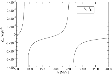
Figure 1: The renormalization constant $C_{T}$ for the LO ³S₁-³D₁ channel as a function of cutoff $\Lambda$, where a sharp cutoff $f_{R}(\Lambda)=\theta(\Lambda)$ is adopted. This plot is taken from Fig. 2 of Ref. Yang et al. (2008).

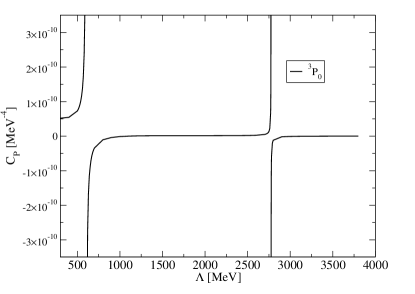
Figure 2: The renormalization constant $C_{P}$ for the LO ³P₀ channel as a function of cutoff $\Lambda$, where a sharp cutoff $f_{R}(\Lambda)=\theta(\Lambda)$ is adopted.

Note that the non-perturbative treatment is equivalent to an eigen-value problem with Hamiltonian $H=KE+V_{LO}$, where $KE$ denotes the kinetic term. After diagonalization, one obtains the LO wavefunction $|\psi_{LO}\rangle_{i}$ and eigenvalues $E_{i}=p_{i}^{2}/M$. $E_{i}$ is continuous for scattering states. At cutoffs ($\equiv\Lambda^{*}$) where the LEC ($\equiv C_{x}$) diverges, $|\psi_{LO}\rangle_{i}$ has a special property, i.e.,

$$\langle\psi_{LO}|v_{x}f_{R}(\Lambda^{*})|\psi_{LO}\rangle_{i}=0,\text{ for all }p_{i}.$$ (7)

Eq. (7) then allows $C_{x}\langle\psi_{LO}|v_{x}f_{R}(\Lambda^{*})|\psi_{LO}\rangle_{i}$ to be finite at the limit $C_{x}\rightarrow\infty$. The peculiar feature of Eq. (7) is guaranteed for all $\Lambda$ listed in Fig. 1 and Fig. 2, as all eigenvalues must be finite after diagonalization.

It needs to be stressed that, the key, i.e., the non-perturbative treatment, must be employed for the above to hold.

However, if a new interaction $V_{new}$ is adopted—which can contain a set of operators with a structure different from $V^{(S)}_{LO}$ (e.g., higher derivative terms), or with the same structure of $V^{(S)}_{LO}$ but with different regulators or cutoff (e.g., $\Lambda_{NLO}\neq\Lambda_{LO}$)—then its matrix element is no longer protected by the eigenvalue properties. This is the very origin of the RG issue for DWBA-based PCs as investigated in Ref.Gasparyan and Epelbaum (2023), and will be analyzed further in the following sections.

II.3 Dilemma at next-to-leading order for DWBA

Consider now the next-to-leading order (NLO) correction from DBWA. The calculation follows perturbation theory and involves the matrix elements consisting of NLO operators sandwiched by $|\psi_{LO}\rangle_{i}$. Define the NLO interactions as

$$V_{NLO}=[V^{(L)}_{NLO}+V^{(S)}_{NLO}]f_{R}(\Lambda),$$ (8)

where

$$V^{(S)}_{NLO}=\sum_{i=1}^{d_{nlo}}C^{(nlo)}_{i}v_{i},$$ (9)

with $C_{i}^{(nlo)}$ the NLO LECs, and $d_{nlo}\geq d_{lo}$ the upper limit of the derivative at NLO. The NLO correction to $E_{i}$ is then

$$E_{i}^{NLO}=\langle\psi_{LO}|V_{NLO}|\psi_{LO}\rangle_{i}.$$ (10)

In general, the short-range part of the NLO interaction, $V^{S}_{NLO}$, has a richer structure than its LO correspondence. Thus, the special property as listed in Eq. (7) will no longer hold. Consequently, the matrix element of a new NLO operator can be zero only at $p_{0}=p_{x}$, but finite elsewhere. This leads to a dilemma if one chooses to renormalize the LEC to an observable at $p_{x}$. On one hand, for this term to have a non-zero correction at $p_{x}$, the corresponding LEC would need to be $\infty$. However, since Eq. (7) does not apply anymore, a diverged LEC will cause the results to diverge for all other $p_{0}\neq p_{x}$. More generally, when a set of operators enters (which is standard for NLO and higher orders), their linear combination, when coupled with the ingredient that at least a subset of the LECs are fixed by a particular renormalization procedure, leads to the same dilemma. The above is referred to as “not factorizable zero” in Ref. Gasparyan and Epelbaum (2023).

As long as $V_{LO}$ is singular and attractive, the LO wavefunction will oscillate more and more at a shorter distance (or equivalently, higher momentum) so that in general one can always find a $p_{x}$ where the “not factorizable zero” occurs at NLO. In practice, the cutoff window where $p_{x}$ falls into the physical region (below $M_{hi}$) can be rather narrow. Nevertheless, it exists. It is demonstrated in Fig. 5 of Ref. Gasparyan and Epelbaum (2023) that the “exceptional cutoff” ($\equiv\Lambda_{e}$) occurs between 2.6990 and 2.6991 GeV for the PC of Long and Yang at NLO.

II.4 Origin of the dilemma and its solution

Ref. Gasparyan and Epelbaum (2023) considered the above dilemma as an RG problem, arguing that the origin of it is due to that the non-perturbative LO amplitude is not “properly renormalized”. In their following works Gasparyan and Epelbaum (2022); Gasparyan et al. (2024), the authors further explicated that the non-perturbative treatment at LO imposes “nontrivial constraints on a choice of the effective interaction and the renormalization scheme”, and one would need to perform subtractions in all possible subdiagrams in the spirit of the Bogoliubov-Parasiuk-Hepp-Zimmermann (BPHZ) renormalization procedure to ensure renormalizability of subleading results.

However, one should keep in mind that any fitting/renormalization procedure of LECs should always take uncertainty into account. In other words, an observable calculated under EFT should always be accompanied by an uncertainty prescribed by the PC. For example, within DWBA, the NLO correction is evaluated by sandwiching the NLO operators with the LO wavefunction $|\psi_{LO}\rangle$—which itself comes with a theoretical uncertainty of size $\lesssim|\psi_{NLO}\rangle$. Thus, although it is not commonly required (neither practiced in Ref. Long and Yang (2011, 2012a, 2012b)), formally, one should always include this uncertainty in the renormalization/fitting procedure, instead of directly solving a set of linear equations to obtain the LECs exactly following a fixed fitting procedure.

Back to the aforementioned issue of Long and Yang PC, the fact that one needs to fix the fitting procedure and fine-tune the cutoff to a precision more than five significant digits for the resulting LECs to give the problematic phase shift (as shown in Fig. 5 and Fig. 6 in Ref. Gasparyan and Epelbaum (2023)) is an indication that the RG issue might come from an illegal demand that requires DWBA to be more accurate than what it should be at the order considered. Note that such a fine-tune-related issue is different from the scenario of a PC failure. When a PC fails, the “uncertainty” part in Eq. (1) is either not under control at all (e.g., diverges / oscillates with $\Lambda$, such as WPP at LO in the singular and attractive channels) or scales worse than the prescribed PC (which could be the case of the NN ¹S₀ channel under WPP or the PC of Ref. Long and Yang (2012b)). On the other hand, a fine-tune-related problem has the “uncertainty” part under control, and the problem only occurs when one demands an accuracy exceeding the uncertainty governed by EFT.

One way to verify whether the RG problem is due to a PC failure or the illegal demand of precision is to take the uncertainty into account when performing the RG analysis. This can be achieved by encoding the uncertainty into a more general form of regulator. The simplest case will be a combination of two regulators, i.e.,

$$\mathfrak{F}_{R}(\Lambda)\equiv xf_{a}(\Lambda)+(1-x)f_{b}(\Lambda),$$ (11)

where $f_{a}$ and $f_{b}$ are regulators with a slight difference. They should be chosen appropriately so that varying the parameter $x$ between 0 and 1 will induce an uncertainty on $\mathcal{O}_{n}$ (observables calculated up to order $n$) smaller or equal to the value prescribed by the PC. Note that $x$ is not an LEC, but a means to incorporate uncertainty. Effectively, $x$ is merely a free and extra parameter one can utilize to avoid the aforementioned fine-tune-related problems. Since $\mathfrak{F}_{R}(\Lambda)$ in Eq. (11) is linear in $x$, to check whether $f_{a}$ and $f_{b}$ are chosen properly for a given order $n$, it is sufficient to evaluate whether the difference between the two extreme cases is smaller than the prescribed uncertainty, that is,

$$|\langle\psi_{LO}|(V^{L}_{NLO}+V^{S}_{NLO})\left(f_{a}(\Lambda)-f_{b}(\Lambda)\right)|\psi_{LO}\rangle_{i}|\lesssim\mathcal{O}_{n}(M_{lo};\Lambda;M_{hi})\left(\frac{M_{lo}}{M_{hi}}\right)^{n+1},\text{ for all }p_{i}\leq M_{hi}.$$ (12)

Note that one caveat in the above equation is that $V^{S}_{NLO}$ contains LECs, and a diverged LEC could cause the matrix element to blow up, rendering Eq. (12) useless. As the purpose of varying $x$ from 0 to 1 is to generate an uncertainty permitted at a given order in the matrix element, any check using Eq. (12) should be evaluated at a typical cutoff where the size of $V^{L}_{NLO}$ is comparable to $V^{S}_{NLO}$.

III Toy model in NN ³P₀ scattering

I now incorporate Eq. (12) to examine the toy model specified in Ref. Gasparyan and Epelbaum (2023). The LO potential is

$$V^{(^{3}P_{0})}_{LO}=[V^{(^{3}P_{0})}_{1\pi}+C_{P}pp^{\prime}]f_{R}(\Lambda_{0}),$$ (13)

where $V^{(^{3}P_{0})}_{1\pi}$ is the OPE in the ³P₀ channel. At NLO,

$$V^{(^{3}P_{0})}_{NLO}=[\bar{V}^{(^{3}P_{0})}_{2\pi}+C^{NLO}_{0}pp^{\prime}]f_{R}(\Lambda_{2}),$$ (14)

where the labeling $\Lambda_{0}$ and $\Lambda_{2}$ is just to denote that the cutoffs are not necessarily the same in each order. $\bar{V}^{(^{3}P_{0})}_{2\pi}$ is the “simplified” version of the two-pion-exchange potential (TPE) in the ³P₀ channel defined in Ref. Gasparyan and Epelbaum (2023), i.e., it comes from the partial-wave decomposition of a less divergent TPE,

$$\bar{V}_{2\pi}(\vec{p}^{\prime},\vec{p})=V_{2\pi}(\vec{p}^{\prime},\vec{p})\frac{(3m_{\pi})^{2}}{(3m_{\pi})^{2}+q^{2}},$$ (15)

where $m_{\pi}$ is the pion mass, $V_{2\pi}$ is the long-range part of TPE, and $q^{2}=(\vec{p}^{\prime}-\vec{p})^{2}$. $\bar{V}_{2\pi}$ has the same singularity as OPE and is accompanied by only one counter term with LEC $C^{NLO}_{0}$ at NLO. Note that $f_{R}$ in Eqs. (13) and (14) denote any type of function that regulates the high-momentum part of the interaction. The following choice,

$$f_{R}(\Lambda)\equiv 0^{n}F(\Lambda)+(1-0^{n})F(\Lambda/2),$$ (16)

where $n=0(1)$ for LO(NLO), coincides to the toy model illustrated in Fig. 2 of Ref. Gasparyan and Epelbaum (2023). $F(\Lambda)$ denotes a sharp cutoff, i.e.,

$$F(\Lambda;p^{\prime},p)=\theta(\Lambda-p^{\prime})\theta(\Lambda-p).$$ (17)

Eq. (16) imposes a cutoff at NLO which is half of the LO value. One could nevertheless absorb this effect into the definition of $V_{NLO}$. The task now is to examine whether the PC based on DWBA is appropriate in this scenario. A straightforward check, as performed in Fig. 2 of Ref. Gasparyan and Epelbaum (2023), shows a problematic RG behavior. However, as stated above, one needs to incorporate the corresponding uncertainty into account. In this toy model, the only way to cure the RG problem is to revert the cutoff from $\Lambda/2\rightarrow\approx\Lambda$ at NLO. When translated into Eq. (12), it means the following needs to be satisfied for the perturbative PC to make sense:

$$|\langle\psi_{LO}|(V^{(^{3}P_{0})}_{2\pi}+C_{0}^{NLO}p^{\prime}p)\left(F(\Lambda/2)-F(\Lambda)\right)|\psi_{LO}\rangle_{i}|\lesssim\mathcal{O}_{n}(M_{lo};\Lambda;M_{hi})\left(\frac{M_{lo}}{M_{hi}}\right)^{n+1},\text{ for all }p_{i}\leq M_{hi},$$ (18)

Here the value of $n+1$ depends on the power counting scheme, but in general $\gtrsim 1$, since it is at least one order suppressed than LO.

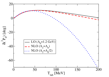
Figure 3: Phase shifts at LO and NLO as a function of laboratory energy $T_{lab}$ for the toy model of Ref. Gasparyan and Epelbaum (2023). The renormalization is performed at $T_{lab}=40$ MeV for all cases. Sharp cutoffs $\Lambda=\Lambda_{0}$ or $\Lambda_{0}/2$ are adopted.

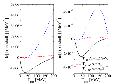
Figure 4: The corresponding real and imaginary part of the on-shell T-matrix for the toy model where the phase shifts are presented in Fig. 3.

The phase shifts up to NLO are plotted as a function of $T_{lab}$ in Fig. 3. As one can see, the adoption of $\Lambda_{2}=\Lambda_{0}/2$ at NLO leads to a more than $200\%$ difference for phase shifts at $T_{lab}>100$ MeV. As shown in Fig. 4, the corresponding NLO T-matrix under $\Lambda_{2}=\Lambda_{0}/2$ becomes larger than the LO value, in contrast to the case where $\Lambda_{2}=\Lambda_{0}$ is adopted. Thus, the problematic pattern as shown in Fig. 2 of Ref. Gasparyan and Epelbaum (2023) will persist unless one prescribes that the NLO uncertainty is more than twice of the value at LO. Therefore, one has to conclude that the DWBA-based PC indeed does not work for the toy model potentials listed in Eqs. (13)-(14).

IV The PC proposed by Long and Yang in the ³P₀ channel

In this section the same analysis is applied to the PC of Long and Yang in the ³P₀ channel Long and Yang (2011), where the LO potential is the same as Eq. (13). At $O(Q^{2})$, instead of Eq. (14), one has

$$V^{(^{3}P_{0})}_{NLO}=[V^{(^{3}P_{0})}_{2\pi}+C^{NLO}_{0}pp^{\prime}+D_{0}^{NLO}pp^{\prime}(p^{2}+p^{\prime 2})]f_{R}(\Lambda_{0}).$$ (19)

Note that the label “NLO” here is adopted for convenience and is interchangeable with $O(Q^{2})$ defined in Ref. Long and Yang (2011). It is the first non-vanishing correction to LO in this channel, but not the first overall correction if one considers all partial-waves. Therefore, it is labeled as “NNLO” in the PC of Long and Yang.

As explained in Sect. II, the fact that the aforementioned RG issue Gasparyan and Epelbaum (2023) occurs only at an extremely narrow window of cutoffs can be an indication that it is merely an artifact of demanding unreasonable precision in the $O(Q^{2})$ renormalization procedure. From Fig. 5 of Ref. Gasparyan and Epelbaum (2023), it might be already clear that a direct combination of two sharp cutoffs, i.e., with $f_{b}=f_{a}(\Lambda-0.001$ GeV) in Eq. 11 would solve the issue of exceptional cutoffs. In the following, I demonstrate that instead of a direct shift in the cutoff, a small uncertainty can be encoded using the following generalized regulator:

$$\mathfrak{F}_{R}=xf_{a}+(1-x)f_{b},$$ (20)

where

$$\begin{split}f_{a}(\Lambda,p^{\prime},p)&=\theta(\Lambda-p^{\prime})\theta(\Lambda-p),\\ f_{b}(\Lambda,p^{\prime},p)&=SG(\Lambda,p^{\prime})SG(\Lambda,p),\\ \end{split}$$ (21)

with

$$\begin{split}SG(\Lambda,p^{(\prime)})&=1\text{ \ \ \ \ \ \ \ \ \ \ \ \ \ \ \ \ \ \ if $p^{(\prime)}\leq\Lambda/1.1$,}\\ &=\exp(\frac{p^{(\prime)20}}{(\Lambda/1.1)^{20}})\text{ if $p^{(\prime)}>\Lambda/1.1$}.\end{split}$$ (22)

Thus, the original sharp cutoff is replaced by a combination of sharp cutoff and Super-Gaussian regulator when one takes the choice $x=0$. Here the order of the Super-Gaussian regulator is taken to be very high so that $f_{b}$ is only slightly different from $f_{a}$.

In Fig. 5, the T-matrix and phase shifts at a typical cutoff $\Lambda=2.640$ GeV are plotted in the left column, while the same quantities near the problematic cutoff (where “exceptional zero” occurs) are shown in the middle ($\Lambda=2.69808$ GeV) and the right ($\Lambda=2.69918$ GeV) column. Note that the exceptional cutoff $\Lambda\approx 2699$ MeV is very close to the cutoff where the LO LEC diverges (as shown in Fig. 2). Nevertheless, the LO amplitude is well-defined and can be obtained numerically by the subtractive renormalization scheme Yang et al. (2009a). Here I adopted the same renormalization procedure as performed in Ref. Gasparyan and Epelbaum (2023), i.e., the LECs are fixed at $T_{lab}=50$ MeV at LO and $T_{lab}=25,50$ MeV at $O(Q^{2})$.

In Fig. 5, the issue of “exceptional zero” is reflected in the red dashed-line in the middle and right columns, where the phase shifts diverge from their “typical cutoff values” (the red dashed-line in (d)). This is because extreme LECs are required to generate finite corrections as the matrix elements go to zero. On the other hand, the problem disappears when the value $x=0$ is taken in Eq. (20), which is demonstrated by the fact that the blue dotted line remains unchanged throughout all panels in Fig. 5. Furthermore, panel (a) shows that, under a typical cutoff, the maximum uncertainty generated by Eq. (20)—which corresponds to a direct change from adopting a regulator that is fully $f_{a}$ to $f_{b}$—produces a difference that is negligible compared to the LO amplitude and is certainly smaller than the uncertainty prescribed by the PC at $O(Q^{2})$. In other words, the variation of $x\in[0,1]$ indeed corresponds to taking into account an uncertainty allowed by EFT.

Note that as long as $x$ has a fixed value throughout all $\Lambda$, “exceptional cutoffs” will only be shifted but still occur. Thus, $x$ should be varied whenever necessary to avoid the problem. In fact, once Eq. (12) is satisfied, not fixing $x$ to an exact value corresponding to not taking the LO wavefunction too exact—as it should be under any EFT. By coupling this uncertainty into the renormalization procedure, one is able to retain a converged pattern in both T-matrix and phase shifts, therefore avoiding the appearance of extreme LECs. The phase shift as a function of $\Lambda$ is plotted in Fig. 6, where $x$ is varied between $0\sim 1$ whenever necessary to avoid taking an accuracy that exceeds the prescribed PC. As one can see, the issue of “exceptional zero” in the Long and Yang PC represented by the two vertical red-dashed lines disappears when one avoids taking an unreasonable accuracy beyond $O(Q^{2})$ in the renormalization process.

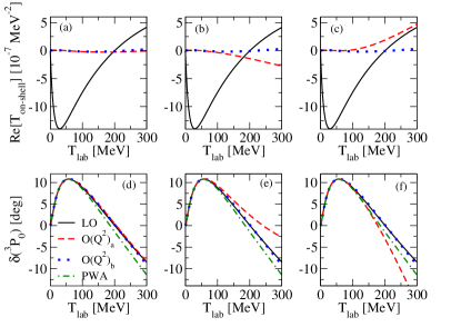
Figure 5: Lower (upper) panels: Phase shifts (real part of the on-shell T-matrix) up to $O(Q^{2})$ as a function of laboratory energy $T_{lab}$ for the Long and Yang PC Long and Yang (2011). The renormalization is performed at $T_{lab}=50$ MeV at LO and $T_{lab}=25$, 50 MeV at $O(Q^{2})$ for all cases. The left panel ((a) & (d)) shows the result for a typical cutoff ($\Lambda=2640$ MeV), whereas the middle ((b) & (e)) and right ((c) & (f)) panels correspond to the cutoff values slightly below ($\Lambda=2698.08$ MeV) and above ($\Lambda=2699.18$ MeV) the exceptional point. $O(Q^{2})_{a}$ and $O(Q^{2})_{b}$ denote the regulators $f_{a}$ and $f_{b}$ in Eq. (21). The LO regulator is $f_{a}$.

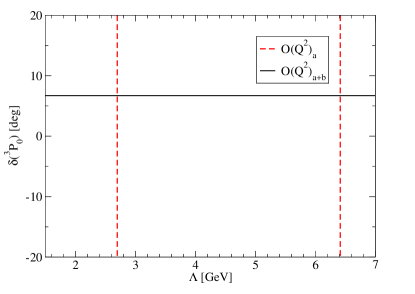
Figure 6: Cutoff dependence of ³P₀ phase shift at $T_{lab}=130$ MeV calculated using Long and Yang PC at $O(Q^{2})$. The red-dashed lines denote the diverged results at the exceptional cutoffs using the regulator $f_{a}$ in Eq. (21). The black solid line denote the results from the generalized regulator with an adjustable $0\leq x\leq 1$ whenever necessary to avoid fine-tune related problems, as defined in Eq. (20).

V Application on the conventional WPP

One might wonder whether the above ingredient, i.e., by taking uncertainty into account when performing renormalization, can resolve the RG issues of WPP. At LO, WPP has been shown to miss appropriate counter terms in those singular and attractive channels Nogga et al. (2005). The problem is of mathematical origin, i.e., singular potentials render the solution of Schrödinger equation undetermined without the presence of a proper boundary condition. Note that the problematic cutoff (where the phase shift deviates from the typical value) first appears at $\approx 1000$ MeV and spans at least for 200 MeV, as demonstrated in the ³P₀ channel panel of Fig. 9 in Ref. Nogga et al. (2005).

Starting at NLO under WPP, the problem persists in two types of pathology. The first has the same origin, i.e., the boundary condition, as LO. For example, the TPE($Q^{2}$) in ³P₀ channel is repulsive at the origin and dominates OPE at short distances. Thus, imposing a counter term “$C^{NLO}pp^{\prime}$” to renormalize OPE+TPE($Q^{2}$) causes an RG problem. The second type of RG problem concerns a Wigner-bound-like effect, which occurs when two counter terms are included non-perturbatively. As the increase of $\Lambda$, the short-range counter terms dominate over pion-exchange and one approaches the regime governed by Wigner-bound Wigner (1955); Phillips and Cohen (1997), which is reflected in, e.g., the NLO S-waves under WPP Yang et al. (2009b). Note that the problematic cutoff starts at $\Lambda\approx 1000$ MeV and spans at least for 100 MeV for both NLO($Q^{2}$) and NNLO($Q^{3}$).

The broadness of the problematic cutoff ($\sim 100-200$ MeV for $\Lambda\approx 1000$ MeV) under WPP is in sharp contrast to those found in the Long and Yang PC ($\sim 0.1$ MeV for $\Lambda\approx 1000$ MeV) without considering the uncertainty. As demonstrated in the previous sections, the uncertainty allowed by EFT at a given order may be encoded into a small change in the regulator or cutoff. It is of interest to see whether those problematic cutoffs under WPP can be eliminated by the uncertainty argument. A naive estimate can be performed as follows. Denoting $\Lambda$ and $\Delta$ the starting value and the broadness of the problematic cutoff, and $Q^{d}$ the leading divergence of the potential in momentum space. Then in the spirit of Eq. (12), the minimum requirement for legally including a small uncertainty in terms of the cutoff/regulator to eliminate the problematic region is

$$\frac{(\Lambda+\Delta)^{d}-\Lambda^{d}}{\Lambda^{d}}\leq(\frac{M_{lo}}{M_{hi}})^{n+1},$$ (23)

where $n$ is the order specified by the PC. Note that the above only counts the difference of the regulator’s impact on the potential at the shortest range. The actual requirement involves an integral over $\int_{\Lambda}^{\Lambda+\Delta}dp$ for the potential together with the wavefunctions on the left-hand side, which in general results in a much stricter requirement. Thus, the left-hand side might need to be much smaller than the right-hand side. Applying the above to WPP at NLO($Q^{2}$), one has

$$\frac{(\Lambda+\Delta)^{2}-\Lambda^{2}}{\Lambda^{2}}=2\frac{\Delta}{\Lambda}+\frac{\Delta^{2}}{\Lambda^{2}}\approx 2\frac{\Delta}{\Lambda},$$ (24)

where the last step assumes $\Delta<<\Lambda$. Plugging $\Lambda\approx 1000$ MeV and $\Delta\approx 100$ MeV, the left-hand side of Eq. (23) $\approx 0.2$. Meanwhile, the right-hand side of Eq. (23) gives $(1/3)^{2}=1/9\approx 0.11$. Applying the same $\Lambda$ and $\Delta$ to NNLO($Q^{3}$) results in a worse violation of Eq. (23). Since the minimum requirement is not even met, this suggests that the problem of WPP cannot be resolved by taking uncertainty into account.

VI Summary

A peculiar type of RG issue under DWBA as discovered in Ref. Gasparyan and Epelbaum (2023) is further studied by taking the theoretical uncertainty into account. It is shown that the problem concerning “exceptional zero” can have two sources: (i) from enforcing an accuracy exceeding the prescribed PC in the wavefunctions/observables at the given order, or, (ii) from a wrong arrangement of PC. In general, the broadness of the problematic cutoff serves as a guide to distinguish the two cases. With a detailed investigation, it is shown that the RG issue for PC of Long and Yang belongs to the former, while the toy model in Ref. Gasparyan and Epelbaum (2023) belongs to the latter. By applying the same argument to WPP, it is found that the RG/Wigner-bound problem is not likely to be resolved by taking uncertainty into account.