Superluminal signalling witness for quantum state reduction with correlated noise

Abstract

Models for quantum state reduction address the quantum measurement problem by suggesting weak modifications to Schrödinger’s equation that have no observable effect at microscopic scales, but dominate the dynamics of macroscopic objects. Enforcing linearity of the master equation for such models ensures that modifications to Schrödinger’s equation do not introduce a possibility for superluminal signalling. In large classes of quantum state reduction models, however, and in particular in all models employing correlated noise, formulating a master equation for the quantum state is prohibitively difficult or impossible. Here, we formulate a witness for superluminal signalling that is applicable to generic quantum state reduction models, including those involving correlated noise. We apply the witness to several relevant cases, and find that correlated-noise models in general allow for superluminal signalling. We suggest how specific models may be able to avoid it, and that the witness introduced here provides a stringent guide to constructing such models.

Introduction — Quantum mechanics has been shown to be non-local by the violation of Bell inequalities in (loophole-free) Bell test experiments Bell (1987); Freedman and Clauser (1972); Aspect et al. (1981, 1982); Hensen et al. (2015); Giustina et al. (2015); Shalm et al. (2015). Despite the non-local evolution of quantum states evidenced by the violations of Bell inequalities, the Bell tests are well-known not to allow faster-than-light communication or superluminal signalling (SLS) Wiseman (2014); Bennett et al. (1993); Boschi et al. (1998); Bouwmeester et al. (1997). The projective and probabilistic nature of quantum measurement renders the local observers in Bell test setups incapable of distinguishing the effect of measurements or quantum operations performed at causally disconnected events.

Quantum measurement itself, meanwhile, remains one of the central open problems of modern physics, being at odds with the unitary time evolution prescribed by Schrödinger’s equation Komar (1962); Wigner (1963); Adler (2003); Bassi et al. (2013). Models for dynamical quantum state reduction (DQSR) attempt to resolve this dichotomy by proposing alterations of Schrödinger’s equation that are weak enough to allow the time evolution of microscopic objects to be indistinguishable from unitary quantum dynamics, while their collective effect on macroscopic objects such as measurement devices causes an arbitrarily fast reduction of the quantum state to a classical state Bassi et al. (2013); Van Wezel (2010); van Wezel (2008). In order for DQSR to be able to result in distinct and stable macroscopic measurement outcomes, starting from the measurement of identical microscopic quantum states, models of DQSR are necessarily stochastic and non-unitary. To obtain the correct Born rule statistics of measurement outcomes, they moreover need to be non-linear Mertens et al. (2021).

The non-unitary and non-linear nature of DQSR models imply that in general they will allow for superluminal signalling. This is avoided in specific DQSR models by insisting that their ensemble averaged state evolution is described by linear quantum semi-group dynamics, in the form of a Gorini-Kosakowsky-Sudarshan-Lindblad (GKSL) type master equation Bassi and Hejazi (2015); Gisin (1989). This is a sufficient condition for preventing SLS, but its practical use is hampered by the fact that explicit expressions for the ensemble averaged state evolution are often prohibitively hard to formulate. In particular, DQSR models employing correlated (colored) noise as their stochastic component rarely allow for closed-form master equations Mukherjee and van Wezel (2024a). Here, we therefore introduce an alternative, sufficient and necessary condition for avoiding SLS, in the form of a ‘witness’ observable whose non-zero instantaneous expectation value indicates SLS. The witness can be straightforwardly evaluated in any DQSR model, including those based on correlated as well as white noise. We show that it agrees with the linear semi-group condition whenever the latter can be assessed, and demonstrate its use beyond those cases by analysing several recently-proposed DQSR models employing correlated noise. We find that they all allow SLS in general, and discuss the limits in which SLS may be avoided. The witness introduced here thus provides stringent constraints on the construction of DQSR models, guiding in particular the further exploration of models based on correlated noise.

SLS witness — All models for DQSR have a limit in which they produce instantaneous projective measurement, with outcomes distributed according to Born’s rule. This is usually the thermodynamic limit of infinitely large or heavy measurement machines. DQSR models smoothly connect the instantaneous projective dynamics of this limit to the continuous unitary evolution of Schrödinger’s equation that is observed in the opposite, microscopic limit of small or light objects. This implies the existence of a mesoscopic regime, in which evolution is neither unitary, nor instantaneous. It is the existence of this mesoscopic regime that potentially allows for SLS.

To create superluminal signals, one requires a sender (say Alice) who is space-like separated from a recipient (Bob), with whom she shares a known entangled state. Entanglement is a necessary resource, because relativistic classical physics does not allow SLS, while product states contain only local information for each observer. Alice and Bob can potentially send signals using DQSR dynamics if at least one of them operates in the mesoscopic regime where DQSR deviates from both unitary evolution and instantaneous projections. We therefore consider the situation in which Alice performs a measurement on her half of the entangled state using a mesoscopic measurement device. This causes non-unitary DQSR dynamics lasting a finite, non-zero amount of time before resulting in a stable measurement outcome and final state. During or after this time, Bob can perform an instantaneous, projective measurement of his half of the entangled state using a truly macroscopic measurement apparatus. We will separately consider the situation in which both Alice and Bob employ a mesoscopic device in the discussion section, and show that it does not yield opportunities for SLS beyond those already present if only Alice uses a mesoscopic device.

Without loss of generality, we consider a two-state superposition and write the initial configuration as $\ket{M_{A}}(\alpha(0)\ket{0}_{A}\ket{0}_{B}+\beta(0)\ket{1}_{A}\ket{1}_{B})\ket{M_{B}}$. Here $\ket{M_{A,B}}$ are states for the measurement devices of Alice and Bob, while the states labeled by $A$ ($B$) subscripts describe Alice’s (Bob’s) part of the shared entangled quantum state. As Alice performs a measurement with her mesoscopic device, but before Bob does anything, the system evolves to von Neumann (2018); Bassi and Ghirardi (2003); Bassi et al. (2013):

$$\left[\,\alpha(\xi_{t},t)\ket{M_{A}^{0}(t)}\ket{0(\xi_{t},t)}_{A}\ket{0}_{B}\right.\phantom{]}$$

$$\left.+\,\beta(\xi_{t},t)\ket{M_{A}^{1}(t)}\ket{1(\xi_{t},t)}_{A}\ket{1}_{B}\,\right] \ket{M_{B}}$$ (1)

Here $|M_{A}^{0,1}(t)\rangle$ indicate the state of the measurement device evolving differently in the two components of the wave function. Moreover, the non-linear DQSR dynamics may cause both the values of the coefficients $\alpha$ and $\beta$, and Alice’s quantum state to evolve in time. How these evolve will depend not only on time, but also on the (time-dependent) values of stochastic parameter(s) $\xi_{t}$ appearing in the particular DQSR model under consideration. That is, DQSR models are defined in terms of a stochastic differential, in which the evolution of the quantum state at time $t$ depends on the instantaneous value(s) of a (set of) stochastic parameters(s) $\xi_{t}$. Notice however, that the stochastic parameters $\xi_{t}$ themselves evolve in time independently from the quantum state. In each realisation of the DQSR dynamics, the outcome is determined by the particular instance of $\xi_{t}$ encountered, and expectation values are defined as the average over an ensemble of realisations of the stochastic parameter(s).

For simplicity, we ignore the Schrödinger evolution of Bob’s quantum state (i.e. we work in a co-rotating frame). Crucially, because only Alice’s measurement device is affected by the non-unitary and non-linear aspects of the DQSR evolution, and because we assume Alice’s device to be localised within her neighbourhood, the DQSR dynamics does not cause evolution of Bob’s quantum state or measurement device.

At some point during the evolution described by Eq. (1), Bob performs a projective measurement and instantaneously reduces the state of the full system to either $\ket{M_{A}^{0}(t)}\ket{0(\xi_{t},t)}_{A}\ket{0}_{B}\ket{M_{B}^{0}}$, with probability $|\alpha(\xi_{t},t)|^{2}$, or to $\ket{M_{A}^{1}(t)}\ket{1(\xi_{t},t)}_{A}\ket{1}_{B}\ket{M_{B}^{1}}$, with probability $|\beta(\xi_{t},t)|^{2}$. Because Bob’s projective dynamics is probabilistic, he will not be able to glean any information from the one measurement outcome obtained in just a single measurement. We will thus allow for Alice and Bob to share an infinitely large ensemble of known, identically prepared entangled states. Moreover, we assume that both Alice and Bob can perform simultaneous but independent measurements on all their states, so that they can measure ensemble averages and determine outcome probabilities within the time required for a single measurement.

If Bob can decide based on his own measurement outcomes whether or not Alice started performing measurements on her side, this constitutes signalling across space-like separated events. Formally, SLS is therefore avoided if and only if:

$$\mathbb{E}_{\xi}\left[\left.\langle\hat{I}^{A}\otimes\hat{O}^{B}\rangle\right|\mathcal{M}^{A}_{\xi}\right]=\mathbb{E}_{\xi}\left[\left.\langle\hat{I}^{A}\otimes\hat{O}^{B}\rangle\right|\mathcal{I}^{A}\right]~{}~{}\forall\hat{O}^{B}$$ (2)

Here, $\mathbb{E}_{\xi}[\langle\hat{O}\rangle|\mathcal{M}]$ indicates the ensemble average of measurement outcomes when Bob measures observable $\hat{O}$, conditional on Alice evolving her state according to the map $\mathcal{M}$. Notice that this involves both an average over all possible paths $\xi_{t}$ that the stochastic parameters in Alice’s DQSR evolution can take, and the usual quantum expectation value averaging over possible outcomes of Bob’s projective measurement. The operator $\hat{I}^{A}\otimes\hat{O}^{B}$ has support only on Bob’s half of the entangled state, while $\mathcal{M}^{A}_{\xi}$ indicates evolution according to a DQSR model with stochastic parameter $\xi_{t}$ caused by Alice’s mesoscopic measurement device, and the identity map $\mathcal{I}^{A}$ indicates Alice does not perform any measurement or operation.

If the two expectation values in Eq. (2) are equal for all possible local observables $\hat{I}^{A}\otimes\hat{O}^{B}$ and all possible initial configurations, it is impossible for Bob to distinguish between Alice performing a measurement using DQSR dynamics and Alice not doing anything at all. In contrast, the violation of Eq. (2) for even a single observable or initial state implies the possibility of superluminal signalling between Alice and Bob.

Writing the initial entangled quantum state as the Schmidt decomposition $\sum_{j}\alpha_{j}\ket{j}_{A}\ket{j}_{B}$, Eq. (2), takes on the form of a particularly convenient witness:

$$\mathbb{E}_{\xi}\left[\left|\alpha_{j}(\xi_{t},t)\right|^{2}\right]=\left|\alpha_{j}(0)\right|^{2}~{}~{}\forall j$$ (3)

Whenever the ensemble averaged value of coefficients in the Schmidt basis changes as a consequence of Alice’s DQSR evolution, Bob can measure this using projective measurements. At any point in time, deviations of the instantaneous ensemble average from its initial value thus serve as a witness for superluminal signalling. Conversely, if Eq. (3) is satisfied for all time, the DQSR dynamics cannot be used for superluminal signalling.

Signalling — To see explicitly how the witness can be used to exclude superluminal communications, first consider the extreme limit in which both Alice and Bob employ instantaneous projective measurements. In that case the initial state $\ket{M_{A}}(\alpha(0)\ket{0}_{A}\ket{0}_{B}+\beta(0)\ket{1}_{A}\ket{1}_{B})\ket{M_{B}}$ will be instantaneously reduced by Alice to either $\ket{M_{A}^{0}}\ket{0}_{A}\ket{0}_{B}\ket{M_{B}}$, with probability $|\alpha(0)|^{2}$, or to $\ket{M_{A}^{1}}\ket{1}_{A}\ket{1}_{B}\ket{M_{B}}$, with probability $|\beta(0)|^{2}$. The consecutive measurement by Bob will with certainty produce either the state $\ket{M_{B}^{0}}$ or $\ket{M_{B}^{1}}$ for Bob’s measurement machine. The overall probability for Bob to register the result $\ket{M_{B}^{0}}$ is thus $|\alpha(0)|^{2}$, which is the same as it would have been had Bob acted directly on the initial state without Alice doing anything. Notice that adding the possibility for Alice to act with local unitary operators on her state does not affect this result, as these do not change the values of the coefficients in the wave function, nor the state at Bob’s side. Under arbitrary Schrödinger evolution and instantaneous collapse, the witness thus remains zero and Bob cannot distinguish between Alice performing a measurement or not.

Next, consider the situation in which Alice causes evolution according to some DQSR model, but with her evolution reaching a final state before Bob does his measurement. If the DQSR model correctly describes evolution ending on stable measurement outcomes, the state just before Bob initiates his measurement will be either $\ket{M_{A}^{0}}\ket{0(\xi_{t},t)}_{A}\ket{0}_{B}\ket{M_{B}}$, with some probability $P_{0}(\xi)$, or $\ket{M_{A}^{1}}\ket{1(\xi_{t},t)}_{A}\ket{1}_{B}\ket{M_{B}}$, with probability $P_{1}=1-P_{0}$. As before, Bob’s measurement outcome can be predicted by Alice with certainty in either case, and Bob registers $\mathbb{E}_{\xi}[P_{0}(\xi)]$ as the overall probability for obtaining the outcome $\ket{M_{B}^{0}}$. Because Alice and Bob are allowed to know the initial state (for example because they prepared it together in the past), Bob will know that Alice acted with DQSR dynamics whenever $\mathbb{E}_{\xi}[P_{0}(\xi)]\neq|\alpha(0)|^{2}$ and the witness is nonzero. To avoid SLS, any model for DQSR must thus ensure that within an ensemble of stochastic evolutions, the stable end states representing measurement outcomes are obtained with Born rule probabilities. Moreover, this must hold for all possible initial states.

Finally, consider the case of Alice causing DQSR dynamics, and Bob imposing a projective measurement before Alice’s device reaches a stable measurement outcome. The state just before Bob measures is then given by Eq. (1), and Bob obtains the outcome $\ket{M_{B}^{1}}$ with probability $\mathbb{E}_{\xi}[\,|\alpha(\xi_{t},t)|^{2}]$. Again, Bob can compare this probability with the known value $|\alpha(0)|^{2}$ that he would obtain if Alice does nothing. In order to avoid SLS, the ensemble averaged squared values of components in the Schmidt basis must therefore always remain equal to their initial values: $\mathbb{E}_{\xi}[|\alpha_{j}(\xi_{t},t)|^{2}]=|\alpha_{j}(0)|^{2}$ for all components $j$ and all times $t$. This condition renders probability dynamics under SLS-avoiding DQSR evolution a so-called Martingale process Bassi and Ghirardi (2003), and shows that deviations of DQSR dynamics from being Martingale serve as a witness for SLS.

Necessary and sufficient — So far, we proved the condition of Eq. (3) to be necessary for guaranteeing the absence of superluminal signalling, by formulating an explicit protocol causing SLS when it is violated. That the condition is also sufficient follows from the fact that as long as Eq. (3) is satisfied, expectation values of operators acting locally on Bob’s states are constant in time. Bob can therefore not use any instantaneous projective measurement to distinguish the state of Eq. (1) from the situation in which Alice does not cause DQSR dynamics.

This leaves only the most general case of Bob and Alice both using DQSR dynamics to be considered. Because DQSR dynamics is non-linear, the combination of two simultaneous mesoscopic measurements requires further specification. We interpret it as the $dt\to 0$ limit of a series of time intervals of length $dt$, in which Alice and Bob alternate in causing DQSR dynamics while the other does nothing. This definition keeps the form of the DQSR dynamics caused by Alice independent from whether or not Bob chooses to do a measurement, while allowing the two measurements to affect each other through their dependence on the evolving values of the wave function coefficients. If Eq. (3) is satisfied during both of the individual DQSR processes, the ensemble average $\mathbb{E}_{\xi}[\,|\alpha(\xi_{t},t)|^{2}]$ remains constant during each time step, and the expectation values of all local observables remain constant for all time. Even in this most general circumstance, adherence to the condition of Eq. (3) is thus necessary and sufficient to preclude superluminal signalling.

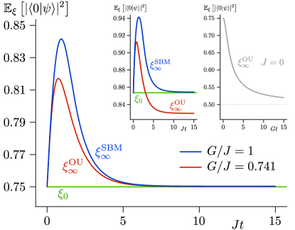
Figure 1: The witness $\mathbb{E}_{\xi}\left[\left|\alpha_{j=0}(\xi_{t},t)\right|^{2}\right]$ of Eq. (3) as a function of time for various DQSR models, evaluated using the dynamics specified in Eq. (5). The evolutions in the main panel all start from $\alpha(0)=\cos(\pi/6)$. A constant value of the witness indicates that the possibility of SLS is precluded. The green lines labeled $\xi_{0}$ show the limit of zero correlation time encountered in CSL as well as SUV models in the white-noise limit. The red and blue lines labeled $\xi_{\infty}$ indicate the opposite limit of infinitely correlated (constant) noise in the two-state SUV model, with noise values sampled either from the steady state of an Ornstein-Uhlenbeck (OU) process, or from spherical Brownian Motion (SBM). The former causes SLS for long times because there is no value of the ratio $G/J$ that allows the witness the return to its initial value for all possible initial conditions, as shown in the left inset ($\alpha(0)=\cos(\pi/8)$, but the same values of $G/J$ as the main panel). This is shown to be possible for SBM noise, but a non-constant value of the witness, and hence SLS, cannot be avoided at short times and constant noise values. The grey line in the right inset shows that a model with linear state evolution ($J=0$) will violate the no-signalling condition at all times. All expectation values shown are numerically averaged over $10^{6}$ implementations of the noise.

Correlated noise — Having identified a witness for SLS, we can apply it to specific models for DQSR. All DQSR models introduce weak perturbations to Schrödinger’s equation and can be written in the form of coupled Itô stochastic differential equations:

$$d\ket{\psi_{t}} =\left(-i\,\hat{H}_{t}\,dt+d\hat{\mathcal{G}}_{t}\right)\ket{\psi_{t}}$$

$$d\hat{\mathcal{G}}_{t}\ket{\psi_{t}} =\hat{J}_{t}(\psi_{t},\xi^{\mu}_{t})\ket{\psi_{t}}dt+\sum_{\nu}\hat{G}^{\nu}_{t}(\psi_{t},\xi^{\mu}_{t})\ket{\psi_{t}}dW^{\nu}_{t}$$

$$d\xi^{\mu}_{t} =f(\xi^{\mu}_{t})dt+g(\xi^{\mu}_{t})dW^{\mu}_{t}$$ (4)

Here $\hat{H}_{t}$ is the standard (possibly time dependent) Hamiltonian and $d\hat{\mathcal{G}}_{t}$ is the modification to time evolution defining the DQSR model. Its terms $\hat{J}_{t}$ and $\hat{G}^{\nu}_{t}$ may be (non-linear) functions of the state $\ket{\psi_{t}}$ and may further depend on a set of independent (possibly temporally correlated or colored) Markovian stochastic processes $\xi^{\mu}_{t}$ with continuous trajectories, indexed by $\mu\in\mathbb{Z}^{+}$. They follow independent Itô stochastic differential equations (i.e. the noise average $\mathbb{E}_{\xi}[\xi_{t}^{\mu}\xi_{s}^{\nu}]=0~{}\forall\mu\neq\nu$), in which $f$ and $g$ are smooth functions on their respective sample spaces Mukherjee et al. (2024); Mukherjee and van Wezel (2024a). Here $dW^{\mu,\nu}_{t}$ are all independent identically distributed Gaussian increments denoting a standard Wiener process (corresponding to the Brownian motion $W_{t}=\int\,dW_{t}$) Revuz and Yor (1999); Øksendal (2003); Gardiner (2004).

The first class of DQSR models in this general formulation for which we consider the SLS witness is the well-known family of Continuous Spontaneous Localization (CSL) models Pearle (1989); Bassi and Ghirardi (2003); Ghirardi et al. (1990). Applied to an initial two-state superposition, they are defined by:

$$d\hat{\mathcal{G}}_{t}\ket{\psi_{t}} =\left[\frac{-\gamma}{2}\left(\hat{\sigma}-\langle\hat{\sigma}\rangle_{t}\right)^{2}dt+\sqrt{\gamma}\left(\hat{\sigma}-\langle\hat{\sigma}\rangle_{t}\right)dW_{t}\right]\ket{\psi_{t}}$$

Here $\gamma$ is a constant and $\hat{\sigma}$ is a Pauli-$\sigma_{z}$ operator. We consider the setup described before where the initial state contains products of the states of local measurement machines of Alice and Bob as well as a shared entangled state. The Pauli operator is then defined in terms of the states $|M_{A}^{0,1}(t)\rangle$ describing Alice’s measurement device. Notice that this model has only uncorrelated (white) noise described by $dW_{t}$. The recently introduced family of models for DQSR known as Spontaneous Unitarity Violation (SUV) Van Wezel (2010); van Wezel (2008); Mertens et al. (2021); Mukherjee et al. (2024); Mukherjee and van Wezel (2024a, b), also have a white-noise limit that falls in this class of CSL models Mukherjee and van Wezel (2024a, b).

For these white-noise models, a GKSL-type master equation can be formulated, obeying the Martingale property for its probability dynamics Bassi and Ghirardi (2003); Mukherjee and van Wezel (2024a). The witness of Eq. (3) is then analytically verified to be zero for all time, precluding the possibility of SLS. This is indicated by the green line in Fig. 1, where $\xi_{0}$ indicates the vanishing correlation time of noise in CSL models.

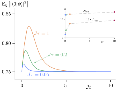
Figure 2: The witness $\mathbb{E}_{\xi}\left[\left|\alpha_{j=0}(\xi_{t},t)\right|^{2}\right]$ of Eq. (3) as a function of time for the SUV model with correlated SBM noise. The lowest (blue) curve is for correlation time $J\tau=0.05$, the middle (green) one for $J\tau=0.2$, and the top (orange) line for $J\tau=1$. For each evolution, the value of $J/G$ was adjusted to ensure the emergence of Born’s rule at long times. The inset shows that the time $Jt_{\text{max}}$ at which the maximum deviation of the witness from its initial value occurs, shifts to later times for larger correlation times. Despite this, it always stay well below the collapse time $Jt_{\text{coll}}$, defined as the characteristic decay time of the off-diagonal expectation value $\mathbb{E}_{\xi}\left[\alpha_{j=0}(\xi_{t},t)\alpha_{j=1}(\xi_{t},t)\right]$. All expectation values shown are numerically averaged over $10^{5}$ implementations of the noise.

Several models with correlated noise have been considered in the case of SUV Mertens et al. (2021, 2023, 2024); Mukherjee et al. (2024). For a two-state superposition, their dynamics is given by:

$$d\hat{\mathcal{G}}_{t}\ket{\psi_{t}} =\left(J\langle\hat{\sigma}\rangle_{t}+G\xi_{t}\right)\left(\hat{\sigma}-\langle\hat{\sigma}\rangle_{t}\right)dt\ket{\psi_{t}}$$ (5)

The overall geometric factor introduced by the final expectation value in this expression ensures norm-preserving dynamics, while the non-linear term proportional to $J$ induces stable end points for the evolution at $\langle\hat{\sigma}\rangle=0,1$, corresponding to the two possible measurement outcomes. The stochastic parameter $\xi_{t}$ is assumed to be temporally correlated, and obeys the independent stochastic dynamics $d\xi_{t}=-\xi_{t}dt/\tau+g(\xi_{t})dW_{t}$. Here, $\tau$ is the correlation time for the noise. Although any generic continuous stochastic process may be utilized for $\xi_{t}$, two processes of particular interest are the (Gaussian) Ornstein-Uhlenbeck process (OU) with $g(\xi_{t})=\sqrt{{2}/{\tau}}$ and the spherical Brownian motion (SBM) defined by $g(\xi_{t})=\sqrt{{1-\xi_{t}^{2}}/{\tau}}$ Mertens et al. (2021, 2023, 2024); Mukherjee and van Wezel (2024a).

In the limit of infinite correlation time (static noise), the results of numerically evaluating Eq. (5) is depicted by the red and blue lines in Fig. 1. For SBM noise, it is possible to find a ratio $G/J$ such that Born’s rule is obeyed at long times for all possible initial conditions. This precludes SLS in the long time limit. At short times, however, there is a clear deviation from the witness $\mathbb{E}_{\xi}[|\alpha_{j=0}(\xi_{t},t)|^{2}]$ being constant, and the possibility of SLS is unavoidable. Moreover, for OU noise, SLS is unavoidable even at long times, because there is no value of $G/J$ that allows the witness to return to its initial value for all initial states simultaneously Mertens et al. (2024).

For intermediate values of the correlation time in SUV models with SBM noise, Fig. 2 shows that the short-time deviation of $\mathbb{E}_{\xi}\left[\left|\alpha_{j=0}(\xi_{t},t)\right|^{2}\right]$ from its initial value disappears smoothly in the limit of vanishing correlation time, but cannot be avoided for any finite value. The time at which the maximum deviation occurs shifts to higher values for longer correlation times of the noise, but stays well below the characteristic time over which the evolution approaches its stable end points (as shown in the inset of Fig. 2). As the parameter $J$ in SUV models scales extensively with system size, more macroscopic measurement machines cause faster DQSR dynamics. The possibility of SLS, indicated by the witness deviating from a constant value, therefore occurs within a vanishingly short time-interval in the thermodynamic limit.

Discussion — We showed that white-noise DQSR models may avoid the possibility of SLS, while known DQSR models based on correlated noise unavoidably encounter SLS when applied to two-state superpositions. Nevertheless, we stress that this does not imply one should only consider white-noise models going forward. Firstly, white noise, with strictly zero correlation time, does not occur anywhere in nature. If it is to arise from a physical process, the best one can achieve is an effectively stochastic process with arbitrarily small correlation time. That this should be considered fundamentally distinct from white noise when considering DQSR dynamics follows from the scaling of the collapse time with inverse system size. For any given value of the correlation time, regardless how small, there will be a critical size for measurement machines, above which the DQSR evolution takes place entirely within the correlation time of the noise. SLS is then unavoidable for macroscopic measurement machines obeying the types of DQSR dynamics considered above. The effect of the SLS witness not being constant may be unobservable in practice if it occurs only within an unmeasurably short interval, but that it cannot be avoided in principle should raise questions about the existence of closed time-like loops.

Secondly, while we did not identify any DQSR processes with correlated noise capable of avoiding SLS, we did not show such processes cannot exist. Moreover, we only considered the DQSR evolution of two-state superpositions, keeping open the possibility that more general initial states may allow for SLS-free dynamics.

Conclusions — In conclusion, we showed that Eq. (3) provides both a necessary and sufficient condition for any model introducing changes to Schrödinger’s equation to preclude the possibility of superluminal signalling. This applies in particular to models for dynamical quantum state reduction. We showed that the condition is satisfied in white noise models for dynamical state reduction in which the absence of superluminal signalling is known to be guaranteed by linearity of the effective master equation. The condition of Eq. (3), however, can be straightforwardly checked also for models in which the master equation cannot be obtained. We gave explicit examples of this for specific models with correlated noise, which we showed to allow superluminal signalling at short times, even if they conform to Born’s rule at long times.

Besides the models considered here, some correlated-noise extensions of known white-noise DQSR models have been proposed Adler and Bassi (2007, 2008). To the best of our knowledge it is currently not known whether they will be able to satisfy Eq. (3) at all times, and we are therefore unaware of any correlated-noise DQSR model that can guarantee the absence of superluminal signalling altogether. This does not imply such a model does not exist, however. In fact, we argue that if dynamical state reduction, or any other type of modified Schrödinger dynamics, is caused by a physical process, it cannot be fundamentally white and will have to obey Eq. (3) in order to avoid superluminal signalling. The condition formulated here thus provides a stringent requirement as well as a clear guiding principle in the ongoing search for a fully satisfactory model of dynamical quantum state reduction.

References

- Bell (1987) J. S. Bell, Speakable and unspeakable in quantum mechanics (Cambridge University Press, 1987).
- Freedman and Clauser (1972) S. J. Freedman and J. F. Clauser, Phys. Rev. Lett. 28, 938 (1972).
- Aspect et al. (1981) A. Aspect, P. Grangier, and G. Roger, Phys. Rev. Lett. 47, 460 (1981).
- Aspect et al. (1982) A. Aspect, J. Dalibard, and G. Roger, Phys. Rev. Lett. 49, 1804 (1982).
- Hensen et al. (2015) B. Hensen, H. Bernien, A. E. Dréau, A. Reiserer, N. Kalb, M. S. Blok, J. Ruitenberg, R. F. L. Vermeulen, R. N. Schouten, C. Abellán, W. Amaya, V. Pruneri, M. W. Mitchell, M. Markham, D. J. Twitchen, D. Elkouss, S. Wehner, T. H. Taminiau, and R. Hanson, Nature 526, 682 (2015).
- Giustina et al. (2015) M. Giustina, M. A. M. Versteegh, S. Wengerowsky, J. Handsteiner, A. Hochrainer, K. Phelan, F. Steinlechner, J. Kofler, J.-A. Larsson, C. Abellán, W. Amaya, V. Pruneri, M. W. Mitchell, J. Beyer, T. Gerrits, A. E. Lita, L. K. Shalm, S. W. Nam, T. Scheidl, R. Ursin, B. Wittmann, and A. Zeilinger, Phys. Rev. Lett. 115, 250401 (2015).
- Shalm et al. (2015) L. K. Shalm, E. Meyer-Scott, B. G. Christensen, P. Bierhorst, M. A. Wayne, M. J. Stevens, T. Gerrits, S. Glancy, D. R. Hamel, M. S. Allman, K. J. Coakley, S. D. Dyer, C. Hodge, A. E. Lita, V. B. Verma, C. Lambrocco, E. Tortorici, A. L. Migdall, Y. Zhang, D. R. Kumor, W. H. Farr, F. Marsili, M. D. Shaw, J. A. Stern, C. Abellán, W. Amaya, V. Pruneri, T. Jennewein, M. W. Mitchell, P. G. Kwiat, J. C. Bienfang, R. P. Mirin, E. Knill, and S. W. Nam, Phys. Rev. Lett. 115, 250402 (2015).
- Wiseman (2014) H. Wiseman, Nature 510, 467– (2014).
- Bennett et al. (1993) C. H. Bennett, G. Brassard, C. Crépeau, R. Jozsa, A. Peres, and W. K. Wootters, Phys. Rev. Lett. 70, 1895 (1993).
- Boschi et al. (1998) D. Boschi, S. Branca, F. De Martini, L. Hardy, and S. Popescu, Phys. Rev. Lett. 80, 1121 (1998).
- Bouwmeester et al. (1997) D. Bouwmeester, J. W. Pan, K. Mattle, M. Eibl, H. Weinfurter, and A. Zeilinger, Nature 390, 575– (1997).
- Komar (1962) A. Komar, Phys. Rev. 126, 365 (1962).
- Wigner (1963) E. P. Wigner, Am. J. Phys. 31, 6– (1963).
- Adler (2003) S. L. Adler, Stud. Hist. Phil. Science B 34, 135 (2003).
- Bassi et al. (2013) A. Bassi, K. Lochan, S. Satin, T. P. Singh, and H. Ulbricht, Rev. of mod. phys 85, 471–527 (2013).
- Van Wezel (2010) J. Van Wezel, Symmetry 2, 582 (2010).
- van Wezel (2008) J. van Wezel, Phys. Rev. B 78, 054301 (2008).
- Mertens et al. (2021) L. Mertens, M. Wesseling, N. Vercauteren, A. Corrales-Salazar, and J. van Wezel, Phys. Rev. A 104, 052224 (2021).
- Bassi and Hejazi (2015) A. Bassi and K. Hejazi, Eur. J. Phys. 36, 055027 (2015).
- Gisin (1989) N. Gisin, Helv. Phys. Acta 62, 363 (1989).
- Mukherjee and van Wezel (2024a) A. Mukherjee and J. van Wezel, Phys. Rev. A 109, 032214 (2024a).
- von Neumann (2018) J. von Neumann, in Mathematical Foundations of Quantum Mechanics, edited by N. A. Wheeler (Princeton University Press, 2018).
- Bassi and Ghirardi (2003) A. Bassi and G. Ghirardi, Phys. Rep. 379, 257 (2003).
- Mukherjee et al. (2024) A. Mukherjee, S. Gotur, J. Aalberts, R. van den Ende, L. Mertens, and J. van Wezel, Entropy 26, 131 (2024).
- Revuz and Yor (1999) D. Revuz and M. Yor, Continuous martingales and Brownian motion (Springer Berlin, 1999).
- Øksendal (2003) B. Øksendal, Stochastic differential equations: An introduction with applications (Springer Berlin, 2003).
- Gardiner (2004) C. W. Gardiner, Handbook of stochastic methods for physics, chemistry and the natural sciences (Springer Berlin, 2004).
- Pearle (1989) P. Pearle, Phys. Rev. A 39, 2277 (1989).
- Ghirardi et al. (1990) G. C. Ghirardi, P. Pearle, and A. Rimini, Phys. Rev. A 42, 78 (1990).
- Mukherjee and van Wezel (2024b) A. Mukherjee and J. van Wezel, (2024b), arXiv:quant-ph/2405.01077 .
- Mertens et al. (2023) L. Mertens, M. Wesseling, and J. van Wezel, SciPost Phys. 14, 114 (2023).
- Mertens et al. (2024) L. Mertens, M. Wesseling, and J. van Wezel, SciPost Phys. Core 7, 012 (2024).
- Adler and Bassi (2007) S. L. Adler and A. Bassi, J. Phys. A: Math. Theor. 40, 15083 (2007).
- Adler and Bassi (2008) S. L. Adler and A. Bassi, J. Phys. A: Math. Theor. 41, 395308 (2008).