Solvers for mixed finite element problems using Poincaré operators based on spanning trees

Wietse M. Boon NORCE Norwegian Research Centre, Nygårdsgaten 112, 5008 Bergen wibo@norceresearch.no
Abstract.

We propose an explicit construction of Poincaré operators for the lowest order finite element spaces, by employing spanning trees in the grid. In turn, a stable decomposition of the discrete spaces is derived that leads to an efficient numerical solver for the Hodge-Laplace problem. The solver consists of solving four smaller, symmetric positive definite systems. We moreover place the decomposition in the framework of auxiliary space preconditioning and propose robust preconditioners for elliptic mixed finite element problems. The efficiency of the approach is validated by numerical experiments.

2020 Mathematics Subject Classification:
65N22, 65N30, 65F08

1. Introduction

Mixed finite element methods are capable of preserving the structure of partial differential equations and thereby mimic physical behavior of a system at the discrete level. Stability and convergence of these methods can be derived rigorously using underlying theory [6, 9]. However, the incorporation of physical conservation laws often leads to large saddle point problems that are computationally demanding to solve. Thus, efficient numerical solvers are essential to keep simulation times manageable. In this work, we propose such solvers by leveraging spanning trees in the grid.

The use of spanning trees in mixed finite element discretizations and solvers dates back, at least, to the tree-cotree decomposition of the Raviart-Thomas space of [5]. Later, they were employed in [17, 1] to construct representatives of the first cohomology group of the de Rham complex. In [3], a spanning tree was employed to construct divergence-free finite element spaces. The key idea there is to restrict an $H(\operatorname{curl})$-conforming finite element space by setting the edge degrees of freedom on a spanning tree to zero. This creates a subspace that is linearly independent of the kernel of the $\operatorname{curl}$ and, in turn, its image under the $\operatorname{curl}$ forms a basis for a divergence-free subspace of $H(\operatorname{div})$. This strategy was then generalized to higher-order spaces in [2, 16, 4]. We note that in [2], the authors moreover employed a spanning tree of the dual graph to compute finite element functions with assigned divergence. This same strategy was later employed in [11, 10] to ensure mass conservation in reduced order models.

In this paper, we build on these results by casting spanning tree decompositions in the framework of Finite Element Exterior Calculus [7, 6]. In this light, these decompositions allow us to explicitly construct Poincaré operators for the finite element de Rham complex. In turn, we use these Poincaré operators to decompose the finite element space into a subspace related to a spanning tree, and a subspace that lies in the kernel of the differential. This provides a novel perspective on the constructions from [3, 2, 16] and extends the ideas to more general, exact sequences.

We highlight two practical implications that arise from the derived theory. First, the decomposition provides a different basis for the finite element spaces. Expressed in this basis, the Hodge-Laplace problem becomes a series of four smaller, symmetric positive definite systems that can be solved sequentially, without loss of accuracy. We show numerically that this results in a significant speed-up for all Hodge-Laplace problems on the complex, especially for the problem posed on the facet-based Raviart-Thomas space.

Second, we fit the derived decomposition in the framework of auxiliary space preconditioning to construct a preconditioner for elliptic problems. We show that the performance of this preconditioner is related to the Poincaré constant on a subspace of the decomposition. This Poincaré constant is computable and forms an upper bound on the Poincaré constant of the full finite element space. Numerical experiments indicate that the preconditioner is particularly well-suited for problems in which the terms involving the differential dominate, which implies that it properly handles the large kernel of the differential operator.

We note that our construction is reminiscent of the regular decomposition from [18] with a notable difference that our decomposition does not contain a high-frequency term. Moreover, this work draws inspiration from [14], in which Poincaré operators are constructed for the twisted and BGG complexes.

The remainder of this paper is organized as follows. First, Section 1.1 introduces preliminary concepts such as exact sequences and the discrete de Rham complex. Our main theoretical results are presented in Section 2, where we construct a Poincaré operator that leads to a decomposition of the finite element spaces. Using this decomposition, we propose a solver for the Hodge-Laplace problem in Section 3. In Section 4, we then construct a preconditioner for elliptic finite element problems by placing the decomposition in the framework of auxiliary space preconditioning. We present numerical experiments in Section 5 that highlight the potential of these approaches. Section 6 contains concluding remarks.

1.1. Preliminary definitions and notation conventions

An exact sequence is a series of vector spaces $\Lambda^{k}$ and a differential mapping $d_{k}:\Lambda^{k}\to\Lambda^{k+1}$, indexed by $k\in\mathbb{Z}$, with the property $\operatorname{Ran}(d_{k},\Lambda^{k})=\operatorname{Ker}(d_{k+1},\Lambda^{k+1})$. In other words, the range of $d_{k}$ coincides with the kernel of the next operator $d_{k+1}$. The subscript $k$ is omitted when clear from context. An exact sequence can be illustrated as

(1.1) ${\cdots}$ ${\Lambda^{k-1}}$ ${\Lambda^{k}}$ ${\Lambda^{k+1}}$ ${\cdots}$ $\scriptstyle{d}$ $\scriptstyle{d}$ $\scriptstyle{d}$ $\scriptstyle{d}$

and we denote this sequence by $(\Lambda^{\bullet},d)$. By the defining property of an exact sequence, two consecutive steps in this diagram maps to zero, i.e. $dd=0$. We continue by introducing a concept that is fundamental to this work, namely Poincaré operators.

Definition 1.1.

A Poincaré operator for an exact sequence $(\Lambda^{\bullet},d)$ is a family of linear maps $p_{k}:\Lambda^{k}\to\Lambda^{k-1}$ that satisfies

(1.2) $\displaystyle d_{k-1}p_{k}+p_{k+1}d_{k}=I,$

for all $k$.

Similar to the differential $d$, we often omit the subscript on $p$ for notational brevity. A direct consequence of the identities (1.2) and $dd=0$ is that

(1.3) $\displaystyle d=d(dp+pd)=dpd.$

In turn, both $pd$ and $dp$ are projection operators.

We focus on a particular exact sequence known as the de Rham complex, which we describe next. For $n\in\{2,3\}$, let $\Omega\subset\mathbb{R}^{n}$ be a bounded, contractible domain. $L^{2}(\Omega)$ denotes the space of square integrable functions on $\Omega$. Let $(u,u^{\prime})_{\Omega}$ be the inner product between $u,u^{\prime}\in L^{2}(\Omega)$ and $\|u\|_{\Omega}^{2}\coloneqq(u,u)_{\Omega}$ the corresponding norm. We slightly abuse notation by not distinguishing between scalar and vector-valued functions in these inner products and norms.

In 3D, the differential operators correspond to $d_{0}\coloneqq\operatorname{grad}$, $d_{1}\coloneqq\operatorname{curl}$, and $d_{2}\coloneqq\operatorname{div}$. In 2D, we have $d_{0}\coloneqq\operatorname{rot}=(\partial_{y},-\partial_{x})$ and $d_{1}\coloneqq\operatorname{div}$. For both cases of $n$, we let $d_{n}\coloneqq 0$. Each $H\Lambda^{k}$ with $0\leq k\leq n$ is then defined as the subspace of square integrable, (and vector-valued for $0<k<n$,) functions on $\Omega$ that are finite in the norm

(1.4) $\displaystyle\|u\|_{H\Lambda^{k}}^{2}\coloneqq\|u\|_{\Omega}^{2}+\|du\|_{\Omega}^{2}.$

For completeness, we define $d_{k}\coloneqq 0$ and $H\Lambda^{k}\coloneqq\{0\}$ for $k\not\in[0,n]$. With these definitions in place, we have constructed the domain complex $(H\Lambda^{\bullet},d)$ of the $L^{2}$ de Rham complex [6, Sec. 4.3].

This work focuses on two model problems. First, the mixed variational formulation of the Hodge-Laplace problem on $H\Lambda^{k}$ reads: given functionals $g\in(H\Lambda^{k-1})^{*}$ and $f\in(H\Lambda^{k})^{*}$, find $(v,u)\in H\Lambda^{k-1}\times H\Lambda^{k}$ such that

(1.5a) $\displaystyle(v,v^{\prime})_{\Omega}-(u,dv^{\prime})_{\Omega}$ $\displaystyle=\langle g,v^{\prime}\rangle,$ $\displaystyle\forall v^{\prime}$ $\displaystyle\in H\Lambda^{k-1},$
(1.5b) $\displaystyle(dv,u^{\prime})_{\Omega}+(du,du^{\prime})_{\Omega}$ $\displaystyle=\langle f,u^{\prime}\rangle,$ $\displaystyle\forall u^{\prime}$ $\displaystyle\in H\Lambda^{k}.$

Here, and throughout this paper, we adopt the notation $V^{*}$ for the dual of a function space $V$ and $\langle\cdot,\cdot\rangle$ denotes a duality pairing. Apostrophes indicate test functions.

Second, we consider the projection problem onto $H\Lambda^{k}$, which reads: for given $f\in(H\Lambda^{k})^{*}$, find $u\in H\Lambda^{k}$ such that

(1.6) $\displaystyle(u,u^{\prime})_{\Omega}+(du,du^{\prime})_{\Omega}$ $\displaystyle=\langle f,u^{\prime}\rangle,$ $\displaystyle\forall u^{\prime}$ $\displaystyle\in H\Lambda^{k}.$

In order to approximate the solutions to these problems, we consider discrete subspaces $P\Lambda^{k}\subset H\Lambda^{k}$ for each $k$. These spaces are chosen such that $(P\Lambda^{\bullet},d)$ forms an exact sequence itself. In particular, we focus on finite element spaces of lowest order, given in the following example.

Example 1.2.

Let $\Omega_{h}$ be a simplicial grid that tesselates a contractible, Lipschitz domain $\Omega\subset\mathbb{R}^{n}$ with $n\in\{2,3\}$. Let $P\Lambda^{k}$ be the trimmed finite element spaces of lowest order, also known as the Whitney forms[6, Sec. 7.6], given by:

  • $P\Lambda^{0}\coloneqq\mathbb{L}_{0}(\Omega_{h})/\mathbb{R}$: the nodal-based, linear Lagrange finite element space, with zero mean over $\Omega$.

  • If $n=3$, then $P\Lambda^{1}\coloneqq\mathbb{N}_{0}(\Omega_{h})$: the lowest-order, edge-based Nédélec space of the first kind [21].

  • $P\Lambda^{n-1}\coloneqq\mathbb{RT}_{0}(\Omega_{h})$: the facet-based Raviart-Thomas space of lowest order [22].

  • $P\Lambda^{n}\coloneqq\mathbb{P}_{0}(\Omega_{h})$: the space of element-wise constants.

We note that each $P\Lambda^{k}$ has one degree of freedom per $k$-simplex of the grid $\Omega_{h}$.

2. A Poincaré operator based on spanning trees

In this section, we introduce the theoretical tools that serve as the building blocks for the proposed numerical solvers. We first consider particular decompositions of the spaces $P\Lambda^{k}$ in Section 2.1, show that these permit a Poincaré operator in Section 2.2 and, in turn, use these operators to derive a computable bound on the Poincaré constant in Section 2.3.

2.1. A $p$-permitting decomposition

We consider decompositions of the form $P\Lambda^{\bullet}=\bar{P}\Lambda^{\bullet}\oplus\mathring{P}\Lambda^{\bullet}$, which means that $P\Lambda^{k}=\bar{P}\Lambda^{k}\oplus\mathring{P}\Lambda^{k}$ for each $k$. The notation $V=V_{1}\oplus V_{2}$ implies that each $v\in V$ can be decomposed uniquely as $v=v_{1}+v_{2}$ with $(v_{1},v_{2})\in V_{1}\times V_{2}$.

We endow these subspaces with projection operators $\bar{\pi}_{k}:P\Lambda^{k}\to\bar{P}\Lambda^{k}$ and $\mathring{\pi}_{k}:P\Lambda^{k}\to\mathring{P}\Lambda^{k}$. Moreover, we define $\bar{d}_{k}:\bar{P}\Lambda^{k}\to P\Lambda^{k+1}$ as the restriction of $d_{k}$ on $\bar{P}\Lambda^{k}$. We once more omit subscripts on $\mathring{\pi}$, $\bar{\pi}$, and $\bar{d}$ for brevity, as these will be clear from context. With these definitions in place, we introduce the concept of a $p$-permitting decomposition.

Definition 2.1.

A decomposition of $(P\Lambda^{\bullet},d)$ given by $P\Lambda^{\bullet}=\bar{P}\Lambda^{\bullet}\oplus\mathring{P}\Lambda^{\bullet}$ is $p$-permitting if the operator

(2.1) $\displaystyle\mathring{\pi}\bar{d}:\bar{P}\Lambda^{k}\to\mathring{P}\Lambda^{k+1}$

is invertible for all $k$.

A $p$-permitting decomposition of $(P\Lambda^{\bullet},d)$ can be illustrated as

(2.2) ${\cdots}$ ${\bar{P}\Lambda^{k-1}}$ ${\bar{P}\Lambda^{k}}$ ${\bar{P}\Lambda^{k+1}}$ ${\mathring{P}\Lambda^{k-1}}$ ${\mathring{P}\Lambda^{k}}$ ${\mathring{P}\Lambda^{k+1}}$ ${\cdots}$ $\scriptstyle{\oplus}$ $\scriptstyle{\mathring{\pi}\bar{d}}$ $\scriptstyle{\oplus}$ $\scriptstyle{\mathring{\pi}\bar{d}}$ $\scriptstyle{\oplus}$

in which the operators on the diagonal lines are invertible. We now turn our attention back to the Whitney forms from Example 1.2 and construct a decomposition based on spanning trees, borrowing concepts from [3, 16]. Its $p$-permitting property is shown afterward in Lemma 2.3.

Example 2.2.

Starting with $P\Lambda^{\bullet}$ from Example 1.2, we construct the decomposition for each of the four non-trivial cases:

  • $k=0$. Let $\bar{P}\Lambda^{0}\coloneqq P\Lambda^{0}$ and $\mathring{P}\Lambda^{0}\coloneqq\{0\}$.

  • $k=1$. We define $\mathcal{G}_{1}$ as the graph that has the nodes of $\Omega_{h}$ as its vertices and the edges of $\Omega_{h}$ as its edges. $\mathcal{T}_{1}$ is then constructed as a spanning tree of $\mathcal{G}_{1}$, and we define $\mathcal{E}_{1}$ as the set of edges in $\Omega_{h}$ that correspond to the edges of $\mathcal{T}_{1}$.

    Now, we define $\bar{P}\Lambda^{1}$ as the subspace of $P\Lambda^{1}$ for which the degrees of freedom are zero on $\mathcal{E}_{1}$. $\mathring{P}\Lambda^{1}$ is then defined as its complement, i.e.

    $\displaystyle\bar{P}\Lambda^{1}$ $\displaystyle\coloneqq\{u\in P\Lambda^{1}:\operatorname{dof}_{e}(u)=0,\ \forall e\in\mathcal{E}_{1}\},$
    $\displaystyle\mathring{P}\Lambda^{1}$ $\displaystyle\coloneqq\{u\in P\Lambda^{1}:\operatorname{dof}_{e}(u)=0,\ \forall e\not\in\mathcal{E}_{1}\}.$

    Here, $\operatorname{dof}_{e}$ is the evaluation of the degree of freedom on edge $e$.

  • $k=n-1$.

    • $n=3$. Let $\mathcal{G}_{2}^{*}$ be the dual graph whose vertices correspond to the cells of $\Omega_{h}$ with an additional vertex $\nu_{0}$ associated with the “outside” $\mathbb{R}^{n}\setminus\Omega_{h}$. An edge on $\mathcal{G}_{2}^{*}$ indicates that the two corresponding cells share a face. Thus, all boundary faces on $\partial\Omega_{h}$ are represented on $\mathcal{G}_{2}^{*}$ by edges adjacent to $\nu_{0}$. Let $\mathcal{T}_{2}^{*}$ be a spanning tree of $\mathcal{G}_{2}^{*}$ and let $\mathcal{F}_{2}$ be the set of faces in $\Omega_{h}$ that correspond to the edges of $\mathcal{T}_{2}^{*}$.

      We define $\bar{P}\Lambda^{2}$ and $\mathring{P}\Lambda^{2}$ as

      $\displaystyle\bar{P}\Lambda^{2}$ $\displaystyle\coloneqq\{u\in P\Lambda^{2}:\operatorname{dof}_{f}(u)=0,\ \forall f\not\in\mathcal{F}_{2}\},$
      $\displaystyle\mathring{P}\Lambda^{2}$ $\displaystyle\coloneqq\{u\in P\Lambda^{2}:\operatorname{dof}_{f}(u)=0,\ \forall f\in\mathcal{F}_{2}\},$

      where $\operatorname{dof}_{f}$ is the evaluation of the degree of freedom on facet $f$.

    • $n=2$. While this case corresponds to $k=1$ above, we additionally define the complement set $\mathcal{F}_{1}\coloneqq\mathcal{E}_{1}^{c}$. Similar to $\mathcal{F}_{2}$ in the 3D case, this set corresponds to a spanning tree $\mathcal{T}_{1}^{*}$ of the dual graph $\mathcal{G}_{1}^{*}$, see e.g. [23, Thm. XI.6.]. Figure 1 (right) illustrates the complementarity between $\mathcal{F}_{1}$ and $\mathcal{E}_{1}$.

  • $k=n$. Let $\bar{P}\Lambda^{n}\coloneqq\{0\}$ and $\mathring{P}\Lambda^{n}\coloneqq P\Lambda^{n}$.

Finally, the projection operators $\bar{\pi}$ and $\mathring{\pi}$ are defined as restriction operators onto the corresponding subspaces.

Refer to caption
Refer to caption
Figure 1. Decomposition of the facet space $P\Lambda^{1}$ on an unstructured grid in 2D. (Left) A spanning tree $\mathcal{T}_{1}^{*}$ connects all cells, including a fictitious “outside” cell through the domain boundary. The subspace $\bar{P}\Lambda^{1}$ is spanned by the basis functions associated with the facets crossed by $\mathcal{T}_{1}^{*}$. (Right) The complementary set of facets, illustrated in purple, forms a spanning tree $\mathcal{T}_{1}$ for the nodes. $\mathring{P}\Lambda^{1}$ is the subspace of $P\Lambda^{1}$ associated with these facets.

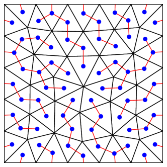
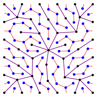
A possible realization of Example 2.2 on a two-dimensional grid is illustrated in Figure 1. Here, we have generated $\mathcal{T}_{1}^{*}$ by using a breadth-first search algorithm on the dual graph, rooted at the vertex $\nu_{0}$. From Figure 1, we observe that the space $P\Lambda^{1}$ can be decomposed in degrees of freedom associated with a map to the cells (the divergence), and a mapping from the nodes (rot). This observation is made more precise in the remainder of this section.

Lemma 2.3.

The decomposition from Example 2.2 is $p$-permitting (Definition 2.1).

Proof.

We need to show that $\mathring{\pi}\bar{d}:\bar{P}\Lambda^{k}\to\mathring{P}\Lambda^{k+1}$ is invertible for each $k$. Since $\bar{P}\Lambda^{n}$ is zero in this example, we are left with three non-trivial cases to consider:

  • $k=0$. In this case, the operator $\mathring{\pi}\bar{d}$ maps from the nodes to the edges of the spanning tree $\mathcal{T}_{1}$. Let $|\Delta_{0}|$ be the number of nodes in $\Omega_{h}$, then $\dim(\bar{P}\Lambda^{0})=|\Delta_{0}|-1$ since its functions have zero mean. Similarly, the number of edges on the tree is $|\Delta_{0}|-1$ and so $\dim(\bar{P}\Lambda^{0})=\dim(\mathring{P}\Lambda^{1})$.

    The operator $\mathring{\pi}\bar{d}$ can thus be represented as a square matrix and it remains to show that it is injective. Let $\bar{u}\in\bar{P}\Lambda^{0}$ satisfy $\mathring{\pi}\bar{d}\bar{u}=0$. This implies that the difference between each node connected by the tree $\mathcal{T}_{1}$ is zero. Since $\mathcal{T}_{1}$ is a spanning tree, this means that $\bar{u}$ is constant. The only constant in $P\Lambda^{0}$ is zero, so $\mathring{\pi}\bar{d}$ is injective.

  • $k=n-1$. Again, we first look at the dimensions of $\bar{P}\Lambda^{n-1}$ and $\mathring{P}\Lambda^{n}$. Let $|\Delta_{n-1}|$ and $|\Delta_{n}|$ denote the number of facets and cells in $\Omega_{h}$, respectively. Recall that the facet set $\mathcal{F}_{n-1}$ corresponds to the edges of a spanning tree with $|\Delta_{n}|+1$ vertices, so it contains $|\Delta_{n}|$ facets. In turn, we have $\dim(\bar{P}\Lambda^{n-1})=|\Delta_{n}|$. Since $\mathring{P}\Lambda^{n}=P\Lambda^{n}$, we also have $\dim(P\Lambda^{n})=|\Delta_{n}|$.

    The domain and range of the linear operator $\mathring{\pi}\bar{d}$ therefore have the same dimension, and it remains to show injectivity. Let $\bar{u}\in\bar{P}\Lambda^{n-1}$ with $\mathring{\pi}\bar{d}\bar{u}=0$. Since $\mathring{P}\Lambda^{n}=P\Lambda^{n}$, this implies that $d\bar{u}=0$. Now consider the cells associated with the leaves of the spanning tree $\mathcal{T}_{n-1}^{*}$. On each of these cells, $d\bar{u}$ is determined by one degree of freedom of $\bar{u}$, which must therefore be zero. We may then prune the tree by removing these leaves and repeat the argument on the reduced tree. Iterating until we reach the root of the tree, we have $\bar{u}=0$.

  • $k=1$, $n=3$. For the dimensions of $\bar{P}\Lambda^{1}$ and $\mathring{P}\Lambda^{2}$, let $|\Delta_{1}|$ denote the number of edges in $\Omega_{h}$. Then $\dim(\bar{P}\Lambda^{1})=\dim(P\Lambda^{1})-\dim(\mathring{P}\Lambda^{1})=|\Delta_{1}|-(|\Delta_{0}|-1)$ from the case $k=0$ above. Similarly, we have $\dim(\mathring{P}\Lambda^{2})=\dim(P\Lambda^{2})-\dim(\bar{P}\Lambda^{2})=|\Delta_{2}|-|\Delta_{3}|$ from the case $k=n-1$.

    We now note that $\Omega_{h}$ tesselates a contractible domain, and therefore its Euler characteristic is one, i.e. $\chi(\Omega_{h})\coloneqq|\Delta_{0}|-|\Delta_{1}|+|\Delta_{2}|-|\Delta_{3}|=1$. This allows us to derive

    $\displaystyle\dim(\bar{P}\Lambda^{1})=|\Delta_{1}|-|\Delta_{0}|+1=|\Delta_{2}|-|\Delta_{3}|=\dim(\mathring{P}\Lambda^{2}).$

    It remains to show that $\mathring{\pi}\bar{d}$ is injective, so let $\bar{u}\in\bar{P}\Lambda^{1}$ satisfy $\mathring{\pi}\bar{d}\bar{u}=0$, and thus $d\bar{u}\in\bar{P}\Lambda^{2}$. By the calculation for $k=n-1$ above, we have that $\mathring{\pi}\bar{d}$ is invertible on $\bar{P}\Lambda^{2}$. Using this in combination with $dd=0$, we obtain

    $\displaystyle d\bar{u}=(\mathring{\pi}\bar{d})^{-1}(\mathring{\pi}\bar{d})d\bar{u}=0.$

    Now, by the exactness of $(P\Lambda^{\bullet},d)$, a $v\in P\Lambda^{0}$ exists such that $dv=\bar{u}$. Since $\bar{P}\Lambda^{0}=P\Lambda^{0}$, we derive $\mathring{\pi}\bar{d}v=\mathring{\pi}dv=\mathring{\pi}\bar{u}=0$. Moreover, $\mathring{\pi}\bar{d}$ is invertible on $\bar{P}\Lambda^{0}$, as shown above, and therefore $v=0$ and $\bar{u}=0$.

In summary, $\mathring{\pi}\bar{d}$ is invertible for all $k$ and so the decomposition from Example 2.2 is $p$-permitting. ∎

Example 2.4 (Hodge decomposition).

We may alternatively define $\mathring{P}\Lambda^{k}=dP\Lambda^{k-1}$ and $\bar{P}\Lambda^{k}$ as its $L^{2}$-orthogonal complement, i.e. $\bar{P}\Lambda^{k}\perp\mathring{P}\Lambda^{k}$. This is known as the Hodge decomposition [6, Sec. 4.2.2]. The subspaces are then endowed with the $L^{2}$-projection operators $\mathring{\pi}$ and $\bar{\pi}$. While a $p$-permitting decomposition, the construction of a basis for $\bar{P}\Lambda^{k}$ and $\mathring{P}\Lambda^{k}$ is not as straightforward as in Example 2.2. Moreover, the projection operators involve solving linear systems, which is more computationally demanding than applying restrictions. We therefore continue with Example 2.2 instead.

Example 2.5 (Virtual element methods).

The construction from Example 2.2 can be generalized to the case of mixed virtual element methods on polytopal grids [8]. The lowest-order spaces $V\Lambda^{k}$ have one degree of freedom for each $k$-dimensional polytope of the mesh and form an exact sequence $(V\Lambda^{\bullet},d)$, as was shown in [15, 13]. The arguments from Definition 2.1 transfer directly to this case with only one minor adjustment. The dual graph $\mathcal{G}_{n-1}^{*}$ becomes a multi-graph because it is possible for a pair of elements to share multiple facets. Nevertheless, spanning trees can be constructed also for multi-graphs and the decomposition follows in the same manner.

2.2. The Poincaré operator

By the defining property of a $p$-permitting decomposition, we are able to invert the operator $\mathring{\pi}\bar{d}$ for each $k$. This allows us to construct the following operator.

Definition 2.6.

Let $P\Lambda^{\bullet}=\bar{P}\Lambda^{\bullet}\oplus\mathring{P}\Lambda^{\bullet}$ be a $p$-permitting decomposition of $(P\Lambda^{\bullet},d)$. The permitted operator $p:P\Lambda^{k}\to P\Lambda^{k-1}$ is given by

(2.3) $\displaystyle p\coloneqq(\mathring{\pi}\bar{d})^{-1}\mathring{\pi}.$

We are now ready to prove the main result of this work, namely that the permitted operator is a Poincaré operator (cf. Definition 1.1).

Theorem 2.7.

The permitted operator $p$ from Definition 2.6 is a Poincaré operator for $(P\Lambda^{\bullet},d)$, i.e. it satisfies

(2.4) $\displaystyle dp+pd=I.$
Proof.

Let $u\in P\Lambda^{k}$ be decomposed as $u=\bar{u}+\mathring{u}$ with $(\bar{u},\mathring{u})\in\bar{P}\Lambda^{k}\times\mathring{P}\Lambda^{k}$. Starting with $\bar{u}$, we note that $\mathring{\pi}\bar{u}=0$ and thus $p\bar{u}=0$. This allows us to derive:

(2.5) $\displaystyle(dp+pd)\bar{u}$ $\displaystyle=0+((\mathring{\pi}\bar{d})^{-1}\mathring{\pi})d\bar{u}=(\mathring{\pi}\bar{d})^{-1}(\mathring{\pi}\bar{d})\bar{u}=\bar{u}.$

Next, we consider the component $\mathring{u}$, for which we decompose the expression as

(2.6) $\displaystyle(dp+pd)\mathring{u}$ $\displaystyle=[\mathring{\pi}(dp+pd)\mathring{u}]+[\bar{\pi}(dp+pd)\mathring{u}].$

Let us first focus on the right-hand side term contained in $\mathring{P}\Lambda^{k}$. Since $p$ maps to $\bar{P}\Lambda^{k-1}$, we have $\mathring{\pi}p=0$ and thus:

(2.7) $\displaystyle\mathring{\pi}(dp+pd)\mathring{u}=\mathring{\pi}\bar{d}p\mathring{u}+0$ $\displaystyle=\mathring{\pi}\bar{d}(\mathring{\pi}\bar{d})^{-1}\mathring{\pi}\mathring{u}=\mathring{u}.$

It remains to consider the second term on the right-hand side of (2.6). For that, we note that $p$ is the composition of two surjective operators, and is therefore surjective onto $\bar{P}\Lambda^{k}$, i.e.

(2.8) $\displaystyle\operatorname{Ran}(p,P\Lambda^{k+1})=\bar{P}\Lambda^{k}.$

In turn, a $\mathring{t}\in\mathring{P}\Lambda^{k+1}$ exists such that $p\mathring{t}=\bar{\pi}dp\mathring{u}$. We find $\mathring{t}$ by applying the left-inverse operator $\mathring{\pi}\bar{d}:\bar{P}\Lambda^{k}\to\mathring{P}\Lambda^{k+1}$:

$\displaystyle\mathring{t}$ $\displaystyle=\mathring{\pi}\bar{d}\bar{\pi}d(\mathring{\pi}\bar{d})^{-1}\mathring{u}$
$\displaystyle=\mathring{\pi}d(I-\mathring{\pi})d(\mathring{\pi}\bar{d})^{-1}\mathring{u}$
$\displaystyle=0-\mathring{\pi}d(\mathring{\pi}\bar{d})(\mathring{\pi}\bar{d})^{-1}\mathring{u}=-\mathring{\pi}d\mathring{u}.$

It follows that $\bar{\pi}dp\mathring{u}=p\mathring{t}=-pd\mathring{u}$ and so

(2.9) $\displaystyle\bar{\pi}(dp+pd)\mathring{u}=-\bar{\pi}pd\mathring{u}+\bar{\pi}pd\mathring{u}=0.$

The combination of (2.5), (2.7), and (2.9) yields the result. ∎

Theorem 2.7 immediately provides several key results. First, we note that the operator $p$ induces its own exact sequence.

Lemma 2.8.

Let $p$ be the permitted operator from Definition 2.6. Then $(P\Lambda^{\bullet},p)$ is an exact sequence of negative grade, i.e.

(2.10) $\displaystyle\operatorname{Ran}(p,P\Lambda^{k+1})$ $\displaystyle=\operatorname{Ker}(p,P\Lambda^{k}),$

for each $k$.

Proof.

We start with the inclusion “$\subseteq$”. By (2.8), we have $\operatorname{Ran}(p,P\Lambda^{k+1})=\bar{P}\Lambda^{k}$. For $\bar{u}\in\bar{P}\Lambda^{k}$, we note that $p\bar{u}=0$ because $\mathring{\pi}\bar{u}=0$, and thus $\bar{u}\in\operatorname{Ker}(p,P\Lambda^{k})$. To prove the inclusion “$\supseteq$”, we consider $u\in P\Lambda^{k}$ with $pu=0$ and use Theorem 2.7 to derive $u=dpu+pdu=pdu$, so $u\in\operatorname{Ran}(p,P\Lambda^{k+1})$. ∎

Remark 2.9.

While $pp=0$ is valid for our construction, we note that any Poincaré operator can be modified to have this property by following [14, Thm. 5].

Secondly, Theorem 2.7 allows us to impose an alternative norm on $\bar{P}\Lambda^{k}$, with which we can formulate a simple, but well-posed, elliptic problem.

Lemma 2.10.

$\|\bar{u}\|_{\bar{P}\Lambda^{k}}\coloneqq\|d\bar{u}\|_{\Omega}$ is a norm on $\bar{P}\Lambda^{k}$.

Proof.

$\|\cdot\|_{\bar{P}\Lambda^{k}}$ is a semi-norm because $\|\cdot\|_{\Omega}$ is a norm and $d$ a linear operator. Now consider $\bar{u}\in\bar{P}\Lambda^{k}$ with $d\bar{u}=0$. By (2.8) and Lemma 2.8, we have $\bar{u}\in\operatorname{Ker}(p,P\Lambda^{k})$. Using Theorem 2.7, we derive

$\displaystyle\bar{u}=dp\bar{u}+pd\bar{u}=0.$

Corollary 2.11.

For given functional $\bar{f}\in(\bar{P}\Lambda^{k})^{*}$, the following problem is well-posed: find $\bar{u}\in\bar{P}\Lambda^{k}$ such that

(2.11) $\displaystyle(d\bar{u},d\bar{u}^{\prime})_{\Omega}$ $\displaystyle=\langle\bar{f},\bar{u}^{\prime}\rangle,$ $\displaystyle\forall\bar{u}^{\prime}$ $\displaystyle\in\bar{P}\Lambda^{k}.$
Proof.

The bilinear form $a(\bar{u},\bar{u}^{\prime})\coloneqq(d\bar{u},d\bar{u}^{\prime})_{\Omega}$ is continuous and coercive in $\|d\bar{u}\|_{\Omega}$, which is a norm on $\bar{P}\Lambda^{k}$ by Lemma 2.10. The result now follows by the Lax-Milgram theorem [9, Thm. 4.1.6]. ∎

Finally, the results of this section culminate to a new decomposition of the complex, described in the following theorem.

Theorem 2.12.

Given a $p$-permitting decomposition of $(P\Lambda^{\bullet},d)$, then each $P\Lambda^{k}$ decomposes as

(2.12) $\displaystyle P\Lambda^{k}=\bar{P}\Lambda^{k}\oplus d\bar{P}\Lambda^{k-1}.$
Proof.

The inclusion “$\supseteq$” is immediate. For “$\subseteq$”, let $u\in P\Lambda^{k}$ and consider $\bar{u}\coloneqq pdu\in\bar{P}\Lambda^{k}$ and $\bar{v}\coloneqq pu\in\bar{P}\Lambda^{k-1}$. Using Theorem 2.7, we derive

$\displaystyle\bar{u}+d\bar{v}=pdu+dpu=u.$

It remains to show that $\bar{P}\Lambda^{k}\cap d\bar{P}\Lambda^{k-1}=\{0\}$. For that, we consider $\bar{u}\in\bar{P}\Lambda^{k}$ that satisfies $\bar{u}=d\bar{v}$ for some $\bar{v}\in\bar{P}\Lambda^{k-1}$. We now calculate $\|\bar{u}\|_{\bar{P}\Lambda^{k}}=\|d\bar{u}\|_{\Omega}=\|dd\bar{v}\|_{\Omega}=0$, so $\bar{u}=0$ by Lemma 2.10. ∎

Remark 2.13.

We emphasize that the decomposition in Theorem 2.12 is not the same as the $p$-permitting $P\Lambda^{k}=\bar{P}\Lambda^{k}\oplus\mathring{P}\Lambda^{k}$ since $\mathring{P}\Lambda^{k}$ is not the same as $d\bar{P}\Lambda^{k-1}$ in general. Interestingly, the definitions do coincide in the special case of the Hodge decomposition in Example 2.4.

2.3. Poincaré constants

We now briefly turn our focus to the norm from Lemma 2.10. Although all norms are equivalent on the finite-dimensional space $\bar{P}\Lambda^{k}$, we pay attention to the constant with which this norm is stronger than the $L^{2}(\Omega)$ norm. We refer to it as the Poincaré constant on $\bar{P}\Lambda^{k}$, defined as follows.

Definition 2.14.

Let the Poincaré constant on $\bar{P}\Lambda^{k}$ be given by

(2.13) $\displaystyle\bar{c}_{k}\coloneqq\sup_{\bar{u}\in\bar{P}\Lambda^{k}}\frac{\|\bar{u}\|_{\Omega}}{\|d\bar{u}\|_{\Omega}}.$

The constant $\bar{c}_{k}$ plays an interesting role with respect to the full spaces $P\Lambda^{k}$. In particular, it provides an upper bound for the Poincaré constant on $P\Lambda^{k}$ and, in turn, can be used to bound the inf-sup constant for the pair $P\Lambda^{k-1}\times P\Lambda^{k}$ from below.

Lemma 2.15.

The Poincaré constant on $\bar{P}\Lambda^{k}$ forms an upper bound on the Poincaré constant on $P\Lambda^{k}$ (cf. [6, Sec. 4.2.3]). In particular, it holds that

(2.14) $\displaystyle\|u\|_{\Omega}$ $\displaystyle\leq\bar{c}_{k}\|du\|_{\Omega},$

for all $u\in P\Lambda^{k}$ with $u\perp\operatorname{Ker}(d,P\Lambda^{k})$.

Proof.

Let $u\in P\Lambda^{k}$ with $u\perp\operatorname{Ker}(d,P\Lambda^{k})$. We then obtain

$\displaystyle\|u\|_{\Omega}^{2}=(u,dpu+pdu)_{\Omega}=(u,pdu)_{\Omega}\leq\|u\|_{\Omega}\|pdu\|_{\Omega}.$

Using this bound, we proceed as follows

$\displaystyle\sup_{\begin{subarray}{c}u\in P\Lambda^{k}\\ u\perp\operatorname{Ker}(d,P\Lambda^{k})\end{subarray}}\frac{\|u\|_{\Omega}}{\|du\|_{\Omega}}$ $\displaystyle\leq\sup_{\begin{subarray}{c}u\in P\Lambda^{k}\\ u\perp\operatorname{Ker}(d,P\Lambda^{k})\end{subarray}}\frac{\|pdu\|_{\Omega}}{\|du\|_{\Omega}}$
(2.15) $\displaystyle=\sup_{u^{\prime}\in P\Lambda^{k}}\frac{\|pdu^{\prime}\|_{\Omega}}{\|du^{\prime}\|_{\Omega}}=\sup_{u^{\prime}\in P\Lambda^{k}}\frac{\|pdu^{\prime}\|_{\Omega}}{\|dpdu^{\prime}\|_{\Omega}}=\sup_{\bar{u}\in\bar{P}\Lambda^{k}}\frac{\|\bar{u}\|_{\Omega}}{\|d\bar{u}\|_{\Omega}}=\bar{c}_{k}.$

Where we used (1.3) and the fact that $pd$ is a projection, and thereby surjective. ∎

Remark 2.16.

From the calculation (2.3), we moreover see that $\bar{c}_{k}$ forms a lower bound on the continuity constant of $p_{k+1}$. Namely,

$\displaystyle\bar{c}_{k}=\sup_{u^{\prime}\in P\Lambda^{k}}\frac{\|pdu^{\prime}\|_{\Omega}}{\|du^{\prime}\|_{\Omega}}\leq\sup_{u^{\prime}\in P\Lambda^{k}}\frac{\|pdu^{\prime}\|_{H\Lambda^{k}}}{\|du^{\prime}\|_{H\Lambda^{k+1}}}\leq\sup_{t\in P\Lambda^{k+1}}\frac{\|pt\|_{H\Lambda^{k}}}{\|t\|_{H\Lambda^{k+1}}}\eqqcolon\|p_{k+1}\|,$

with the $H\Lambda^{k}$-norm defined in (1.4). While of limited practical value, this indicates that $\bar{c}_{k}$ may form a sharper estimate than $\|p_{k+1}\|$ for the Poincaré constant on $P\Lambda^{k}$.

Corollary 2.17.

The inf-sup constant for the pair $P\Lambda^{k-1}\times P\Lambda^{k}$ is bounded from below as

(2.16) $\displaystyle\inf_{\begin{subarray}{c}u\in P\Lambda^{k}\\ du=0\end{subarray}}\sup_{v\in P\Lambda^{k-1}}\frac{(dv,u)_{\Omega}}{\|v\|_{H\Lambda^{k-1}}\|u\|_{H\Lambda^{k}}}\geq\frac{1}{\sqrt{\bar{c}_{k-1}^{2}+1}}.$
Proof.

By the exact sequence property, we have $u\in\operatorname{Ker}(d,P\Lambda^{k})=\operatorname{Ran}(d,P\Lambda^{k-1})$. We may therefore equivalently take the infimum over $v^{\prime}\in P\Lambda^{k-1}$ with $v^{\prime}\perp\operatorname{Ker}(d,P\Lambda^{k-1})$. We derive by choosing $v=v^{\prime}$ that

$\displaystyle\inf_{\begin{subarray}{c}v^{\prime}\in P\Lambda^{k-1}\\ v^{\prime}\perp\operatorname{Ker}(d,P\Lambda^{k-1})\end{subarray}}\sup_{v\in P\Lambda^{k-1}}\frac{(dv,dv^{\prime})_{\Omega}}{\|v\|_{H\Lambda^{k-1}}\|dv^{\prime}\|_{H\Lambda^{k}}}$ $\displaystyle\geq\inf_{\begin{subarray}{c}v^{\prime}\in P\Lambda^{k-1}\\ v^{\prime}\perp\operatorname{Ker}(d,P\Lambda^{k-1})\end{subarray}}\frac{\|dv^{\prime}\|_{\Omega}}{\|v^{\prime}\|_{H\Lambda^{k-1}}}.$

Lemma 2.15 provides the bound $\|v^{\prime}\|_{H\Lambda^{k-1}}^{2}\leq(\bar{c}_{k-1}^{2}+1)\|dv^{\prime}\|_{\Omega}^{2}$, which concludes the proof. ∎

3. A solver for the Hodge-Laplace problem

In this section, we focus on the discretization of the Hodge-Laplace problem (1.5). For ease of reference, we state the discrete problem: for given functionals $g\in(P\Lambda^{k-1})^{*}$ and $f\in(P\Lambda^{k})^{*}$, find $(v,u)\in P\Lambda^{k-1}\times P\Lambda^{k}$ such that

(3.1a) $\displaystyle(v,v^{\prime})_{\Omega}-(u,dv^{\prime})_{\Omega}$ $\displaystyle=\langle g,v^{\prime}\rangle,$ $\displaystyle\forall v^{\prime}$ $\displaystyle\in P\Lambda^{k-1},$
(3.1b) $\displaystyle(dv,u^{\prime})_{\Omega}+(du,du^{\prime})_{\Omega}$ $\displaystyle=\langle f,u^{\prime}\rangle,$ $\displaystyle\forall u^{\prime}$ $\displaystyle\in P\Lambda^{k}.$

We now use the results from the previous section to create a practical method that solves (3.1). In particular, Theorem 2.12 allows us to decompose the test and trial functions in (3.1) in components from the spaces $\bar{P}\Lambda^{\bullet}$. This effectively splits the Hodge-Laplace problem into four smaller problems, that can be solved sequentially:

  • Find $\bar{v}\in\bar{P}\Lambda^{k-1}$ such that

    (3.2a) $\displaystyle(d\bar{v},d\bar{v}^{\prime})_{\Omega}$ $\displaystyle=\langle f,d\bar{v}^{\prime}\rangle,$ $\displaystyle\forall\bar{v}^{\prime}$ $\displaystyle\in\bar{P}\Lambda^{k-1}.$
    (3.2b) $\displaystyle(d\bar{w}_{v},d\bar{w}^{\prime})_{\Omega}$ $\displaystyle=\langle g,d\bar{w}^{\prime}\rangle-(\bar{v},d\bar{w}^{\prime})_{\Omega},$ $\displaystyle\forall\bar{w}^{\prime}$ $\displaystyle\in\bar{P}\Lambda^{k-2}.$
    (3.2c) $\displaystyle(d\bar{u},d\bar{u}^{\prime})_{\Omega}$ $\displaystyle=\langle f,\bar{u}^{\prime}\rangle-(d\bar{v},\bar{u}^{\prime})_{\Omega},$ $\displaystyle\forall\bar{u}^{\prime}$ $\displaystyle\in\bar{P}\Lambda^{k}.$
    (3.2d) $\displaystyle(d\bar{v}_{u},d\bar{v}^{\prime})_{\Omega}$ $\displaystyle=(\bar{v}+d\bar{w}_{v},\bar{v}^{\prime})_{\Omega}-(\bar{u},d\bar{v}^{\prime})_{\Omega}-\langle g,\bar{v}^{\prime}\rangle,$ $\displaystyle\forall\bar{v}^{\prime}$ $\displaystyle\in\bar{P}\Lambda^{k-1}.$

Finally, we collect the solutions from the four problems and set:

(3.2e) $\displaystyle v$ $\displaystyle\coloneqq\bar{v}+d\bar{w}_{v},$ $\displaystyle u$ $\displaystyle\coloneqq\bar{u}+d\bar{v}_{u}.$

We emphasize that each of the sub-problems is well-posed by Corollary 2.11. In turn, (3.2) is a direct solver for (3.1) and confirms existence of a solution, as shown in the following lemma.

Lemma 3.1.

The pair $(v,u)\in P\Lambda^{k-1}\times P\Lambda^{k}$ from (3.2e) is the solution to the Hodge-Laplace problem (3.1).

Proof.

First, (3.2b) and (3.2d) give us

$\displaystyle(v,d\bar{w}^{\prime})_{\Omega}$ $\displaystyle=\langle g,d\bar{w}^{\prime}\rangle,$ $\displaystyle\forall\bar{w}^{\prime}$ $\displaystyle\in\bar{P}\Lambda^{k-2},$
$\displaystyle(v,\bar{v}^{\prime})_{\Omega}-(u,d\bar{v}^{\prime})_{\Omega}$ $\displaystyle=\langle g,\bar{v}^{\prime}\rangle,$ $\displaystyle\forall\bar{v}^{\prime}$ $\displaystyle\in\bar{P}\Lambda^{k-1}.$

Next, Theorem 2.12 allows us to decompose the test function $v^{\prime}\in P\Lambda^{k-1}$ as $v^{\prime}=\bar{v}^{\prime}+d\bar{w}^{\prime}$ with $(\bar{v}^{\prime},\bar{w}^{\prime})\in\bar{P}\Lambda^{k-1}\times\bar{P}\Lambda^{k-2}$. Using the fact that $dd\bar{w}^{\prime}=0$, we obtain

$\displaystyle(v,v^{\prime})_{\Omega}-(u,dv^{\prime})_{\Omega}$ $\displaystyle=(v,\bar{v}^{\prime}+d\bar{w}^{\prime})_{\Omega}-(u,d\bar{v}^{\prime})_{\Omega}$
$\displaystyle=\langle g,\bar{v}^{\prime}+d\bar{w}^{\prime}\rangle=\langle g,v^{\prime}\rangle,$ $\displaystyle\forall v^{\prime}$ $\displaystyle\in P\Lambda^{k-1}$

Similarly, (3.2a) and (3.2c) give us

$\displaystyle(dv,d\bar{v}^{\prime})_{\Omega}$ $\displaystyle=\langle f,d\bar{v}^{\prime}\rangle,$ $\displaystyle\forall\bar{v}^{\prime}$ $\displaystyle\in\bar{P}\Lambda^{k-1},$
$\displaystyle(dv,\bar{u}^{\prime})_{\Omega}+(du,d\bar{u}^{\prime})_{\Omega}$ $\displaystyle=\langle f,\bar{u}^{\prime}\rangle,$ $\displaystyle\forall\bar{u}^{\prime}$ $\displaystyle\in\bar{P}\Lambda^{k}.$

Thus, if we decompose $u^{\prime}\in P\Lambda^{k}$ as $u^{\prime}=\bar{u}^{\prime}+d\bar{v}^{\prime}$ with $(\bar{u}^{\prime},\bar{v}^{\prime})\in\bar{P}\Lambda^{k}\times\bar{P}\Lambda^{k-1}$, we obtain

$\displaystyle(dv,u^{\prime})_{\Omega}+(du,du^{\prime})_{\Omega}$ $\displaystyle=(dv,\bar{u}^{\prime}+d\bar{v}^{\prime})_{\Omega}+(du,d\bar{u}^{\prime})_{\Omega}$
$\displaystyle=\langle f,\bar{u}^{\prime}+d\bar{v}^{\prime}\rangle=\langle f,u^{\prime}\rangle,$ $\displaystyle\forall u^{\prime}$ $\displaystyle\in P\Lambda^{k}$

In conclusion, $(v,u)$ is the solution to (3.1). ∎

Observe that each of the problems in (3.2) is significantly smaller than the original problem (3.1). This is because Theorem 2.12 defines a different basis for the space $P\Lambda^{k}$ and (3.2) is simply (3.1) expressed in that basis. This observation is emphasized in the next lemma, for which we introduce the short-hand notation

(3.3) $\displaystyle n_{k}$ $\displaystyle\coloneqq\dim(P\Lambda^{k}),$ $\displaystyle\bar{n}_{k}$ $\displaystyle\coloneqq\dim(\bar{P}\Lambda^{k}),$ $\displaystyle\mathring{n}_{k}$ $\displaystyle\coloneqq\dim(\mathring{P}\Lambda^{k}).$
Lemma 3.2.

The dimension of the original Hodge-Laplace problem (3.1) is equal to the sum of dimensions of the four subproblems (3.2).

Proof.

The operator $\mathring{\pi}\bar{d}:\bar{P}\Lambda^{k}\to\mathring{P}\Lambda^{k+1}$ is invertible by Definition 2.1, so the dimensions of its domain and range coincide, i.e. $\bar{n}_{k}=\mathring{n}_{k+1}$ for all $k$. In turn, we obtain $n_{k-1}=\bar{n}_{k-1}+\mathring{n}_{k-1}=\bar{n}_{k-1}+\bar{n}_{k-2}$ and similarly $n_{k}=\bar{n}_{k}+\bar{n}_{k-1}$. ∎

Remark 3.3.

In practical applications, $v\in P\Lambda^{k-1}$ is often the variable of interest whereas $u\in P\Lambda^{k}$ is merely an auxiliary variable or a Lagrange multiplier. The calculation from Lemma 3.2 shows that we obtain $v$ by solving two symmetric positive definite problems of total size $n_{k-1}$ instead of the original saddle point system of size $n_{k-1}+n_{k}$.

For example, Darcy flow in porous media can be modeled by (3.1) with $k=n$, in which $v$ denotes the fluid flux, $u$ the pressure, and $d$ the divergence. If the flux is the important variable, e.g. when modeling contaminant transport, then the procedure (3.2) is particularly attractive because it is obtained from the first two problems, (3.2a) and (3.2b).

Remark 3.4 (The case $k=n$).

Since $d_{n}=0$ and $d_{n-1}$ is surjective, the procedure from (3.2) simplifies to the following three problems.

  • Find $\bar{v}\in\bar{P}\Lambda^{n-1}$ such that

    (3.4a) $\displaystyle(d\bar{v},u^{\prime})_{\Omega}$ $\displaystyle=\langle f,u^{\prime}\rangle,$ $\displaystyle\forall u^{\prime}$ $\displaystyle\in P\Lambda^{n}.$
    (3.4b) $\displaystyle(d\bar{w}_{v},d\bar{w}^{\prime})_{\Omega}$ $\displaystyle=\langle g,d\bar{w}^{\prime}\rangle-(\bar{v},d\bar{w}^{\prime})_{\Omega},$ $\displaystyle\forall\bar{w}^{\prime}$ $\displaystyle\in\bar{P}\Lambda^{n-2}.$
    (3.4c) $\displaystyle(u,d\bar{v}^{\prime})_{\Omega}$ $\displaystyle=(\bar{v}+d\bar{w}_{v},\bar{v}^{\prime})_{\Omega}-\langle g,\bar{v}^{\prime}\rangle,$ $\displaystyle\forall\bar{v}^{\prime}$ $\displaystyle\in\bar{P}\Lambda^{n-1}.$

Finally, we set $v=\bar{v}+d\bar{w}_{v}$.

In the case of Example 2.2, (3.4a) and (3.4c) are sparse, triangular systems due to the underlying tree structure, as observed in [10]. These can therefore be solved in linear time with respect to the number of elements. The remaining subproblem (3.4b) is a symmetric, positive definite system of size $\bar{n}_{n-2}$, which corresponds to the number of faces minus the number of cells.

Note that (3.4b) is exactly (3.1a) posed in a divergence-free subspace of $P\Lambda^{n-1}$. Divergence-free finite element spaces for this problem were proposed in [3, 16], which are examples of the form $d\bar{P}\Lambda^{n-2}$. In particular, they correspond to the curl of a subset of the $H(\operatorname{curl})$-conforming elements $P\Lambda^{n-2}$, filtered by a spanning tree.

As shown in Lemma 3.1, the true solution is found by (3.2) if exact solvers are used. However, it may be advantageous to use inexact, iterative solvers in some of the steps. As shown in Corollary 2.11, the problems (3.2) are symmetric and positive definite, and thus amenable to efficient solvers such as the Conjugate Gradient method. We highlight an important implication of such solvers in the following lemma.

Lemma 3.5.

If inexact solvers are used in (3.2), then the error in (3.1b) depends only on the accuracy at which (3.2a) and (3.2c) are solved.

Proof.

Let $(v_{*},u_{*})\in P\Lambda^{k-1}\times P\Lambda^{k}$ be the solution obtained using inexact solvers with $v_{*}=\bar{v}_{*}+d\bar{w}_{v,*}$ and $u_{*}=\bar{u}_{*}+d\bar{v}_{u,*}$. The error equation for (3.1b) becomes

$\displaystyle(dv_{*},u^{\prime})_{\Omega}+(du_{*},du^{\prime})_{\Omega}-\langle f,u^{\prime}\rangle$ $\displaystyle=(d\bar{v}_{*},u^{\prime})_{\Omega}+(d\bar{u}_{*},du^{\prime})_{\Omega}-\langle f,u^{\prime}\rangle.$

In other words, the error only depends on the components $(\bar{v}_{*},\bar{u}_{*})$, which are obtained from (3.2a) and (3.2c). ∎

4. Auxiliary space preconditioning for elliptic problems

The solver proposed in Section 3 depends on the particular structure of the Hodge-Laplace problem and uses it to its advantage. In this section, we aim to exploit the results from Section 2 in a different way that is applicable to a more general class of problems.

For that, we use the framework of norm-equivalent preconditioning [20], which argues that the canonical preconditioner for elliptic finite element problems is given by the Riesz representation operator. In short, if the problem is well-posed in a certain, parameter-weighted norm, then that norm determines a suitable preconditioner. Such a norm is often a weighted variant of the $H\Lambda^{k}$ norm from (1.4) so let us consider

(4.1) $\displaystyle\|u\|_{U}^{2}\coloneqq\|\alpha u\|_{\Omega}^{2}+\|du\|_{\Omega}^{2}.$

in which $0<\alpha\leq 1$ is a fixed constant. Following [20], if our problem is well-posed in this norm, then the canonical preconditioner involves solving the following projection problem: given $f\in(P\Lambda^{k})^{*}$, find $u\in P\Lambda^{k}$ such that

(4.2) $\displaystyle(\alpha^{2}u,u^{\prime})_{\Omega}+(du,du^{\prime})_{\Omega}$ $\displaystyle=\langle f,u^{\prime}\rangle,$ $\displaystyle\forall u^{\prime}$ $\displaystyle\in P\Lambda^{k}.$

However, problem (4.2) may be challenging to solve numerically if $\alpha$ is small, because the term $(du,du^{\prime})_{\Omega}$ has a large kernel for $0<k<n$. To handle this, we follow the framework of [18] and construct an auxiliary space preconditioner based on the decomposition from Theorem 2.12. In particular, we define the auxiliary spaces $U_{j}$ and transfer operators $\Pi_{j}:U_{j}\to P\Lambda^{k}$ as

(4.3a) $\displaystyle U_{1}$ $\displaystyle\coloneqq\bar{P}\Lambda^{k},$ $\displaystyle\|\bar{u}\|_{U_{1}}$ $\displaystyle\coloneqq\|d\bar{u}\|_{\Omega},$ $\displaystyle\Pi_{1}\bar{u}$ $\displaystyle\coloneqq\bar{u},$
(4.3b) $\displaystyle U_{2}$ $\displaystyle\coloneqq\bar{P}\Lambda^{k-1},$ $\displaystyle\|\bar{v}\|_{U_{2}}$ $\displaystyle\coloneqq\|\alpha d\bar{v}\|_{\Omega},$ $\displaystyle\Pi_{2}\bar{v}$ $\displaystyle\coloneqq d\bar{v}.$

Next, we show two stability results, concerning first the transfer operators and second, the decomposition.

Lemma 4.1.

The transfer operators $\Pi_{j}$ from (4.3) are stable. I.e. for each $j\in\{1,2\}$, a bounded $c_{j}\in\mathbb{R}$ exists such that

(4.4) $\displaystyle\|\Pi_{j}u_{j}\|_{U}$ $\displaystyle\leq c_{j}\|u_{j}\|_{U_{j}},$ $\displaystyle\forall u_{j}$ $\displaystyle\in U_{j},$

where $c_{j}$ may depend on $\bar{c}_{k}$ from Definition 2.14, but not on $\alpha$.

Proof.

The result follows immediately from Definition 2.14, the upper bound on $\alpha$, and the identity $dd=0$:

(4.5a) $\displaystyle\|\alpha\bar{u}\|_{\Omega}^{2}+\|d\bar{u}\|_{\Omega}^{2}$ $\displaystyle\leq((\alpha\bar{c}_{k})^{2}+1)\|d\bar{u}\|_{\Omega}^{2}\leq(\bar{c}_{k}^{2}+1)\|d\bar{u}\|_{\Omega}^{2},$ $\displaystyle\forall\bar{u}$ $\displaystyle\in\bar{P}\Lambda^{k},$
(4.5b) $\displaystyle\|\alpha d\bar{v}\|_{\Omega}^{2}+\|d(d\bar{v})\|_{\Omega}^{2}$ $\displaystyle=\|\alpha d\bar{v}\|_{\Omega}^{2},$ $\displaystyle\forall\bar{v}$ $\displaystyle\in\bar{P}\Lambda^{k-1}.$

Lemma 4.2.

The decomposition from Theorem 2.12 is stable in the norms from (4.1) and (4.3). In particular, if $u\in P\Lambda^{k}$ decomposes as $u=\bar{u}+d\bar{v}$ with $(\bar{u},\bar{v})\in\bar{P}\Lambda^{k}\times\bar{P}\Lambda^{k-1}$, then

(4.6) $\displaystyle\|d\bar{u}\|_{\Omega}^{2}+\|\alpha d\bar{v}\|_{\Omega}^{2}\leq 2\|\alpha u\|_{\Omega}^{2}+(1+2\bar{c}_{k}^{2})\|du\|_{\Omega}^{2}.$
Proof.

Recall from Theorem 2.12 that the decomposition is uniquely given by $\bar{u}=pdu$ and $\bar{v}=pu$. Using the identity (1.3), we derive

(4.7) $\displaystyle\|d\bar{u}\|_{\Omega}^{2}=\|dpdu\|_{\Omega}^{2}=\|du\|_{\Omega}^{2}.$

Next, we bound $\bar{v}$ by using the decomposition $d\bar{v}=u-\bar{u}$, Definition 2.14, and the upper bound on $\alpha$

$\displaystyle\|\alpha d\bar{v}\|_{\Omega}^{2}\leq 2\|\alpha u\|_{\Omega}^{2}+2\|\alpha\bar{u}\|_{\Omega}^{2}$ $\displaystyle\leq 2\|\alpha u\|_{\Omega}^{2}+2(\alpha\bar{c}_{k})^{2}\|d\bar{u}\|_{\Omega}^{2}$
(4.8) $\displaystyle\leq 2\|\alpha u\|_{\Omega}^{2}+2\bar{c}_{k}^{2}\|du\|_{\Omega}^{2}.$

Together, (4.7) and (4) yield the result. ∎

Let $\mathsf{\bar{\Pi}_{k}}\in\mathbb{R}^{\bar{n}_{k}\times n_{k}}$ be the matrix representation of the restriction operator $\bar{\pi}$ on $P\Lambda^{k}$. Similarly, let $\mathsf{\bar{D}_{k-1}}\in\mathbb{R}^{n_{k}\times\bar{n}_{k-1}}$ represent the differential $\bar{d}$ on $\bar{P}\Lambda^{k-1}$. Finally, let $\mathsf{\bar{A}_{k}}\in\mathbb{R}^{\bar{n}_{k}\times\bar{n}_{k}}$ be the Gram matrix for the norm from Lemma 2.10. In other words,

$\displaystyle\|d\bar{u}\|_{\Omega}^{2}$ $\displaystyle=\mathsf{\bar{u}^{T}\bar{A}_{k}\bar{u}},$ $\displaystyle\forall\bar{u}$ $\displaystyle\in\bar{P}\Lambda^{k},$

in which $\mathsf{\bar{u}}\in\mathbb{R}^{n_{k}}$ is the vector representation of $\bar{u}$. Using these ingredients, we now construct our preconditioner.

Definition 4.3.

The auxiliary space preconditioner for (4.2), based on the decomposition from Theorem 2.12, is given by

(4.9) $\displaystyle\mathsf{P\coloneqq\bar{\Pi}_{k}^{T}\bar{A}_{k}^{-1}\bar{\Pi}_{k}}+\mathsf{\bar{D}_{k-1}}(\alpha^{2}\mathsf{\bar{A}_{k-1})^{-1}\bar{D}_{k-1}^{T}}.$
Lemma 4.4.

The auxiliary space preconditioner $\mathsf{P}$ from Definition 4.3 is robust with respect to $0<\alpha\leq 1$. Moreover, if the Poincaré constant $\bar{c}_{k}$ is independent of the mesh size $h$, then $\mathsf{P}$ is robust with respect to $h$.

Proof.

We verify the assumptions of [18, Thm. 2.2]. First, Theorem 2.12 provides the decomposition and therefore the surjectivity of the combined transfer operators. The stability of these operators is shown in Lemma 4.1. Since there is no high-frequency term in this decomposition, we do not require a smoother. Finally, Lemma 4.2 provides the stability of the decomposition.

Next, we note that the bounds in these results are independent of $\alpha$ but may depend on $\bar{c}_{k}$. In turn, [18, Thm. 2.2] shows that the spectral condition number of the preconditioned system is independent of $\alpha$. Moreover, if $\bar{c}_{k}$ is independent of $h$, then the preconditioner is robust with respect to $h$ as well. ∎

5. Numerical results

We now present three numerical experiments that highlight the practical impact of the results derived in the previous sections. Section 5.1 concerns the four-step solution procedure from Section 3, Section 5.2 investigates the Poincaré constant from Section 2.3, and Section 5.3 considers the auxiliary space preconditioners from Section 4.

Throughout this section, we define $P\Lambda^{\bullet}$ as the Whitney forms from Example 1.2 and consider the $p$-permitting decomposition described in Example 2.2. We construct the spanning trees as follows. Let $\mathcal{T}_{n-1}^{*}$ be the spanning tree of the dual graph $\mathcal{G}_{n-1}^{*}$, obtained by a breadth-first search algorithm rooted at $\nu_{0}$, the vertex that corresponds to the “outside cell”. We note that this construction is similar to [19, Sec. 7.3]. Moreover, [2, Sec. 6] showed that a breadth-first is typically prefered over a depth-first search algorithm. If $n=2$, we define $\mathcal{E}_{1}$ as the complement to $\mathcal{F}_{1}$. An illustration in 2D is given in Figure 1. Finally, for $n=3$, we define $\mathcal{T}_{1}$ as the spanning tree of the nodes, using again a breadth-first search, rooted at the node that is closest to the center of the domain.

The code is written in Python 3, uses the package PyGeoN[12], and is available at github.com/wmboon/poincare.

5.1. Solving the Hodge-Laplace problem

In this section, we investigate the efficiency of the four-step solution procedure (3.2) proposed in Section 3.

The experimental set-up is as follows. Let $\Omega_{h}$ be an unstructured simplicial grid of the unit cube consisting of approximately $19\,000$ elements. The elements have mean diameter of $h\approx 0.1$. We set up the Hodge-Laplace problem with randomly chosen right-hand sides. We then compare the solution times needed for a direct solver for each of the sub-problems of (3.2) with the time required to solve the saddle-point system (3.1). For each problem, we report the number of degrees of freedom and the time required by a direct solver. The results are presented in Table 1.

Table 1. Dimensions and solution times of the four subproblems in (3.2) compared to the original system (3.1) on the unit cube.
$k=1$ $k=2$ $k=3$
Problem DoF Time DoF Time DoF Time
$\bar{P}\Lambda^{k-1}$ (3.2a) $4036$ 0.18s $20\,919$ 5.78s $19\,071$ 0.02s
$\bar{P}\Lambda^{k-2}$ (3.2b) 00 - $4036$ 0.18s $20\,919$ 5.65s
$\bar{P}\Lambda^{k}$ (3.2c) $20\,919$ 5.80s $19\,071$ 0.02s 00 -
$\bar{P}\Lambda^{k-1}$ (3.2d) $4036$ 0.19s $20\,919$ 5.67s $19\,071$ 0.02s
Total (3.2) $28\,992$ 6.17s $64\,945$ 11.65s $59\,061$ 5.69s
Original system (3.1) $28\,992$ 28.08s $64\,945$ 158.41s $59\,061$ 27.22s

First, while it is unsurprising that the total numbers of degrees of freedom coincide (cf. Lemma 3.2), it is noteworthy that the problem is decomposed into three subproblems of roughly equal size for $k=3$.

Second, we observe a speed-up factor of at least four for all instances of $k$, without loss of accuracy, indicating the potential of the approach. The best relative performance is seen in the case of $k=2$, i.e. the Hodge-Laplace problem posed on the Raviart-Thomas space, where the speed-up factor exceeds 10. Interestingly, this is the only problem that requires solving all three kinds of subproblems. We make two more observations regarding the efficiency in solving the subproblems. First, the problems posed on $\bar{P}\Lambda^{2}$ have an underlying tree structure which allows them to be solved in sequence, from the leaves to the root. We have not explicitly informed the solver of this and implemented exactly (3.2). Nonetheless, these problems are solved within two hundredths of a second. Second, the problems on $\bar{P}\Lambda^{0}$ are simply much smaller than the others because there are far fewer nodes than edges or faces in the grid. These problems are therefore also solved relatively quickly.

Third, we note that each of the (sub)problems can be solved with more efficient solution methods. However, we have opted for a standard, direct linear solver in all cases to keep the comparison relatively fair. The performance of different iterative solvers forms a study in its own right, which we reserve as a topic for future investigation.

Finally, assembly times were not included in this comparison. This is because the assembly of (3.2) is similar to the assembly of (3.1) because each term consists of the same building blocks. In particular, for given $k$ we require the mass matrices of $P\Lambda^{k-1}$, $P\Lambda^{k}$, and $P\Lambda^{k+1}$. The matrix representations of the differentials, $\mathsf{D}_{k}$, can directly be obtained from the incidence matrices of the mesh. All that remains is the restriction onto the subspaces $\bar{P}\Lambda^{k}$, which can be done using the same machinery as imposing essential boundary conditions. We emphasize that one can apply the solution procedure (3.2) without assembly of the original system (3.1). If direct solvers are used, as they are here, then the same solution is obtained, as was shown in Lemma 3.1.

5.2. Computing the Poincaré constant

To compute the constant from Definition 2.14, we consider the following generalized eigenvalue problem: find the largest $\lambda\in\mathbb{R}$ such that a $\bar{u}\in\bar{P}\Lambda^{k}$ exists with

(5.1) $\displaystyle(\bar{u},\bar{u}^{\prime})_{\Omega}$ $\displaystyle=\lambda(d\bar{u},d\bar{u}^{\prime})_{\Omega},$ $\displaystyle\forall\bar{u}^{\prime}\in\bar{P}\Lambda^{k}.$

It then follows that $\bar{c}_{k}=\sqrt{\lambda}$. We note that this problem can be handled numerically because the matrices on the left and right-hand sides are both invertible. This allows us to compute $\bar{c}_{k}$ for a series of meshes on the unit square and cube. We present the computed constants in Table 2. The mesh used in Section 5.1 corresponds to the finest level on the unit cube.

Table 2. Computed constants $\bar{c}_{k}$ (cf. Definition 2.14) on the unit square and cube. Lemma 2.15 shows that $\bar{c}_{k}$ forms an upper bound on the Poincaré constant of $P\Lambda^{k}$.
Unit square Unit cube
$h$ $k=0$ $k=1$ $h$ $k=0$ $k=1$ $k=2$
1.28e-01 3.17e-01 3.66e-01 9.02e-01 3.35e-01 9.04e-01 4.61e-01
6.42e-02 3.18e-01 4.36e-01 5.84e-01 3.03e-01 5.11e-01 5.75e-01
3.17e-02 3.18e-01 3.49e-01 3.79e-01 3.11e-01 8.01e-01 5.00e-01
1.57e-02 3.18e-01 3.48e-01 2.01e-01 3.16e-01 1.23e00 6.16e-01
7.83e-03 3.18e-01 3.33e-01 1.02e-01 3.18e-01 1.75e00 9.33e-01

The case $k=0$ provides the most stable constants because $\bar{P}\Lambda^{0}=P\Lambda^{0}=\mathbb{L}_{1}/\mathbb{R}$ (cf. Example 1.2). In turn, $\bar{c}_{0}$ is exactly the Poincaré constant for the gradient on the nodal space $P\Lambda^{0}$. For both cases of $n$, the constant approximates $1/\pi$.

The other constants are therefore of more interest. In the two-dimensional case, we observe that $\bar{c}_{1}$ is independent of the mesh size $h$. We provide an intuitive, albeit less rigorous, explanation for this. $\bar{P}\Lambda^{1}$ can be viewed as the subspace of $P\Lambda^{1}$ with homogeneous essential boundary conditions on $\mathcal{E}_{1}$ (the purple tree on the right of Figure 1). The domain is thus effectively cut into “ribbons” that each have width $h$ and a maximal length related to the diameter of the domain. In the limit, the Poincaré constant on each of these ribbons is dominated by its length, not its width.

In 3D, both $\bar{c}_{1}$ and $\bar{c}_{2}$ exhibit a mild increase with respect to $h$. However, this inverse dependency is sub-linear since $\bar{c}_{2}$ increases by a factor 2 for a mesh size that decreases by a factor 9. If we were to fit a power law on the finest meshes, we would obtain approximate rates of $\bar{c}_{k}\approx\mathcal{O}(h^{-0.5})$ in both cases. We emphasize that these are the constants that result from our specific choice of spanning trees. We therefore do not exclude the possibility of getting a better scaling with a different construction, or finer meshes.

5.3. Preconditioning the projection problem

The results from the previous experiment indicate that $\bar{c}_{k}$ is independent of $h$ in 2D and we may expect only a mild dependency of $h$ in 3D. We therefore continue by investigating whether this has an influence on the performance of the auxiliary space preconditioners proposed in Section 4.

We thus consider the projection problem (4.2) and note that the proposed preconditioner is only relevant for the cases $1\leq k\leq n-1$, leaving three non-trivial cases. Using the same grids as in the previous section, we investigate its performance for a range of $0<\alpha\leq 1$ by computing the spectral condition numbers of the preconditioned system. We moreover report the numbers of iterations required by the Minimal Residual Method (MinRes) to reach a relative residual of $10^{-8}$ for a random right-hand side $f$.

Table 3. Performance of the auxiliary space preconditioner proposed in Definition 4.3 for the projection problem (4.2). Condition numbers for the finest grids are omitted due to high computational costs.
Condition numbers MinRes iterations
$\log_{10}(\alpha)$ -4 -3 -2 -1 0 -4 -3 -2 -1 0
$h$ Unit square, $k=1$
1.28e-01 1.00 1.00 1.01 1.07 2.03 1 1 2 3 10
6.42e-02 1.00 1.00 1.01 1.09 2.33 1 1 1 3 9
3.17e-02 1.00 1.00 1.01 1.07 1.99 1 1 1 3 8
1.57e-02 1.00 1.00 1.01 1.07 1.99 1 1 1 3 8
7.83e-03 - - - - - 1 1 1 2 7
$h$ Unit cube, $k=1$
9.02e-01 1.00 1.00 1.02 1.19 5.55 1 1 2 4 15
5.84e-01 1.00 1.00 1.01 1.11 2.69 1 1 1 3 10
3.79e-01 1.00 1.00 1.02 1.17 4.72 1 1 1 3 13
2.01e-01 1.00 1.00 1.04 1.28 10.17 1 1 1 3 15
1.02e-01 - - - - - 1 1 1 2 18
$h$ Unit cube, $k=2$
9.02e-01 1.00 1.00 1.01 1.09 2.40 1 1 2 4 11
5.84e-01 1.00 1.00 1.01 1.12 3.02 1 1 2 4 12
3.79e-01 1.00 1.00 1.01 1.10 2.63 1 1 2 3 11
2.01e-01 1.00 1.00 1.02 1.13 3.34 1 1 1 3 12
1.02e-01 - - - - - 1 1 1 3 15

As shown in Table 3, the preconditioner is particularly effective for small values of $\alpha$, often letting MinRes converge in one iteration. This is remarkable because in that case, the second term in (4.2) dominates which has a large kernel. The small $\alpha$ case is therefore typically more challenging to handle but our approach, based on the decomposition from Theorem 2.12, effectively takes care of this kernel.

An explanation for this effect can be found in the proofs of Lemmas 4.1 and 4.2. In (4.5a) and (4), $\bar{c}_{k}$ only appears in a product with $\alpha$. Thus, for small $\alpha$, the influence of the Poincaré constant is diminished.

Finally, we see that the condition numbers are stable with respect to the mesh size. The only exception seems to be $k=1$ in 3D, where the increasing condition number is likely a direct reflection of the increasing Poincaré constant $\bar{c}_{1}$ computed in Section 5.2. These observations are therefore in agreement with Lemma 4.4.

6. Concluding remarks

In this work, we considered decompositions of exact sequences that lead to an explicit construction of a Poincaré operator. Using the finite element de Rham complex as our leading example, we showed that such a decomposition can be obtained by employing spanning trees in the grid.

The availability of a Poincaré operator led to several observations, including a computable bound on the Poincaré constant and a new decomposition for the finite element spaces. This decomposition forms a different basis for the finite element space, in which the Hodge-Laplace problem becomes a series of four symmetric positive definite systems. By solving these systems in sequence, we observe a significant speed-up compared to solving the saddle-point system in the original basis, without loss of accuracy.

We moreover used this decomposition to propose auxiliary space preconditioners for elliptic mixed finite element problems. The numerical results showed that the preconditioner is particularly robust for problems in which the differential terms dominate, despite the large kernel of those terms.

The ideas developed in this work can directly be applied to more general exact sequences, such as the virtual element method described in Example 2.5. For higher-order methods, the decomposition can be obtained by following the constructions from [2, 16, 4]. The basis from Theorem 2.12 may moreover prove beneficial for coupled problems that have a structure similar to the Hodge Laplace problem. In particular, if the coupling operators between equations are given by differential mappings, then this basis provides the tools to decouple the system. The practical implications of these ideas to coupled systems and other exact sequences form a topic for future research.

Acknowledgments

The author warmly thanks Alessio Fumagalli for the fruitful discussions preceding this work.

References

  • [1] A. Alonso Rodríguez, E. Bertolazzi, R. Ghiloni, and A. Valli, Construction of a finite element basis of the first de Rham cohomology group and numerical solution of 3D magnetostatic problems, SIAM Journal on Numerical Analysis, 51 (2013), pp. 2380–2402.
  • [2] A. Alonso Rodríguez, J. Camaño, E. De Los Santos, and F. Rapetti, A graph approach for the construction of high order divergence-free Raviart–Thomas finite elements, Calcolo, 55 (2018), pp. 1–28.
  • [3] A. Alonso Rodríguez, J. Camaño, R. Ghiloni, and A. Valli, Graphs, spanning trees and divergence-free finite elements in domains of general topology, IMA Journal of Numerical Analysis, 37 (2017), pp. 1986–2003.
  • [4] A. Alonso Rodríguez, J. Camaño, and F. Rapetti, Basis for high order divergence-free finite element spaces, (2024).
  • [5] P. Alotto and I. Perugia, Mixed finite element methods and tree-cotree implicit condensation, Calcolo, 36 (1999), pp. 233–248.
  • [6] D. N. Arnold, Finite element exterior calculus, SIAM, 2018.
  • [7] D. N. Arnold, R. S. Falk, and R. Winther, Finite element exterior calculus, homological techniques, and applications, Acta numerica, 15 (2006), pp. 1–155.
  • [8] L. Beirão da Veiga, F. Brezzi, A. Cangiani, G. Manzini, L. D. Marini, and A. Russo, Basic principles of virtual element methods, Mathematical Models and Methods in Applied Sciences, 23 (2013), pp. 199–214.
  • [9] D. Boffi, F. Brezzi, and M. Fortin, Mixed finite element methods and applications, vol. 44, Springer, 2013.
  • [10] W. M. Boon, N. R. Franco, A. Fumagalli, and P. Zunino, Deep learning based reduced order modeling of Darcy flow systems with local mass conservation, arXiv preprint arXiv:2311.14554, (2023).
  • [11] W. M. Boon and A. Fumagalli, A reduced basis method for Darcy flow systems that ensures local mass conservation by using exact discrete complexes, Journal of Scientific Computing, 94 (2023), p. 64.
  • [12] W. M. Boon and A. Fumagalli, PyGeoN: a Python package for Geo-Numerics v0.5, Oct. 2024.
  • [13] W. M. Boon and E. Nilsson, Nodal auxiliary space preconditioners for mixed virtual element methods, arXiv preprint arXiv:2404.12823, (2024).
  • [14] A. Čap and K. Hu, Bounded Poincaré operators for twisted and BGG complexes, Journal de Mathématiques Pures et Appliquées, 179 (2023), pp. 253–276.
  • [15] L. B. da Veiga, F. Dassi, G. Manzini, and L. Mascotto, Virtual elements for Maxwell’s equations, Computers & Mathematics with Applications, 116 (2022), pp. 82–99.
  • [16] P. R. Devloo, J. W. Fernandes, S. M. Gomes, F. T. Orlandini, and N. Shauer, An efficient construction of divergence-free spaces in the context of exact finite element de Rham sequences, Computer Methods in Applied Mechanics and Engineering, 402 (2022), p. 115476.
  • [17] R. Hiptmair and J. Ostrowski, Generators of ${H}_{1}({\Gamma}_{h},\mathbb{Z})$ for triangulated surfaces: Construction and classification, SIAM Journal on Computing, 31 (2002), pp. 1405–1423.
  • [18] R. Hiptmair and J. Xu, Nodal auxiliary space preconditioning in H(curl) and H(div) spaces, SIAM Journal on Numerical Analysis, 45 (2007), pp. 2483–2509.
  • [19] P. Jiránek, Z. Strakoš, and M. Vohralík, A posteriori error estimates including algebraic error and stopping criteria for iterative solvers, SIAM Journal on Scientific Computing, 32 (2010), pp. 1567–1590.
  • [20] K.-A. Mardal and R. Winther, Preconditioning discretizations of systems of partial differential equations, Numerical Linear Algebra with Applications, 18 (2011), pp. 1–40.
  • [21] J.-C. Nédélec, Mixed finite elements in $\mathbb{R}^{3}$, Numerische Mathematik, 35 (1980), pp. 315–341.
  • [22] P.-A. Raviart and J.-M. Thomas, A mixed finite element method for 2nd order elliptic problems, in Mathematical aspects of finite element methods, vol. 606, 1977, pp. 292–315.
  • [23] W. T. Tutte, Graph theory, vol. 21, Cambridge university press, 2001.