Unveiling Molecular Secrets: An LLM-Augmented Linear Model for Explainable and Calibratable Molecular Property Prediction
Abstract
Explainable molecular property prediction is essential for various scientific fields, such as drug discovery and material science. Despite delivering intrinsic explainability, linear models struggle with capturing complex, non-linear patterns. Large language models (LLMs), on the other hand, yield accurate predictions through powerful inference capabilities yet fail to provide chemically meaningful explanations for their predictions. This work proposes a novel framework, called MoleX, which leverages LLM knowledge to build a simple yet powerful linear model for accurate molecular property prediction with faithful explanations. The core of MoleX is to model complicated molecular structure-property relationships using a simple linear model, augmented by LLM knowledge and a crafted calibration strategy. Specifically, to extract the maximum amount of task-relevant knowledge from LLM embeddings, we employ information bottleneck-inspired fine-tuning and sparsity-inducing dimensionality reduction. These informative embeddings are then used to fit a linear model for explainable inference. Moreover, we introduce residual calibration to address prediction errors stemming from linear models’ insufficient expressiveness of complex LLM embeddings, thus recovering the LLM’s predictive power and boosting overall accuracy. Theoretically, we provide a mathematical foundation to justify MoleX’s explainability. Extensive experiments demonstrate that MoleX outperforms existing methods in molecular property prediction, establishing a new milestone in predictive performance, explainability, and efficiency. In particular, MoleX enables CPU inference and accelerates large-scale dataset processing, achieving comparable performance 300 faster with 100,000 fewer parameters than LLMs. Additionally, the calibration improves model performance by up to 12.7% without compromising explainability. The source code is available at https://github.com/MoleX2024/MoleX.
1 Introduction
Molecular property prediction, aiming to analyze the relationship between molecular structures and properties, is crucial in various scientific domains, such as computational chemistry and biology (Xia et al., 2024; Yang et al., 2019). Deep learning advancements have significantly improved this field, showcasing the success of AI-driven problem-solving in science. Representative deep models for predicting molecular properties include graph neural networks (GNNs) (Lin et al., 2022; Wu et al., 2023b) and LLMs (Chithrananda et al., 2020; Ahmad et al., 2022). In particular, recently developed LLMs have exhibited remarkable performance by learning chemical semantics from text-based molecular representations, e.g., Simplified Molecular Input Line Entry Systems (SMILES) (Weininger, 1988). By capturing the chemical semantics and long-range dependencies in text-based molecules, LLMs show promising capabilities in providing accurate molecular property predictions (Ahmad et al., 2022). Nevertheless, the black-box nature of LLMs hinders the understanding of their decision-making mechanisms. Inevitably, this opacity prevents people from deriving reliable predictions and insights from these models (Wu et al., 2023a).
To narrow this gap, numerous explainable GNN and LLM methods have been proposed to identify molecular substructures that contribute to specific properties (Xiang et al., 2023; Proietti et al., 2024; Wang et al., 2024). Among these, Lamole (Wang et al., 2024) represents the state-of-the-art LLM-based approach attempting to provide both accurate predictions and chemically meaningful explanations—chemical concepts-aligned substructures along with their interactions. However, it still suffers from several flaws: first, the attention weights used for explanations do not correlate directly with feature importance (Jain & Wallace, 2019); second, it is model-specific due to varying implementations and interpretations of attention mechanisms across models (Voita et al., 2019); and third, the provided explanations are local, struggling to approximate global model decisions using established chemical concepts (Liu et al., 2022). Therefore, it is imperative to design a globally explainable method that provides accurate predictions as well as contributing substructures, along with their interactions, to explain molecular property predictions.
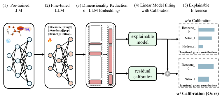
This work proposes a new framework (illustrated in Figure 1), dubbed MoleX, that leverages a linear model augmented with LLM knowledge for explaining complex, non-linear molecular structure-property relationships, motivated by its simplicity and global explainability. To capture these complex relationships, MoleX extracts informative knowledge/embeddings from the LLM, which serve as inputs to fit a linear model. Moreover, we design information bottleneck-inspired fine-tuning and sparsity-inducing dimensionality reduction to maximize task-relevant information in LLM embeddings. Following prior work (Wang et al., 2024), we use Group SELFIES (Cheng et al., 2023)—a text-based molecular representation that partitions molecules into functional groups—as the LLM’s input (as shown in section A.14). Group SELFIES enables LLMs to tokenize molecules into units of functional groups, aligning with chemical concepts at the substructure level. To properly quantify individual functional groups’ contributions to properties, we extract n-gram functional groups from Group SELFIES. These n-grams are fed into the LLM, yielding embeddings where functional groups are semantically distinct and enables a more nuanced analysis of their isolated impacts. Notably, MoleX’s simplicity allows for the approximation of model behaviors over the entire input space during inference, offering global explanations rather than interpreting particular samples.
Despite being augmented with LLM knowledge, linear models still underfit complex, non-linear relationships. Thus, we propose a residual calibration strategy to address prediction errors arising from the gap between high-dimensional LLM embeddings and linear models’ limited expressiveness. Specifically, the residual calibrator is designed to learn the linear model’s residuals. Its outputs are integrated into the linear model, encouraging iterative adjustment of prediction errors. Through sequentially driving residuals toward target values, the residual calibrator recaptures samples missed by the linear model and recovers the original LLM’s predictive power. Consequently, the linear model, incorporated with LLM knowledge and a residual calibrator, provides outstanding predictive performance while enjoying the linear model’s explainability benefit. Our contributions are summarized as
-
1.
We propose MoleX, which extracts LLM knowledge to build a simple yet powerful linear model that identifies chemically meaningful substructures with their interactions for explainable molecular property predictions.
-
2.
We develop optimization-based methods to maximize and preserve task-relevant information in LLM embeddings and theoretically demonstrate their explainability and validity.
-
3.
We design a residual calibration strategy that refits samples missed by the linear model, recovering the LLM’s predictive performance while preserving explainability.
-
4.
We introduce n-gram coefficients, with a theoretical justification, to assess individual functional group contributions to molecular property predictions.
Experiments across 7 datasets demonstrate that MoleX achieves state-of-the-art classification and explanation accuracy while being 300 faster with 100,000 fewer parameters than alternative baselines, highlighting its superiority in predictive performance, explainability, and efficiency.
2 Related Work
Explainable Molecular Property Prediction. Given that molecules can be naturally represented as graphs, a collection of explainable GNNs have been proposed to explain the relationship between molecular structures and properties (Lin et al., 2021; Pope et al., 2019). However, these atom or bond-level explanations are not chemically meaningful to interpret their sophisticated relationships. Besides, through learning chemical semantics, the transformer-based LLMs can effectively capture interactions among substructures (Wang et al., 2024) and thus demonstrated their potential in understanding text-based molecules (Ross et al., 2022; Chithrananda et al., 2020). However, the opaque decision-making process of LLMs obscures their operating principles, risking unfaithful predictions with severe consequences, especially in high-stakes domains like drug discovery (Chen et al., 2024).
Explainability Methods for LLMs. To obtain trustworthy output, various techniques were introduced to unveil the LLM’s explainability. The gradient-based explanations analyze the feature importance by computing output partial derivatives with respect to input (Sundararajan et al., 2017). These methods, nevertheless, lack robustness in their explanations due to sensitivity to data perturbations (Kindermans et al., 2019; Adebayo et al., 2018). The attention-based explanations use attention weights to interpret outputs (Hoover et al., 2020). Yet, recent studies challenge their reliability as attention weights may not consistently reflect true feature importance (Jain & Wallace, 2019; Serrano & Smith, 2019). The perturbation-based explanations elucidate model behaviors by observing output changes in response to input alterations (Ribeiro et al., 2016). However, these explanations are unstable due to the randomness of the perturbations (Agarwal et al., 2021). To resolve these issues, we extract informative embeddings from the LLM to fit a linear model for inference. This approach leverages both the LLM’s knowledge and the linear model’s explainability, offering reliable substructure-level explanations.
3 Preliminaries
Let be a molecular graph, our goal is to train a model to map the molecular representation to its property , denoted as . We first convert the molecular graph into a text-based molecular representation (i.e., Group SELFIES), denoted as , where is the -th functional group and is the dataset we used. The LLM-augmented linear model consists of two modules: an explainable model and a residual calibrator. After the explainable model predicts, its residuals are fed into the residual calibrator , which boosts the performance without incurring any explainability impairment. We denote and as features of explainable model and residual calibrator, as the training loss. To learn and , we freeze parameters of the former and sequentially refit its residuals with the objective:
| (3.1) |
Adapting the approach by Sebastiani (2002), we use n-gram coefficients in the linear model to measure the contributions of decoupled n-gram features/functional groups to molecular properties. Let the n-gram feature takes the coefficient in the linear model, then its contribution score is computed as . This allows us to quantify the contribution of -th functional group to property . Our proof of the validity of using n-gram coefficients as contribution scores is provided in section A.1. In the following parts, we omit the superscript (i) for simplicity.
4 Our Framework: MoleX
MoleX does two things, i.e., () maximizing and preserving the task-relevant information in LLM embeddings via fine-tuning and dimensionality reduction and () extracting these embeddings to build an LLM-augmented linear model with residual calibration. We thus divide it into two stages: LLM knowledge extraction and LLM-augmented linear model fitting. This section details our framework and provides theoretical foundations for its explainability.
4.1 LLM Knowledge Extraction with Improved Informativeness
Fine-tuning. We fine-tune a pre-trained chemical LLM using Group SELFIES data to enhance its understanding of functional group-based molecules. To maximize the linear model’s effectiveness, we aim to extract embeddings that are as informative as possible, fully exploiting the LLM’s interior knowledge. However, empirically fine-tuning the LLM to produce embeddings with the desired informativeness poses a significant challenge. To address this, we apply the Variational Information Bottleneck (VIB) (Alemi et al., 2022) into the fine-tuning process by crafting a training loss to improve embedding informativeness. By optimizing the VIB-based loss function, we encourage the LLM to produce embeddings with the maximum amount of downstream task-relevant information, thus significantly enhancing their informativeness. Particularly, given Group SELFIES inputs , properties , and LLM embeddings , we define as the prior distribution over (e.g., standard normal distribution), and as the variational approximation to the conditional distribution of the properties given the embeddings . The mutual information between and is defined as:
and the mutual information between and is defined as:
Since the marginal distribution is intractable, we approximate it with the prior . Under this approximation, we use as a tractable surrogate for . Inspired by Kingma et al. (2015), we approximate the encoder by a Gaussian distribution. Let and be neural networks that output the mean and covariance matrix of the latent variable . Then, the encoder is given as:
Applying the reparameterization trick, we sample as:
Putting all these together, we design our training loss as:
| (4.1) |
where is the tuning parameter between compression and performance, is the decoder (predictive model), and is the dataset used for fine-tuning. In particular, the first component, , maximizes the task-relevant information about in the produced embeddings . The second component, , minimizes the redundant information from in the produced embeddings . Empirically, we use ChemBERTa-2 (Ahmad et al., 2022) as the foundation LLM for fine-tuning.
In essence, this training loss ensures that the fine-tuned model produces embeddings that capture relevant information about the molecular property while compressing redundant information from . Our design, grounded in the information bottleneck principle, demonstrably leads to informative embeddings with strong explainability. We claim this loss will converge to informative embeddings and provide the proof in section A.2.
Theorem 4.1 (Convergence to an Informative Representation in LLM Fine-tuning).
Let be the loss defined in eq. 4.1. Under the assumptions of the reparameterization trick and the use of stochastic gradient descent, the optimization process converges to a local minimum that yields an informative representation while retaining only the most relevant information from the task.
Embedding Extraction. To capture individual functional group contributions and contextual information, we extract n-grams from Group SELFIES, with selected via cross-validation. To ensure explainability, each n-gram is processed separately by the fine-tuned LLM using a functional group-level tokenizer, encoding a fixed-size embedding vector. These vectors are then aggregated into a single fixed-size embedding that encompasses semantics of all individual n-grams. More precisely, this single embedding contains all chemical semantics at the functional group level and represents the knowledge LLM learned during its training and fine-tuning.
4.2 Dimensionality-reduced embeddings for linear model fitting
Dimensionality Reduction. As the aggregated n-gram embeddings are still high-dimensional and noisy, eliminating the redundancy in these informative embeddings becomes our new problem. Drawing inspiration from Lin et al. (2016), we design an explainable functional principal component analysis (EFPCA) that leads to effective dimensionality reduction. Accordingly, we can preserve a compact yet statistically significant set of features for the linear model. In this part, we demonstrate how to convert this dimensionality reduction into an optimization problem by introducing a sparsity-inducing penalty into the optimization objective function. We define our method as
Definition 4.1 (EFPCA).
Let be a stochastic process defined on a compact interval with mean function . Assume that has a covariance operator derived from the centered data . The EFPCA seeks to find functions that maximize the variance explained by the projections of while promoting sparsity for explainability. Then, the EFPCA solves the following optimization objective:
subject to and ,
where is a tuning parameter that balances the fit and smoothness, measures the length of the support of , promoting sparsity and explainability, and is a tuning parameter controlling the sparsity of .
The penalty term promotes sparsity by encouraging many coefficients to be exactly zero when is sufficiently large. This forces principal components to be exactly zero over extensive portions of the domain . Since is a linear combination of basis functions, zero coefficients directly cause zero contributions from those basis functions across their supports. Specifically, the optimization balances maximizing the variance captured by while minimizing the number of nonzero coefficients, thereby preserving only the most significant components. Furthermore, since the basis functions have local support on subintervals , the nonzero coefficients correspond to basis functions that are active only over those specific intervals. Therefore, the sparsity in the coefficients and the local support of the basis functions result in principal components being nonzero only over certain intervals. Mathematically, the support of is the union of the supports corresponding to the nonzero coefficients . The EFPCA thus produces principal components that are sparse and explainable due to their localized structure, as they highlight the regions where the data exhibits significant variation.
In summary, EFPCA provides a framework for obtaining highly explainable principal components, enabling effective dimensionality reduction. We demonstrate that by combining the sparsity-inducing penalty with the local support of the basis functions, the resulting principal components are both sparse and localized, successfully capturing significant features of the data. In our implementation, we exclude irrelevant functional groups and detect principal ones from the high-dimensional embeddings. Based on this, we claim the following theorem (see our proof in section A.3):
Theorem 4.2.
The EFPCA produces sparse functional principal components that are exactly zero in intervals where the sample curves exhibit minimal variation. Consequently, the FPCs are statistically significant and explanatory, facilitating effective dimensionality reduction.
Linear Model Fitting. Applying dimensionality-reduced n-gram embeddings as features, we train a logistic regression model for our classification tasks, which takes the form:
| (4.2) |
where is the sigmoid function, is the weight vector, is the bias term, and are explainable features as defined in eq. A.11. In our settings, the logistic regression is explainable since the log-odds transformation establishes a linear relationship between features and the target variable such that . Differentiating with respect to a feature component shows that each coefficient quantifies the impact of that feature on the log-odds such that . Moreover, if is a linear transformation, i.e., , the chain rule relates changes in the original features to the log-odds which can be expressed as Therefore, this linearity allows straightforward interpretation of each feature’s influence on the predicted probabilities, making logistic regression highly explainable (Hastie et al., 2009). By directly linking coefficients to features, it offers an intuitive understanding of each feature’s impact on the output.
Residual Calibration. The final step of MoleX involves learning a residual calibrator to improve predictive accuracy while preserving explainability. We freeze parameters of the explainable model and calibrate samples that fails to predict. By optimizing the objective function in eq. A.11, we iteratively fix prediction errors, sequentially driving the overall predictions closer to the target values. The residual calibrator is designed as a linear model, ensuring that the overall model remains explainable. Specifically, we define the residual calibrator with weights corresponding to each residual feature and bias :
Here, represents the residual features obtained from the decomposition of the feature space into orthogonal subspaces such that where contains the explainable features used by , and contains the residual features used by , with the orthogonality condition given by Then, the overall prediction combines the contributions from and :
The orthogonality and linearity between and guarantee that the contributions from and are additive and independent, making the residual calibrator theoretically explainable. Moreover, each feature’s impact on the prediction can be directly understood through the corresponding weights in and . Since and are orthogonal, the inner products and vanish. This ensures that and do not influence each other’s feature contributions, thus preserving the explainability of both models in the combined prediction. We thus formalize the following theorem (see our proof in section A.4):
Theorem 4.3.
Let and be the input and output spaces, respectively. Let be a pre-trained feature mapping, and let be an explainable linear model operating on the explainable features . The residual calibrator , defined on the residual features , captures the variance not explained by in an explainable manner, thereby preserving the overall model’s explainability.
Quantifiable Functional Group Contributions. As described in section 3, we measure the functional group ’s contributions to molecular property using n-gram coefficients. The molecular property distributes its entire semantic information into individual functional groups . Due to the linearity and additivity between and , the scalar coefficient corresponding to in the linear model weighs ’s contributions to in terms of chemical semantics. By taking the dot product of and the embedding of , we obtain a projection length of the functional group in the direction of weight vector, thus quantifying the impact of that functional group on the molecular property. Quantitatively, the larger the absolute value of an n-gram coefficient, the greater the contribution of the corresponding functional group to property. This metric provides a rigorous interpretation of feature contributions, ensuring unbiasedness and significance through OLS estimation (see our proof in section A.1). Using this method, we identify important functional groups from the LLM’s complex embedding space. Furthermore, by incorporating n-gram coefficients and identified functional groups into the molecular graph, we can determine whether identified functional groups bond with each other and infer interactions among them. Essentially, this metric, followed by a mathematical justification, demonstrably provides novel insights into quantifiable functional group contributions in molecular property prediction. Based on this, MoleX reveals chemically meaningful substructures along with their interactions to faithfully explain molecular property predictions.
5 Experiments
5.1 Experimental Settings
Datasets. We empirically evaluate MoleX’s performance on six mutagenicity datasets and one hepatotoxicity dataset. The mutagenicity datasets include Mutag (Debnath et al., 1991), Mutagen (Morris et al., 2020), PTC family (i.e., PTC-FM, PTC-FR, PTC-MM, and PTC-MR) (Toivonen et al., 2003) and the hepatotoxicity dataset includes Liver (Liu et al., 2015). To demonstrate that MoleX can explain molecular properties using chemically meaningful substructures, we introduce the concept of ground truth: substructures verified by domain experts to have significant impacts on molecular properties. The ground truth substructures for six mutagenicity datasets are provided by Lin et al. (2022); Debnath et al. (1991), while those for the hepatotoxicity dataset are provided by Cheng et al. (2023). Further details are available in section A.5.
Evaluation Metrics. We show that MoleX achieves notable predictive performance, explainability performance, and computational efficiency. We apply a specific metric to evaluate each aspect of the model performance. For predictive performance, we define to compute the classification accuracy. For explainability performance, we follow the settings in GNNExplainer (Ying et al., 2019) where explanations are treated as a binary classification of edges (the prediction that matches ground truth substructures as positive, and vice versa) and use the Area Under the Curve (AUC) to quantitatively measure the explanation accuracy. For computational efficiency, we measure the execution time in microseconds for each method.
Baselines. To extensively compare MoleX with different methods, we utilize (1) GNN baselines, including GCN (Kipf & Welling, 2016), DGCNN (Zhang et al., 2018), edGNN (Jaume et al., 2019), GIN (Xu et al., 2018), RW-GNN (Nikolentzos & Vazirgiannis, 2020), DropGNN (Papp et al., 2021), and IEGN (Maron et al., 2018); (2) LLM baselines, including Llama 3.1-8b (Dubey et al., 2024), GPT-4o (Achiam et al., 2023), and ChemBERTa-2 (Ahmad et al., 2022); (3) explainable model baselines, including logistic regression, decision tree (Quinlan, 1986), XGBoost (Chen & Guestrin, 2016), and random forest (Breiman, 2001).
Implementations. Our model is pre-trained on the full ZINC dataset (Irwin et al., 2012) using ChemBERTa-2, with of tokens in each input randomly masked. We then fine-tune this model on the Mutag, Mutagen, PTC-FM, PTC-FR, PTC-MM, PTC-MR, and Liver datasets (in Group SELFIES). To evaluate model performance, we compute the average and standard deviation of each metric for each method after 20 rounds of execution. Further details are provided in section A.6.
5.2 Results
Predictive Performance. Table 1 presents a comparison of predictive performance across different methods. MoleX consistently outperforms all baselines, indicating its robustness and generalizability. Specifically, as a combination of LLMs and explainable models, MoleX achieves better performance compared to either of them (i.e., and higher average classification accuracy than LLM and explainable model baselines, respectively) and demonstrates the effectiveness of augmenting explainable models with LLM knowledge. Moreover, by integrating residual calibration, MoleX raises the average classification accuracy by across seven datasets. Notably, the classification accuracy of our base model, logistic regression, improves by after LLM knowledge augmentation and then by an additional after residual calibration on the Mutag dataset. Therefore, by maximizing task-relevant semantic information in the LLM knowledge and employing a residual calibration strategy, we enable a simple linear model to achieve predictive performance even superior to that of GNNs and LLMs in molecular property predictions.
| Methods | Mutag | Mutagen | PTC-FM | PTC-FR | PTC-MM | PTC-MR | Liver |
|---|---|---|---|---|---|---|---|
| GCN (Kipf & Welling, 2016) | 83.4± 0.4 | 77.2± 0.7 | 56.5± 0.3 | 62.7± 0.5 | 58.3± 0.2 | 52.1± 0.6 | 40.6± 0.3 |
| DGCNN (Zhang et al., 2018) | 86.2± 0.2 | 73.7± 0.5 | 56.1± 0.4 | 64.0± 0.8 | 61.8± 0.7 | 57.1± 0.6 | 45.4± 0.9 |
| edGNN (Jaume et al., 2019) | 85.4± 0.6 | 76.5± 0.3 | 58.7± 0.4 | 66.3± 0.7 | 65.2± 0.6 | 55.1± 0.8 | 43.7± 0.4 |
| GIN (Xu et al., 2018) | 86.1± 0.3 | 81.0± 0.5 | 63.4± 0.8 | 67.8± 0.6 | 66.5± 0.4 | 65.5± 0.4 | 45.2± 0.9 |
| RW-GNN (Nikolentzos & Vazirgiannis, 2020) | 88.2± 0.6 | 79.6± 0.2 | 60.5± 0.7 | 63.2± 0.5 | 61.1± 0.4 | 58.2± 0.6 | 42.9± 0.3 |
| DropGNN (Papp et al., 2021) | 90.3± 0.5 | 82.2± 0.3 | 61.4± 0.8 | 65.3± 0.6 | 62.9± 0.2 | 63.5± 0.7 | 46.1± 0.6 |
| IEGN (Maron et al., 2018) | 83.9± 0.4 | 79.3± 0.5 | 61.9± 0.4 | 60.1± 0.3 | 62.1± 0.4 | 60.7± 0.5 | 44.8± 0.8 |
| LLAMA3.1-8b (Dubey et al., 2024) | 67.6± 3.4 | 50.7± 3.6 | 49.6± 2.6 | 46.2± 3.8 | 42.0± 2.8 | 47.5± 2.8 | 42.2± 2.2 |
| GPT-4o (Achiam et al., 2023) | 73.5± 3.6 | 51.2± 0.5 | 52.7± 2.3 | 53.8± 2.9 | 48.8± 2.4 | 53.7± 1.8 | 44.5± 2.5 |
| ChemBERTa-2 (Ahmad et al., 2022) | 87.3± 2.7 | 77.6± 2.2 | 59.2± 1.9 | 64.8± 2.2 | 59.7± 2.8 | 59.8± 2.4 | 46.3± 2.3 |
| Logistic Regression | 58.3± 1.2 | 55.4± 0.8 | 48.4± 1.1 | 48.3± 1.0 | 48.7± 1.1 | 44.9± 1.0 | 32.5± 0.5 |
| Decision Tree (Quinlan, 1986) | 60.8± 1.7 | 58.6± 1.5 | 43.3± 1.0 | 46.1± 0.7 | 47.2± 0.7 | 43.5± 0.5 | 36.9± 0.8 |
| Random Forest (Breiman, 2001) | 64.6± 1.9 | 60.6± 1.5 | 46.9± 1.2 | 51.4± 1.5 | 51.3± 1.8 | 46.4± 1.1 | 34.8± 1.9 |
| XGBoost (Chen & Guestrin, 2016) | 66.9± 1.2 | 67.6± 1.4 | 51.4± 1.3 | 53.1± 1.4 | 55.8± 1.2 | 49.3± 2.1 | 38.5± 1.8 |
| w/o Calibration | 86.1± 2.2 | 74.4± 1.0 | 59.7± 2.1 | 68.9± 1.9 | 69.3± 2.7 | 61.2± 2.4 | 45.0± 2.0 |
| w/ Calibration (Ours) | 91.6± 2.0 | 83.7± 0.9 | 64.2± 1.4 | 74.4± 1.9 | 76.4± 1.8 | 68.4± 2.3 | 54.9± 2.4 |
Explainability Performance. Table 2 reports the explanation accuracy across different methods. By encoding functional group-level molecular representation, MoleX offers significantly better explainability than baselines on six datasets. Additionally, the residual calibration improves average explanation accuracy by , reflecting a remarkable enhancement of explainability. Similarly, on the Mutag dataset, the explanation accuracy of logistic regression is boosted by a total of via LLM knowledge augmentation and residual calibration. Interestingly, while most methods excel on simpler datasets like Mutag but falter on complex ones like Liver, our method maintains high explanation accuracy across both, showing adaptability and high explanation quality.
| Methods | Mutag | Mutagen | PTC-FM | PTC-FR | PTC-MM | PTC-MR | Liver |
|---|---|---|---|---|---|---|---|
| GCN (Kipf & Welling, 2016) | 81.1± 0.2 | 76.4± 0.2 | 65.3± 0.4 | 67.8± 0.7 | 70.8± 0.8 | 65.1± 0.2 | 62.8± 0.2 |
| DGCNN (Zhang et al., 2018) | 86.3± 1.2 | 87.1± 0.5 | 63.0± 1.3 | 57.0± 1.2 | 63.0± 1.3 | 62.3± 0.8 | 67.5± 1.6 |
| edGNN (Jaume et al., 2019) | 94.7± 0.9 | 74.4± 0.7 | 65.9± 0.5 | 64.1± 0.5 | 66.6± 0.7 | 61.4± 0.7 | 63.2± 0.3 |
| GIN (Xu et al., 2018) | 92.1± 0.2 | 75.6± 0.3 | 67.5± 0.6 | 69.2± 0.5 | 68.5± 0.8 | 61.3± 0.5 | 68.3± 0.9 |
| RW-GNN (Nikolentzos & Vazirgiannis, 2020) | 89.9± 0.6 | 76.7± 0.2 | 65.8± 0.3 | 55.5± 0.3 | 66.9± 0.1 | 59.3± 0.2 | 64.7± 0.5 |
| DropGNN (Papp et al., 2021) | 83.4± 0.2 | 77.4± 0.3 | 68.4± 0.2 | 64.7± 0.4 | 63.2± 0.2 | 57.4± 0.7 | 64.5± 0.8 |
| IEGN (Maron et al., 2018) | 82.0± 0.2 | 77.5± 0.2 | 61.6± 0.6 | 62.6± 0.9 | 69.3± 0.7 | 59.1± 0.7 | 66.6± 0.6 |
| Logistic Regression | 59.2± 0.4 | 50.6± 0.9 | 54.4± 0.3 | 47.7± 0.8 | 49.9± 0.7 | 44.3± 0.7 | 53.8± 0.7 |
| Decision Tree (Quinlan, 1986) | 61.2± 0.2 | 55.7± 1.0 | 56.7± 0.8 | 46.4± 1.1 | 48.1± 0.9 | 39.9± 0.8 | 56.4± 1.0 |
| Random Forest (Breiman, 2001) | 66.7± 1.2 | 57.2± 1.2 | 59.9± 1.7 | 50.9± 1.2 | 55.0± 0.8 | 46.6± 1.1 | 60.7± 1.4 |
| XGBoost (Chen & Guestrin, 2016) | 65.2± 1.2 | 61.3± 1.1 | 58.5± 1.8 | 49.4± 1.8 | 51.6± 1.3 | 50.2± 0.8 | 69.0± 1.4 |
| w/o Calibration | 90.0± 0.9 | 77.7± 1.0 | 68.0± 1.7 | 66.6± 1.1 | 62.0± 1.5 | 67.5± 1.5 | 72.0± 2.0 |
| w/ Calibration (Ours) | 92.6± 1.7 | 89.0± 1.2 | 77.9± 1.5 | 79.3± 1.4 | 72.3± 1.7 | 73.4± 1.3 | 80.3± 1.4 |
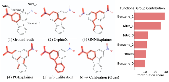
Figure 2 visualizes the explanation for a randomly selected molecule from the Mutag dataset. The ground truth, verified by domain experts, shows that mutagenicity arises from an aromatic functional group (e.g., benzene ring) bonded with another group like nitro or carbonyl. MoleX precisely identifies this ground truth substructure, faithfully explaining molecular structure-property relationships. In contrast, other methods only identify a collection of individual atoms and bonds, failing to recognize chemically meaningful substructures as a whole. For instance, PGExplainer identifies single atoms from multiple benzene rings, whereas atoms alone are insufficient to explain overall molecular properties. Notably, MoleX without calibration identifies two additional elements beyond the ground truth, thus suggesting the significance of residual calibration to explanation accuracy. Moreover, contribution scores elucidate interactions among functional groups, with the benzene-nitro substructure on the upper left receiving a high score, showcasing its importance to mutagenicity as a bonded/interacting entity. More explanation visualizations are in Section A.11.
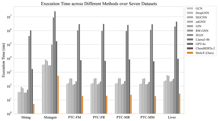
Computational Efficiency. Figure 3 displays the inference time of different methods. Unlike methods that rely on iterative optimization in neural networks, MoleX enables considerably faster inference. Generally, MoleX outperforms both GNNs (at least faster) and LLMs (at least faster) in speed while achieving higher classification and explanation accuracy. MoleX consistently costs the least inference times across all datasets, reinforcing its scalability for real-world applications and large-scale computations on molecular data. In addition to faster inference, MoleX also significantly reduces GPU memory usage compared to baselines by avoiding numerous iterative parameter updates and storage in optimization algorithms. Consequently, the inference power of the linear model is critically augmented by LLM knowledge and residual calibration while preserving the advantage of explainability and computational efficiency.
5.3 Ablation Studies
In this section, we introduce ablation studies on the number of in n-gram, principal components in EFPCA, training iterations of the residual calibrator, and the selection of the base model.
Number of in N-grams. We empirically compare the choice of in n-grams. As shown in fig. 6, the overall model performance improves as increases from 1 to 3, then declines for from 4 to 9. Three of four datasets in our studies indicate the optimal performance at . Increasing captures more contextual semantics, including functional group interactions and raises the model performance. However, overlarge values incorporate excessive or irrelevant contextual information and reduce model utility correspondingly. Further details are in section A.10.
Dimensionality Reduction via EFPCA. We use EFPCA to reduce the dimensionality of LLM embeddings, obtaining explainable and compact embeddings. As shown in fig. 5, cross-validation across four datasets determines the optimal number of principal components. Empirically, components beyond 20 contribute minimally to the molecular property prediction. Additional components yield diminishing returns while increasing model complexity and reducing explainability. Further details are in section A.8. Moreover, we also investigate the effect of our dimensionality reduction. As presented in table 5, we compare the model performance without dimensionality reduction. We find that models using only 20 principal components achieve performance within of models using all components. This means selected components effectively preserve task-relevant information while excluding redundancy. Further details are offered in section A.9.
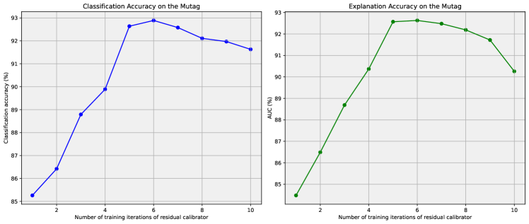
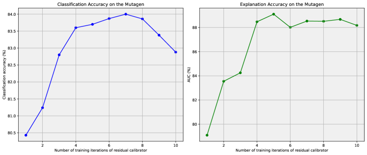
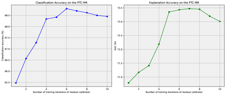
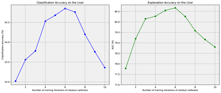
Training Iterations of the Residual Calibrator. We apply the training objective in A.11 to learn a residual calibrator that iteratively refits prediction errors. As shown in fig. 4, we observe that the model performance improves substantially with increasing training iterations until reaching a threshold. Beyond this point, the model overfits the data, leading to a performance decline. This finding suggests the need for an appropriate stopping criterion to balance model performance and prevent overfitting. Empirically, the optimal number of training iterations is 5. Further details and a theoretical demonstration are offered in section A.7.
Selection of the Base Model. Aside from the logistic regression, we examine the effect of LLM augmentation using other statistical learning models as the base model. The classification and explanation accuracy are reported in table 6 and table 7, respectively. All statistical learning models augmented with LLM knowledge and residual calibration outperform GNNs and LLMs. Besides, more complicated models, like XGBoost and random forest, achieve better performance in both classification and explanation accuracy than simple models like LASSO. Therefore, LLM knowledge is capable of augmenting a model on top of its original predictive capabilities, evidencing the effectiveness and generalizability of our method. However, model complexity generally trades off with explainability. Considering this, we select the logistic regression as our base model for its optimal balance between explainability and performance. Further details are offered in section A.12.
6 Conclusion
This work develops MoleX, a novel framework utilizing LLM knowledge to build a powerful linear model for accurate molecular property predictions with chemically meaningful explanations. Specifically, MoleX extracts task-relevant knowledge from LLM embeddings using information bottleneck-inspired fine-tuning and sparsity-inducing dimensionality reduction to train a linear model for explainable inference. Additionally, a residual calibration module is designed to recover the original LLM’s performance and further enhance the linear model via recapturing prediction errors. During its inference, MoleX precisely reveals crucial substructures with their interactions as explanations. Notably, MoleX enjoys the advantage of LLM’s predictive power while preserving the linear model’s intrinsic explainability. Extensive theoretical and empirical analysis demonstrate MoleX’s exceptional predictive performance, explainability, and efficiency.
References
- Achiam et al. (2023) Josh Achiam, Steven Adler, Sandhini Agarwal, Lama Ahmad, Ilge Akkaya, Florencia Leoni Aleman, Diogo Almeida, Janko Altenschmidt, Sam Altman, Shyamal Anadkat, et al. Gpt-4 technical report. arXiv preprint arXiv:2303.08774, 2023.
- Adebayo et al. (2018) Julius Adebayo, Justin Gilmer, Michael Muelly, Ian Goodfellow, Moritz Hardt, and Been Kim. Sanity checks for saliency maps. Advances in neural information processing systems, 31, 2018.
- Agarwal et al. (2021) Sushant Agarwal, Shahin Jabbari, Chirag Agarwal, Sohini Upadhyay, Steven Wu, and Himabindu Lakkaraju. Towards the unification and robustness of perturbation and gradient based explanations. In International Conference on Machine Learning, pp. 110–119. PMLR, 2021.
- Ahmad et al. (2022) Walid Ahmad, Elana Simon, Seyone Chithrananda, Gabriel Grand, and Bharath Ramsundar. Chemberta-2: Towards chemical foundation models. arXiv preprint arXiv:2209.01712, 2022.
- Alemi et al. (2022) Alexander A Alemi, Ian Fischer, Joshua V Dillon, and Kevin Murphy. Deep variational information bottleneck. In International Conference on Learning Representations, 2022.
- Breiman (2001) Leo Breiman. Random forests. Machine learning, 45:5–32, 2001.
- Chen et al. (2024) Jialin Chen, Shirley Wu, Abhijit Gupta, and Rex Ying. D4explainer: In-distribution explanations of graph neural network via discrete denoising diffusion. Advances in Neural Information Processing Systems, 36, 2024.
- Chen & Guestrin (2016) Tianqi Chen and Carlos Guestrin. Xgboost: A scalable tree boosting system. In Proceedings of the 22nd acm sigkdd international conference on knowledge discovery and data mining, pp. 785–794, 2016.
- Cheng et al. (2023) Austin H Cheng, Andy Cai, Santiago Miret, Gustavo Malkomes, Mariano Phielipp, and Alán Aspuru-Guzik. Group selfies: a robust fragment-based molecular string representation. Digital Discovery, 2(3):748–758, 2023.
- Chithrananda et al. (2020) Seyone Chithrananda, Gabriel Grand, and Bharath Ramsundar. Chemberta: Large-scale self-supervised pretraining for molecular property prediction. arXiv preprint arXiv:2010.09885, 2020.
- Debnath et al. (1991) Asim Kumar Debnath, Rosa L Lopez de Compadre, Gargi Debnath, Alan J Shusterman, and Corwin Hansch. Structure-activity relationship of mutagenic aromatic and heteroaromatic nitro compounds. correlation with molecular orbital energies and hydrophobicity. Journal of medicinal chemistry, 34(2):786–797, 1991.
- Dubey et al. (2024) Abhimanyu Dubey, Abhinav Jauhri, Abhinav Pandey, Abhishek Kadian, Ahmad Al-Dahle, Aiesha Letman, Akhil Mathur, Alan Schelten, Amy Yang, Angela Fan, et al. The llama 3 herd of models. arXiv preprint arXiv:2407.21783, 2024.
- Hastie et al. (2009) Trevor Hastie, Robert Tibshirani, Jerome H Friedman, and Jerome H Friedman. The elements of statistical learning: data mining, inference, and prediction, volume 2. Springer, 2009.
- Hoover et al. (2020) Benjamin Hoover, Hendrik Strobelt, and Sebastian Gehrmann. exbert: A visual analysis tool to explore learned representations in transformer models. In Proceedings of the 58th Annual Meeting of the Association for Computational Linguistics: System Demonstrations, pp. 187–196, 2020.
- Irwin et al. (2012) John J Irwin, Teague Sterling, Michael M Mysinger, Erin S Bolstad, and Ryan G Coleman. Zinc: a free tool to discover chemistry for biology. Journal of chemical information and modeling, 52(7):1757–1768, 2012.
- Jain & Wallace (2019) Sarthak Jain and Byron C Wallace. Attention is not explanation. In Proceedings of the 2019 Conference of the North American Chapter of the Association for Computational Linguistics: Human Language Technologies, Volume 1 (Long and Short Papers), pp. 3543–3556, 2019.
- Jaume et al. (2019) Guillaume Jaume, An-Phi Nguyen, Maria Rodriguez Martinez, Jean-Philippe Thiran, and Maria Gabrani. edgnn: A simple and powerful gnn for directed labeled graphs. In International Conference on Learning Representations, 2019.
- Kindermans et al. (2019) Pieter-Jan Kindermans, Sara Hooker, Julius Adebayo, Maximilian Alber, Kristof T Schütt, Sven Dähne, Dumitru Erhan, and Been Kim. The (un) reliability of saliency methods. Explainable AI: Interpreting, explaining and visualizing deep learning, pp. 267–280, 2019.
- Kingma et al. (2015) Durk P Kingma, Tim Salimans, and Max Welling. Variational dropout and the local reparameterization trick. Advances in neural information processing systems, 28, 2015.
- Kipf & Welling (2016) Thomas N Kipf and Max Welling. Semi-supervised classification with graph convolutional networks. In International Conference on Learning Representations, 2016.
- Lin et al. (2021) Wanyu Lin, Hao Lan, and Baochun Li. Generative causal explanations for graph neural networks. In International Conference on Machine Learning, pp. 6666–6679. PMLR, 2021.
- Lin et al. (2022) Wanyu Lin, Hao Lan, Hao Wang, and Baochun Li. Orphicx: A causality-inspired latent variable model for interpreting graph neural networks. In Proceedings of the IEEE/CVF Conference on Computer Vision and Pattern Recognition, pp. 13729–13738, 2022.
- Lin et al. (2016) Zhenhua Lin, Liangliang Wang, and Jiguo Cao. Interpretable functional principal component analysis. Biometrics, 72(3):846–854, 2016.
- Liu et al. (2015) Ruifeng Liu, Xueping Yu, and Anders Wallqvist. Data-driven identification of structural alerts for mitigating the risk of drug-induced human liver injuries. Journal of cheminformatics, 7:1–8, 2015.
- Liu et al. (2022) Yibing Liu, Haoliang Li, Yangyang Guo, Chenqi Kong, Jing Li, and Shiqi Wang. Rethinking attention-model explainability through faithfulness violation test. In International Conference on Machine Learning, pp. 13807–13824. PMLR, 2022.
- Luo et al. (2020) Dongsheng Luo, Wei Cheng, Dongkuan Xu, Wenchao Yu, Bo Zong, Haifeng Chen, and Xiang Zhang. Parameterized explainer for graph neural network. Advances in neural information processing systems, 33:19620–19631, 2020.
- Maron et al. (2018) Haggai Maron, Heli Ben-Hamu, Nadav Shamir, and Yaron Lipman. Invariant and equivariant graph networks. In International Conference on Learning Representations, 2018.
- Mirghaffari et al. (2021) Nourollah Mirghaffari, Riccardo Iannarelli, Christian Ludwig, and Michel J Rossi. Coexistence of reactive functional groups at the interface of a powdered activated amorphous carbon: a molecular view. Molecular Physics, 119(17-18):e1966110, 2021.
- Morris et al. (2020) Christopher Morris, Nils M Kriege, Franka Bause, Kristian Kersting, Petra Mutzel, and Marion Neumann. Tudataset: A collection of benchmark datasets for learning with graphs. arXiv preprint arXiv:2007.08663, 2020.
- Nikolentzos & Vazirgiannis (2020) Giannis Nikolentzos and Michalis Vazirgiannis. Random walk graph neural networks. Advances in Neural Information Processing Systems, 33:16211–16222, 2020.
- Papp et al. (2021) Pál András Papp, Karolis Martinkus, Lukas Faber, and Roger Wattenhofer. Dropgnn: Random dropouts increase the expressiveness of graph neural networks. Advances in Neural Information Processing Systems, 34:21997–22009, 2021.
- Pope et al. (2019) Phillip E Pope, Soheil Kolouri, Mohammad Rostami, Charles E Martin, and Heiko Hoffmann. Explainability methods for graph convolutional neural networks. In Proceedings of the IEEE/CVF conference on computer vision and pattern recognition, pp. 10772–10781, 2019.
- Proietti et al. (2024) Michela Proietti, Alessio Ragno, Biagio La Rosa, Rino Ragno, and Roberto Capobianco. Explainable ai in drug discovery: self-interpretable graph neural network for molecular property prediction using concept whitening. Machine Learning, 113(4):2013–2044, 2024.
- Quinlan (1986) J. Ross Quinlan. Induction of decision trees. Machine learning, 1:81–106, 1986.
- Ribeiro et al. (2016) Marco Tulio Ribeiro, Sameer Singh, and Carlos Guestrin. ” why should i trust you?” explaining the predictions of any classifier. In Proceedings of the 22nd ACM SIGKDD international conference on knowledge discovery and data mining, pp. 1135–1144, 2016.
- Ross et al. (2022) Jerret Ross, Brian Belgodere, Vijil Chenthamarakshan, Inkit Padhi, Youssef Mroueh, and Payel Das. Large-scale chemical language representations capture molecular structure and properties. Nature Machine Intelligence, 4(12):1256–1264, 2022.
- Sebastiani (2002) Fabrizio Sebastiani. Machine learning in automated text categorization. ACM computing surveys (CSUR), 34(1):1–47, 2002.
- Serrano & Smith (2019) Sofia Serrano and Noah A Smith. Is attention interpretable? In Proceedings of the 57th Annual Meeting of the Association for Computational Linguistics, pp. 2931–2951, 2019.
- Sundararajan et al. (2017) Mukund Sundararajan, Ankur Taly, and Qiqi Yan. Axiomatic attribution for deep networks. In International conference on machine learning, pp. 3319–3328. PMLR, 2017.
- Toivonen et al. (2003) Hannu Toivonen, Ashwin Srinivasan, Ross D King, Stefan Kramer, and Christoph Helma. Statistical evaluation of the predictive toxicology challenge 2000–2001. Bioinformatics, 19(10):1183–1193, 2003.
- Voita et al. (2019) Elena Voita, David Talbot, Fedor Moiseev, Rico Sennrich, and Ivan Titov. Analyzing multi-head self-attention: Specialized heads do the heavy lifting, the rest can be pruned. In Proceedings of the 57th Annual Meeting of the Association for Computational Linguistics, pp. 5797–5808, 2019.
- Wang et al. (2024) Zhenzhong Wang, Zehui Lin, Wanyu Lin, Ming Yang, Minggang Zeng, and Kay Chen Tan. Explainable Molecular Property Prediction: Aligning Chemical Concepts with Predictions via Language Models. arXiv preprint arXiv:2405.16041, 2024.
- Weininger (1988) David Weininger. Smiles, a chemical language and information system. 1. introduction to methodology and encoding rules. Journal of chemical information and computer sciences, 28(1):31–36, 1988.
- Wu et al. (2023a) Zhenxing Wu, Jihong Chen, Yitong Li, Yafeng Deng, Haitao Zhao, Chang-Yu Hsieh, and Tingjun Hou. From black boxes to actionable insights: a perspective on explainable artificial intelligence for scientific discovery. Journal of Chemical Information and Modeling, 63(24):7617–7627, 2023a.
- Wu et al. (2023b) Zhenxing Wu, Jike Wang, Hongyan Du, Dejun Jiang, Yu Kang, Dan Li, Peichen Pan, Yafeng Deng, Dongsheng Cao, Chang-Yu Hsieh, et al. Chemistry-intuitive explanation of graph neural networks for molecular property prediction with substructure masking. Nature Communications, 14(1):2585, 2023b.
- Xia et al. (2024) Jun Xia, Lecheng Zhang, Xiao Zhu, Yue Liu, Zhangyang Gao, Bozhen Hu, Cheng Tan, Jiangbin Zheng, Siyuan Li, and Stan Z Li. Understanding the limitations of deep models for molecular property prediction: Insights and solutions. Advances in Neural Information Processing Systems, 36, 2024.
- Xiang et al. (2023) Yan Xiang, Yu-Hang Tang, Guang Lin, and Daniel Reker. Interpretable molecular property predictions using marginalized graph kernels. Journal of Chemical Information and Modeling, 63(15):4633–4640, 2023.
- Xu et al. (2018) Keyulu Xu, Weihua Hu, Jure Leskovec, and Stefanie Jegelka. How powerful are graph neural networks? In International Conference on Learning Representations, 2018.
- Yang et al. (2019) Kevin Yang, Kyle Swanson, Wengong Jin, Connor Coley, Philipp Eiden, Hua Gao, Angel Guzman-Perez, Timothy Hopper, Brian Kelley, Miriam Mathea, et al. Analyzing learned molecular representations for property prediction. Journal of chemical information and modeling, 59(8):3370–3388, 2019.
- Ying et al. (2019) Zhitao Ying, Dylan Bourgeois, Jiaxuan You, Marinka Zitnik, and Jure Leskovec. Gnnexplainer: Generating explanations for graph neural networks. Advances in neural information processing systems, 32, 2019.
- Zhang et al. (2018) Muhan Zhang, Zhicheng Cui, Marion Neumann, and Yixin Chen. An end-to-end deep learning architecture for graph classification. In Proceedings of the AAAI conference on artificial intelligence, volume 32, 2018.
Appendix A Appendix
A.1 Proof of N-Gram Coefficients as Valid Contribution Scores for Decoupled n-gram Features
In this section, we demonstrate that n-gram coefficients in the linear model can be interpreted as feature contribution scores based on the statistical properties of the linear model.
Proof.
Suppose is the matrix of n-gram embeddings, where each row is the embedding of the -th n-gram. Let be the embedding of the -th feature in the -th n-gram, and suppose that each n-gram consists of features ( is a constant across all n-grams). Let denote the contribution score of the -th feature in the -th n-gram. We formulate the following assumptions based on OLS properties to ensure the validity of using n-gram coefficients as contribution scores:
-
1.
Linearity. The relationship between the input embeddings and the output is linear. Namely, for all ,
where is the true coefficient vector, and is the error term.
-
2.
N-gram Embedding Decomposition. Each n-gram embedding is the average of its constituent feature embeddings:
-
3.
Ordinary Least Squares (OLS). The linear model is estimated using OLS by minimizing the residual sum of squares:
-
4.
Error Properties.
-
(a)
Zero Mean Errors. The errors have zero mean given the embeddings:
-
(b)
Homoscedasticity. The errors have constant variance given the embeddings:
where is a positive constant.
-
(c)
No Autocorrelation. The errors are uncorrelated with each other:
-
(a)
-
5.
Full Rank. The matrix is invertible (i.e., has full column rank).
We define the contribution score of each decoupled n-gram feature as follows:
Definition A.1.
The feature contribution score for the -th feature in the -th n-gram is defined as
where is the estimated coefficient vector from the linear model.
Lemma A.1 (Prediction as Sum of Feature Contributions).
Under Assumption 2, the predicted output for the -th n-gram is
Proof.
Using the embedding decomposition and the definition of the contribution scores, we have
This completes the proof. ∎
Theorem A.2 (Contribution Scores Quantify Individual Feature Contributions).
Under the Linearity assumption (Assumption 1), the feature contribution scores quantify the contributions of individual features to the prediction .
Proof.
From Lemma A.1, the predicted value is given as the average of the feature contribution scores . Specifically,
This equation shows that each feature’s contribution score directly influences the prediction . Therefore, quantifies the contribution of the -th feature in the -th n-gram to the prediction.
This completes the proof. ∎
Due to the statistical properties of the OLS estimator, we formulate the following theorem:
Theorem A.3 (Properties of the OLS Estimator).
Proof.
We prove each property as follows.
(1) Unbiasedness: The OLS estimator is given by
Substituting , we have
Taking expectations conditional on and using Assumption 4(a),
(3) Consistency: As , under the Law of Large Numbers,
where is positive definite due to Assumption 5. Additionally,
since has zero mean and finite variance. Therefore,
This completes the proof. ∎
To validate the convergence of the contribution scores, we introduce the asymptotic normality of the OLS estimator.
Corollary A.1 (Asymptotic Normality).
If the error terms are independently and identically normally distributed with mean zero and variance , then we have
where .
Proof.
Under the given conditions, the Central Limit Theorem applies to the sum . Specifically,
As , and . Therefore,
This completes the proof. ∎
Lemma A.4 (Variance of ).
The variance of the estimated feature contribution score is
Proof.
Since is a linear function of , its variance conditional on is
using the result from Theorem A.3(2).
This completes the proof. ∎
Finally, we demonstrate the statistical significance of the feature contribution scores based on the n-gram coefficients.
Theorem A.5 (t-Statistic for Feature Contribution Scores).
Under the above assumptions, the t-statistic for testing is given as
Proof.
The standard error of is
Therefore, the t-statistic is
Under the null hypothesis and the assumption of normality, follows a t-distribution with degrees of freedom.
This completes the proof. ∎
From Theorem A.2, we have shown that the feature contribution scores represent the contributions of individual features to the predictions . The statistical properties outlined in Theorem A.3 and Lemma A.4 guarantee that these estimates are reliable and their statistical significance can be assessed.
Therefore, we prove that each feature’s contribution to the prediction can be quantified by its corresponding coefficient in the linear model, enable us to assess the importance of individual features. By mathematically linking the model coefficients to the feature contributions, we validate the use of these coefficients as measures of feature importance. We also conclude that using n-gram coefficients derived from feature embeddings and model coefficients as contribution scores for input features is valid and grounded in the statistical properties of the linear model. The n-gram coefficients used in our implementation faithfully reflect the importance and contribution of each input feature in our linear model. By expressing the predicted output as the sum of individual feature contributions, we effectively decouple the influence of each feature/functional group on the output/molecular property. This decoupling allows us to isolate the effect of each n-gram feature or functional group on the molecular property . Consequently, the contribution scores provide a quantitative measure of how each functional group impacts the molecular property.
This completes the proof. ∎
A.2 Proof of theorem 4.1 (Explainability of VIB-based Training Objectives)
Proof.
We demonstrate the Variational Information Bottleneck (VIB) framework, which aims to learn a compressed representation of input variable that preserves maximal information about the target variable while being minimally informative about itself. This is achieved by optimizing the objective function as follows:
where is mutual information, is a tuning parameter, and is the parameters of the encoder. Our goal is to derive a tractable variational lower bound of this objective function that can be optimized using stochastic gradient descent.
Definition A.2 (Mutual Information).
For random variables and with joint distribution , the mutual information is defined as
Alternatively, it can be expressed as
Definition A.3 (Kullback-Leibler Divergence).
For probability distributions and over the same probability space, the KL divergence from to is defined as
Definition A.4 (Conditional Entropy).
The conditional entropy is defined as
We then formulate the problem. Let be a dataset of input-output pairs sampled from an unknown distribution . The encoder parameterizes the conditional distribution of given , and the decoder parameterizes the conditional distribution of given . Our objective is to optimize the parameters and by maximizing the Information Bottleneck Lagrangian as follows:
However, direct computation of and is intractable. Therefore, we derive variational bounds to make the optimization objective tractable. We start by applying the lemma as
Lemma A.6 (Variational Upper Bound on ).
The mutual information can be upper-bounded as
where is an arbitrary prior distribution over .
Proof.
We start by rewriting as
Since , and is intractable, we introduce an approximate prior and apply the following decomposition:
Thus, we have:
Since , it follows that:
This completes the proof. ∎
Lemma A.7 (Variational Lower Bound on ).
The mutual information can be lower-bounded as
Proof.
By the definition of mutual information:
Since is intractable, we introduce a variational approximation to get:
Using Jensen’s inequality and the non-negativity of KL divergence, we have:
Neglecting the KL divergence term (assuming approximates well), we have:
Thus:
This completes the proof. ∎
Now we can formulate the Variational Information Bottleneck (VIB) Objective. Particularly, combining Lemmas lemma A.6 and lemma A.7, we obtain a tractable objective function.
Proposition A.8 (Variational Lower Bound on the Information Bottleneck Objective).
The Information Bottleneck Lagrangian can be lower-bounded by the variational objective function:
Proof.
Starting from the original objective:
Applying the upper bound of from Lemma lemma A.6 and the lower bound of from Lemma lemma A.7, we get:
Since is constant with respect to and , we can ignore it for optimization purposes. We define the variational objective function as
which serves as an upper bound on . Minimizing will therefore minimize , satisfying our optimization goal.
This completes the proof. ∎
In our fine-tuning stage, since the expectation of is approximated by empirical samples from the dataset , and the expectations of are approximated by Monte Carlo sampling with reparameterization trick. Thus, the loss function is expressed as (note that this is a generalized form of our designed loss function shown in eq. 4.1):
To demonstrate the convergence, we have:
Theorem A.9 (Convergence of Stochastic Gradient Descent).
Under standard assumptions of stochastic optimization (bounded gradients, appropriate learning rates, etc.), stochastic gradient descent (SGD) converges to a local minimum of .
Proof.
While the neural network training is non-convex, empirical and theoretical results in optimization, SGD can converge to critical points (which may be local minima, maxima, or saddle points) provided the loss function is smooth (i.e., continuously differentiable) and the gradients are Lipschitz continuous.
Given that is composed of differentiable functions, and the gradients with respect to and can be computed via back-propagation, the convergence to a local minimum is attainable under proper value of learning rate and optimization parameters.
This completes the proof. ∎
We express the corollary of our learned molecular representation after fine-tuning as
Corollary A.2 (Informative and Compressed Molecular Representation).
At convergence, the learned representation satisfies:
Proof.
By optimizing the variational objective function , we are effectively minimizing an upper bound on (Lemma lemma A.6) and maximizing a lower bound on (Lemma lemma A.7). The trade-off between the two objectives is controlled by .
As increases, more emphasis is placed on minimizing , leading to a more compressed representation that preserves only the most task-relevant information about .
This completes the proof. ∎
Specifically, as the first term in the loss function encourages the embeddings to be highly predictive of , it intrinsically captures the task-relevant information. Meanwhile, the second term penalizes the complexity of by forcing it to be close to the prior , thereby excluding unnecessary information from . These objectives ensure that the embeddings are both task-relevant and compact, containing minimal spurious data. Additionally, through the derivation of variational bounds and the construction of a tractable objective function, we have shown that minimizing allows us to learn a molecular representation that captures maximal information about while being minimally informative about , in accordance with the Information Bottleneck principle. The optimization of via SGD converges to a local minimum under standard optimization assumptions. Therefore, we learn an informative embedding after fine-tuning the pre-trained LLM, and we thus can extract the embedding with improved informativeness.
In conclusion, by framing the fine-tuning within the VIB framework, we derive this approach that balances the essential information for property prediction with the elimination of irrelevant details from the input molecular representation . This theoretical foundation ensures that MoleX effectively focuses on extracting the most relevant features needed for accurate predictions.
This completes the proof. ∎
A.3 Proof of theorem 4.2 (Explainability of EFPCA)
Proof.
To demonstrate the explainability of the EFPCA, we will showcase how the incorporation of a sparsity-inducing penalty and the use of basis functions with local support lead to explainable FPCs.
We first formulated the EFPCA as an optimization problem. The EFPCA seeks to find FPCs by solving the following optimization
| (A.1) |
subject to
| (A.2) |
and
| (A.3) |
where
-
•
is the empirical covariance operator of the centered stochastic process .
-
•
is the standard inner product.
-
•
is the squared norm.
-
•
denotes the second derivative of .
-
•
penalizes the roughness of .
-
•
is a smoothing parameter balancing the trade-off between variance explanation and smoothness.
-
•
is the roughness-penalized inner product.
-
•
measures the support length of .
-
•
is a tuning parameter controlling the sparsity of .
We then construct the expansion in basis functions with local Support. In particularly, we choose a set of basis functions that have local support on the interval , such as B-spline basis functions. Each is nonzero only over a subinterval . We expand in terms of these basis functions:
| (A.4) |
where is the coefficient vector for the -th principal component. Therefore, the reformulation of the optimization problem in terms of coefficients can be expressed. We substitute the expansion (A.4) into the optimization problem(A.1), and express the objective function and constraints in terms of :
| (A.5) |
subject to
| (A.6) |
and
| (A.7) |
where is the matrix with entries , is the roughness-penalized Gram matrix with entries , counts the number of nonzero coefficients in , and are the coefficient vectors of previously computed principal components.
Through the introduction of sparsity-inducing penalty, we can observe that the term in the objective function (A.5) is a sparsity-inducing penalty that encourages many coefficients to be exactly zero. When is sufficiently large, the optimization process favors solutions where is minimized, effectively shrinking less significant coefficients to zero.
Furthermore, define the index set of nonzero coefficients:
| (A.8) |
The principal component can then be expressed as:
| (A.9) |
Since each has support only on , the support of is:
| (A.10) |
This means is exactly zero outside the union of the supports of the basis functions corresponding to nonzero coefficients. The localization of to specific intervals directly indicates regions where the functional data exhibits significant variation. The sparsity in the coefficients leads to sparsity in , making the principal components explainable:
-
•
Identification of Significant Intervals. The nonzero coefficients correspond to basis functions whose supports cover intervals where the data carries significant information.
-
•
Reduction of Complexity. By focusing on a subset of intervals, simplifies the understanding of functional variability.
-
•
Improved Explainability. We can easily interpret by examining the intervals where it is nonzero, relating these regions back to the original context of the data.
Besides, we introduce the roughness penalty for smoothness. The roughness penalty in the normalization constraint (A.2) and the inner product ensures that remains smooth within its support. This avoids overfitting and maintains the functional integrity of the PCs.
In conclusion, by incorporating a sparsity-inducing penalty and utilizing basis functions with local support, the EFPCA produces FPCs that are both sparse and localized. This leads to principal components that are nonzero only over intervals where the data contains significant variation, making them intrinsically explainable. By effectively encouraging sparsity, the EFPCA filters out task-irrelevant information in the high-dimensional LLM embeddings, preserving only the most informative features associated with the task. Consequently, the dimensionality reduction achieved is efficient and designed to exclude noisy and redundant information in the embeddings. Therefore, the EFPCA achieves explainability through its optimization framework that deliver sparsity, assisting dimensionality reduction while providing insights into the underlying functional data. The EFPCA can effectively reduce the dimensionality of the extracted LLM embeddings as the solution of the objective function can be optimized to become sparser. In our implementation, the statistically significant features are kept in an explainable manner.
This completes the proof. ∎
A.4 Proof of theorem 4.3 (Explainability of Residual Calibration)
Proof.
We demonstrate that the residual calibrator is explainable when combined with the explainable linear model , under certain conditions.
Let be the input space, and be the output space. Let be a feature extraction function mapping inputs to a Hilbert space of dimension , equipped with inner product and norm . Assume that can be decomposed into two orthogonal components via the direct sum decomposition of :
where and are closed linear subspaces of , satisfying the following conditions:
Then, for each , we have:
where is the projection of onto , and is the projection onto . The projections are given by the orthogonal projection operators and , such that:
where is the identity operator on . Let be an explainable model, assumed to be linear:
where is the weight vector, and is the bias term. Similarly, let be the residual calibrator, also linear:
where and . Then the combined model’s prediction is:
Define and , so that we have:
Since , , and , it follows that:
To demonstrate the explainability of , we consider the following statistical perspectives to verify its explainability (Hastie et al., 2009):
Linearity. Since is linear and operates on , its influence on the prediction is straightforward. Each component contributes to proportionally to , which is:
This allows us to quantify the effect of each residual feature on the prediction.
Orthogonality. The orthogonality of and ensures that the contributions from and are independent. Specifically, the covariance between and is zero:
where and , assuming and have finite second moments.
Variance Decomposition. The total variance of the prediction can be decomposed as
due to the independence of and . This decomposition assists in understanding how much variability each component contributes.
Optimization Decoupling. Consider the expected loss over the data distribution :
where is a convex loss function, such as squared loss .
Due to the orthogonality, the gradients with respect to and are:
where denotes the derivative of with respect to its first argument. Since and are orthogonal and belong to different subspaces, the optimization of and can be treated separately, or decoupled. Specifically, we can minimize by independently minimizing:
Preservation of Explainability. The explainability of is preserved because operates on features orthogonal to those used by , and their contributions to are additive:
Each term can be examined independently. The explainable component aligns with the original explainable model, while the residual component adds adjustments based on the residual features.
Feature Contributions Interpretation. For any given feature , its contribution to the prediction can be determined based on whether it belongs to or . Specifically:
This allows for a granular interpretation of the impact of each feature on the prediction.
Mathematical Justification. From a functional analysis perspective, since both and are bounded linear operators on and , respectively, and these subspaces are closed in , their sum is a bounded linear operator on . The boundedness ensures stability and well-posedness of the model. Moreover, the spectral properties of the operators can be analyzed separately. For example, if we consider the operator norms:
These norms provide insight into the maximum amplification of inputs by the respective operators.
The orthogonality and linearity between and ensure that the contributions from and are additive and independent, making the residual calibrator explainable when combined with . Each feature’s impact on the prediction can be directly understood through the corresponding weights and , enabling straightforward model interpretation. Specifically, since and are orthogonal, the cross terms and vanish, so and do not influence each other’s feature contributions.
Therefore, under the conditions of linearity and orthogonality, the residual calibrator preserves explainability when combined with . The linearity ensures transparency in how input features affect the output, as each feature’s contribution is directly proportional to its weight. The orthogonality guarantees that the explainability of is not compromised by since they operate on separate feature spaces. In our implementation, these conditions are satisfied by utilizing logistic regression models for both and , making our method provably explainable.
This completes the proof. ∎
A.5 Dataset Details
We use six mutagenicity datasets and one hepatotoxicity dataset. The mutagenicity datasets are: Mutag (Debnath et al., 1991), Mutagen (Morris et al., 2020), PTC-FM (Toivonen et al., 2003), PTC-FR (Toivonen et al., 2003), PTC-MM (Toivonen et al., 2003), PTC-MR (Toivonen et al., 2003), and the hepatotoxicity dataset is the Liver (Liu et al., 2015). Followed by Morris et al. (2020), we list the summary statistics of these datasets as
| Dataset | Mutag | Mutagen | PTC-FM | PTC-FR | PTC-MM | PTC-MR | Liver |
|---|---|---|---|---|---|---|---|
| Samples | 188 | 4337 | 349 | 351 | 336 | 344 | 587 |
| Classes | 2 | 2 | 2 | 2 | 2 | 2 | 3 |
| Ground truth | 120 | 724 | 58 | 49 | 51 | 61 | 187 |
The ground truth indicates the true molecular substructures that impact molecular properties. As verified by Lin et al. (2022); Debnath et al. (1991), the ground truth substructures for six mutagenicity datasets consist of an aromatic group, such as a benzene ring, bonded with another functional group, such as methoxy, oxhydryl, nitro, or carboxyl groups (note that ground truth exists only for the mutagenic class). For the Liver dataset, the ground truth substructures annotated by chemists are: fused tricyclic saturated hydrocarbon moiety, hydrazines, arylacetic acid, sulfonamide moiety, aniline moiety, a class of proton pump inhibitor drugs, acyclic bivalent sulfur moiety, acyclic di-aryl ketone moiety, para oxygen and nitrogen di-substituted benzene ring, a relatively small number of com- pounds in the expanded LiverTox dataset, halogen atom bonded to a carbon, and fused tricyclic structural moiety. A detailed illustration of Liver’s ground truth substructures are provided by Liu et al. (2015).
A.6 Implementation Details
Our model is pre-trained on all data in the ZINC dataset (over million compounds) using ChemBERTa-2, with (default setting) of tokens in each input randomly masked. We extract all functional groups in the ZINC dataset as the vocabulary to expand the LLM’s tokenizer so that the fine-tuned LLM can better encode functional group-level inputs. We then fine-tune this model on Mutag, Mutagen, PTC-FM, PTC-FR, PTC-MM, PTC-MR, and Liver datasets. The fine-tuning is conducted on 1 NVIDIA RTX3090 GPU for about 3 hours. The detailed hyperparameters with their values are given in table 4. For experiments on model performance, we employ chain-of-thought prompting for the molecular property prediction tasks on LLMs.
| Hyperparameter | Value |
|---|---|
| learning rate | 1e-5 |
| batch size | 128 |
| epochs | 30 |
| weight decay | 0.01 |
| gradient clipping | 1.0 |
| warmup proportion | 0.06 |
| max sequence length | 1024 |
| optimizer | AdamW |
| dropout rate | 0.1 |
| gradient accumulation steps | 1 |
| mixed precision training | True |
A.7 Does the Residual Calibrator Improves Model Performance by training with more iterations?
We employ the training objective in A.11 to learn a residual calibrator that iteratively recaptures samples the linear model fails to predict accurately. We empirically study how training iterations influence the overall model predictions. As shown in fig. 4, we visualize the model performance on the Mutag, Mutagen, PTC-MR, and Liver datasets under different numbers of training iterations. As training iterations increase, model performance improves significantly until reaching a threshold. This suggests that more iterations on our designed loss lead to better performance. After the threshold, the model overfits the data, resulting in performance degradation. Therefore, increasing the number of training iterations helps improve model performance. Empirically, we found that 5 iterations yield optimal performance. A theoretical demonstration shows that training with multiple iterations increases model performance until a threshold, after which it declines, as follows.
Problem Setup. Given the objective the residual calibrator minimized during training:
| (A.11) |
where is the empirical distribution of the training data and is a convex, differentiable loss function, e.g., the squared loss . We demonstrate that: initially, as the residual calibrator is trained, the model’s performance on unseen data improves, i.e., the generalization loss decreases. Beyond a certain threshold, further minimization of the training loss leads to overfitting, where the generalization loss starts to increase, and prediction accuracy on unseen data degrades.
Proof.
We aim to demonstrate that learning the residual calibrator with multiple training iterations initially improves the model accuracy, but after a certain training threshold, continued minimization of the training loss leads to overfitting, leading to the predictive accuracy on unseen data decline.
Let and be the input and output spaces, respectively. Consider a feature extraction function that maps inputs to a -dimensional feature space. We assume that can be decomposed into two components:
where represents the explainable features used by the explainable model , and represents the residual features used by the residual calibrator , with . We assume that the feature components and are orthogonal, which means:
The explainable model is defined as a linear model:
where and are the weights and bias of . The residual calibrator is also defined as a linear model:
where and are the weights and bias of . Due to the orthogonality of and , the overall prediction model becomes:
Our objective is to minimize the expected loss:
where is a convex and differentiable loss function, such as the squared loss , and is the data distribution. We begin by considering the training loss over a finite training dataset :
Initially, when is untrained or minimally trained, the model may be underfitting, and both the training loss and generalization loss are high. By updating and via gradient descent to minimize , we have the updates:
where is the learning rate, and denotes the iteration number. Since is convex and differentiable, these updates ensure that the training loss decreases:
During this phase, captures genuine patterns in the residual features that are not explained by . Consequently, the generalization loss decreases as well:
where
However, as training continues, and may begin to fit the noise or idiosyncrasies specific to the training data, especially if the model has a high capacity (i.e., is large relative to ). The fitting capacity of allows it to minimize further, but this comes at the cost of increasing model complexity.
To formalize this, we consider the concept of Rademacher complexity for the hypothesis class associated with . The Rademacher complexity provides a measure of the model’s ability to fit random noise in the data. The generalization error can be bounded as:
where is a constant dependent on the loss function and confidence level. As increases due to continued training, increases, reflecting the higher complexity of . This leads to circumstances that:
where is the iteration threshold beyond which overfitting occurs.
For linear models, the Rademacher complexity can be bounded by:
where . As increases, increases, leading to a wider generalization gap. This increase in model complexity without a corresponding increase in true predictive power causes the model to generalize poorly on unseen data, despite the training loss decreasing. This phenomenon is a bias-variance trade-off: the variance increases significantly due to overfitting, outweighing any small reductions in bias achieved by further minimizing the training loss.
In conclusion, while initial training of the residual calibrator improves model accuracy by reducing both the training loss and the generalization loss, continued training beyond a certain threshold leads to overfitting. The residual calibrator begins to model noise in the training data, increasing its complexity and causing the generalization loss to increase. This results in a decline in prediction accuracy on unseen data, suggesting the importance of strategies such as early stopping or regularization to prevent overfitting.
This completes the proof. ∎
A.8 How to choose the optimal number of principal components?
We exclude task-irrelevant embeddings using a dimensionality reduction method, namely EFPCA. To empirically determine the optimal number of principal components for our implementation, we compare model performance metrics (classification accuracy and explanation accuracy) across four datasets under different numbers of principal components. As shown in fig. 5, both metrics tend to converge as the number of principal components exceeds 20. This indicates that when the number of components surpasses 20, the contribution of additional components to molecular property prediction becomes trivial. In this scenario, adding more components produces diminishing marginal benefits while significantly increasing model complexity, which in turn reduces explainability. Therefore, we choose the top 20 principal components to explain the variance in molecular properties, seeking for a balance between performance and explainability.
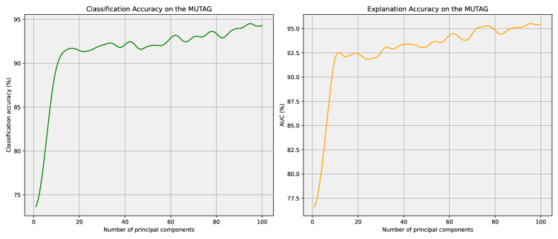
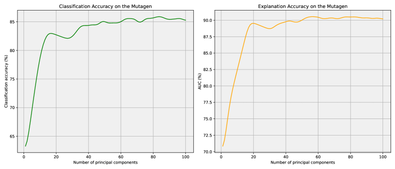
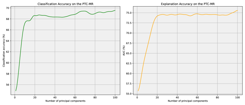
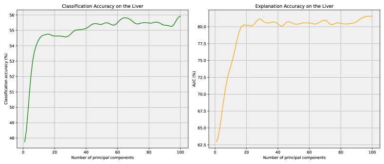
A.9 Does EFPCA effectively works?
In addition to the analysis in section A.8, we demonstrate that the dimensionality reduction by EFPCA effectively preserves the most explanatory components. We compare the model performance (classification accuracy and explanation accuracy) across seven datasets with and without dimensionality reduction. As shown in table 5, when using only 20 principal components, the model performance improves by no more than compared to using all 384 components (i.e., no dimensionality reduction). This indicates that EFPCA effectively preserves the most task-relevant and important information in LLM embeddings while excluding noisy components. These preserved components achieve comparable performance to the models with all components while being significantly simpler and more explainable. This showcases the success of our dimensionality reduction in maintaining model performance while enhancing explainability.
| Dataset | Classification Accuracy () | Explanation Accuracy () |
|---|---|---|
| Mutag | 94.9±1.6 | 96.1±3.0 |
| Mutagen | 86.4±1.4 | 91.2±1.6 |
| PTC-FR | 78.7±1.2 | 82.7±1.7 |
| PTC-FM | 68.1±1.5 | 81.1±2.0 |
| PTC-MR | 70.5±1.7 | 76.5±2.6 |
| PTC-MM | 80.9±2.7 | 75.3±2.2 |
| Liver | 57.3±1.6 | 83.8±1.9 |
A.10 Does The Choice of in N-gram makes a difference?
We compare the different values of in n-gram via cross-validation based on our two evaluation metrics, classification accuracy and explanation accuracy. The results in fig. 6 suggest an overall trend that as goes from 1 to 3, both classification accuracy and explanation accuracy improve; as goes from 4 to 9, both classification accuracy and explanation accuracy drop. On the four datasets we used for experiments, three of them show that good model performance can be achieved when is taken to be 3. As grows from small to large, it encourages the model to capture more contextual semantics, including interactions between functional groups, which allows for a significant improvement in prediction. When exceeds a certain threshold, irrelevant or even toxic information emerges from the captured contextual information (i.e., irrelevant long-range dependencies), making the overall model utility gradually decreases.
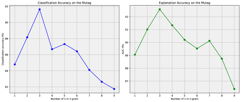
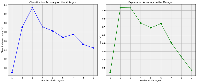
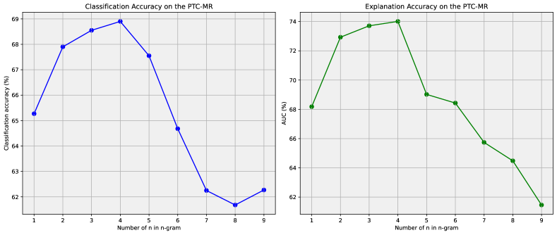
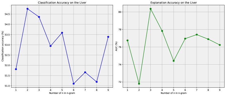
A.11 More explanation visualizations
We randomly select one sample from each of the six remaining datasets and provide explanation visualizations based on MoleX. Specifically, fig. 7, fig. 8, fig. 9, fig. 10, fig. 11, and fig. 12 display the samples selected from the Mutagen, PTC-FM, PTC-MM, PTC-FR, PTC-MR, and Liver datasets, respectively. On the left, we visualize the identified molecular substructures based on different methods, with the ground truth indicating the true substructures influencing molecular properties as given by domain experts. Red marks on the molecular graph highlight important components impacting molecular properties revealed by different methods. We compare with three baselines: OrphicX (Lin et al., 2022), GNNExplainer (Ying et al., 2019), and PGExplainer (Luo et al., 2020), as well as MoleX with and without residual calibration (w/ denotes with and w/o denotes without). On the right, we showcase the n-gram coefficients-based contribution scores of important functional groups revealed by MoleX, ranging from to , where higher scores suggest a more significant contribution to molecular properties.
Taking fig. 7 as an example, MoleX precisely identifies the ground truth substructures for the sample from the Mutagen dataset. Specifically, MoleX highlights the benzene ring bonded with an amino group on the upper left as vital substructures to explain the molecule’s mutagenicity. The contribution scores computed by MoleX indicate that the benzene ring has the highest contribution to molecular properties, followed by the amino group. This aligns with the ground truth that a benzene ring bonded with an amino group leads to mutagenicity (Lin et al., 2022; Debnath et al., 1991). Therefore, MoleX accurately captures the important functional groups (i.e., the benzene ring and the amino group) and the interaction between them, revealing their precise bonding. As the ground truth indicates, only the bonded benzene and amino group together impact the molecular properties. In contrast, other methods provide only atom or bond-level explanations and fail to discover important functional groups as a whole. They identify only a few atoms and bonds in the benzene or amino group and fail to capture the interaction between these two functional groups. Consequently, these atom or bond-level explanations are insufficiently faithful in explaining molecular properties, as individual atoms or bonds have limited impact on overall molecular properties (Mirghaffari et al., 2021). The explanation visualizations for samples from other datasets also demonstrate MoleX’s effectiveness in identifying important substructures and their interactions, aligning with chemical concepts to explain molecular property predictions.
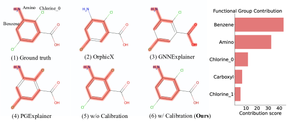
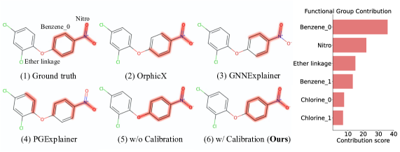
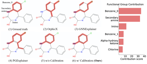
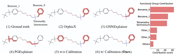
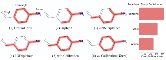
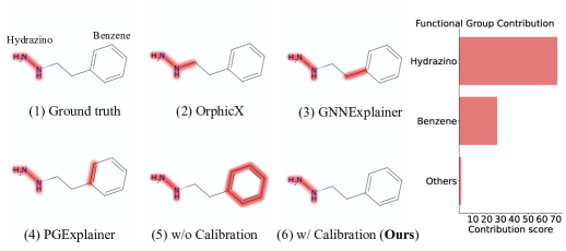
A.12 Can other statistical learning models be augmented with the LLM knowledge?
In addition to the linear model, we augment various statistical learning models with the LLM knowledge and test them on seven datasets. The classification accuracy and explanation accuracy are shown in table 6 and table 7, respectively. Other linear models, such as ridge regression, LASSO, and linear discriminant analysis, achieve comparable performance to MoleX and showcase the generalizability of LLM knowledge augmentation on linear models. Additionally, the polynomial regression, as a more complicated linear model, achieves better performance compared to the simpler ones shown above. For more complex models, such as tree-based and ensemble learning models, the performance is even better, achieving incredible results across all seven datasets. These empirical studies suggest that augmenting statistical machine learning models with LLM knowledge significantly improves performance. Moreover, compared to simple models, the models exhibit more powerful data fitting capabilities become more predictive after the LLM augmentation. However, model complexity generally trades off with explainability. Considering this, we select the logistic regression as our base model due to its optimal balance between explainability and performance.
| Method | Mutag | Mutagen | PTC-FR | PTC-FM | PTC-MR | PTC-MM | Liver |
|---|---|---|---|---|---|---|---|
| Ridge Regression | 90.7±1.2 | 84.1±1.3 | 72.4±2.0 | 65.2±2.0 | 69.8±1.4 | 77.5±1.5 | 58.1±1.6 |
| LASSO | 91.9±1.7 | 84.4±0.7 | 75.1±2.1 | 65.8±1.7 | 65.2±0.9 | 74.2±1.2 | 58.7±1.8 |
| Linear Discriminant Analysis | 89.9±1.9 | 83.6±1.2 | 75.2±1.9 | 65.7±1.9 | 69.3±1.8 | 76.8±2.0 | 57.7±1.3 |
| Polynomial Regression | 93.9±2.4 | 87.2±2.0 | 77.1±2.1 | 67.3±1.8 | 70.2±2.3 | 79.5±1.8 | 60.2±2.4 |
| Support Vector Machine | 93.9±1.6 | 86.6±1.5 | 73.4±1.9 | 69.3±2.6 | 69.5±2.0 | 78.6±1.3 | 61.5±2.9 |
| Decision Tree | 89.7±2.1 | 79.5±1.2 | 72.4±1.8 | 64.3±2.1 | 68.5±1.5 | 74.4±1.4 | 59.5±2.2 |
| Random Forest | 92.8±2.7 | 84.4±1.7 | 77.3±2.1 | 68.6±2.5 | 71.0±2.2 | 77.2±2.1 | 62.7±2.7 |
| Gradient Boosting Machine | 94.8±2.1 | 85.3±1.9 | 78.9±1.9 | 69.4±2.8 | 72.2±2.1 | 79.2±1.9 | 63.9±2.6 |
| XGBoost | 94.6±2.3 | 85.0±2.0 | 78.7±2.2 | 70.1±2.3 | 73.4±2.9 | 78.1±2.1 | 63.0±2.3 |
| MoleX (Ours) | 91.6±2.0 | 83.7±0.9 | 74.4±1.9 | 64.2±1.4 | 68.4±2.3 | 76.4±1.8 | 54.9±2.4 |
| Method | Mutag | Mutagen | PTC-FR | PTC-FM | PTC-MR | PTC-MM | Liver |
|---|---|---|---|---|---|---|---|
| Ridge Regression | 92.8±1.1 | 89.5±1.3 | 79.0±1.2 | 78.1±1.6 | 72.5±2.5 | 69.7±2.3 | 82.4±1.7 |
| LASSO | 92.3±1.5 | 89.6±0.9 | 76.9±1.8 | 81.2±1.9 | 70.4±2.3 | 70.7±2.1 | 81.3±1.8 |
| Linear Discriminant Analysis | 92.9±1.8 | 88.5±1.9 | 80.7±2.3 | 80.1±2.2 | 71.7±2.8 | 71.3±1.6 | 87.8±1.6 |
| Polynomial Regression | 94.3±2.1 | 91.9±1.6 | 80.1±1.9 | 82.9±1.9 | 79.3±2.3 | 75.4±1.7 | 81.0±2.2 |
| Support Vector Machine | 92.0±1.7 | 92.0±1.6 | 84.7±2.2 | 86.3±2.0 | 80.1±2.3 | 76.0±2.3 | 81.9±2.1 |
| Decision Tree | 87.6±1.9 | 89.1±1.5 | 78.6±2.0 | 80.7±1.6 | 73.1±2.1 | 74.2±1.8 | 76.0±1.8 |
| Random Forest | 93.2±1.9 | 90.5±1.8 | 82.1±2.1 | 84.2±2.2 | 74.2±2.0 | 74.5±2.1 | 81.2±2.0 |
| Gradient Boosting Machine | 92.7±2.2 | 92.4±1.5 | 82.9±2.3 | 85.2±2.4 | 73.9±2.9 | 77.7±2.6 | 84.5±2.4 |
| XGBoost | 95.6±1.8 | 90.7±1.7 | 84.0±2.2 | 82.0±2.3 | 74.4±2.7 | 77.4±2.2 | 86.2±2.5 |
| MoleX (Ours) | 92.6±1.7 | 89.0±0.9 | 79.3±2.6 | 77.9±2.6 | 73.4±2.8 | 72.3±3.0 | 80.3±2.5 |
A.13 Classification analysis via Confusion Matrix
As shown in fig. 13, we visualize the classification result via confusion matrix at a random round on the Mutag and PTC-MR datasets. For Mutag, we achieve high precision in predicting the positive class due to fewer false positives and high recall for the positive class, reflecting the model’s effectiveness in identifying positive instances. Furthermore, the model shows a good balance between precision and recall, with a low number of false positives and false negatives. For PTC-MR, the model achieves lower precision compared to the Mutag due to a higher number of false positives. The confusion matrix also suggests that the model struggles with false negatives and false positives, indicating areas for improvement. This analysis highlights the strengths and weaknesses of the model, providing insight for further model refinement.
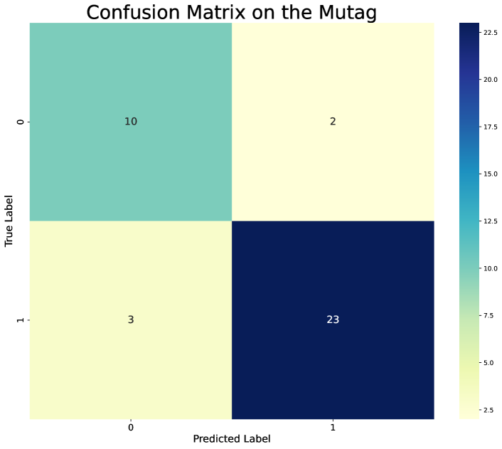
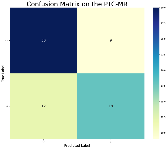
A.14 An illustration of Group SELFIES
As illustrated in fig. 14, the 4-Nitroanisole (\ceC7H7NO3) can be represented by Group SELFIES with three functional groups separated by square brackets: a benzene ring, a nitro group, and a methoxy group (different functional groups are displayed in different colors).
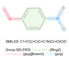
A.15 Broader Impact
This study on explainable molecular property prediction using the LLM-augmented linear model has significant real-world application. The efficiency of linear models allows for fast inference of large-scale molecular data, potentially accelerating drug discovery and materials design processes. This efficiency, combined with the predictive accuracy enhanced by LLM-derived features, and lead to more cost-effective and computationally efficient development in the pharmaceutical and materials industries. The high explanation accuracy of our approach addresses an imperative need in scientific contexts. It provides explainable insights into structure-property relationships, offering faithfulness in predictions and facilitating their adoption in high-stake fields like healthcare. This explainability supports scientific insights, potentially leading to new discoveries in molecular science. Moreover, our method’s balance of predictive accuracy, explainability, and efficiency could serve as a template for developing explainable AI models in other domains, which contributes to the broader goal of trustworthy AI. This could have far-reaching impacts on fields ranging from personalized medicine to sustainable chemistry where understanding the decision-making mechanisms behind predictions is crucial. However, we must also consider potential risks, such as over-reliance on model predictions without appropriate expert validation or the potential misuse in designing harmful molecules. Responsible implementation and research into model limitations are essential.
A.16 Limitations and future works
The proposed explainable molecular property prediction method has some limitations and needs further studies.
-
•
Generalizability: Enhancing the generalizability of explainable models to deal with different molecular datasets across various chemical domains while preserving explainability to structure-property relationships remains a persistent challenge.
-
•
Impact of LLM quality: Though our empirical studies discuss the model performance of Llama3.1 and GPT-4o on molecular property prediction, LLM quality is still a topic that deserves to be explored in-depth. Future studies may discuss how LLM quality impacts the augmented linear model, e.g., model performance change using weak LLMs or LLMs without fine-tuning.
-
•
Trade-off between complexity and performance: In pursuit of explainability, we employ a linear model, which inherently risks underfitting when faced with complex data patterns. Our preliminary experiments comparing MoleX with more sophisticated statistical learning models show marginally better performance from these complex models. Future research could explore the trade-off between model complexity and performance in the context of LLM knowledge augmentation and investigate optimal balances between explainability and performance.