Graph-based identification of qubit network (GidNET) for qubit reuse

Abstract

Quantum computing introduces the challenge of optimizing quantum resources crucial for executing algorithms within the limited qubit availability of current quantum architectures. Existing qubit reuse algorithms face a trade-off between optimality and scalability, with some achieving optimal reuse but limited scalability due to computational complexities, while others exhibit reduced runtime at the expense of optimality. This paper introduces GidNET (Graph-based Identification of qubit NETwork), an algorithm for optimizing qubit reuse in quantum circuits. By analyzing the circuit’s Directed Acyclic Graph (DAG) representation and its corresponding candidate matrix, GidNET identifies higher-quality pathways for qubit reuse more efficiently. Through a comparative study with established algorithms, notably QNET  [1], GidNET not only achieves a consistent reduction in compiled circuit widths by a geometric mean of 4.4%, reaching up to 21% in larger circuits, but also demonstrates enhanced computational speed and scaling, with average execution time reduction of 97.4% (i.e., 38.5$\times$ geometric mean speedup) and up to 99.3% (142.9$\times$ speedup) across various circuit sizes. Furthermore, GidNET consistently outperforms Qiskit in circuit width reduction, achieving an average improvement of 59.3%, with maximum reductions of up to 72% in the largest tested circuits. These results demonstrate GidNET’s ability to improve circuit width and runtime, offering a solution for quantum computers with limited numbers of qubits.

I Introduction

Central to quantum computing is the efficient execution of quantum circuits, a fundamental abstraction underpinning the expression of many quantum algorithms. This necessitates quantum circuit compilation, wherein high-level quantum algorithms are transformed into optimized instructions tailored to a target quantum processor. Essential factors in this optimization include the number of qubits, their connectivity, gate fidelity, and error rates, all aimed at minimizing computational resources and errors during algorithm execution.

At the heart of circuit optimization lies the strategic management of qubits, particularly through their reuse. The innovation of qubit reuse algorithms, which re-purpose qubits in a circuit to a dynamic format requiring fewer resources, marks a significant stride in quantum computing  [2, 1, 3]. This approach, bolstered by the advent of mid-circuit measurement and reset, enhances the scalability and efficiency of computations across both trapped-ion [4] and superconducting systems [5, 6]. Transitioning from static to dynamic quantum circuits, which adjust in real-time to measurement outcomes, qubit reuse is essential across various applications, from error correction [7] and tensor network state preparation [8] to entanglement spectroscopy [9] and quantum machine learning [10]. By mitigating quantum resource demands, it plays a crucial role in overcoming scalability challenges, potentially enhancing circuit fidelity  [11] and reducing complexities  [12]. The industry’s movement towards dynamic circuit capabilities, evidenced by recent hardware enhancements [5, 4], underscores the role of qubit reuse in advancing quantum computing.

The quest for efficient qubit reuse has led to the development of two primary algorithmic approaches: exact algorithms and greedy heuristics  [2]. Exact algorithms, utilizing the Constraint Programming and Satisfiability (CP-SAT) model, offer precision and serve as a valuable benchmark for small-scale systems, albeit with limited scalability. Conversely, greedy heuristic algorithms demonstrate polynomial growth in qubit number and rapid execution times, at the expense of not always achieving optimal results.

In this paper we propose the graph-based identification of qubit network (GidNET) algorithm, a technique to bridge the gap between the exactitude of CP-SAT models and the scalability of greedy heuristics. GidNET leverages the Directed Acyclic Graph (DAG) of a quantum circuit and its matrix representation to identify pathways for qubit reuse. We demonstrate through simulation that, compared to the QNET algorithm in  [1] and the Qiskit implementation of the qubit reuse algorithm in  [2], which we henceforth refer to as Qiskit, GidNET not only achieves a consistent reduction in compiled circuit width but also demonstrates enhanced computational speed. Our contributions are summarized as follows:

• Introduction of ‘reuse sequences’ determined through common neighbors in the circuit’s DAG leading to higher-quality pathways for qubit reuse more efficiently.

• Achievement of consistently reduced compiled circuit widths by a geometric mean of 4.4% and up to 21% in larger circuits, surpassing existing algorithms  [2, 1].

• Significant acceleration of computational runtime over [1], with a geometric mean improvement of 97.4% (or 38.5$\times$), reaching up to 99.3% (142.9$\times$) across different circuit sizes.

• Validation of GidNET’s theoretical complexity through polynomial regression and F-tests, confirming its efficacy against empirical data.

By optimizing qubit reuse, GidNET not only extends the capabilities of existing quantum systems but also reduces operational overhead and is expected to lead to improved quality of circuit execution.

This paper is structured as follows. In Section II, we review existing qubit reuse algorithms and introduce GidNET’s approach. In Section III, we detail the data structures employed by GidNET to facilitate efficient reuse. Section IV describes the algorithm’s implementation and computational complexity. Section V presents the empirical validation of GidNET, demonstrating performance improvements over existing algorithms. Finally, Section VI summarizes our findings and discusses potential future enhancements to GidNET. All the code referenced in this paper is publicly accessible on GitHub

II Related Work and the Novelty of GidNET

In this section, we present quantum circuit cutting and explore existing algorithms for qubit reuse and their limitations, and highlight the unique features of GidNET. We discuss how GidNET leverages graph properties of a quantum circuit to determine reuse, setting it apart from other methods in terms of scalability and performance.

To maximize the utility of current noisy intermediate-scale quantum (NISQ) devices, techniques such as quantum circuit cutting and qubit reuse were developed. Algorithms for circuit cutting split the original quantum circuit either by cutting wires  [13, 14, 15, 16, 17, 18, 19], gates  [20, 21, 22, 23], or both  [24] into smaller subcircuits that can be run separately, either on the same quantum device or on different devices[25]. The results are post-processed and combined using a classical computer. This approach has several drawbacks. For example, the runtime for circuit cutting increases exponentially in the number of cuts on a circuit. In contrast, qubit reuse leverages the ability of a quantum computer to perform mid-circuit measurements and resets, allowing qubit to be reused after they are reset, without necessitating exponential overhead [2].

Recent efforts have focused on algorithms and techniques to enhance qubit reuse and overall quantum circuit efficiency  [2, 1, 3, 26, 27, 28, 29]. Qubit reuse is particularly appealing because promising algorithms for integer factorization  [30], database search  [31], machine learning  [32], and other applications require a large number of qubits. This demand exceeds the capacities of current NISQ computers. The concept of qubit reuse, specifically through wire recycling, was pioneered by Paler et al. [33], emphasizing the underutilization of qubits across quantum circuit computations. This seminal work laid the foundation for subsequent research in qubit reuse strategies. DeCross et al. [2] advanced the field by addressing qubit reuse through mid-circuit measurements and resets, presenting both an exact optimization model and a heuristic for large-scale quantum circuits. Their work highlighted the dual circuit concept, underscoring the symmetry in qubit requirements between a circuit and its temporal reverse. Recent developments by Hua et al. [12] introduced a compiler-assisted tool leveraging dynamic circuit capabilities for qubit reuse. Their empirical analysis demonstrated notable improvements in qubit efficiency and circuit fidelity on actual quantum hardware. Brandhofer et al. [11] proposed an SAT-based model for qubit reuse optimization, tackling the computational challenges inherent in scaling qubit reuse methods. Their approach aims to achieve optimal circuit configurations with respect to various performance metrics, including circuit depth and swap gate insertions.

Most recently, Fang et al. [1] presented a comprehensive study on dynamic quantum circuit compilation, offering the first general framework for optimizing this process through graph manipulation. They formulated the problem using binary integer programming, and introduced algorithms for assessing circuit reducibility and devising dynamic compilation schemes. Their comparative analysis highlights the superior performance of their methods, providing a rigorous foundation for future advances in dynamic circuit compilation  [1].

Building on these works, but particularly inspired by both the complexity of current quantum challenges and the innovative approach by Fang et al.  [1], we propose GidNET, a qubit reuse algorithm that leverages advanced analysis techniques of the quantum circuit’s graph structure, which many of the related works above, apart from QNET [1], do not exploit. Specifically, GidNET utilizes the circuit DAG and the candidate matrix derived from its biadjacency graph. It uniquely determines a greedily-optimized reuse sequence for each qubit, leveraging a property we call common neighbors to methodically select a sequence of qubits for reuse based on interactions between qubits. GidNET ensures that each decision on qubit reuse is informed by a clear understanding of the existing network of qubit relationships, streamlining the application of reuse and improving the outcome of circuit compilation. This strategic approach contrasts with  [1], which broadly evaluates every edge in the candidate matrix to identify the edge that maximizes the possibility of adding more edges in subsequent steps in each iteration.

@C=1.0em @R=0.7em & q_0 : 4 [0em]4
q_1 :
q_2 : 2
q_3 : 1
q_4 :
meas : /__5 __0 @¡= [-5,0] __1 @¡= [-4,0] __2 @¡= [-3,0] __3 @¡= [-2,0] __4 @¡= [-1,0]

(a)

(b)

(c)

Figure 1: (a) A 5-qubit quantum circuit. (b) DAG, $\mathcal{G}$ for the circuit in  1(a). Green nodes are the roots of qubits while violet nodes are terminals of qubits. Blue nodes are CNOT gates between two qubits. (c) Simplified DAG (biadjacency graph) $\mathcal{G}^{\prime}$, derived from  1(b) showing connections from roots ($r$) to terminals ($t$) of qubits. An edge, ($\mathbf{q^{\text{r}}_{i}},\mathbf{q^{\text{t}}_{j}}$) between two qubits indicates a direct path from qubit $\mathbf{q_{{i}}}$ to qubit $\mathbf{q_{{j}}}$ in $\mathcal{G}$, highlighting qubit pairs ineligible for reuse.

III Data Structures

This section summarizes the framework for circuit analysis and qubit reuse introduced by  [1] that is leveraged by GidNET. Given a circuit $\mathcal{Q}$, with set of $n$ qubits $\{\mathbf{q_{{0}}},...,\mathbf{q_{{n-1}}}\}$, the first step is to compute the circuit’s DAG, $\mathcal{G=(V,E)}$, which encapsulates the causal sequence of quantum operations. An example circuit and its DAG are shown in 1(a) and 1(b) respectively. The DAG consists of three types of vertices, $\mathcal{V}$: roots (green), terminals (violet), and operations (blue). The roots are vertices with no incoming edges, representing the first layer of quantum operations on each qubit, usually reset operations. The terminals are vertices with no outgoing edges, representing the last layer of quantum operations, typically quantum measurements. Internal vertices with incoming and outgoing edges correspond to intermediate quantum operations, such as quantum gates. Directed edges between these vertices represent qubits on which these operations are applied.

A circuit DAG can be further simplified to a bipartite graph $\mathcal{G^{\prime}=(R,T,E)}$, where $\mathcal{R}$ and $\mathcal{T}$ denote the sets of roots and terminals from the DAG representation, respectively. An edge $(r,t)\in\mathcal{E}$ connects a root $r\in\mathcal{R}$ to a terminal $t\in\mathcal{T}$ if there exists a directed path from $r$ to $t$ in the original DAG, $\mathcal{G}$. Each $\mathbf{q^{\text{r}}_{i}}$ and $\mathbf{q^{\text{t}}_{i}}$ represent the root and terminal vertices of the $i$-th qubit respectively. The simplified DAG, $\mathcal{G}^{\prime}$ is known as the biadjacency graph  [1].  1(c) shows the biadjacency graph of  1(b), and  2(b) its matrix representation, $\mathfrak{B}$. Row and column indices correspond to the root and terminal nodes of qubits. The biadjacency graph is crucial for the reuse process: if the terminal node of qubit $\mathbf{q_{j}}$ is connected to the root node of qubit $\mathbf{q_{i}}$ in $\mathcal{G}^{\prime}$, the physical qubit associated with $\mathbf{q_{i}}$ cannot be measured and subsequently reused to represent qubit $\mathbf{q_{j}}$ because $\mathbf{q_{j}}$’s operation depends on $\mathbf{q_{i}}$. For instance, in 1(c), qubit $\mathbf{q_{4}}$ cannot reuse qubit $\mathbf{q_{0}}$ due to the edge from root $\mathbf{q^{\text{r}}_{4}}$ to terminal $\mathbf{q^{\text{t}}_{0}}$.

(a)

(b)

(c)

(d)

Figure 2: (a) The biadjacency graph (same as  1(c)). (b) The biadjacency matrix $\mathfrak{B}$, labels rows (root) and columns (terminals) from $\mathbf{q_{{0}}}$ to $\mathbf{q_{{n-1}}}$. (c) The candidate graph is the graph compliment of  2(a). An edge signifies that the root qubit can reuse the terminal qubit post-operation. (d) The candidate matrix $\mathfrak{C}$, as defined in  Equation 1, with rows (terminals) and columns (roots) labeled ($\mathbf{q_{{0}}},...,\mathbf{q_{{n-1}}}$). A ‘1’ indicates a potential reuse opportunity.

To determine which qubits can be reused, we construct a candidate matrix, $\mathfrak{C}$, the adjacency matrix of a candidate graph. Given a biadjacency matrix $\mathfrak{B}$ [1],

$$\mathfrak{C}=\mathbf{1}_{n\times n}-\mathfrak{B}^{T},\vspace{-0.7em}$$ (1)

where $\mathbf{1}_{n\times n}$ is an $n\times n$ all-ones matrix.  2(c) and  2(d) show the candidate graph and matrix of the circuit in 1(a) respectively. The candidate graph is the graph complement of the biadjacency graph where the edges are from the terminals (rows of $\mathfrak{C}$) to the roots (columns of $\mathfrak{C}$). Edges from a given qubit’s terminal are only connected to the roots of qubits that do not share a direct connection with the qubit’s terminal in the biadjacency graph. An edge in the candidate graph from a qubit’s terminal to another qubit’s root indicates that the latter qubit can reuse the former qubit once the former qubit has completed its operation.

IV GidNET Qubit Reuse Algorithm

In this section, we describe GidNET in detail. In  Section IV-B, we explain each operational phase, showcasing its systematic approach to identifying and optimizing qubit reuse sequences using the candidate matrix. In  Section IV-C we analyze the complexity of GidNET.

A qubit reuse algorithm transforms a static quantum circuit, $\mathcal{Q}$, into an equivalent dynamic circuit, $\mathcal{D}$, using fewer qubits, as illustrated in Figure 3. To avoid any ambiguity, we define distinct categories of qubits: logical qubits denoted as $\mathbf{q}$, are those in the original static quantum circuit; virtual qubits denoted as $\mathbf{z}$, are qubits in the transformed dynamic circuit; and physical qubits are actual qubits on quantum hardware.

IV-A Qubit reuse sequence

To explain the intuition behind GidNET, we examine the reuse sequence for each virtual qubit in $\mathcal{D}$.

Definition 1:

Reuse sequence. We define $\mathbb{F}_{\textbf{i}}$, the reuse sequence of virtual qubit $\mathbf{z_{{i}}}$ in a dynamic quantum circuit $\mathcal{D}$, as the sequence of logical qubits $\mathbf{q_{{j}}}$ from the original static circuit $\mathcal{Q}$ that are mapped onto $\mathbf{z_{{i}}}$. The number of virtual qubits in $\mathcal{D}$ is the width of $\mathcal{D}$.

Example 1:

Reuse sequence illustration. The reuse sequences of virtual qubits $\mathbf{z_{0}}$ and $\mathbf{z_{1}}$ in the dynamic circuit $\mathcal{D}$ of  3(b) are $\mathbb{F}_{\textbf{0}}=\{\mathbf{q_{0}},\mathbf{q_{2}},\mathbf{q_{3}},\mathbf{q_{1}}\}$ and $\mathbb{F}_{\textbf{1}}=\{\mathbf{q_{4}}\}$. $\mathcal{D}$ has width 2.

The purpose of GidNET is to compute the longest or most optimized reuse sequences for $\mathcal{D}$ such that its width is minimized. The order of logical qubits in each $\mathbb{F}_{\textbf{i}}$ plays a pivotal role in the quality of the overall solution. To find the optimal set of reuse sequences that results in the smallest circuit width, one could explore all possible sequences that form valid reuse sequences. A valid reuse sequence is one that does not introduce a cycle in the DAG of $\mathcal{D}$. Even though finding the optimal set of reuse sequences may be computationally cheap for a small quantum circuit, it gets prohibitively expensive as circuit size increases.

To reduce the computational cost, GidNET randomly selects from the available logical qubits to determine each $\mathbb{F}_{\textbf{i}}$. This randomness necessitates running the algorithm multiple times, but improves the likelihood of identifying more optimized qubit reuse sequences for $\mathcal{D}$.

IV-B Description of GidNET Algorithm

The GidNET Algorithm  1 employs Algorithm  2 to determine a set of reuse sequences for $\mathcal{D}$. GidNET’s inputs are a circuit, $\mathcal{Q}$, the number of qubits in the circuit, $n$, and the number of iterations, $i$, to run the algorithm. Its output is a set containing the optimized reuse sequences with reduced width for the dynamic circuit $\mathcal{D}$.

Algorithm 1 GidNET Qubit Reuse Algorithm

1:$\mathcal{Q}$, n, i

2:List of qubit reuse sequences

3:$\mathfrak{C}\leftarrow$ Compute the Candidate Matrix of $\mathcal{Q}$

4:$\mathbb{U}\leftarrow$ $\{\{\mathbf{q_{0}}\},\{\mathbf{q_{1}}\},...,\{\mathbf{q_{n-1}}\}\}$

5:if $\forall\mathbf{q^{\text{t}}_{i}},\mathbf{q_{j}}\;(\mathfrak{C}_{\mathbf{q^{\text{t}}_{i}},\mathbf{q_{j}}}=0)$ then

6:     return $\mathbb{U}$ $\triangleright$ Irreducible circuit

7:end if

8:for range($i$) do

9:     $\mathfrak{C^{\prime}}\leftarrow\textsc{Copy}(\mathfrak{C})$

10:     $\mathbb{U}^{\prime}\leftarrow$ { }

11:     while $\sum_{\mathbf{q^{\text{t}}_{i}},\mathbf{q_{j}}}\mathfrak{C^{\prime}}_{\mathbf{q^{\text{t}}_{i}},\mathbf{q_{j}}}>0$ do

12:         $\mathbf{r}[\mathbf{q^{\text{t}}_{i}}]\leftarrow$ sum of rows $\mathbf{q^{\text{t}}_{i}}$ in $\mathfrak{C^{\prime}}$ $\triangleright$ Equation 9

13:         $\mathbb{A}\leftarrow$ $\{\mathbf{q^{\text{t}}_{i}}\}$ rows sums $>0$, $\triangleright$ Equation 8

14:         $\mathbf{q^{\text{t}}_{i}}\leftarrow$ random element from $\mathbb{A}$

15:         $\mathbb{F}_{\textbf{i}},\mathfrak{C^{\prime}}\leftarrow$ $\mathit{BestReuseSequence}$($\mathfrak{C^{\prime}}$, $\mathbf{q^{\text{t}}_{i}}$) $\triangleright$ Algo. 2

16:         if $|\mathbb{F}_{\textbf{i}}|>1$ then

17:              $\mathbb{U^{\prime}}\leftarrow\mathbb{U^{\prime}}\|\mathbb{F}_{\textbf{i}}$

18:         end if

19:     end while

20:     $\mathbb{U}^{\prime}\leftarrow$ $\mathit{MergeSubsets}$($\mathbb{U}^{\prime}$)

21:     $\mathbb{U}^{\prime}\leftarrow$ $\mathit{FinalizeReuse}$($\mathbb{U}^{\prime}$, $n$)

22:     if $|\mathbb{U}^{\prime}|<|\mathbb{U}|$ then

23:         $\mathbb{U}\leftarrow$ $\mathbb{U}^{\prime}$

24:     end if

25:end for

26:return $\mathbb{U}$

Algorithm 1 starts by computing the biadjacency and candidate matrices of the input circuit (line 1) [1]. Line 2 initializes the set of reuse sequences $\mathbb{U}$ with all the qubits in the circuit. Line 3 checks if the candidate matrix is all zeros, indicating an irreducible circuit. If true, line 4 returns $\mathbb{U}$ with all original qubits, as no reuse is possible.

The core of the algorithm is lines 6-23, where reuse sequences for $\mathcal{D}$ are computed. Line 6 ensures this is repeated i times, where $\textit{i}\propto\log(n)$. The choice of $\log(n)$ iterations is empirically driven. After evaluating various options, we found using $\log(n)$ iterations consistently achieved the highest performance across different circuit sizes. Performance was measured based on the likelihood of finding the lowest-width circuit, and the quality of the solution relative to the number of iterations. Using $\log(n)$ iterations provided an optimal balance, ensuring a high probability of success in finding the best circuit while minimizing computational resources.

Lines 7-8 guarantee that each iteration uses a fresh copy of the circuit’s candidate matrix, $\mathfrak{C}^{\prime}$, and creates a new reuse sequence, $\mathbb{U}^{\prime}$. Line 9 ensures the algorithm stops when are no more edges in the candidate matrix. Lines 10 and 11 determine the available qubits from $\mathfrak{C}^{\prime}$ using  Equation 8 and  Equation 9 which are described in Definition 5, while line 12 randomly selects a qubit from the available qubits $\mathbb{A}$ to compute its reuse sequence. Using Algorithm  2, line 13 computes the reuse sequence of the selected qubit and updates the candidate matrix to remove one or more edges accordingly.

After identifying the reuse sequence of the selected qubit, line 14 checks if it is valid (contains more than one qubit). Line 15 appends a valid reuse sequence to the set of reuse sequences for $\mathcal{D}$. In line 18, the algorithm consolidates the reuse sequences by merging subsequences with common qubits that could form a single reuse sequence. Line 19 adds any qubits from the original circuit that lack a reuse sequence (ensuring all qubits are accounted for). Lines 20-22 compare the reuse sequence of the previous iteration to the current iteration, ensuring that the best reuse sequences, i.e., the smallest set, is chosen. A smaller set indicates that more qubits are being reused within fewer sequences, effectively reducing the overall width of the original circuit.

The remainder of this section goes through the details of the most important subroutine in Algorithm 1 more carefully.

IV-B1 The $\mathit{BestReuseSequence}$ Subroutine

The $\mathit{BestReuseSequence}$ subroutine (Algorithm  2) in line 13 of Algorithm 1 computes the reuse sequence, $\mathbb{F}_{\textbf{i}}$, of qubit $\mathbf{q_{{i}}}$ using the candidate matrix, $\mathfrak{C}$.

Algorithm 2 Determine best reuse sequence for qubit $\mathbf{q_{i}}$

1:function BestReuseSequence($\mathfrak{C}$, $\mathbf{q_{i}}$)

2:     $\mathbb{F}_{\textbf{i}}\leftarrow\{\mathbf{q_{i}}\}$

3:     $\mathbb{P}_{\textbf{i}}\leftarrow\{\mathbf{q_{j}}\}$ $\triangleright$ using Equation 2

4:     while $\mathbb{P}_{\textbf{i}}\neq\emptyset$ do

5:         $\boldsymbol{D}\leftarrow\{\}$ $\triangleright$ Placeholder for common neighbors

6:         for $\mathbf{q_{j}}\in\mathbb{P}_{\textbf{i}}$ do

7:              $\boldsymbol{D}[\mathbf{q_{j}}]\leftarrow\mathbb{N}_{\textbf{j}}$ $\triangleright$ using Equations 3 and 4

8:         end for

9:         if $\forall\mathbf{q_{j}}\in\boldsymbol{D},\boldsymbol{D}[\mathbf{q_{j}}]=\emptyset$ then

10:              $\mathbf{q_{j}}\leftarrow$ random element from $\mathbb{P}_{\textbf{i}}$

11:              $\mathbb{F}_{\textbf{i}}\leftarrow\mathbb{F}_{\textbf{i}}\cup\{\mathbf{q_{j}}\}$

12:              $\mathbb{P}_{\textbf{i}}\leftarrow\boldsymbol{D}[\mathbf{q_{j}}]$

13:         else

14:              $\boldsymbol{S}[\mathbf{q_{j}}]\leftarrow I_{\textbf{j}}$ $\triangleright$ using Equations 6, 7, and 4

15:              $\mathbf{q_{j}}\leftarrow\sim\left\{\mathbf{q_{j}}\mid\boldsymbol{S}[\mathbf{q_{j}}]=\max(\boldsymbol{S}),\;\forall\mathbf{q_{j}}\in\boldsymbol{S}\right\}$

16:              $\mathbb{F}_{\textbf{i}}\leftarrow\mathbb{F}_{\textbf{i}}\cup\{\mathbf{q_{j}}\}$

17:              $\mathbb{P}_{\textbf{i}}\leftarrow\boldsymbol{D}[\mathbf{q_{j}}]$

18:         end if

19:     end while

20:     for $k=1$ to $|\mathbb{F}_{\textbf{i}}|-1$ do

21:         $\mathbf{q^{\text{t}}_{k}}\leftarrow\mathbb{F}_{i}[k]$ $\triangleright$ terminal node

22:         $\mathbf{q^{\text{r}}_{k+1}}\leftarrow\mathbb{F}_{i}[k+1]$ $\triangleright$ root node

23:         $\mathfrak{C}\leftarrow\mathit{UpdateCMatrix}(\mathfrak{C},\mathbf{q^{\text{t}}_{k}},\mathbf{q^{\text{r}}_{k+1}})$ $\triangleright$ Algo. 3

24:     end for

25:     return $\mathbb{F}_{\textbf{i}}$, $\mathfrak{C}$

26:end function

Examining the relationship between a qubit reuse sequence and the candidate matrix provides insight into $\mathit{BestReuseSequence}$. This relationship can be explained by highlighting the edges common to both the candidate graph of the static quantum circuit $\mathcal{Q}$ and the simplified DAG, $\mathcal{H}^{\prime}$ of the transformed dynamic circuit $\mathcal{D}$.

@C=1.0em @R=0.7em & q_0 : 4 [0em]4
q_1 :
q_2 : 2
q_3 : 1
q_4 :
meas : /__5 __0 @¡= [-5,0] __1 @¡= [-4,0] __2 @¡= [-3,0] __3 @¡= [-2,0] __4 @¡= [-1,0]

(a) The original circuit, $\mathcal{Q}$

@C=0.8em @R=2.9em & z_0 ↦q_0 : 1 q_2 : 1 q_3 : 1 q_1 :
z_1 ↦q_4 :
meas : /__5 __0 @¡= [-2,0] __2 @¡= [-2,0] __3 @¡= [-2,0] __1 @¡= [-2,0] __4 @¡= [-1,0]

(b) The transformed dynamic circuit, $\mathcal{D}$

(c) The simplified DAG, $\mathcal{H}^{\prime}$.

Figure 3: (a) The original circuit $\mathcal{Q}$ uses 5 logical qubits ($\mathbf{q_{0}}\ldots\mathbf{q_{4}}$), whereas the dynamic circuit $\mathcal{D}$ in (b) uses just 2 virtual qubits ($\mathbf{z_{0}},\mathbf{z_{1}}$), at the expense of additional depth. (c) The simplified DAG $\mathcal{H}^{\prime}$ depicts only qubit connections, omitting gate operations. It shows two reuse sequences. The first starts at $\mathbf{q_{0}}$ and passes through $\mathbf{q_{2}},\mathbf{q_{3}},\mathbf{q_{1}}$. The red lines are added to facilitate identification of the qubit reuse sequence. The second is a direct path for $\mathbf{q_{4}}$, with no intermediate qubits.

Example 2:

Reuse sequence versus candidate matrix. The simplified DAG $\mathcal{H}^{\prime}$ in  3(c) has two distinct paths:

1. $\mathbf{q^{\text{r}}_{0}}\rightarrow\mathbf{q^{\text{t}}_{0}}\rightarrow\mathbf{q^{\text{r}}_{2}}\rightarrow\mathbf{q^{\text{t}}_{2}}\rightarrow\mathbf{q^{\text{r}}_{3}}\rightarrow\mathbf{q^{\text{t}}_{3}}\rightarrow\mathbf{q^{\text{r}}_{1}}\rightarrow\mathbf{q^{\text{t}}_{1}}$

2. $\mathbf{q^{\text{r}}_{4}}\rightarrow\mathbf{q^{\text{t}}_{4}}$

They correspond to the reuse sequences, $\mathbb{F}_{\textbf{0}}$ and $\mathbb{F}_{\textbf{1}}$ of virtual qubits $\mathbf{z_{{0}}}$ and $\mathbf{z_{{1}}}$ respectively, in the dynamic circuit $\mathcal{D}$. In this representation, each qubit is replaced by a connection from its root to its terminal, indicating when the qubit was initialized and measured, respectively.

In the first path, the edges common to both the candidate graph in  2(c) and $\mathcal{H}^{\prime}$ in  3(c) are the red-colored edges, $(\mathbf{q^{\text{t}}_{0}},\mathbf{q^{\text{r}}_{2}})$, $(\mathbf{q^{\text{t}}_{2}},\mathbf{q^{\text{r}}_{3}})$ and $(\mathbf{q^{\text{t}}_{3}},\mathbf{q^{\text{r}}_{1}})$, connecting the terminal of one qubit to the root of another qubit in $\mathcal{H}^{\prime}$. Each edge is an entry in the candidate matrix $\mathfrak{C}$. The unique set of logical qubits $\{\mathbf{q_{{0}}},\mathbf{q_{{2}}},\mathbf{q_{{3}}},\mathbf{q_{{1}}}\}$ constituting these edges correspond to the qubits in $\mathbb{F}_{\textbf{0}}$, the reuse sequence of virtual qubit $\mathbf{z_{{0}}}$. The second path in $\mathcal{H}^{\prime}$ has no edge going from the terminal of a qubit to the root of another qubit. Hence, only qubit $q_{\textbf{4}}$ is in $\mathbb{F}_{\textbf{1}}$, the reuse sequence of virtual qubit $\mathbf{z_{{1}}}$.

Example  2 shows that the set of edges from terminals to roots of any reuse sequence, $\mathbb{F}_{\textbf{i}}$, is a subset of edges in the candidate graph and hence, the candidate matrix. This means that we can determine any $\mathbb{F}_{\textbf{i}}$ from $\mathfrak{C}$. However, determining the edges that form $\mathbb{F}_{\textbf{i}}$ from the candidate matrix is challenging. Finding an exact solution involves non-convex optimization that would require $O(n^{2})$ variables and $O(n^{4})$  [1, 2] constraints, making it impractical for large candidate matrices. $\mathit{BestReuseSequence}$ begins by identifying the sets of qubits that can form a potential reuse sequence in the candidate matrix (line 3 of Algorithm 2).

Definition 2:

Potential reuse sequence. We define the potential reuse sequence, $\mathbb{P}_{\textbf{i}}$, as the set of logical qubits that can form a reuse sequence with logical qubit $\mathbf{q_{{i}}}$,

$$\mathbb{P}_{\textbf{i}}=\{\mathbf{q_{{j}}}\mid\mathfrak{C}_{\mathbf{q^{\text{t}}_{i}},\mathbf{q_{j}}}=1,\;\forall j\in\{0,1,\ldots,n-1\}\}.$$ (2)

Example 3:

Potential reuse sequence illustration. To find $\mathbb{P}_{\textbf{0}}$ of the candidate matrix in  2(d), we examine row $\mathbf{q^{\text{t}}_{0}}$ of $\mathfrak{C}$ and its columns $\mathbf{q_{j}}$. The columns indexed by $\mathbf{q^{\text{r}}_{1}}$, $\mathbf{q^{\text{r}}_{2}}$, and $\mathbf{q^{\text{r}}_{3}}$, where the entry in row $\mathbf{q^{\text{t}}_{0}}$ is 1, form this set. Thus, $\mathbb{P}_{\textbf{0}}=\{\mathbf{q_{1}},\mathbf{q_{2}},\mathbf{q_{3}}\}$. This indicates that qubits $\mathbf{q_{1}}$, $\mathbf{q_{2}}$, and $\mathbf{q_{3}}$ could each potentially reuse $\mathbf{q_{0}}$ after $\mathbf{q_{0}}$ completes its operations and could form a potential reuse sequence with $\mathbf{q_{0}}$.

The set $\mathbb{P}_{\textbf{i}}$ is important because for any reuse sequence, $\mathbb{F}_{\textbf{j}}$, that begins with logical qubit $\mathbf{q_{{i}}}$, all other qubits in that sequence must be contained in $\mathbb{P}_{\textbf{i}}$. This is because there is no path in the DAG $\mathcal{G}$, from $\mathbf{q_{{i}}}$ to any $\mathbf{q_{{j}}}\in\mathbb{P}_{\textbf{i}}$ in the original circuit.

The next step is to identify qubits in $\mathbb{P}_{\textbf{i}}$ that form the entries in $\mathbb{F}_{\textbf{j}}$ and in what order. The constraint, however, is that the reuse sequence must be acyclic, i.e., no qubit can appear in $\mathbb{F}_{\textbf{j}}$ twice. To ensure this, any qubit $\mathbf{q_{{k}}}$ added to $\mathbb{F}_{\textbf{j}}$ after qubit $\mathbf{q_{{j}}}$ must not have a pre-existing connection in $\mathcal{G}^{\prime}$ to $\mathbf{q_{{j}}}$, or to any qubit preceding $\mathbf{q_{{j}}}$ in $\mathbb{F}_{\textbf{j}}$. This condition is satisfied if the entry ($\mathbf{q^{\text{t}}_{j}},\mathbf{q^{\text{r}}_{k}}$) in the candidate matrix is 1.

Any of the qubits in $\mathbb{P}_{\textbf{i}}$ can be selected to be the first entry of $\mathbb{F}_{\textbf{j}}$. However, to determine which $\mathbf{q_{j}}\in\mathbb{P}_{\textbf{i}}$ will have the longest reuse sequence while maintaining the acyclicity constraint, we compute the common neighbors, $\mathbb{N}_{\textbf{x}}$ for each $\mathbf{q_{x}}\in\mathbb{P}_{\textbf{i}}$ and select the qubit whose $\mathbb{N}_{\textbf{x}}$ has the maximum size, $|\mathbb{N}_{\textbf{x}}|$.

Definition 3:

Common Neighbors. We define $\mathbb{N}_{\textbf{x}}$, the common neighbors of qubit $\mathbf{q_{x}}$ as:

$$\mathbb{N}_{\textbf{x}}=\bigcap_{\mathbf{q_{k}}\in\mathbb{T}_{\textbf{x}}}\mathbb{P}_{\textbf{k}},$$ (3)

where

$$\mathbb{T}_{\textbf{x}}=\{\mathbb{F}_{\textbf{j}}\cup\{\mathbf{q_{x}}\}\}$$ (4)

is the updated reuse sequence.

The $\mathbb{N}_{\textbf{x}}$ with the maximum size is chosen because it contains more qubits to select from, increasing the likelihood of finding the longest path.

Example 4:

Common neighbors illustration. Recall that in  example 3, we computed $\mathbb{P}_{\textbf{0}}=\{\mathbf{q_{1}},\mathbf{q_{2}},\mathbf{q_{3}}\}$. To determine the optimized $\mathbb{F}_{\textbf{0}}$ that could be derived from $\mathbb{P}_{\textbf{0}}$, we

1. Initialize $\mathbb{F}_{\textbf{0}}=\{\mathbf{q_{0}}\}$

2. Using  Equation 2 compute $\mathbb{P}_{\textbf{i}}$ for each $\mathbf{q_{x}}\in\mathbb{P}_{\textbf{0}}$ as: $\mathbb{P}_{\textbf{1}}=\{\mathbf{q_{0}},\mathbf{q_{2}},\mathbf{q_{3}},\mathbf{q_{4}}\}$, $\mathbb{P}_{\textbf{2}}=\{\mathbf{q_{1}},\mathbf{q_{3}}\}$ and $\mathbb{P}_{\textbf{3}}=\{\mathbf{q_{1}}\}$

3. Using Equation 3 and  Equation 2, compute $\mathbb{N}_{\textbf{x}}$ for each $\mathbf{q_{x}}\in\mathbb{P}_{\textbf{0}}$:

   • For $\mathbf{q_{1}}$:

     $$\mathbb{T}_{\textbf{1}} = \mathbb{F}_{\textbf{0}}\cup\{\mathbf{q_{1}}\}=\{\mathbf{q_{0}},\mathbf{q_{1}}\},$$

     $$\mathbb{N}_{\textbf{1}} = \mathbb{P}_{\textbf{0}}\cap\mathbb{P}_{\textbf{1}}=\{\mathbf{q_{2}},\mathbf{q_{3}}\}.$$

   • For $\mathbf{q_{2}}$:

     $$\mathbb{T}_{\textbf{2}} = \mathbb{F}_{\textbf{0}}\cup\{\mathbf{q_{2}}\}=\{\mathbf{q_{0}},\mathbf{q_{2}}\},$$

     $$\mathbb{N}_{\textbf{2}} = \mathbb{P}_{\textbf{0}}\cap\mathbb{P}_{\textbf{2}}=\{\mathbf{q_{1}},\mathbf{q_{3}}\}.$$

   • For $\mathbf{q_{3}}$:

     $$\mathbb{T}_{\textbf{3}} = \mathbb{F}_{\textbf{0}}\cup\{\mathbf{q_{3}}\}=\{\mathbf{q_{0}},\mathbf{q_{3}}\},$$

     $$\mathbb{N}_{\textbf{3}} = \mathbb{P}_{\textbf{0}}\cap\mathbb{P}_{\textbf{3}}=\{\mathbf{q_{1}}\}.$$

4. Compute the size of each $\mathbb{N}_{\textbf{x}}$: $|\mathbb{N}_{\textbf{1}}|=|\mathbb{N}_{\textbf{2}}|=2$, $|\mathbb{N}_{\textbf{3}}|=1$.

Example 4 shows multiples $\mathbb{N}_{\textbf{x}}$ can have the same maximum size. One option is to randomly select one of them, but this may result in sub-optimal reuse sequences. Instead, we define a secondary quality metric, which we denote as the reuse score.

Definition 4:

Reuse score. We define the reuse score, $I_{\textbf{j}}$, of qubit $\mathbf{q_{j}}$ as:

$$I_{\textbf{j}}=\sum_{\left\{\textbf{j}\neq\textbf{k},\;\forall\mathbf{q_{j}}\in\mathbb{M}\right\}}{\left|\mathbb{N}_{\textbf{j}}\cap\mathbb{N}_{\textbf{k}}\right|},$$ (5)

where

$$\mathbb{M}=\left\{\mathbf{q_{j}}\mid\left|\mathbb{N}_{\textbf{j}}\right|=s,\;\forall\mathbf{q_{j}}\in\mathbb{P}_{\textbf{i}}\right\},$$ (6)

and

$$s=\max\left(\left\{\left|\mathbb{N}_{\textbf{j}}\right|,\;\forall\mathbf{q_{j}}\in\mathbb{P}_{\textbf{i}}\right\}\right)$$ (7)

is the maximum size of any set of common neighbors.

The qubit with the highest $I_{\textbf{j}}$ is chosen because it has a greater influence on the reuse sequence, $\mathbb{F}_{\textbf{j}}$, compared to other qubits. Here, influence means $\mathbf{q_{j}}$ has greater potential to further extend $\mathbb{F}_{\textbf{j}}$ if chosen, because of its $\mathbb{N}_{\textbf{x}}$. If multiple qubits have the same $I_{\textbf{j}}$, one of them is selected at random.

Example 5:

Reuse score illustration. Given that $|\mathbb{N}_{\textbf{1}}|=|\mathbb{N}_{\textbf{2}}|$, we compute $I_{\textbf{j}}$ for each qubit,

$$I_{\textbf{1}}=\sum\left\{\left|\mathbb{N}_{\textbf{1}}\cap\mathbb{N}_{\textbf{2}}\right|\right\}=1,\quad I_{\textbf{2}}=\sum\left\{\left|\mathbb{N}_{\textbf{2}}\cap\mathbb{N}_{\textbf{1}}\right|\right\}=1.$$

Since both qubits have the same reuse score, we can randomly choose one to extend $\mathbb{F}_{\textbf{0}}$. Suppose $\mathbf{q_{2}}$ is selected. Then

$$\mathbb{F}_{\textbf{0}}=\mathbb{T}_{\textbf{2}}=\{\mathbf{q_{0}},\mathbf{q_{2}}\}.$$

For every qubit $\mathbf{q_{j}}$ selected from $\mathbb{P}_{\textbf{i}}$ and appended to $\mathbb{F}_{\textbf{i}}$, the $\mathbb{N}_{\textbf{x}}$ of the selected qubit $\mathbf{q_{j}}$ becomes the updated $\mathbb{P}_{\textbf{i}}$. The set $\mathbb{P}_{\textbf{i}}$ is iteratively updated with $\mathbb{N}_{\textbf{x}}$ after each selection of $\mathbf{q_{j}}$ from $\mathbb{P}_{\textbf{i}}$ until no further qubits can be added to $\mathbb{F}_{\textbf{i}}$ from $\mathbb{P}_{\textbf{i}}$.

Example 6:

Reuse sequence computation. Having determined $\mathbb{F}_{\textbf{0}}=\{\mathbf{q_{0}},\mathbf{q_{2}}\}$, and $\mathbb{P}_{\textbf{0}}$ is updated to $\mathbb{P}_{\textbf{0}}=\mathbb{N}_{\textbf{2}}=\left\{\mathbf{q_{1}},\mathbf{q_{3}}\right\}$, we want to select the next qubit from the updated $\mathbb{P}_{\textbf{0}}$. Following the steps in  example 4, we have:

1. Using equations Equation 3 and  Equation 2, we compute $\mathbb{N}_{\textbf{x}}$ for each $\mathbf{q_{x}}\in\mathbb{P}_{\textbf{0}}$

   • For $\mathbf{q_{1}}$:

     $$\mathbb{T}_{\textbf{1}} = \mathbb{F}_{\textbf{0}}\cup\{\mathbf{q_{1}}\}=\{\mathbf{q_{0}},\mathbf{q_{2}},\mathbf{q_{1}}\},$$

     $$\mathbb{N}_{\textbf{1}} = \mathbb{P}_{\textbf{0}}\cap\mathbb{P}_{\textbf{2}}\cap\mathbb{P}_{\textbf{1}}=\{\mathbf{q_{3}}\}.$$

   • For $\mathbf{q_{3}}$:

     $$\mathbb{T}_{\textbf{3}} = \mathbb{F}_{\textbf{0}}\cup\{\mathbf{q_{3}}\}=\{\mathbf{q_{0}},\mathbf{q_{2}},\mathbf{q_{3}}\},$$

     $$\mathbb{N}_{\textbf{3}} = \mathbb{P}_{\textbf{0}}\cap\mathbb{P}_{\textbf{2}}\cap\mathbb{P}_{\textbf{3}}=\{\mathbf{q_{1}}\}.$$

2. compute the size of each $\mathbb{N}_{\textbf{x}}$: $|\mathbb{N}_{\textbf{1}}|=1$ and $|\mathbb{N}_{\textbf{3}}|=1$.

Both $\mathbf{q_{1}}$ and $\mathbf{q_{3}}$ have the same $|\mathbb{N}_{\textbf{x}}|=1$. Computing $I_{\textbf{j}}$ for each yields $I_{\textbf{1}}=I_{\textbf{3}}=0$. This means we can randomly select either $\mathbf{q_{1}}$ or $\mathbf{q_{3}}$ to append to $\mathbb{F}_{\textbf{0}}$. Suppose $\mathbf{q_{3}}$ is randomly selected, resulting in $\mathbb{F}_{\textbf{0}}=\{\mathbf{q_{0}},\mathbf{q_{2}},\mathbf{q_{3}}\}$, then the updated $\mathbb{P}_{\textbf{0}}=\mathbb{N}_{\textbf{3}}=\{\mathbf{q_{1}}\}$. Since there is only one element left in $\mathbb{P}_{\textbf{0}}$, we append it to $\mathbb{F}_{\textbf{0}}$ and obtain $\mathbb{F}_{\textbf{0}}=\{\mathbf{q_{0}},\mathbf{q_{2}},\mathbf{q_{3}},\mathbf{q_{1}}\}$ and $\mathbb{P}_{\textbf{0}}=\emptyset$. This completes the reuse sequence $\mathbb{F}_{\textbf{0}}$ of qubit $\mathbf{q_{{0}}}$.

Algorithm 3 Update Candidate Matrix After Selection

1:procedure UpdateCMatrix($\mathfrak{C}$, $\mathbf{q^{\text{t}}_{i}}$ , $\mathbf{q_{j}}$)

2:     $\mathbb{V}_{r}\leftarrow\{\mathbf{q^{\text{r}}_{k}}\,|\,\mathfrak{C}_{\mathbf{q^{\text{t}}_{i}},\mathbf{q^{\text{r}}_{k}}}=0,\;\forall k\in\{0,1,\ldots,n-1\}\}$

3:     $\mathbb{V}_{t}\leftarrow\{\mathbf{q^{\text{t}}_{k}}\,|\,\mathfrak{C}_{\mathbf{q^{\text{t}}_{k}},\mathbf{q_{j}}}=0,\;\forall k\in\{0,1,\ldots,n-1\}\}$

4:     for $(\mathbf{q^{\text{t}}_{k}},\mathbf{q^{\text{r}}_{l}})\in\{\mathbb{Q}_{t}\}\times\{\mathbb{Q}_{r}\}$ do

5:         $\mathfrak{C}_{\mathbf{q^{\text{t}}_{k}},\mathbf{q^{\text{r}}_{l}}}\leftarrow 0$

6:     end for

7:     $\mathfrak{C}_{\mathbf{q^{\text{t}}_{i}},\mathbf{q^{\text{r}}_{k}}}\leftarrow 0,\;\forall k\in\{0,1,\ldots,n-1\}$

8:     $\mathfrak{C}_{\mathbf{q^{\text{t}}_{k}},\mathbf{q_{j}}}\leftarrow 0,\;\forall k\in\{0,1,\ldots,n-1\}$

9:     return $\mathfrak{C}$

10:end procedure

After the reuse sequence of a qubit is determined, the $\mathit{UpdateCMatrix}$ procedure in algorithm  3 updates the candidate matrix, as done in  [1]. This is crucial to avoid multiple selections of an edge. It also prevents the creation of cycles in the DAG and eliminates potential conflicts in qubit reuse. It is possible that edges remain in the candidate matrix after the update; this signals more qubit reuse opportunities. In this case, a new set of available qubits is derived from the updated candidate matrix.

Definition 5:

Available qubits. We define the available qubits in the candidate matrix as follows:

$$\mathbb{A} = \{\mathbf{q_{i}}\mid\mathbf{r}[\mathbf{q_{i}}]>0,\;\forall\text{i}\in\{0,1,\ldots,n-1\}\}$$ (8)

where $\mathbf{r}$ is the sum of each row in $\mathfrak{C}$,

$$\mathbf{r}[\mathbf{q_{i}}] = \sum_{\textbf{j}=0}^{n-1}\mathfrak{C^{\prime}}_{\mathbf{q^{\text{t}}_{i}},\mathbf{q_{j}}}\quad\forall\text{i}\in\{0,1,\ldots,n-1\}.$$ (9)

Upon confirming availability of additional qubits, another qubit is selected, its reuse sequence computed, and the candidate matrix updated. This process is repeated until no edges remain in the candidate matrix (line 23 of Algorithm  2).

IV-C Complexity Analysis of the GidNET Qubit Reuse Algorithm

The time complexity of initializing variables and computing matrices for a quantum circuit depends on its size. Given a circuit with $n$ qubits and $m$ gates, it is converted into a DAG in $O(m)$ time, then simplified using Depth First Search (DFS). Running DFS to determine an edge $(\mathbf{q^{\text{r}}_{j}},\mathbf{q^{\text{t}}_{i}})$ in the biadjacency graph $\mathcal{G}^{\prime}$ has complexity $O(m)$. In $\mathcal{G}^{\prime}$, there are at most $n^{2}$ edges from roots $\mathbf{q^{\text{r}}_{j}}$ to terminals $\mathbf{q^{\text{t}}_{i}}$, resulting in an overall complexity of $O(mn^{2})$. Computing the biadjacency matrix from $\mathcal{G}^{\prime}$, and then the candidate matrix, both take $O(n^{2})$.

After determining the optimized reuse sequence $\mathbb{U}$, the DAG is converted to a dynamic circuit. For dynamic circuit conversion, edges are added to the DAG from $\mathbb{U}$, requiring $O(m)$ for topological sorting and another $O(m)$ for appending instructions. The final step of updating instructions for each qubit takes $O(mn)$, resulting in a total time complexity of $O(m)+O(m)+O(mn)=O(mn)$. Hence, the total time complexity for data structure creation and postprocessing is $O(m)+O(n^{2})+O(mn^{2})+O(mn)=O(mn^{2})$.

Next, we examine lines 6-17 of Algorithm  1. For each of the $\log n$ iterations (line 6), the algorithm iterates over the available qubits $\mathbb{A}$ in the candidate matrix (line 11) to randomly select a qubit (line 12), leading to an outer loop complexity that scales as $O(\log n)$. At each iteration, the candidate matrix is duplicated to preserve its original state for subsequent evaluations (line 7); this involves $O(n^{2})$ operations to replicate each matrix element. A significant portion of the algorithm is spent in a while loop (lines 9-17), determining potential reuse sequences (see  Section IV-A) until exhaustion. The sum operation within this loop, necessary to evaluate the continuation condition (line 9), exhibits $O(n^{2})$ complexity per iteration. The progressive reduction of viable qubits reduces the computational load of subsequent iterations.

The invocation of $\mathit{BestReuseSequence}{}$  2 (line 13) constitutes the algorithmic core, tasked with identifying the most efficient reuse sequence for a selected qubit. This function’s complexity, preliminarily estimated at $O(n^{3})$ (see  Section IV-C1), dominates the overall computational effort, attributed to extensive matrix operations and sequence updates. Assuming the main loop iterates $p$ times, where $p<n$, the cumulative complexity approximates to $O(p\cdot n^{3})$. Post-calculation, the algorithm merges overlapping sequences and adjusts the reuse list to include all qubits. $\mathit{MergeSubsets}{}$ (line 18) merges pairs of elements in the final reuse sequence into interconnected subsequences, ensuring all elements connected directly or indirectly are in the same subsequence. This involves iteratively checking and merging pairs with a function that finds a common subsequence for a given pair, and another function that merges two subsequences while maintaining their order. The merging process, including additional passes to ensure all interconnected subsequences are fully merged, yields a time complexity of $O(\mu\times\nu\times k^{2})$, where $\mu$ is the number of pairs, $\nu$ is the number of merged subsequences, and $k$ is the average length of each subsequence.

FinalizeReuse (line 19) ensures all qubits are accounted for. It first creates a set of all qubits in the current reuse sequence, then compares this to a set of the original qubits ($n$) to find any missing qubits. Missing qubits are appended as individual elements to the set of reuse sequences. This guarantees that every qubit is present, either as part of a reuse sequence or independently, resulting in a complete and finalized qubit reuse list. The time complexity is $O(n)$.

Considering the algorithm’s iterative nature and the significant impact of converting the circuit DAG to simplified DAG, the $\mathit{BestReuseSequence}{}$ function, and $\mathit{MergeSubsets}{}$ the cumulative complexity of GidNET can be conservatively approximated as $O(mn^{2}+\mu\nu k^{2}+pn^{3}\log{n})$.

IV-C1 Complexity Analysis of BestReuseSequence Function

The $\mathit{BestReuseSequence}$ function (Algorithm  2) is pivotal in determining the optimal reuse sequence for a qubit $\mathbf{q^{\text{t}}_{i}}$. Initialization of $\mathbb{F}_{\textbf{i}}$ (line 2) and $\mathbb{P}_{\textbf{i}}$ (line 3) are $O(1)$ and $O(n)$ operations respectively. In lines 4-19, the while loop iterates over potential qubits in $\mathbb{P}_{\textbf{i}}$ until no further qubits can be added to $\mathbb{F}_{\textbf{i}}$, potentially engaging with all $n$ qubits in $\mathbb{P}_{\textbf{i}}$. Inside the while loop, for each qubit, $\mathbf{q_{j}}$ in the current $\mathbb{P}_{\textbf{i}}$, $\mathbb{N}_{\textbf{j}}$ is computed and stored in the placeholder $\boldsymbol{D}$. Each $\mathbb{N}_{\textbf{j}}$ requires $O(n)$ complexity. Thus, the for loop runs in $O(n)\times O(n)=O(n^{2})$ to compute all $\mathbb{N}_{\textbf{j}}$.

Lines 9-12 handle the case where all computed $\mathbb{N}_{\textbf{j}}$ in $\boldsymbol{D}$ are empty, which involves checking if all values in $\boldsymbol{D}$ are empty, in time $O(n)$. Lines 13-18 are the cases where at least one $\mathbb{N}_{\textbf{j}}$ is not empty and multiple qubits, $\mathbf{q_{j}}$ have maximum $\mathbb{N}_{\textbf{j}}$. Finding the placeholder $\boldsymbol{S}$ in line 14 using Equations 6, 7, and 4 involves iterating over each $\mathbf{q_{j}}$ in $\mathbb{M}$. During each iteration, it computes intersections with $O(n)$ complexity, calculates the sum of intersections with $O(n)$ complexity and updates $\boldsymbol{S}$ with $O(1)$ complexity. This results in a total complexity of $O(n)\times(O(n)+O(n)+O(1))=O(n^{2})$. Line 15 has $O(n)$ complexity, while each update in lines 16-17 requires $O(1)$ complexity. Hence, the dominant time complexity of lines 9-18 is $O(n^{2})$.

Finally, lines 20-24 call $\mathit{UpdateCMatrix}$ to update $\mathfrak{C}$ if $|\mathbb{F}_{\textbf{i}}|>1$. Each call to $\mathit{UpdateCMatrix}$ is $O(n^{2})$ (see Algorithm  3 in  Section IV-C2), and the loop runs up to $n$ times giving a total complexity of $O(n^{2})\times O(n)=O(n^{3})$. Thus, the overall time complexity of the $\mathit{BestReuseSequence}$ is $O(n^{2})+O(n^{3})+O(n^{2})+O(n^{3})=O(n^{3})$.

IV-C2 Complexity Analysis of Update Candidate Matrix After Selection

The function updates the matrix based on a chosen qubit’s terminal $\mathbf{q^{\text{t}}_{i}}$ and another qubit’s root $\mathbf{q^{\text{r}}_{j}}$. Identifying nodes not directly connected to $\mathbf{q^{\text{t}}_{i}}$ and $\mathbf{q_{j}}$ requires examining each element along a specified row and column, which is $O(n)$ overall. Setting an entire row and column to zero is also $O(n)$. The most intensive task is the nested loop that runs for all pairs in the Cartesian product of the set of root vertices $\mathbb{V}_{r}$, and the set of terminal vertices $\mathbb{V}_{t}$ (lines 4-6), updating the matrix to account for indirect connections and possibly requiring a review and update of every matrix entry. This step dominates, leading to an overall complexity of $O(n^{2})$.

V Experimental Setup and Results

In this section, we present the experimental setup, benchmarking results, and the statistical methods used to validate the performance improvements of GidNET.

Two qubit reuse algorithms were compared against GidNET: QNET  [1], and the Qiskit implementation  [34] of the qubit reuse algorithm in  [2]. Due to the proprietary implementation of  [2], direct access was unavailable as it requires a subscription to Quantinuum’s H-series hardware . The authors provided detailed insights into the algorithm’s principles for academic understanding. For our study, we assume the Qiskit implementation reflects the original algorithm’s functionality.

Experimental validation of GidNET was conducted on a set of benchmark circuits, including both Google random circuit sampling (GRCS) and Quantum Approximate Optimization Algorithm (QAOA) circuits. We specifically chose these circuits because they were used in prior works to assess qubit reuse algorithms on near-term quantum devices [2, 1].

Benchmarks were conducted on a virtual machine hosted by an Acer Nitro N50-640 desktop running Windows 11 x64. The host system was equipped with a 12th Gen Intel(R) Core(TM) i7-12700F 2.10 GHz processor and 16 GB of RAM. Virtualization was facilitated by VMware Workstation 17, which ran an Ubuntu 22.04.1 LTS virtual machine. The VM was configured with 8 CPU cores, 16 GB of RAM.

To assess the runtime efficiency of GidNET, QNET, and Qiskit, "%timeit -o" command was employed within a JupyterLab notebook environment. While it is acknowledged that high-performance computing resources could potentially enhance the feasibility range of the tested algorithms, the results presented herein aim to approximate the conditions accessible to most researchers and developers.

To ensure consistency, each randomly generated circuit was seeded such that each algorithm operated on identical circuit configurations. Performance data collected from the application of the three algorithms was analyzed to determine their efficacy. Runtime and circuit width before and after application of each algorithm were recorded. Statistical tests using polynomial regression were employed to validate the theoretically obtained complexity analyses of GidNET and QNET against experimental results.

V-A Google Random Circuit Sampling (GRCS)

GRCS was introduced to demonstrate quantum computers’ capability to solve problems intractable for classical computers, using random quantum circuits  [35]. GRCS utilizes circuits designed for qubits arranged in an $n_{1}\times n_{2}$ lattice, which incorporates several cycles of quantum gates on all qubits. First, a layer of Hadamard gates is applied across all qubits. Subsequent cycles include a structured pattern: a layer of controlled $Z$ ($CZ$) alternately arranged according to some pre-defined patterns, succeeded by a layer of single-qubit gates—$\{X^{1/2},Y^{1/2},T\}$—targeted at qubits not involved in the $CZ$ gates during the same cycle.

GRCS circuits with 16 to 144 qubits were generated at depths 11, 12, and 15 for each qubit number. The performance of the algorithms was evaluated based the reduction in circuit width and the overall runtime.

Due to the random nature of GidNET and QNET, each GRCS circuit was benchmarked 10 times, and the best (or smallest) compiled circuit width recorded. Qiskit was only run once for each circuit since it is a deterministic algorithm.

Figure 4 shows the final circuit widths. GidNET achieved an improved circuit width for depth 11 GRCS circuits by an average of 4.4% (the geometric mean is used for averages reported throughout), with reductions reaching up to 21% for circuit size 56 compared to QNET. Also, GidNET offers a substantial advantage in width reduction over Qiskit, outperforming it by an average of 59.3%. This improvement becomes increasingly significant for larger circuits, reaching up to 72% width reduction for circuit sizes 132 and 144. For depths 12 and 15, GidNET and QNET achieved similar performance, but they consistently outperformed Qiskit.

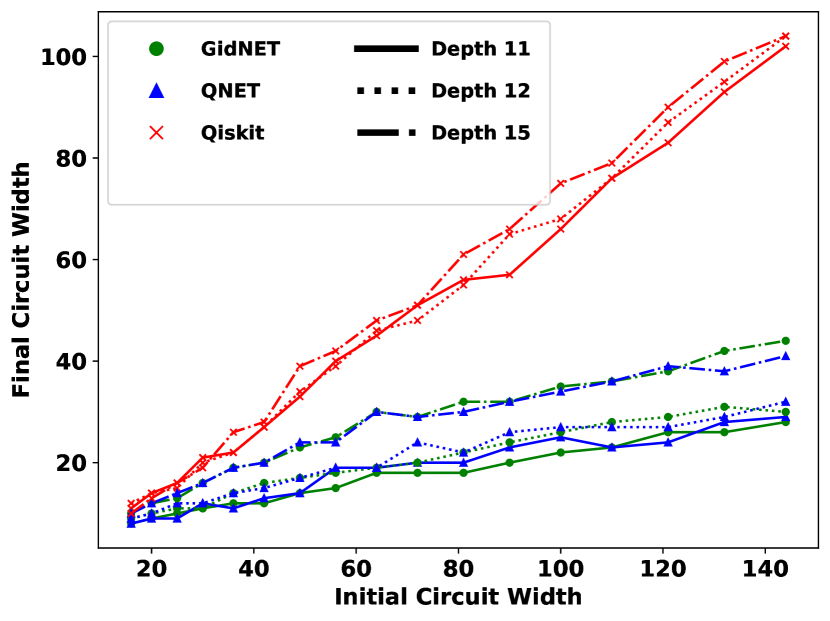
Figure 4: Comparison of the final circuit width achieved after qubit reuse compilation by GidNET, QNET, and Qiskit algorithms for GRCS circuits. GidNET performed better than the other algorithms in most cases.

To determine runtime performance, each circuit configuration was run a total of 7 times. The average runtime from these executions was then computed, and is shown in  Figure 5.

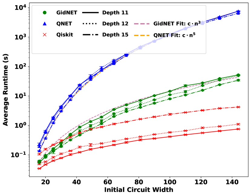
Figure 5: Comparison of GidNET, QNET, and Qiskit average runtimes for GRCS circuits.

Our study demonstrates that for GRCS circuits of depth 11, GidNET is faster by an average of 97.4% (or 38.5$\times$) reaching up to 99.3% (or 142.9$\times$) for circuit size 144 compared to QNET. This result shows GidNET’s superior ability to optimize quantum circuits, evidencing not only reduced circuit width but also enhanced runtime performance. Although Qiskit is on average 92.1% (or 12.7$\times$) faster in runtime, the significant improvement in circuit width (59.3%) by GidNET can be considered an acceptable tradeoff. For GRCS circuits of depths 12 and 15, GidNET is on average 46.9$\times$ and 48.7$\times$ faster than QNET respectively. Although Qiskit is 7.3$\times$ and 1.7$\times$ faster for GRCS circuits of depths 12 and 15 respectively, GidNET achieved a much better average width reduction (53.6% and 40.0%, respectively).

V-B Quantum Approximate Optimization Algorithm (QAOA)

The second benchmark set comprised the Quantum Approximate Optimization Algorithm (QAOA)  [36, 2, 1], which is designed for solving combinatorial optimization problems on quantum computers. The algorithm operates by applying a unitary transformation $U(\vec{\beta},\vec{\gamma})$, structured as a product of alternating operators, which are iteratively optimized to minimize the cost function encoded in the quantum circuit. The core of the QAOA is formed by repeatedly applying two types of unitary transformations for a total of $p$ layers, where $p$ influences solution quality and computational complexity:

$$U(\vec{\beta},\vec{\gamma})=\prod_{n=1}^{p}U_{B}(\beta_{n})U_{C}(\gamma_{n}).$$ (10)

Here, $U_{B}(\beta_{n})=e^{-i\beta_{n}H_{B}}$ and $H_{B}=\sum_{i}X_{i}$ is the mixing Hamiltonian, and $U_{C}(\gamma_{n})=e^{-i\gamma_{n}H_{C}}$ encodes the problem’s cost Hamiltonian. We used that of MaxCut,

$$H_{C}=\frac{1}{2}\sum_{(i,j)\in E}(1-z_{i}z_{j}).$$ (11)

We explored the runtime efficiency, and solution quality (with respect to the final or compressed circuit width) of applying the three algorithms to QAOA MaxCut problems on random unweighted three-regular (U3R) graphs. An U3R graph is a type of graph in which each vertex is connected to exactly three other vertices   [37]. The structural simplicity of U3R graphs, where the number of quantum gates mirrors the number of edges and scales linearly with the number of vertices, makes it a standard benchmark for QAOA on current hardware  [38, 39, 40]. Their shallow, broad layout, coupled with sparse gate connectivity, position MaxCut QAOA circuits as an ideal testbed for qubit reuse strategies.

Each algorithm was tested on QAOA circuits for two depths, $p=1$ ( Figure 6 and  Figure 7) and $p=2$ ( Figure 8 and  Figure 9), to evaluate how depth affects compression and performance for varying number of qubits. For each fixed number of qubits, 20 random U3R graphs were generated using the NetworkX package  [41]. The same set of random graphs were utilized to construct QAOA circuits for each of the three competing qubit reuse algorithms. Both GidNET and QNET algorithms were run 10 times for each circuit generated from each random graph, and the best result was recorded.

Figure 6 shows the boxplot comparing the circuit widths achieved by GidNET, QNET, and Qiskit for various circuit sizes. The range of widths, indicated by the vertical span of the boxes and whiskers, provides insight into the spread and median values of the circuit widths for each qubit reuse framework’s performance for different circuit sizes. Outliers are shown as individual points beyond the whiskers. The presence of outliers can indicate specific instances where a framework handles certain circuits unusually well (or poorly).

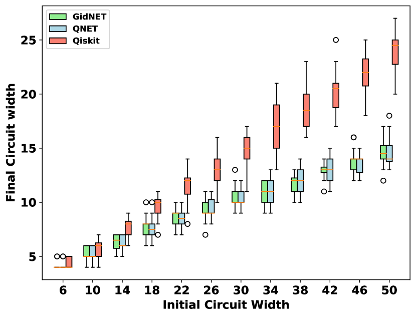
Figure 6: Comparison of final circuit widths achieved after qubit reuse compilation by GidNET, QNET, and Qiskit for QAOA circuits, $p=1$.

GidNET and QNET show similar performance in terms of circuit width across most sizes, with tightly grouped medians that are generally lower than those of Qiskit. Qiskit tends to have a wider spread and higher median values, particularly for larger circuit sizes. The presence of more outliers in Qiskit’s data could suggest that it is either particularly sensitive to certain circuit configurations or it might exploit specific configurations more effectively than others.

To determine the algorithmic runtime, each QAOA circuit generated from the U3R graph configuration was evaluated seven times. The average runtime across evaluations was computed to provide a consistent measure of performance.

In evaluating the complexity of the three qubit reuse algorithms across various QAOA circuit sizes for $p=1$, GidNET demonstrated significant performance superiority when compared to QNET and Qiskit as shown in  Figure 7. Our analysis showed that on average, GidNET operates approximately 87.9% (or 8.3$\times$) faster than QNET and 98.1% (or 52.6$\times$) faster than Qiskit. This substantial speed advantage highlights GidNET’s ability in managing qubit resources, positioning it as a highly effective tool for qubit reuse.

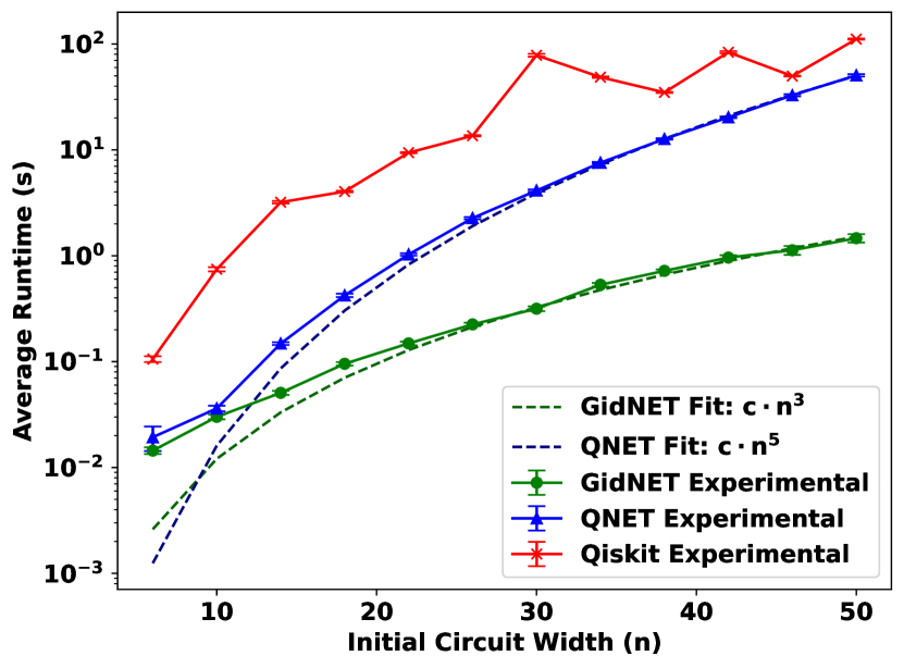
Figure 7: Comparison of GidNET, QNET and Qiskit Average Runtime for QAOA Circuit, $p$=1.

Figure 8 compares the performance of GidNET and QNET qubit reuse algorithms on QAOA circuits with $p=2$. Both algorithms demonstrated similar effectiveness across circuit sizes, with GidNET showing a marginal advantage in achieving slightly smaller widths, especially as circuit complexity increased. Our result shows that on average, GidNET achieved 1.4% improvement in circuit width reduction reaching up to 3.4% for circuit size 42 over QNET. The variability in widths also grew with circuit size for both algorithms. We excluded the Qiskit qubit reuse algorithm from this analysis as its longer runtime made it impractical especially for larger circuits.

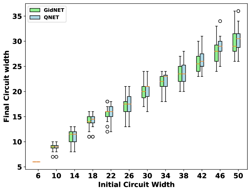
Figure 8: Comparison of final circuit widths after qubit reuse compilation by GidNET and QNET for QAOA circuits, $p$=2.

Figure 9 compares the runtimes of GidNET and QNET for QAOA circuits with $p=2$. The analysis reveals that GidNET generally demonstrates better runtime, particularly as the circuit size increases. GidNET shows an average runtime improvement of 82.9% (5.8$\times$) over QNET. This performance becomes more pronounced for larger circuits: for 50-qubit circuits, we observe a runtime improvement of about 97.4% (38.5$\times$). This pattern indicates that GidNET is particularly effective in managing the increased complexity of larger circuits, making it a potentially more suitable choice for extensive qubit reuse tasks where runtime is critical.

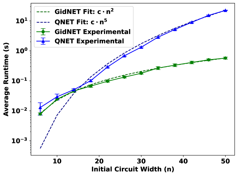
Figure 9: Comparison of GidNET and QNET Average Runtime for QAOA Circuit, $p$=2 (average over 7 runs of 1 graph).

V-C Statistical Validation of Complexity Analysis

Statistical analysis via polynomial regression was employed to evaluate how well the theoretically obtained complexity analyses of GidNET and QNET align with experimental results. This approach involved fitting polynomial models to the runtime data, with each model’s coefficients tested to ascertain their impact. The primary objective was to validate the theoretical predictions against actual performance as circuit complexity increased. The selected degrees of the polynomials were based on reported computational complexities. QNET’s complexity was previously established as $O(mn+n^{5})$  [1], prompting our choice of a fifth-degree polynomial ($n^{5}$) for its analysis. Similarly, GidNET, with a reported complexity of $O(mn^{2}+\mu\nu k^{2}+pn^{3}\log{n})$, was analyzed using a third-degree polynomial ($n^{3}$).

F-tests and R-squared values were employed to assess the models across various circuits. The results are summarized in  Table I. To avoid cluttering  Figure 5, we show only the polynomial fit for depth 11 GRCS circuits for GidNET and QNET. The F-statistics were $2874.84$ for GidNET and $3725.56$ for QNET, indicating strong model fits, with R-squared values at $0.9990$ and $0.9996$ respectively, demonstrating that nearly all variance in the experimental data was accounted for.

In the case of QAOA circuits with $p=1$, GidNET’s F-statistic was $614.2$, and QNET’s was $19968.28$, with corresponding R-squared values of $0.9999$ and $0.99996$, indicating that both models provide a highly adequate fit to the reported complexities. For QAOA circuits with $p=2$, GidNET was fitted with polynomial $n^{2}$. This is because, although polynomial $n^{3}$ and $n^{2}$ have approximately the same R-squared value of $0.998$, $n^{3}$ with F-statistic of $800.95$ shows a worse fit compared to $n^{2}$ with F-statistic of $1117.60$. Also, depending on the circuit structure, it is common that not all the GidNET iterations are needed to achieve optimal reuse. QNET maintained a strong model fit with an F-statistic of $1925.77$ and an R-squared value of $0.9996$. These results not only substantiate the regression models’ fit but also reinforce the credibility of the statistical validation by directly tying it to the theoretical framework of each algorithm.

TABLE I: Statistical Analysis Results for GidNET and QNET on Various Circuits

Algorithm	Circuit	R-squared Value	F-statistic
GidNET	GRCS Circuit ($d=11$)	0.9990	2874.84
QNET	GRCS Circuit ($d=11$)	0.9996	3725.56
GidNET	QAOA Circuit ($p=1$)	0.9971	614.2
QNET	QAOA Circuit ($p=1$)	1.0000	19968.28
GidNET	QAOA Circuit ($p=2$)	0.9976	1117.60
QNET	QAOA Circuit ($p=2$)	0.9996	1925.77

We suspect the variations in the fit of polynomial models for QAOA and GRCS circuits can be attributed to the difference in circuit sizes used in the experiments. Specifically, QAOA circuits were tested with a smaller number of qubits compared to the GRCS circuits. The accuracy of the polynomial models tends to improve for circuits with more qubits.

VI Conclusion and Future Work

This paper introduces GidNET (Graph-based Identification of qubit NETwork), a novel algorithm aimed at optimizing qubit reuse in quantum circuits to manage quantum resource constraints in current architectures. By leveraging the circuit’s DAG and candidate matrix, GidNET efficiently identifies pathways for qubit reuse to reduce quantum resource requirements.

The core advantage of GidNET over other algorithms lies in its ability to offer improved solutions with more scalable computational demands. Our comparative analysis with existing algorithms, particularly QNET, shows that GidNET not only achieves smaller compiled circuit widths by an average of 4.4%, with reductions reaching up to 21% for larger circuits, but speeds up computations, achieving significant runtime improvements by an average of 97.4% (or 38.5$\times$) reaching up to 99.3% (or 142.9$\times$) across varying circuit sizes. This makes GidNET a highly effective choice for larger and more complex quantum circuits where both compilation time and qubit management are crucial factors. These results underscore the critical role of advanced qubit reuse strategies in optimizing quantum computations, providing a robust solution that bridges the gap between exact algorithmic precision and heuristic scalability, and a valuable benchmark for further development in this field.

GidNET, while offering advancements in qubit reuse optimization for quantum circuits, is not without limitations. For example, the performance of GidNET could vary across different quantum hardware architectures, requiring specific tailoring to individual systems. Hence, future enhancements to GidNET could involve adapting it for specific quantum hardware architectures, and expanding its scope to multi-objective optimizations that consider not only circuit width but also depth and gate count. Additionally, integrating machine learning techniques could refine its graph-based strategies, potentially offering more dynamic and optimized qubit reuse sequences. A better method for updating the candidate matrix could result in improved complexity of GidNET making it possible to use GidNET for industry grade circuits requiring large number of qubits. These advancements could make GidNET a more versatile and powerful tool in optimizing quantum circuits for practical quantum computing applications.

References

- [1] K. Fang, M. Zhang, R. Shi, and Y. Li, “Dynamic quantum circuit compilation,” arXiv preprint arXiv:2310.11021, 2023.
- [2] M. DeCross, E. Chertkov, M. Kohagen, and M. Foss-Feig, “Qubit-reuse compilation with mid-circuit measurement and reset,” Physical Review X, vol. 13, no. 4, p. 041057, 2023.
- [3] M. Sadeghi, S. Khadirsharbiyani, and M. T. Kandemir, “Quantum circuit resizing,” arXiv preprint arXiv:2301.00720, 2022.
- [4] J. M. Pino, J. M. Dreiling, C. Figgatt, J. P. Gaebler, S. A. Moses, M. Allman, C. Baldwin, M. Foss-Feig, D. Hayes, K. Mayer et al., “Demonstration of the trapped-ion quantum ccd computer architecture,” Nature, vol. 592, no. 7853, pp. 209–213, 2021.
- [5] IBM, “Quantum dynamic circuits,” 2023, online; accessed 2023-04-10. [Online]. Available: https://www.ibm.com/quantum/blog/quantum-dynamic-circuits
- [6] A. D. Córcoles, M. Takita, K. Inoue, S. Lekuch, Z. K. Minev, J. M. Chow, and J. M. Gambetta, “Exploiting dynamic quantum circuits in a quantum algorithm with superconducting qubits,” Physical Review Letters, vol. 127, no. 10, p. 100501, 2021.
- [7] C. Ryan-Anderson, N. Brown, M. Allman, B. Arkin, G. Asa-Attuah, C. Baldwin, J. Berg, J. Bohnet, S. Braxton, N. Burdick et al., “Implementing fault-tolerant entangling gates on the five-qubit code and the color code,” arXiv preprint arXiv:2208.01863, 2022.
- [8] E. Chertkov, J. Bohnet, D. Francois, J. Gaebler, D. Gresh, A. Hankin, K. Lee, D. Hayes, B. Neyenhuis, R. Stutz et al., “Holographic dynamics simulations with a trapped-ion quantum computer,” Nature Physics, vol. 18, no. 9, pp. 1074–1079, 2022.
- [9] J. Yirka and Y. Subaşı, “Qubit-efficient entanglement spectroscopy using qubit resets,” Quantum, vol. 5, p. 535, 2021.
- [10] C. Harvey, R. Yeung, and K. Meichanetzidis, “Sequence processing with quantum tensor networks,” arXiv preprint arXiv:2308.07865, 2023.
- [11] S. Brandhofer, I. Polian, and K. Krsulich, “Optimal qubit reuse for near-term quantum computers,” in 2023 IEEE International Conference on Quantum Computing and Engineering (QCE), vol. 1. IEEE, 2023, pp. 859–869.
- [12] F. Hua, Y. Jin, Y. Chen, S. Vittal, K. Krsulich, L. S. Bishop, J. Lapeyre, A. Javadi-Abhari, and E. Z. Zhang, “Exploiting qubit reuse through mid-circuit measurement and reset,” arXiv preprint arXiv:2211.01925, 2022.
- [13] T. Peng, A. Harrow, M. Ozols, and X. Wu, “Simulating large quantum circuits on a small quantum computer,” Physical Review Letters, vol. 125, p. 150504, 2020.
- [14] G. Uchehara, T. M. Aamodt, and O. Di Matteo, “Rotation-inspired circuit cut optimization,” in 2022 IEEE/ACM Third International Workshop on Quantum Computing Software (QCS). IEEE, 2022, pp. 50–56.
- [15] M. A. Perlin, Z. H. Saleem, M. Suchara, and J. C. Osborn, “Quantum circuit cutting with maximum-likelihood tomography,” npj Quantum Information, vol. 7, no. 1, p. 1–11, 2021.
- [16] W. Tang, T. Tomesh, M. Suchara, J. Larson, and M. Martonosi, “Cutqc: using small quantum computers for large quantum circuit evaluations,” in Proceedings of the 26th ACM International conference on architectural support for programming languages and operating systems, 2021, pp. 473–486.
- [17] A. Lowe, M. Medvidović, A. Hayes, L. J. O’Riordan, T. R. Bromley, J. M. Arrazola, and N. Killoran, “Fast quantum circuit cutting with randomized measurements,” Quantum, vol. 7, p. 934, 2022.
- [18] L. Brenner, C. Piveteau, and D. Sutter, “Optimal wire cutting with classical communication,” arXiv preprint arXiv:2302.03366, 2023.
- [19] H. Harada, K. Wada, and N. Yamamoto, “Optimal parallel wire cutting without ancilla qubits,” arXiv preprint arXiv:2303.07340, 2023.
- [20] C. Piveteau and D. Sutter, “Circuit knitting with classical communication,” arXiv preprint arXiv:2205.00016, 2022.
- [21] K. Mitarai and K. Fujii, “Overhead for simulating a non-local channel with local channels by quasiprobability sampling,” Quantum, vol. 5, p. 388, 2021.
- [22] C. Ufrecht, M. Periyasamy, S. Rietsch, D. D. Scherer, A. Plinge, and C. Mutschler, “Cutting multi-control quantum gates with zx calculus,” arXiv preprint arXiv:2302.00387, 2023.
- [23] K. Mitarai and K. Fujii, “Constructing a virtual two-qubit gate by sampling single-qubit operations,” New Journal of Physics, vol. 23, no. 2, p. 023021, 2021.
- [24] S. Brandhofer, I. Polian, and K. Krsulich, “Optimal partitioning of quantum circuits using gate cuts and wire cuts,” IEEE Transactions on Quantum Engineering, 2023.
- [25] O. Di Matteo, M. A. Perlin, Z. H. Saleem, M. Suchara, and J. C. Osborn, “Quantum-circuit cutting fills a gaping quantum computing hole,” Communications of the ACM, vol. 65, no. 1, p. 18–20, 2022.
- [26] F. Hua, Y. Jin, Y. Chen, S. Vittal, K. Krsulich, L. S. Bishop, J. Lapeyre, A. Javadi-Abhari, and E. Z. Zhang, “Caqr: A compiler-assisted approach for qubit reuse through dynamic circuit,” in Proceedings of the 28th ACM International Conference on Architectural Support for Programming Languages and Operating Systems, Volume 3, 2023, pp. 59–71.
- [27] A. Pawar, Y. Li, Z. Mo, Y. Guo, Y. Zhang, X. Tang, and J. Yang, “Integrated qubit reuse and circuit cutting for large quantum circuit evaluation,” arXiv preprint arXiv:2312.10298, 2023.
- [28] S. Niu, A. Hashim, C. Iancu, W. A. de Jong, and E. Younis, “Powerful quantum circuit resizing with resource efficient synthesis,” arXiv preprint arXiv:2311.13107, 2023.
- [29] S. Brandhofer, I. Polian, and K. Krsulich, “Optimal qubit reuse for near-term quantum computers,” in 2023 IEEE International Conference on Quantum Computing and Engineering (QCE), vol. 1. IEEE, 2023, pp. 859–869.
- [30] P. W. Shor, “Algorithms for quantum computation: discrete logarithms and factoring,” in Proceedings 35th annual symposium on foundations of computer science. Ieee, 1994, pp. 124–134.
- [31] L. K. Grover, “A fast quantum mechanical algorithm for database search,” in Proceedings of the twenty-eighth annual ACM symposium on Theory of computing, 1996, pp. 212–219.
- [32] J. Biamonte, P. Wittek, N. Pancotti, P. Rebentrost, N. Wiebe, and S. Lloyd, “Quantum machine learning,” Nature, vol. 549, no. 7671, pp. 195–202, 2017.
- [33] A. Paler, R. Wille, and S. J. Devitt, “Wire recycling for quantum circuit optimization,” Physical Review A, vol. 94, no. 4, p. 042337, 2016.
- [34] Q. Community, “Qiskit qubit reuse,” https://github.com/qiskit-community/qiskit-qubit-reuse, 2023, gitHub repository.
- [35] S. Boixo, S. V. Isakov, V. N. Smelyanskiy, R. Babbush, N. Ding, Z. Jiang, M. J. Bremner, J. M. Martinis, and H. Neven, “Characterizing quantum supremacy in near-term devices,” Nature Physics, vol. 14, no. 6, pp. 595–600, 2018.
- [36] E. Farhi, J. Goldstone, and S. Gutmann, “A quantum approximate optimization algorithm,” arXiv preprint arXiv:1411.4028, 2014.
- [37] Y. Chai, Y.-J. Han, Y.-C. Wu, Y. Li, M. Dou, and G.-P. Guo, “Shortcuts to the quantum approximate optimization algorithm,” Physical Review A, vol. 105, no. 4, p. 042415, 2022.
- [38] L. Zhou, S.-T. Wang, S. Choi, H. Pichler, and M. D. Lukin, “Quantum approximate optimization algorithm: Performance, mechanism, and implementation on near-term devices,” Physical Review X, vol. 10, no. 2, p. 021067, 2020.
- [39] M. P. Harrigan, K. J. Sung, M. Neeley, K. J. Satzinger, F. Arute, K. Arya, J. Atalaya, J. C. Bardin, R. Barends, S. Boixo et al., “Quantum approximate optimization of non-planar graph problems on a planar superconducting processor,” Nature Physics, vol. 17, no. 3, pp. 332–336, 2021.
- [40] S. Ebadi, A. Keesling, M. Cain, T. T. Wang, H. Levine, D. Bluvstein, G. Semeghini, A. Omran, J.-G. Liu, R. Samajdar et al., “Quantum optimization of maximum independent set using rydberg atom arrays,” Science, vol. 376, no. 6598, pp. 1209–1215, 2022.
- [41] A. Hagberg, P. Swart, and D. S Chult, “Exploring network structure, dynamics, and function using networkx,” Los Alamos National Lab.(LANL), Los Alamos, NM (United States), Tech. Rep., 2008.