Uncertainty-Aware Optimal Treatment Selection
for Clinical Time Series

Abstract

In personalized medicine, the ability to predict and optimize treatment outcomes across various time frames is essential. Additionally, the ability to select cost-effective treatments within specific budget constraints is critical. Despite recent advancements in estimating counterfactual trajectories, a direct link to optimal treatment selection based on these estimates is missing. This paper introduces a novel method integrating counterfactual estimation techniques and uncertainty quantification to recommend personalized treatment plans adhering to predefined cost constraints. Our approach is distinctive in its handling of continuous treatment variables and its incorporation of uncertainty quantification to improve prediction reliability. We validate our method using two simulated datasets, one focused on the cardiovascular system and the other on COVID-19. Our findings indicate that our method has robust performance across different counterfactual estimation baselines, showing that introducing uncertainty quantification in these settings helps the current baselines in finding more reliable and accurate treatment selection. The robustness of our method across various settings highlights its potential for broad applicability in personalized healthcare solutions.

1 Introduction

In recent years, there has been a growing interest within medical research in forecasting patient data across various time periods and predicting future treatment effects, a trend that aligns well with the longitudinal nature of healthcare data (Allam et al., 2021; Liu et al., 2023; Feuerriegel et al., 2024). This is particularly important in personalized medicine, where the goal is usually to develop treatment plans that are tailored to the predicted health development of individual patients (Moodie et al., 2007; van Geloven et al., 2020). A critical aspect of these plans is the reliability of the predictions (Utomo et al., 2018; Hess et al., 2023), as practitioners often prefer more certain outcomes over those that are merely optimistic or cost-effective (Kerr et al., 2008; West and West, 2002). Additionally, the cost and potential side effects of treatments must be considered, particularly for high-dose treatments (Weiting et al., 2022; Auger et al., 2005; Frei III and Canellos, 1980).

While several studies have explored counterfactual estimations and uncertainty quantification in longitudinal data (Bica et al., 2020a; Hess et al., 2023; Li et al., 2021; Brouwer et al., 2022), there remains a gap in applying these techniques to inform treatment assignment strategies. Notably, existing strategies often overlook the continuous nature of many treatment decisions, such as chemotherapy dosing (Kallus and Zhou, 2018; Kreif et al., 2015).

Contributions.

This work introduces a model-agnostic framework for optimal treatment selection that integrates uncertainty quantification of counterfactual predictions within predefined cost constraints. Our approach effectively accommodates continuous-valued treatments and is compatible with various uncertainty quantification and counterfactual prediction methodologies, enhancing its applicability across different settings.

2 Related Work

Treatment effect trajectories estimation.

In the realm of longitudinal data, recent years have seen various developments in estimating treatment effects, with a focus on the trajectories of individual patients. Bica et al. (2020a) introduced a counterfactual recurrent neural network (CRN) that utilizes an encoder-decoder style long-short-term memory network. Following this, Melnychuk et al. (2022) incorporated the transformer architecture to create the causal transformer (CT), and Seedat et al. (2022) addressed irregularly sampled time series by employing neural controlled differential equations (TE-CDE). Counterfactual ODE (CF-ODE) (Brouwer et al., 2022) and Bayesian neural controlled differential equation BNCDE (Hess et al., 2023) later followed, including uncertainty quantification into counterfactual trajectories estimation. Recent models for counterfactual predictions based on g-computations were also introduced, like G-NET (Li et al., 2021). However, these studies primarily concentrate on scenarios involving treatments with discrete values, such as fixed dosages per treatment type.

Balancing representations.

Prior works have concentrated on estimating counterfactual trajectories with temporal confounding, where past covariates influence both the outcome and the treatment. To counteract treatment selection bias in time series models, Bica et al. (2020a), Seedat et al. (2022) and Melnychuk et al. (2022) have explored the development of a treatment-invariant representation through domain adversarial losses. Liu et al. (2023) implemented propensity score matching in mini-batches as a strategy to mitigate temporal confounding. These methods typically assume treatments with discrete values. However, the efficacy of balancing representations in addressing these issues has recently received attention. Such approaches might only be beneficial in certain conditions, such as with small sample sizes, as suggested by Alaa and Schaar (2018), or involving numerous noisy covariates, as noted by Johansson et al. (2022). Hess et al. (2023) have highlighted that balancing representations might not effectively reduce bias in scenarios with time-varying confounders due to identifiability challenges. Similarly, our supplementary experiments do not support balancing representations as means to address temporal confounding, see Appendix B. Additionally, even in static contexts, these representations face complications due to the invertibility assumption imposed on the learned representations (Shalit et al., 2017). For a more comprehensive analysis, we refer the reader to Melnychuk et al. (2023) and Curth and van der Schaar (2021).

Uncertainty quantification in treatment effect estimation.

Various studies have incorporated uncertainty quantification in treatment effect estimations over time. TE-CDE (Seedat et al., 2022) and G-NET (Li et al., 2021) use Monte Carlo (MC) dropout (Gal and Ghahramani, 2016) to approximate the posterior distributions of counterfactual outcomes. However, Hess et al. (2023) note that MC dropout provides poor approximation of a posterior, proposing instead a Bayesian deep learning approach in BNCDE that operates in continuous time. Their findings suggest that deferring treatments with high uncertainty can significantly lower the error in outcome prediction. However, this method only accounts for uncertainty quantification of predictions of single time steps (instead of multiple time steps) and, like previous approaches, is limited to discrete treatments. CF-ODE puts further attention on uncertainty quantification, as it helps in detecting a lack of overlap between treated and non-treated distributions and confounding issues (Brouwer et al., 2022).

Optimal treatment selection.

Optimal treatment strategy for healthcare, with the goal of maximising clinical outcomes, has been extensively studied (Caye et al., 2019; Dienstmann et al., 2015; Zhang et al., 2012; Murphy, 2003; Robins et al., 2004; Moodie et al., 2007). Different approaches have been studied, including variable selection (Lu et al., 2013; Song et al., 2015), multicriteria decision-making methods with conflicting outcomes (Bellos, 2023), optimal treatments selection based on predictive factors (Polley and van der Laan, 2009), multiple treatments assignment (Lou et al., 2018). To the best of our knowledge, previous optimal treatments selection frameworks have not, however, been linked with uncertainty-aware counterfactual estimation in longitudinal data.

3 Model and Problem Setting

Problem setting.

We consider longitudinal datasets, each consisting of $n$ multidimensional patient trajectories. Each trajectory includes: the outcomes ($\mathbf{Y}_{t}\in\mathbb{R}^{d_{y}}$), the treatments ($\mathbf{A}_{t}\in\mathbb{R}^{d_{a}}$), the observed covariates ($\mathbf{X}_{t}\in\mathbb{R}^{d_{x}}$). We denote the history of all observed covariates up to time $t$ for patient $i\in\{1,\ldots,n\}$ as $\bar{\mathbf{H}}_{t}^{i}=\{\bar{\mathbf{X}}_{t}^{i},\bar{\mathbf{A}}_{t}^{i},\bar{\mathbf{Y}}_{t}^{i}\}$, with $\bar{\mathbf{X}}_{t}^{i}:=\mathbf{X}^{i}_{[0,t]}$. In the following, we omit the $i$ for better readability. This notation follows from (Melnychuk et al., 2022; Bica et al., 2020a).

We use the potential outcomes frameworks (Rubin, 2005), extended to accommodate time-varying treatments (Robins et al., 2004). Our observational period spans $[0,t]$, and we consider future projections over a time horizon $\tau\geq 0$, within the interval $[t,t+\tau]$. Given a continuous-valued intervention on the treatment ${\mathbf{a}}_{t:t+\tau}=\mathbf{a}_{[t,t+\tau]}$, we are interested in the values of ${\mathbf{Y}}_{t:t+\tau}[{\mathbf{a}}_{t:t+\tau}]$, which represents the potential outcome $\mathbf{Y}$ over the interval $[t,t+\tau]$ following an intervention on ${\mathbf{A}}_{t:t+\tau}$. Generally, works like Bica et al. (2020a) are interested in the point estimate $\mathbb{E}[{\mathbf{Y}}_{t:t+\tau}[{\mathbf{a}}_{t:t+\tau}]\mid\bar{\mathbf{h}}_{t}]$, corresponding to the future counterfactual outcomes ${\mathbf{Y}}_{t:t+\tau}$ following an intervention ${\mathbf{a}}_{t:t+\tau}$, on a patient with history $\bar{\mathbf{h}}_{t}$. We make the standard assumptions needed for the identification of potential outcomes from observational data: consistency, sequential ignorability, and sequential overlap (Lim, 2018; Robins et al., 2004).

Similarly to Hess et al. (2023); Brouwer et al. (2022), our goal is to estimate uncertainty-aware counterfactual trajectories to aid in selecting reliable treatment strategies. Given a desired outcome trajectory ${\mathbf{y}}^{*}_{t:t+\tau}$, we would like to select the optimal treatment trajectory ${\mathbf{a}}^{*}_{t:t+\tau}$ such that

$$\min_{{\mathbf{a}}_{t:t+\tau}\in S({\mathbf{A}}_{t:t+\tau})}\{\|\mathbb{E}[{\mathbf{Y}}_{t:t+\tau}[{\mathbf{a}}_{t:t+\tau}]\mid\bar{\mathbf{h}}_{t}]-{\mathbf{y}}^{*}_{t:t+\tau}\|^{2}+\lambda\text{Var}[{\mathbf{Y}}_{t:t+\tau}[{\mathbf{a}}_{t:t+\tau}]\mid\bar{\mathbf{h}}_{t}]]\}\>,$$

where $\lambda$ is the uncertainty weight. Here, $S(\mathbf{A}_{t:t+\tau})\subseteq\mathcal{A}$ with $\mathbf{A}_{t:t+\tau}\in\mathcal{A}$ represents the outcome trajectories satisfying a defined constraint.

Uncertainty quantification and treatment selection.

We select as counterfactual trajectories estimation methods the baselines: CF-ODE, BNCDE, G-NET, CRN, CT. We will refer to these counterfactual estimation neural network-based models ${G}_{\phi_{t}}:\mathbb{R}^{d_{a}+d_{x}+d_{v}}\rightarrow\mathbb{R}^{d_{y}}$, estimating $\mathbb{E}[{\mathbf{Y}}_{t^{\prime}}[{\mathbf{a}}_{t:t+\tau}]\mid\bar{\mathbf{h}}_{t}]$ from ${\mathbf{a}}_{t:t+\tau}$ and $\bar{\mathbf{h}}_{t}$ with $t^{\prime}\in[t,t+\tau]$. More details on the uncertainty estimation and implementation of models can be found in Appendix A.

To assess the uncertainty of counterfactual predictions, we employ three model-agnostic techniques: Monte-Carlo (MC) dropout, ensembling, and geometric ensembling, as discussed by Garipov et al. (2018). For MC-dropout, we perform eight forward passes, calculating the average $\hat{\mathbf{\mathbf{\mu}}}_{t:t+\tau}({\mathbf{a}}_{t},\bar{\mathbf{h}}_{t})$ and variance $\hat{\mathbf{\sigma}}_{t:t+\tau}({\mathbf{a}}_{t},\bar{\mathbf{h}}_{t})$ of the predicted counterfactual outcomes $\hat{\mathbf{y}}_{t:t+\tau}={G}_{\phi_{t}}({\mathbf{a}}_{t:t+\tau},\bar{\mathbf{h}}_{t:t+\tau})$. Similarly, in the ensembling approach, we utilize a group of eight models to compute these statistics. Geometric ensembling, chosen for its training and computation efficiency, also involves sampling eight neural networks to determine the average and variance of predictions. MC-dropout, due to its superior speed, is our primary method for most treatment selection experiments. Additionally, for models incorporating neural stochastic differential equations (BNCDE and CF-ODE), we conduct eight forward passes to compute both the average and variance of the counterfactual outcome predictions, ensuring consistency in our experimental approach. We perform treatment selection with the following objective

$$\min_{\bar{\mathbf{a}}_{t:t+\tau}\in S({\mathbf{A}}_{t:t+\tau})}\{\frac{1}{\tau}\sum_{i=1}^{\tau}(\hat{\mathbf{\mathbf{\mu}}}_{t+i}({\mathbf{a}}_{t+i},\bar{\mathbf{h}}_{t+i})-\mathbf{y}_{t+i})^{2}+\lambda\frac{1}{\tau}\sum_{i=1}^{\tau}\hat{\mathbf{\sigma}}_{t+i}({\mathbf{a}}_{t+i},\bar{\mathbf{h}}_{t+i})^{2}\}\>.$$

More information on the choice of the treatment constraint $S({\mathbf{A}}_{t:t+\tau})$ can be found in Section D.1.We utilize gradients available through auto-differentiation to perform gradient descent on the loss function using the AdamW optimizer (Loshchilov and Hutter, 2019).

Evaluation.

To evaluate how reliably the selected treatments achieve the desired outcomes, we leverage the ground truth dynamics from which the data is simulated. We simulate the counterfactual trajectory ${\mathbf{Y}}_{t:t+\tau}({\mathbf{a}}^{*}_{t:t+\tau})$ for the selected treatment $\mathbf{a}^{*}_{t:t+\tau}$ and compare it with the counterfactual estimation ${G}_{\phi_{t}}({\mathbf{a}}^{*}_{t:t+\tau},\bar{\mathbf{h}}_{t})$. We evaluate the reliability of the treatment selection as the root mean squared error between the counterfactual outcome and the desired outcome ${\mathbf{Y}}_{t:t+\tau}({\mathbf{a}}^{*}_{t:t+\tau})$

$$\text{RMSE}_{\text{selection}}=\sqrt{\frac{1}{\tau}\sum_{i=1}^{\tau}(\hat{\mathbf{\mathbf{\mu}}}_{t+i}({\mathbf{a}}^{*}_{t+i},\bar{\mathbf{h}}_{t+i})-\bar{\mathbf{Y}}_{t+i}({\mathbf{a}}^{*}_{t+i}))^{2}}\>.$$

4 Experiments

We evaluate our model using different counterfactual estimation baselines, uncertainty quantification methods and treatment constraints on two simulated datasets. More details on the parameters used can be found in Section D.2.

4.1 Data

We utilize two simulated medical datasets focused on the COVID-19 and cardiovascular system to evaluate our model. The use of simulated data is essential as it provides access to true counterfactual trajectories, which are crucial for assessing our method’s performance. For all datasets, we simulate 40 time steps of observations in the interval $[0,30]$ ($t=30$) and consider a prediction window of $[30,40]$, with $\tau=10$. We generate $\bar{\mathbf{H}}_{t+\tau}$ for each patient from randomly sampled initial conditions. We use 1024, 128, and 128 patients as training, validation and test set, respectively.

COVID-19 dataset.

We use the synthetic dataset by (Qian et al., 2021), which is an extension of the one proposed in Dai et al. (2021) following

$$\dot{Z}_{1}(t) =k_{dp}Z_{1}(t)-k_{di}Z_{1}(t)Z_{3}(t)-k_{dr}Z_{1}(t)Z_{2}(t)\>,$$

$$\dot{Z}_{2}(t) =k_{id}Z_{1}(t)-k_{io}Z_{2}(t)+k_{if}Z_{1}(t)Z_{2}(t)+\frac{k_{ep}Z_{2}^{h_{p}}}{k_{c_{p}}^{h_{p}}+Z_{2}^{h_{p}}}-k_{d}Z_{3}(t)Z_{2}(t)\>,$$

$$\dot{Z}_{3}(t) =k_{im}Z_{2}(t)\>,$$

$$\dot{Z}_{4}(t) =k_{kel}C(t)-k_{kel}Z_{3}(t)\>,$$

where $\dot{Z}_{i}(t)=\tfrac{dZ_{i}(t)}{dt}$ and $Z_{1}(t)$, $Z_{2}(t)$, $Z_{3}(t)$ , $Z_{4}(t)$ model the disease progression, immune reaction, immunity, and dose, respectively.

To model a clinical setting, we consider multiple treatment cycles, at the beginning of which a clinician can adjust the dose $\theta$ based on intermediate outcomes (5 cycles). Specifically, we consider that the treatment $Z_{4}(t)$ is increased by 10% every time the outcome $Z_{1}(t)$ increases from the previous time step, otherwise it is decreased by 10%.

Cardiovascular dataset.

We use the cardiovascular system (CVS) model proposed in Zenker et al. (2007), modelling the heart, the venous and arterial subsystems and the nervous system control of blood pressure in response to fluid intake. Specifically, we use the same underlying model as Brouwer et al. (2022); Linial et al. (2021)—a simplification of the one in Zenker et al. (2007)

$$\dot{SV}(t) =I_{\mathrm{external}}\>,$$

$$\dot{P}_{a}(t) =C_{a}^{-1}\Bigl{(}\frac{P_{a}(t)-P_{v}(t)}{R_{\mathrm{TPR}}(S)}-SV\cdot f_{\mathrm{HR}}(S)\Bigr{)}\>,$$

$$\dot{P}_{v}(t) =C_{v}^{-1}(-C_{a}\dot{P}_{a}(t)+I_{\mathrm{external}})\>,$$

$$\dot{S}(t) =\tau_{\mathrm{Baro}}^{-1}\Bigl{(}1-\frac{1}{1+\exp(-k_{\mathrm{width}}(P_{a}(t)-P_{a_{\mathrm{set}}})}-S\Bigr{)}\>,$$

with

$$R_{\mathrm{TPR}} =S(t)(R_{{\mathrm{TPR}}_{\max}}-R_{{\mathrm{TPR}}_{\min}})+R_{{\mathrm{TPR}}_{\min}}+R_{{\mathrm{TPR}}_{\mathrm{mod}}}\>,$$

$$f_{\mathrm{HR}}(S) =S(t)(f_{{\mathrm{HR}}_{\max}}-f_{{\mathrm{HR}}_{\min}})+f_{{\mathrm{HR}}_{\min}}\>,$$

$$I_{\mathrm{external}} =\theta\cdot e^{-\frac{5-t}{5}}\>.$$

Here, $SV$, $P_{a}$, $P_{v}$, $S$ represent the cardiac stroke volume, arterial blood pressure, venous blood pressure, and autonomic baroreflex tone, respectively, and $\theta$ represents the dosage. We consider the setting of a fluid challenge, in which fluid is administered to treat hypotension. In this setting, the outcome is the venous blood pressure $P_{v}$ and the treatment is a continuous-valued treatment process $I_{\text{external}}$( Brouwer et al. (2022)). We consider cycles of treatment, sampling a new continuous valued dose at the beginning of each cycle (5 cycles). More details on the parameters, and sampling the initial conditions as well as $\theta$ can be found in Appendix C.

4.2 Results

We evaluate the performance of our method using the cardiovascular and COVID-19 datasets, using different counterfactual estimators. Figure 1 shows how incorporating uncertainty quantification into the optimization objective overall increases the reliability of treatment selection for both datasets. However, in the cardiovascular dataset, certain baselines exhibit a local minimum within the tested range of uncertainty penalties. This phenomenon can be attributed to the dominance of the uncertainty penalty in the treatment selection objective. As the weights of uncertainty in the regularization term increase, the selected treatments deviate from achieving the desired outcomes, resulting in less accurate predictions and an increase in the root mean square error (RMSE). Differently, in the COVID-19 dataset, all the methods show increased performance among all selected uncertainty weights. In Figures 2 and 3, the performance of the method is shown to be robust among different treatment constraints and uncertainty metrics respectively using the CRN counterfactual estimation. More details on the clamping approaches can be found in Section D.1.

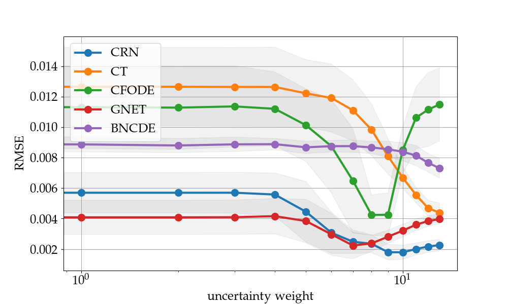
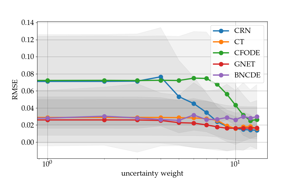
Figure 1: Performance of the baselines CRN, CT, CF-ODE, G-NET, BNCDE when selecting treatments for patients from the cardiovascular (left) and COVID-19 (right) datasets. For most baselines, the $\text{RMSE}_{\text{selection}}$ for the potential outcome compared to the desired outcome decreases, the higher the uncertainty weight in the optimization.

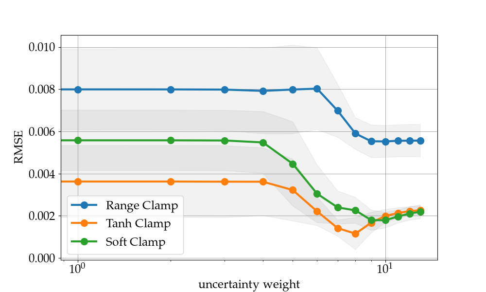
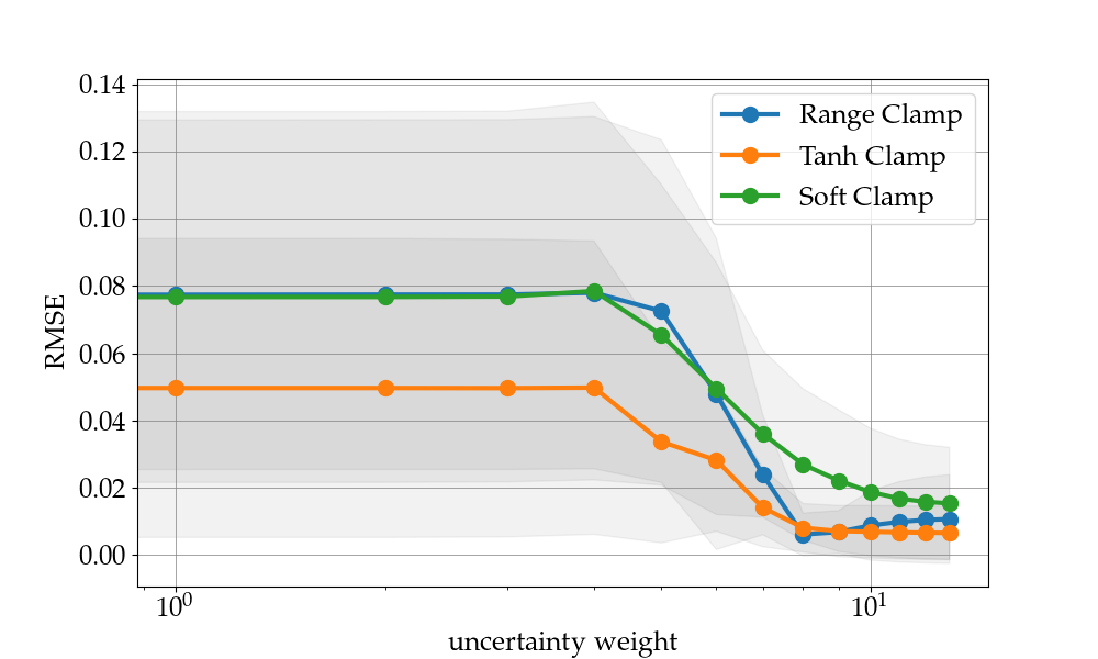
Figure 2: Comparison of clamping constraints for treatment selection, using the CRN as a counterfactual estimator under a range of uncertainty weights. On the left we show results on the cardiovascular dataset and on the right on the COVID-19 dataset. The performance of treatment selection is robust to different treatment constraints choices, with an overall improvement of the performance in treatment selection for higher uncertainty weights.

CRN on the cardiovascular dataset

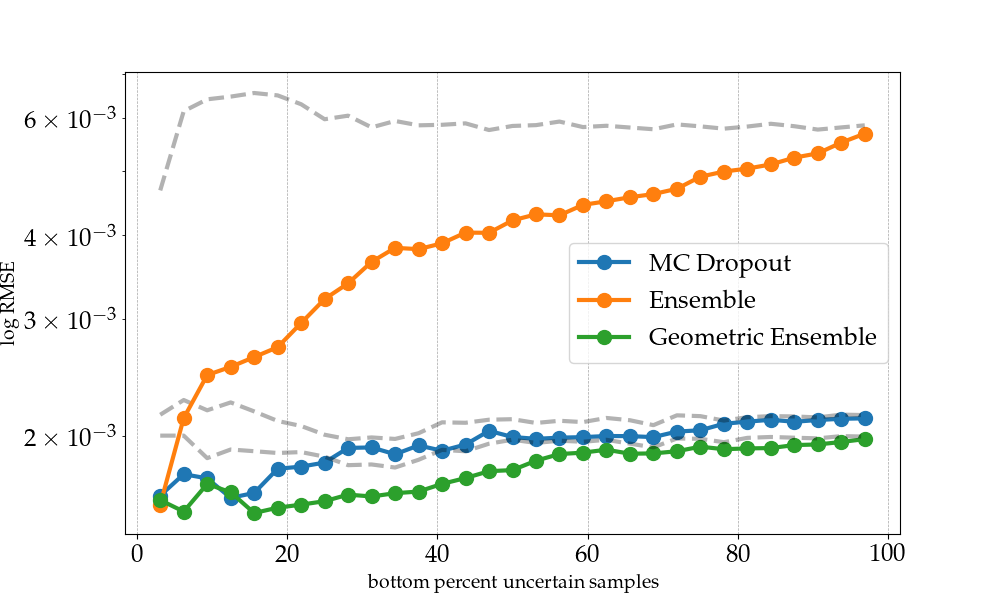
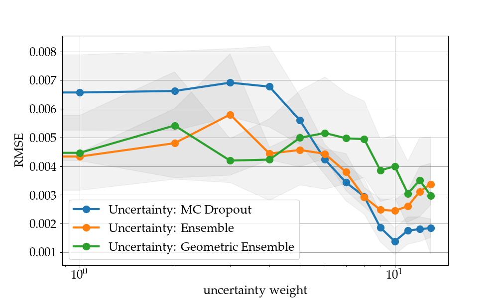
CRN on the COVID-19 dataset

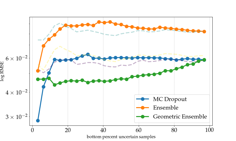
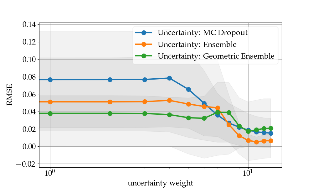
Figure 3: Comparison of the model-agnostic uncertainty quantification methods: MC dropout, ensemble and geometric ensemble methods applied to the CRN on the cardiovascular dataset (upper) and COVID-19 dataset (lower). Performance of treatment selection when varying the uncertainty estimate of the selected samples (left) and varying the uncertainty weight on the whole dataset (right). Selecting the least uncertain samples yields more reliable predictions of the outcome. On the left, we evaluate the models on an increasing percentage of the least uncertain samples (solid line) and compare this to a random subset of the validation data (dashed line). In all uncertainty-quantification methods, treatment selection yields more reliable treatments by increasing the weight on the uncertainty objective.

5 Conclusion

In this work, we propose a method to predict clinical outcomes and optimize treatment effects over time, leveraging uncertainty quantification techniques. Our approach improves on current counterfactual estimation techniques by handling continuous-valued treatment variables – dosages – which are common in real-world medical applications. The results from testing on two synthetic datasets show that the proposed method could be applied alongside counterfactual estimation techniques to improve the treatment selection process.

Our method’s ability to prioritize treatments that yield highly certain outcomes within a controlled treatment cost framework could be beneficial for personalized medicine: it ensures that the selected treatments are not only cost-effective but also minimize the potential risks associated with high-dose treatments. The added uncertainty component in the treatment selection process enhances decision-making, leading to more reliable patient care outcomes. The strength of our method lies in its robust performance across a range of uncertainty quantification models, counterfactual estimation techniques, and treatment parameters. Put together, its cost-effectiveness, reliability and robustness makes our proposed method well-suited to a variety of medical contexts, offering practitioners the flexibility to identify the optimal treatment approach. Future works could extent the method with additional uncertainty quantification methods and treatment constraints.

Appendix

Appendix A Counterfactual Estimation Baselines

We consider different counterfactual estimation methods in our models and compare their performance. In our implementations, we modify all methods to handle continuous-valued treatments.

• BNCDE [Hess et al., 2023]: The BNCDE method combines neural stochastic differential equations for Bayesian uncertainty quantification with neural controlled differential equations for continuous-time treatment effect estimation. Neural stochastic differential equations enable tractable variational Bayesian inference, allowing for the parameterization of posterior distributions of network weights. We build on the implementation by Hess et al. [2023], extending the method to continuous treatments. At inference time, we allow multi-step prediction by predicting outcomes from latents at several time steps, instead of the final time step.

• G-NET [Li et al., 2021]: G-Net is a sequential deep learning framework for counterfactual prediction based on g-computation. It leverages recurrent neural networks (RNNs) to model time-varying covariates and treatments in complex longitudinal data settings. G-Net estimates the effects of dynamic treatment strategies by simulating patient trajectories under alternative treatments. By employing RNNs, G-Net captures both temporal dependencies and non-linearities in the data, providing more accurate predictions compared to classical models, particularly for counterfactual predictions in clinical and simulated environments like cardiovascular simulations and tumor growth datasets. Our implementation of the G-NET uses GRU-RNNs and a common head for predicting outcomes and covariates.

• CT: The Causal Transformer (CT) is designed to estimate counterfactual outcomes over time by capturing long-range dependencies in time-series data, such as patient trajectories. The model incorporates three parallel transformer subnetworks that process different input sequences: time-varying covariates, past treatments, and past outcomes. These are fused using cross-attention to create a balanced representation. Additionally, CT uses Counterfactual Domain Confusion (CDC) loss to minimize confounding bias and produce reliable counterfactual predictions. We replace the CDC loss with the HSIC as a balancing criterion that is suitable for continuous-valued treatments (see Section …for more details).

• CRN: The Counterfactual Recurrent Network (CRN) is a sequence-to-sequence model designed for estimating treatment effects over time. It employs an encoder-decoder architecture where the encoder processes patient history, including time-varying covariates and past treatments, to generate a treatment-invariant representation. This representation is refined through adversarial training to minimize the influence of confounding variables. The decoder uses this balanced representation to predict outcomes under alternative treatment plans, allowing for reliable counterfactual estimations and treatment recommendations over time. We use HSIC for balancing representation loss for the considered continuous treatment setting (see Section …for more details) and GRU RNNs.

• CF-ODE: The Counterfactual ODE (CF-ODE) method models treatment effects over time and their epistemic uncertainty using an NSDE. The model encodes the observed time series into a latent space via a GRU RNN, and then integrates the hidden state forward in time using a treatment-specific processes within a NSDE. We extend this model to continuous-valued treatments by replacing the binary treatment-specific processes with an encoding of continuous-valued treatments. Specifically, we add the final hidden state of a GRU RNN processing the treatments to the hidden state to be integrated.

In our experiments, we apply Reversible Instance Normalization (RevIN) [Kim et al., 2021] to all settings, leading the input to be normalized at the start and denormalized at the output, ensuring consistency in data distributions and reducing the impact of distribution shifts between training and test sets.

Appendix B Temporal Confounding and Balancing Representation

When considering counterfactual estimation, time-varying confounding might lead to a bias in the treatment assignment $A_{0:t}$ in the observational distribution. This is usually referred to as confounding bias. Bica et al. [2020a], Melnychuk et al. [2022] use an adversarial objective to produce a sequence of balanced representations, which are simultaneously predictive of the outcome but non-predictive of the current treatment assignment, resulting in a treatment-invariant representation of the patient history $\Phi(\bar{\mathbf{h}}_{t}^{i})$, breaking the association between the treatment history and the treatment assignment. Bica et al. [2020a], Melnychuk et al. [2022] show that these representations can remove the bias from time-varying confounders. More specifically, they learn a representation such that $P(\Phi(\bar{\mathbf{h}}_{t})\mid\mathbf{A}_{t}=\mathbf{a}^{(k)})\quad\text{is equal for all}\quad k=1,2,\ldots,K$ treatments. The current adversarial-learning based methods of Bica et al. [2020a], Melnychuk et al. [2022] are built for discrete treatment variables. We extend this balancing objective to to learn a treatment invariant representation $\Phi(\bar{\mathbf{H}}_{t})$ to continuous-valued treatments. Instead of an adversarial loss with an auxiliary treatment classifier head, we encourage treatment invariant representations by minimizing the Hilbert-Schmidt independence criterion between past treatments and a representation of the trajectory $\text{HSIC}(\mathbf{A}_{t},\Phi(\bar{\mathbf{H}}_{t}))$. In contrast to adversarial losses, the HSIC is non-parametric and robust to class imbalance in treatments.

Table 1: Parameters for Cardiovascular Simulation

Parameter	Description	Value
$f_{hr_{\text{max}}}$	Maximum heart rate scaling factor	3.0
$f_{hr_{\text{min}}}$	Minimum heart rate scaling factor	0.6666
$r_{tpr_{\text{max}}}$	Maximum total peripheral resistance	2.134
$r_{tpr_{\text{min}}}$	Minimum total peripheral resistance	0.5335
$r_{tpr_{\text{mod}}}$	Modifier for total peripheral resistance	0.0
$sv_{\text{mod}}$	Stroke volume modification due to intervention (matches $\theta$)	0.001
$ca$	Arterial compliance	4.0
$cv$	Venous compliance	111.0
$k_{\text{width}}$	Width parameter for sigmoid function	0.1838
$p_{\text{aset}}$	Setpoint arterial pressure	70
$\tau$	Time constant for autonomic response	20
$p_{0\text{lv}}$	Left ventricular preload pressure	2.03
$r_{\text{valve}}$	Valve resistance	0.0025
$k_{\text{elv}}$	Left ventricular elastance coefficient	0.066
$v_{ed0}$	Initial end-diastolic volume	7.14
$T_{\text{sys}}$	Systole duration	0.2666
$cprsw_{\text{max}}$	Maximum pressure-volume relation (cprsw)	103.8
$cprsw_{\text{min}}$	Minimum pressure-volume relation (cprsw)	25.9

Table 2: Parameters for COVID-19 Dataset Simulation

Parameter	Description	Value
$hill_{\text{cure}}$	Hill coefficient for cure response	2.0
$h_{p}$	Hill coefficient for pathogen response	2.0
$k_{c_{p}}$	Half-maximal effective concentration for pathogen	1.0
$k_{ep}$	Maximum effect of pathogen response	1.0
$k_{d}$	Drug effect rate (pathogen-related)	1.0
$k_{dp}$	Disease progression rate	1.0
$k_{dr}$	Immunity-driven disease removal rate	1.0
$k_{di}$	Immune reaction to disease	1.0
$k_{id}$	Disease-induced immune response activation rate	1.0
$k_{if}$	Immune feedback rate	1.0
$k_{io}$	Immune response decay rate	1.0
$k_{im}$	Immunity buildup rate	1.0
$k_{kel}$	Drug elimination rate	1.0

We assess the performance of balancing representations on continuous-valued treatments. To model different levels of confounding, at the beginning of each treatment cycle $i$ we sample doses $\theta$ from a beta distribution parameterized as following Bica et al. [2020b]

$$\theta_{i+1}\sim\text{Beta}(\alpha,\beta),\quad\text{where }\beta=\frac{\alpha-1}{d_{w}^{i+1}}+2-\alpha\>.$$

For both data simulations, we set $d_{w}^{0}=\mathbf{A}_{0}$.

For the COVID-19 data simulation, we specify $d_{w}^{i+1}$ as

$$d_{w}^{i+1}=\begin{cases}d_{w}^{i}\times 1.1&\text{if }y_{0}^{i+1}\geq y_{0}^{i}\>,\\ d_{w}^{i}\times 0.9&\text{if }y_{t}^{i+1}\leq y_{0}^{i}\>.\end{cases}$$ (1)

For the cardiovascular data simulation, we do not specify $d_{w}^{i+1}$, but instead set $d_{w}^{i+1}=d_{w}^{i}=\ldots=d_{w}^{1}=\mathbf{A_{0}}$. When $\alpha=1$, the distribution becomes uniform, and so $\theta$ is independent of previous outcomes, treatments and covariates—preventing confounding entirely. Increasing $\alpha$ yields stronger confounding.

To check if balancing representations help in our settings, we set $\alpha=2$ and up-weigh the balancing objective in our loss, in factors of $\lambda$. In line with the literature Alaa and Schaar [2018], we find no benefit for $\lambda\geq 0$ in Figure 4.

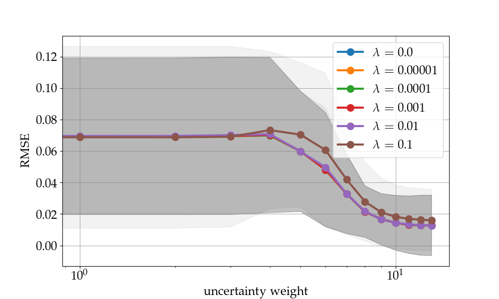
Figure 4: Encouraging a balancing representations with increasing weight on the HSIC objective has a negligible effect on reliable counterfactual estimation compared to the uncertainty objective

Appendix C Dataset Simulation

We sample the initial conditions of the cardiovascular dataset from the following distributions:

SV $$\sim\text{Unif}(0.9,1.0)\>,$$

$$P_{a} \sim\text{Unif}(0.75,0.85)\>,$$

$$P_{v} \sim\text{Unif}(0.3,0.7)\>,$$

$$s \sim\text{Unif}(0.15,0.25)\>.$$

and for the COVID-19 dataset:

$$Z_{i}\sim\text{Exp}(0.01)\quad\text{for }i\in\{1,2,3,4\}\>.$$

A more detailed overview of the parameters for the cardiovascular and COVID-19 datasets simulation can be found in Table 1 and Table 2 respectively.

Appendix D Experiments

D.1 Constraints on Treatment Trajectories

To ensure optimal treatment administration within a clinically acceptable framework, we use different constraints on the dosage trajectory ${\mathbf{A}}_{t:t+\tau}$ such that $S({\mathbf{A}}_{t:t+\tau})\subseteq\mathcal{A}$. This is achieved by applying a mapping $v:\mathbb{R}^{\tau\times d_{a}}\to S(\mathbf{A}_{t:t+\tau})$, where $v(\mathbf{A}_{t:t+\tau})\in S(\mathbf{\mathbf{A}}_{t:t+\tau})$.

• Range Clamping: Each dosage is adjusted to remain within a specified range, mitigating the risk of excessively high or low doses. This is implemented by centering and clamping the dosage values within the interval $[a,b]$

  $$v_{range}(\mathbf{A}_{t:t+\tau})=\min(\max(\mathbf{A}_{t:t+\tau}-\text{Mean}(\mathbf{A}_{t:t+\tau}),a),b)\>.$$

• Soft Clamping: To discourage extreme dosages while improving optimization, a soft clamping approach is applied, which pulls values towards a central range defined by $\beta$

  $$v_{soft}(A_{t:t+\tau})=\begin{cases}\alpha\mathbf{A}_{t:t+\tau}&\text{if }\mathbf{A}_{t:t+\tau}>\beta\>,\\ \mathbf{A}_{t:t+\tau}&\text{if }-\beta\leq\mathbf{A}_{t:t+\tau}\leq\beta\>,\\ \alpha\mathbf{A}_{t:t+\tau}&\text{if }\mathbf{A}_{t:t+\tau}<-\beta\>.\end{cases}$$

• $\tanh$ Clamping: To limit dosages within a range $(-\beta,\beta)$ while providing a continuous function, we apply the $\tanh$ clamping method

  $$v_{tanh}(\mathbf{A}_{t:t+\tau})=\beta\cdot\tanh(\mathbf{A}_{t:t+\tau})\>.$$

These constraints allow flexibility within defined clinical parameters for determining dosage administration constraints. These seemed the most realistic and interesting settings, however changes to these constraints can be made based on specific clinical needs or treatment goals.

Table 3: Parameters for Treatment Selection

Parameter	Value
Uncertainty Weights	$0$, $10^{-5}$, $10^{-4}$, $10^{-3}$, $10^{-2}$, $0.0625$, $0.125$, $0.25$, $0.5$, $1$, $2$, $4$, $8$, $16$
MSE Weight	$0.02$
Constraints	Soft clamp, $\beta=4$, $\alpha=0.01$
Optimizer	AdamW [Loshchilov and Hutter, 2019]
Optimization Steps	$50$
Learning Rate	$0.1$
Replicates	$6$

D.2 Experiment Details

We present the parameters used for treatment selection in Table 3.

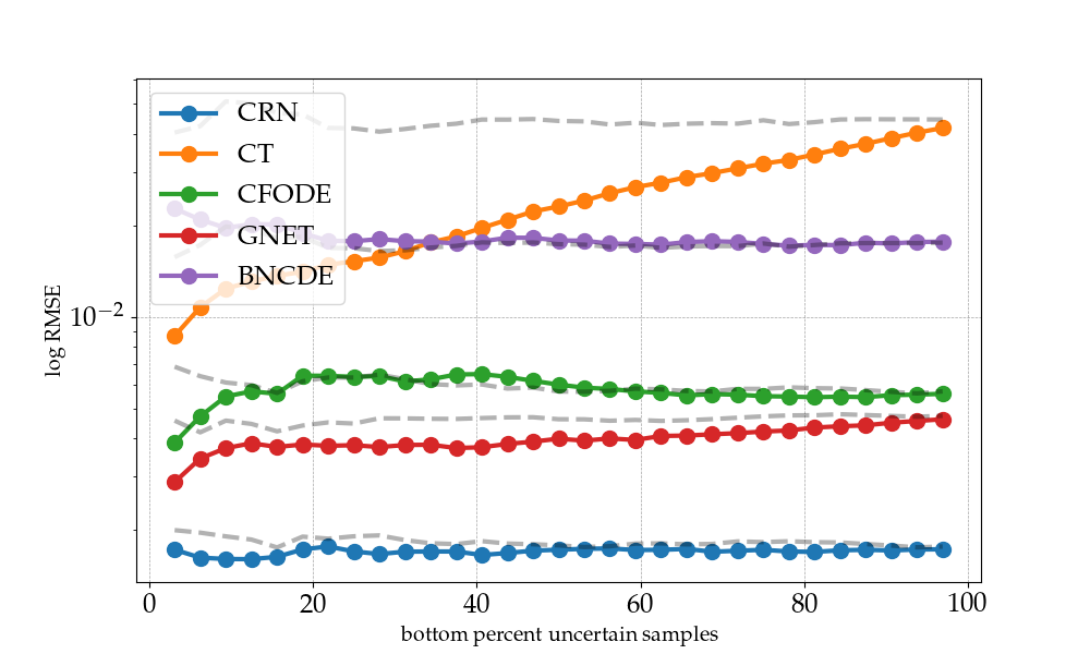
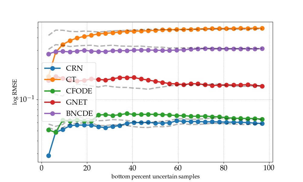
Figure 5: Performance comparison of the baseline models CRN, CT, CF-ODE, G-NET, BNCDE in treatments selection for cardiovascular (left) and COVID-19 (right) datasets. This comparison includes varying percentages of the most uncertain samples alongside a random subset of the validation data. The trends observed across different baselines are relatively stable, showing overall improved performance with increased certainty in the sample selection.

G-NET on the cardiovascular dataset

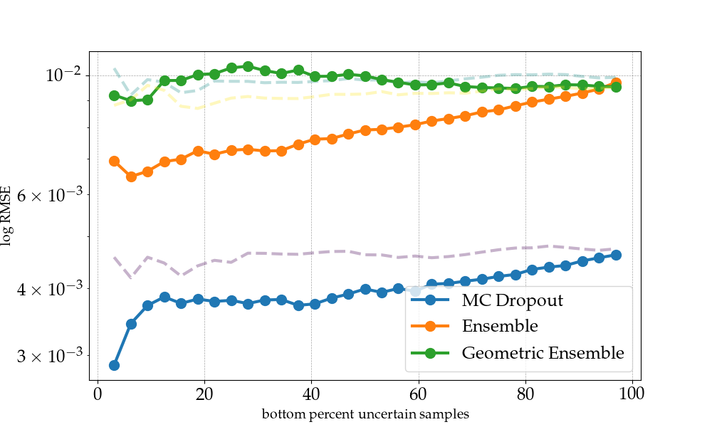
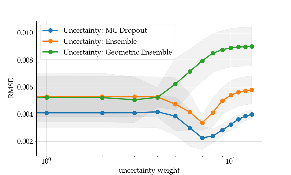
G-NET on the cardiovascular dataset

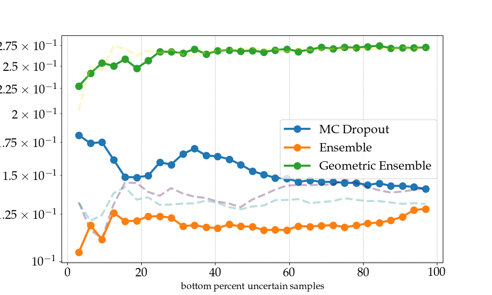
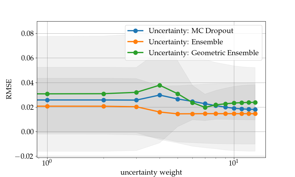
Figure 6: Comparison of the model-agnostic uncertainty quantification MC dropout, ensemble and geometric ensemble methods applied to the G-NET on the cardiovascular dataset (up) and COVID-19 dataset (low). Performance of treatment selection by varying the certainty of the selected samples (left) and by varying uncertainty weight on the whole dataset (right). Selecting the least uncertain samples yields more reliable predictions of the outcome. We evaluate the models on an increasing percentage of the least uncertain samples together with a random subset of the validation data.

D.3 Additional Experiments

We also show more results with the different counterfactual estimation baselines in Figure 5 and we assess the performance of the method with different uncertainty quantification methods with an additional model – the G-NET – in Figure 6.

References

- Alaa and Schaar (2018) Ahmed Alaa and Mihaela Schaar. Limits of estimating heterogeneous treatment effects: Guidelines for practical algorithm design. In International Conference on Machine Learning, pages 129–138. PMLR, 2018.
- Allam et al. (2021) Ahmed Allam, Stefan Feuerriegel, Michael Rebhan, and Michael Krauthammer. Analyzing patient trajectories with artificial intelligence. Journal of medical internet research, 23(12):e29812, 2021.
- Auger et al. (2005) R. Robert Auger, Scott H. Goodman, Michael H. Silber, Lois E. Krahn, V. Shane Pankratz, and Nancy L. Slocumb. Risks of High-Dose Stimulants in the Treatment of Disorders of Excessive Somnolence: A Case-Control Study. Sleep, 28(6):667–672, 06 2005. ISSN 0161-8105. doi: 10.1093/sleep/28.6.667. URL https://doi.org/10.1093/sleep/28.6.667.
- Bellos (2023) Ioannis Bellos. Multicriteria decision-making methods for optimal treatment selection in network meta-analysis. Medical Decision Making, 43(1):78–90, 2023.
- Bica et al. (2020a) Ioana Bica, Ahmed M Alaa, James Jordon, and Mihaela van der Schaar. Estimating counterfactual treatment outcomes over time through adversarially balanced representations. In International Conference on Learning Representations, 2020a. URL https://openreview.net/forum?id=BJg866NFvB.
- Bica et al. (2020b) Ioana Bica, James Jordon, and Mihaela van der Schaar. Estimating the effects of continuous-valued interventions using generative adversarial networks. Advances in Neural Information Processing Systems, 33:16434–16445, 2020b.
- Brouwer et al. (2022) Edward De Brouwer, Javier González Hernández, and Stephanie Hyland. Predicting the impact of treatments over time with uncertainty aware neural differential equations, 2022. URL https://arxiv.org/abs/2202.11987.
- Caye et al. (2019) Arthur Caye, James M Swanson, David Coghill, and Luis Augusto Rohde. Treatment strategies for adhd: an evidence-based guide to select optimal treatment. Molecular psychiatry, 24(3):390–408, 2019.
- Curth and van der Schaar (2021) Alicia Curth and Mihaela van der Schaar. Nonparametric estimation of heterogeneous treatment effects: From theory to learning algorithms. In International Conference on Artificial Intelligence and Statistics, pages 1810–1818. PMLR, 2021.
- Dai et al. (2021) Wei Dai, Rohit Rao, Anna Sher, Nessy Tania, Cynthia J Musante, and Richard Allen. A prototype qsp model of the immune response to sars-cov-2 for community development. CPT: pharmacometrics & systems pharmacology, 10(1):18–29, 2021.
- Dienstmann et al. (2015) Rodrigo Dienstmann, Ramon Salazar, and Josep Tabernero. Personalizing colon cancer adjuvant therapy: selecting optimal treatments for individual patients. Journal of clinical oncology, 33(16):1787–1796, 2015.
- Feuerriegel et al. (2024) Stefan Feuerriegel, Dennis Frauen, Valentyn Melnychuk, Jonas Schweisthal, Konstantin Hess, Alicia Curth, Stefan Bauer, Niki Kilbertus, Isaac S Kohane, and Mihaela van der Schaar. Causal machine learning for predicting treatment outcomes. Nature Medicine, 30(4):958–968, 2024.
- Frei III and Canellos (1980) Emil Frei III and George P Canellos. Dose: a critical factor in cancer chemotherapy. The American journal of medicine, 69(4):585–594, 1980.
- Gal and Ghahramani (2016) Yarin Gal and Zoubin Ghahramani. Dropout as a bayesian approximation: Representing model uncertainty in deep learning. In international conference on machine learning, pages 1050–1059. PMLR, 2016.
- Garipov et al. (2018) Timur Garipov, Pavel Izmailov, Dmitrii Podoprikhin, Dmitry Vetrov, and Andrew Gordon Wilson. Loss surfaces, mode connectivity, and fast ensembling of dnns, 2018. URL https://arxiv.org/abs/1802.10026.
- Hess et al. (2023) Konstantin Hess, Valentyn Melnychuk, Dennis Frauen, and Stefan Feuerriegel. Bayesian neural controlled differential equations for treatment effect estimation. arXiv preprint arXiv:2310.17463, 2023.
- Johansson et al. (2022) Fredrik D Johansson, Uri Shalit, Nathan Kallus, and David Sontag. Generalization bounds and representation learning for estimation of potential outcomes and causal effects. The Journal of Machine Learning Research, 23(1):7489–7538, 2022.
- Kallus and Zhou (2018) Nathan Kallus and Angela Zhou. Policy evaluation and optimization with continuous treatments. In International conference on artificial intelligence and statistics, pages 1243–1251. PMLR, 2018.
- Kerr et al. (2008) Eve A Kerr, Brian J Zikmund-Fisher, Mandi L Klamerus, Usha Subramanian, Mary M Hogan, and Timothy P Hofer. The role of clinical uncertainty in treatment decisions for diabetic patients with uncontrolled blood pressure. Annals of internal medicine, 148(10):717–727, 2008.
- Kim et al. (2021) Taesung Kim, Jinhee Kim, Yunwon Tae, Cheonbok Park, Jang-Ho Choi, and Jaegul Choo. Reversible instance normalization for accurate time-series forecasting against distribution shift. In International Conference on Learning Representations, 2021.
- Kreif et al. (2015) Noémi Kreif, Richard Grieve, Iván Díaz, and David Harrison. Evaluation of the effect of a continuous treatment: a machine learning approach with an application to treatment for traumatic brain injury. Health economics, 24(9):1213–1228, 2015.
- Li et al. (2021) Rui Li, Stephanie Hu, Mingyu Lu, Yuria Utsumi, Prithwish Chakraborty, Daby M. Sow, Piyush Madan, Jun Li, Mohamed Ghalwash, Zach Shahn, and Li-wei Lehman. G-net: a recurrent network approach to g-computation for counterfactual prediction under a dynamic treatment regime. In Subhrajit Roy, Stephen Pfohl, Emma Rocheteau, Girmaw Abebe Tadesse, Luis Oala, Fabian Falck, Yuyin Zhou, Liyue Shen, Ghada Zamzmi, Purity Mugambi, Ayah Zirikly, Matthew B. A. McDermott, and Emily Alsentzer, editors, Proceedings of Machine Learning for Health, volume 158 of Proceedings of Machine Learning Research, pages 282–299. PMLR, 04 Dec 2021. URL https://proceedings.mlr.press/v158/li21a.html.
- Lim (2018) Bryan Lim. Forecasting treatment responses over time using recurrent marginal structural networks. Advances in neural information processing systems, 31, 2018.
- Linial et al. (2021) Ori Linial, Neta Ravid, Danny Eytan, and Uri Shalit. Generative ode modeling with known unknowns. In Proceedings of the Conference on Health, Inference, and Learning, pages 79–94, 2021.
- Liu et al. (2023) Ruoqi Liu, Katherine M Hunold, Jeffrey M Caterino, and Ping Zhang. Estimating treatment effects for time-to-treatment antibiotic stewardship in sepsis. Nature machine intelligence, 5(4):421–431, 2023.
- Loshchilov and Hutter (2019) Ilya Loshchilov and Frank Hutter. Decoupled weight decay regularization, 2019. URL https://arxiv.org/abs/1711.05101.
- Lou et al. (2018) Zhilan Lou, Jun Shao, and Menggang Yu. Optimal treatment assignment to maximize expected outcome with multiple treatments. Biometrics, 74(2):506–516, 2018.
- Lu et al. (2013) Wenbin Lu, Hao Helen Zhang, and Donglin Zeng. Variable selection for optimal treatment decision. Statistical methods in medical research, 22(5):493–504, 2013.
- Melnychuk et al. (2022) Valentyn Melnychuk, Dennis Frauen, and Stefan Feuerriegel. Causal transformer for estimating counterfactual outcomes. In Kamalika Chaudhuri, Stefanie Jegelka, Le Song, Csaba Szepesvari, Gang Niu, and Sivan Sabato, editors, Proceedings of the 39th International Conference on Machine Learning, volume 162 of Proceedings of Machine Learning Research, pages 15293–15329. PMLR, 17–23 Jul 2022. URL https://proceedings.mlr.press/v162/melnychuk22a.html.
- Melnychuk et al. (2023) Valentyn Melnychuk, Dennis Frauen, and Stefan Feuerriegel. Bounds on representation-induced confounding bias for treatment effect estimation. arXiv preprint arXiv:2311.11321, 2023.
- Moodie et al. (2007) Erica EM Moodie, Thomas S Richardson, and David A Stephens. Demystifying optimal dynamic treatment regimes. Biometrics, 63(2):447–455, 2007.
- Murphy (2003) Susan A Murphy. Optimal dynamic treatment regimes. Journal of the Royal Statistical Society Series B: Statistical Methodology, 65(2):331–355, 2003.
- Polley and van der Laan (2009) Eric C Polley and Mark J van der Laan. Selecting optimal treatments based on predictive factors. In Design and Analysis of Clinical Trials with Time-to-Event Endpoints, pages 459–472. Chapman and Hall/CRC, 2009.
- Qian et al. (2021) Zhaozhi Qian, William Zame, Lucas Fleuren, Paul Elbers, and Mihaela van der Schaar. Integrating expert odes into neural odes: pharmacology and disease progression. Advances in Neural Information Processing Systems, 34:11364–11383, 2021.
- Robins et al. (2004) James M Robins, DY Lin, and PJ Heagerty. Optimal structural nested models for optimal sequential decisions. Proceedings of the second Seattle symposium in biostatistics, pages 189–326, 2004.
- Rubin (2005) Donald B Rubin. Causal inference using potential outcomes: Design, modeling, decisions. Journal of the American Statistical Association, 100(469):322–331, 2005.
- Seedat et al. (2022) Nabeel Seedat, Fergus Imrie, Alexis Bellot, Zhaozhi Qian, and Mihaela van der Schaar. Continuous-time modeling of counterfactual outcomes using neural controlled differential equations. In Kamalika Chaudhuri, Stefanie Jegelka, Le Song, Csaba Szepesvari, Gang Niu, and Sivan Sabato, editors, Proceedings of the 39th International Conference on Machine Learning, volume 162 of Proceedings of Machine Learning Research, pages 19497–19521. PMLR, 17–23 Jul 2022. URL https://proceedings.mlr.press/v162/seedat22b.html.
- Shalit et al. (2017) Uri Shalit, Fredrik D Johansson, and David Sontag. Estimating individual treatment effect: generalization bounds and algorithms. In International conference on machine learning, pages 3076–3085. PMLR, 2017.
- Song et al. (2015) Rui Song, Michael Kosorok, Donglin Zeng, Yingqi Zhao, Eric Laber, and Ming Yuan. On sparse representation for optimal individualized treatment selection with penalized outcome weighted learning. Stat, 4(1):59–68, 2015.
- Utomo et al. (2018) Chandra Prasetyo Utomo, Xue Li, and Weitong Chen. Treatment recommendation in critical care: A scalable and interpretable approach in partially observable health states. In International Conference on Interaction Sciences, 2018. URL https://api.semanticscholar.org/CorpusID:54443065.
- van Geloven et al. (2020) Nan van Geloven, Sonja A Swanson, Chava L Ramspek, Kim Luijken, Merel van Diepen, Tim P Morris, Rolf HH Groenwold, Hans C van Houwelingen, Hein Putter, and Saskia le Cessie. Prediction meets causal inference: the role of treatment in clinical prediction models. European journal of epidemiology, 35:619–630, 2020.
- Weiting et al. (2022) Huang Weiting, Alwin Zhang Yaoxian, Yeo Khung Keong, Shao Wei Lam, Lau Yee How, Anders Olof Sahlén, Ahmadreza Pourghaderi, Matthew Che, Chua Siang Jin Terrance, and Nicholas Graves. The clinical value and cost-effectiveness of treatments for patients with coronary artery disease. Health Economics Review, 12(1):1–8, 2022.
- West and West (2002) Andrew F West and RR West. Clinical decision-making: coping with uncertainty, 2002.
- Zenker et al. (2007) Sven Zenker, Jonathan Rubin, and Gilles Clermont. From inverse problems in mathematical physiology to quantitative differential diagnoses. PLoS computational biology, 3(11):e204, 2007.
- Zhang et al. (2012) Baqun Zhang, Anastasios A Tsiatis, Marie Davidian, Min Zhang, and Eric Laber. Estimating optimal treatment regimes from a classification perspective. Stat, 1(1):103–114, 2012.