Generalised logistic regression with vine copulas

Abstract

We propose a generalisation of the logistic regression model, that aims to account for non-linear main effects and complex interactions, while keeping the model inherently explainable. This is obtained by starting with log-odds that are linear in the covariates, and adding non-linear terms that depend on at least two covariates. More specifically, we use a generative specification of the model, consisting of a combination of certain margins on natural exponential form, combined with vine copulas. The estimation of the model is however based on the discriminative likelihood, and dependencies between covariates are included in the model, only if they contribute significantly to the distinction between the two classes. Further, a scheme for model selection and estimation is presented. The methods described in this paper are implemented in the R package LogisticCopula. In order to assess the performance of our model, we ran an extensive simulation study. The results from the study, as well as from a couple of examples on real data, showed that our model performs at least as well as natural competitors, especially in the presence of non-linearities and complex interactions, even when $n$ is not large compared to $p$.

1 Introduction

The logistic regression model is ubiquitous in discriminative modelling, where the interest is a conditional model for a binary outcome variable $Y$, given an observation of a $p$-dimensional covariate vector $\mathbf{X}$. The logistic regression model in its simplest form is given by

$$\log\left(\frac{P(Y=1|\mathbf{X}=\mathbf{x})}{P(Y=0|\mathbf{X}=\mathbf{x})}\right)=\beta_{0}+\mathbf{x}^{t}\bm{\beta},$$ (1)

i.e., the model for the log-odds ratio is linear. The model parameters are then estimated using the conditional likelihood of $Y|\mathbf{X}=\mathbf{x}$. This model also has the advantage that it is inherently interpretable. For instance, the decision to accept or deny can be explained to a layperson applying for a bank loan through how the prediction depends on whether a weighed sum of factors such as their age, level of education, number of children, etc., exceeds a certain threshold, i.e. the decision boundary. This is important particularly when used for applications that are affected by regulations on transparency, such as the General Data Protection Regulation (GDPR) of the EU, which states that any data subject (a person, a company, etc.) has the right to ‘an explanation of the decision reached after [algorithmic] assessment’ [Goodman and Flaxman, 2016].

The logistic regression model is a typical example of a discriminative framework, where the parameters are estimated by maximising the conditional likelihood of $Y|\mathbf{X}=\mathbf{x}$. An alternative is to use generative models for discrimination. The model for $Y$ given $\mathbf{X}=\mathbf{x}$ is then specified indirectly via the conditional distributions of $\mathbf{X}|Y=y$ for $y=0,1$ and the marginal probability $\pi_{Y}=P(Y=1)$, as

$$P(Y=1|\mathbf{x})=\left(\pi_{Y}p(\mathbf{x}|Y=1)\right)/\left((1-\pi_{Y})p(\mathbf{x}|Y=0)+\pi_{Y}p(\mathbf{x}|Y=1)\right).$$ (2)

If one models $\mathbf{X}|Y=y$ with the multivariate Gaussian distribution, the result is a linear or quadratic discriminative model, whereas the Naive Bayes model is defined by the assumption that the $X_{i}$s are conditionally independent given $Y$. In this setting, the parameters are estimated via the likelihood functions of $\mathbf{X}|Y=y$ separately for the two classes.

Restricted to certain choices of marginal distributions, Naive Bayes models lead to log-odds that are linear in the covariates. Hence, such a model is in some sense equivalent to a logistic regression model, apart from how the parameters are estimated. Several publications compare discriminative and generative models that are equivalent in that sense, e.g. Efron [1975], O’Neill [1980], Rubinstein and Hastie [1997] and Ng and Jordan [2002]. While it is true that linear discriminant analysis is asymptotically efficient compared to logistic regression, and that generative models such as a Naive Bayes model often works surprisingly well for small sample problems, for most applications where at least a moderate amount of training data is available, a discriminative model is preferable. Sometimes, it may be possible to construct a model that gives better predictions than the simple logistic regression. However, one should acknowledge that model mechanics that are comprehensible to a human have an inherent value in many applications, for instance for stakeholders who need to trust that the model predictions make sense - and for subjects who need to trust that a model-based or model-assisted decision that affects them is not subjecting them to unlawful discrimination.

In this paper, we generalise the logistic regression model to account for non-linear main effects and interaction effects, in order to improve prediction performance, but in such a way that the inherent interpretability of the logistic regression model is kept. We do this by using a specification of the model on generative form. More specifically, we set up a model for each of the two classes as a combination of certain marginal distributions and a vine copula [Joe, 1997, Bedford and Cooke, 2001, 2002, Kurowicka and Cooke, 2006a, Aas et al., 2009], accounting for the dependence. The resulting model for the log odds becomes a sum of the logistic regression model (1) with linear main effects and non-linear terms that involve two covariates or more. The idea is that the logistic regression part will provide most of the explanation of a particular outcome, whereas the added, more complex non-linear terms improve the predictions, similar to the idea behind Glad [2001] for linear regression. This is akin to interpretable machine learning, which focuses on creating models that are in themselves more understandable to a human, as opposed to explainable artificial intelligence, that attempts to ’explain’ a decision made by a model using for instance simple(r) approximations of the model [Rudin et al., 2022]. We think that in applications where explainability is valuable and the simple linear log-odds provides an insufficiently good fit, our way of constructing models is more responsible, compared to employing for instance a combination of boosted tree models, or deep neural nets, and an exogenous explanation, since there must be a discrepancy between what the model computes and the explanation of the model, and therefore cases where the explanation is wrong, or else the entire model could be replaced by its explanation [Rudin, 2019].

Specifically, we construct our model starting from a Naive Bayes model resulting in linear log odds, and then add vine copula terms [Joe, 1997, Bedford and Cooke, 2001, 2002, Kurowicka and Cooke, 2006a, Aas et al., 2009] which introduce additional non-linear effects and interaction terms in the form of between - covariate dependence, conditional on the response. The resulting model for the log odds ratio becomes a sum of the logistic regression model (1) with linear main effects and some non-linear terms that involve two covariates or more. While we construct the form of our model based on a generative model specification, the parameters are found by maximising the discriminative likelihood of $Y|\mathbf{X}=\mathbf{x}.$ Other models that could be seen in this context are Bien et al. [2013] and Lim and Hastie [2015], that add pairwise interactions as products of covariates using group-lasso. Compared to those, our model is more flexible, as it also allows more complex interactions, both in terms of functional form and order of interaction. Anecdotally, for one of the data examples, our method resulted in a model that had fewer interaction terms than the group- lasso method, but yielded similar predictions out of sample.

Our model can also be seen as an extension of a Naive Bayes model, by including dependence in the form of a vine copula, which has already been attempted, see for instance Vogelaere [2020]. A major difference in the framework we propose is it uses the discriminative likelihood-based estimators and not the generative ones. Further, dependence between certain covariates is only included when it differs sufficiently in the two classes. Hence, the purpose is not to model the distribution of the covariates in the two classes as well as possible, but to make the best possible model to discriminate between the two classes.

The paper is organised as follows. Section 2 describes the proposed extension of the logistic regression model. The methods for estimation and model selection are presented in Section 3. These first parts of the paper focus on continuous covariates, whereas the necessary modifications in order to include discrete covariates are given in Section 4. In Section 5, we assess the characteristics of the proposed model and compare it to related alternatives, and in Section 6, we illustrate it on two real data examples. Finally, we make some concluding remarks in Section 7.

2 Extending the logistic regression model

As mentioned earlier, our aim is to extend the logistic regression model in its simplest form via a generative model specification. We will here assume that all covariates $X_{j}$ are continuous, but our model can easily be adapted to also handle discrete covariates, as discussed in Section 4.

We start by specifying a Naive Bayes type model, i.e., assuming conditional independence between the covariates $\mathbf{X}$ given $Y$, where the marginal distributions of the covariates are such that the resulting log-odds ratio is linear in $\mathbf{X}$ as in (1). Using (2) with $p(\mathbf{x}|Y=y)=\prod_{j=1}^{p}p(x_{j}|Y=y)$, the log-odds ratio becomes

$$\log\left(\frac{P(Y=1|\mathbf{x})}{P(Y=0|\mathbf{x})}\right) =\log\left(\frac{\pi_{Y}}{1-\pi_{Y}}\right)+\sum_{j=1}^{p}\log\left(\frac{p\left(x_{j}|Y=1\right)}{p\left(x_{j}|Y=0\right)}\right).$$

This means that the marginal distributions $p(x_{j}|Y=y)$ need to be such that $\log(p\left(x_{j}|Y=1\right)/p\left(x_{j}|Y=0\right))=a_{j}+b_{j}x_{j}$ for some constants $a_{j}$ and $b_{j}$. This is fulfilled by members of the natural exponential family [Morris, 1982, Cox and Snell, 1989], and we therefore choose to model the covariates as $\left[X_{j}|Y=y\right]\sim N(\mu_{y,j},\sigma_{j}^{2})$, i.e $p\left(x_{j}|Y=y\right)=1/(\sqrt{2\pi}\sigma_{j})\exp\left(-1/(2\sigma_{j}^{2})(x_{j}-\mu_{y,j})^{2}\right)$, so that

$$\log\left(\frac{p(x_{j}|Y=1)}{p(x_{j}|Y=0)}\right)=\frac{1}{2}\left(\frac{\mu_{0,j}^{2}-\mu_{1,j}^{2}}{\sigma_{j}^{2}}\right)+\left(\frac{\mu_{1,j}-\mu_{0,j}}{\sigma_{j}^{2}}\right)x_{j}.$$

The resulting log-odds is of the form (1) with coefficients

$$\begin{split}\beta_{0}&=\log\left(\frac{\pi_{Y}}{1-\pi_{Y}}\right)+\sum_{j=1}^{p}\frac{1}{2}\left(\frac{\mu_{0,j}^{2}-\mu_{1,j}^{2}}{\sigma_{j}^{2}}\right)\\ \beta_{j}&=(\mu_{1,j}-\mu_{0,j})/\sigma_{j}^{2},\quad j=1,\ldots,p.\end{split}$$ (3)

Note that alternative marginal distributions for continuous covariates could also be used, such as an exponential distribution with a class-dependent parameter for covariates with support on the positive real numbers.

2.1 Extension with vine copulas

Our aim is to extend the above logistic regression model (1) to account for non-linear main effects, as well as potentially complex interaction effects in the log odds. In order to achieve that, we use the generative representation (2) of the model, introducing conditional dependence between (some of) the covariates in the form of a vine copula, but estimate the model parameters by maximising the likelihood of $Y|\mathbf{X}=\mathbf{x}$.

2.1.1 Vine copulas

A copula $C$ may be used to describe and analyse multivariate distributions, and is a multivariate distribution function whose univariate marginal distributions are all uniform. It allows to separate the distribution into two parts, a set of univariate marginal distributions, and the dependence structure. Indeed, Sklar’s theorem [Sklar, 1959] states that if the variables $X_{1},\dots,X_{d}$ are all continuous (which will be the case in the parts of the model where we introduce copulas), the joint probability density function (pdf) is given by

$$f(x_{1},\dots,x_{d})=f_{1}(x_{1})\cdot\ldots\cdot f_{d}(x_{d})\cdot c(F_{1}(x_{1}),\dots,F_{d}(x_{d})),$$

where $F_{1},\dots,F_{d}$ and $f_{1},\dots,f_{d}$ are the marginal cumulative distribution functions (cdf) and pdfs, respectively, and $c(u_{1},\dots,u_{d})=\partial^{d}C(u_{1},\dots,u_{p})/(\partial u_{1}\ldots\partial u_{d})$ ia the density of the unique copula $C$ of $X_{1},\dots,X_{d}$.

A very flexible, yet computationally tractable family of copulas are vine copulas [Joe, 1996, Bedford and Cooke, 2001, 2002, Kurowicka and Cooke, 2006a, Aas et al., 2009]. These models combine bivariate components, pair-copulas, into a multivariate copula, and are incredibly flexible, as all the involved pair-copulas can be selected completely freely [Joe et al., 2010].

Vine copulas consist of a sequence of trees $T_{i}$ with nodes $N_{i}$ and edges $E_{i}$, for $i=1,...,d-1$, where each edge corresponds to one of the pair-copulas that are the building blocks of the joint, multivariate copula. They satisfy the following conditions [Kurowicka and Cooke, 2006b]:

1. $T_{1}$ has nodes $N_{1}=\{1,...,d\}$ and edges $E_{1}$.

2. For $i=2,...,d-1$, $T_{i}$ has nodes $N_{i}=E_{i-1}$.

3. Proximity condition: two edges in tree $T_{i}$ can only be joined by an edge in tree $T_{i+1}$ if they share a common node in $T_{i}$.

Let $N_{ik}$ and $N_{il}$ be two nodes that are joined by the edge $e$ in $T_{i}$. Then, the proximity condition states that $N_{ij}$ and $N_{ik}$ must share all but one node, i.e. $N_{ij}=\{j(e),D(e)\}$ and $N_{ik}=\{k(e),D(e)\}$, where $D(e)$ are the nodes they have in common, called the conditioning set, and $j(e)$ and $k(e)$ the ones that are not shared, denoted the conditioned nodes. The edge $e$ is then associated with the bivariate copula $C_{j(e),k(e)|D(e)}$.

The density of a vine copula for a d-dimensional random vector $\mathbf{X}$ with marginal distributions $F_{1},\ldots,F_{d}$ is given by a product of $d(d-1)/2$ bivariate copula densities, and may be written as

$$c_{1\dots d}(F_{1}(x_{1}),\ldots, F_{d}(x_{d}))=\prod_{t=1}^{d-1}\prod_{e\in E_{t}}c_{j(e),k(e)|D(e)}\left(u_{j(e)|D(e)},u_{k(e)|D(e)}\right),$$ (4)

where $u_{j|D}=F(x_{j}|\mathbf{x}_{D}),$ and $\mathbf{X}_{D(e)}$ is the subvector of $\mathbf{X}$ determined by the indices $D(e)$. An example of a vine copula in dimension $5$ is shown in Figure 1, which has density

$$c_{1\ldots 5}=c_{12}\cdot c_{13}\cdot c_{14}\cdot c_{35}\cdot c_{34|1}\cdot c_{23|1}\cdot c_{15|3}\cdot c_{24|13}\cdot c_{25|13}\cdot c_{45|123},$$

where arguments are omitted for simplicity. In the first tree, these arguments are the univariate marginal distributions, and in subsequent trees, they are conditional distributions, where the number of variables conditioned on is equal to the tree number minus one. In vine copulas, these conditional distributions are easily computed based on pair-copulas from earlier trees, due to the proximity condition (see for instance (2) in the supplementary material). For a more comprehensive introduction to vine copulas, consult for instance Czado [2019].

Figure 1: Example of a vine copula for five variables.

2.1.2 Extension of logistic regression

In order to take non-linearities and possibly complex interaction effects into account, while maintaining an interpretable model, we allow some of the covariates to be conditionally dependent given the class $Y$, whereas the remaining covariates are conditionally independent. Now, the joint pdf for $\mathbf{X}|Y=y$ becomes

$$p(\mathbf{x}|Y=y)=\prod_{j=1}^{p}p(x_{j}|y)\cdot c^{y}(F_{1|y}(x_{1}|y),F_{2|y}(x_{2}|y),\dots,F_{p|y}(x_{p}|y)),$$

where $c^{y}$ is the copula density of the covariates in class $Y=y$. Letting $\bm{\mu}_{y}=(\mu_{y,1},\ldots,\mu_{y,p})$, $\bm{\sigma}=(\sigma_{1},\ldots,\sigma_{p})$ and $\beta_{j}$, $j=0,\ldots,p$, be as in (3), we can express the log-odds as an extension of (1):

$$\begin{split}\log\left(\frac{P(Y=1|\mathbf{X}=\mathbf{x})}{P(Y=0|\mathbf{X}=\mathbf{x})}\right)=&\beta_{0}+\sum_{j=1}^{p}\beta_{j}x_{j}+g(x_{1},\ldots,x_{p};\bm{\mu}_{0},\bm{\mu}_{1},\bm{\sigma},\bm{\theta}_{0},\bm{\theta}_{1}),\end{split}$$ (5)

where $\bm{\theta}_{0}$ and $\bm{\theta}_{1}$ are the parameters of the copulas $c^{0}$ and $c^{1}$ and $g(\cdot)$ is given by the difference in the logarithm of their densities. The idea is then to let $c^{0}$ and $c^{1}$ be vine copulas, meaning that $c^{i}$, $i=0,1$ are given by (4), resulting in

$$\begin{split}g(x_{1},\ldots,x_{p};\bm{\mu}_{0},\bm{\mu}_{1},\bm{\sigma},\bm{\theta}_{0},\bm{\theta}_{1})=\sum_{t=1}^{p-1}&\sum_{e\in E_{t}}\left(\log\left(c_{j(e),k(e)|D(e)}^{1}\left(u_{j(e)|D(e)}^{1},u_{k(e)|D(e)}^{1});\bm{\theta}_{j(e),k(e)|D(e)}^{1}\right)\right)\right.\\ &\ \ \ \ -\left.\log\left(c_{,j(e),k(e)|D(e)}^{0}\left(u_{j(e)|D(e)}^{0},u_{k(e)|D(e)}^{0};\bm{\theta}_{j(e),k(e)|D(e)}^{0}\right)\right)\right).\end{split}$$ (6)

Here, $u^{y}_{j(e)|D(e)}=F_{j(e)|D(e)}^{y},$ and $F_{j(e)|D(e)}^{y}$ is the cdf of $[X_{j(e)}|\mathbf{X}_{D(e)}=\mathbf{x}_{D(e)},Y=y]$, that depends on the marginal parameters $\bm{\mu}_{y}$ and $\bm{\sigma}$ as $F_{j(e)}^{i}(x_{j(e)})=F_{j(e)|y}(x_{j(e)}|y=i)=\Phi((x_{j(e)}-\mu_{i,j(e)})/\sigma_{j(e)})$ when $D(e)$ is empty, and also on copulas from earlier levels when it is not empty. Further, $c_{j(e),k(e)|D(e)}^{y}$ is the copula density linking $X_{j(e)}$ and $X_{k(e)}$, given $\mathbf{X}_{D(e)}=\mathbf{x}_{D(e)}$ and $Y=y$, and the pair-copula parameters $\bm{\theta}_{j(e),k(e)|D(e)}^{y}$ constitute $\bm{\theta}_{y}$. The terms of $g$ above are then important only if the difference between the two log-copula densities $c_{j(e),k(e)|D(e)}^{1}$ and $c_{j(e),k(e)|D(e)}^{0}$ is of a certain size. The point now is to keep only the copula pairs where this difference really contributes to the discrimination between the two classes, while setting the remaining copula densities to $1$, corresponding to (conditional) independence between $X_{j(e)}$ and $X_{k(e)}$ given $\mathbf{X}_{D(e)}=\mathbf{x}_{D(e)}$ in both classes.

As an example, assume that the function $g$ is given by

$$\log\left(c_{12}^{1}\right)-\log\left(c_{12}^{0}\right)+\log\left(c_{13}^{1}\right)-\log\left(c_{13}^{1}\right)+\log\left(c_{14}^{1}\right)-\log\left(c_{14}^{0}\right)$$

$$+ \log\left(c_{34|1}^{1}\right)-\log\left(c_{34|1}^{0}\right)+\log\left(c_{23|1}^{1}\right)-\log\left(c_{23|1}^{0}\right)+\log\left(c_{24|13}^{1}\right)-\log\left(c_{24|13}^{0}\right),$$

where the parameters and function arguments are omitted to simplify the notation. This corresponds to $c^{0}$ and $c^{1}$ being given by the vine in Figure 1, but where the copulas $c_{35}$, $c_{15|3}$, $c_{25|13}$ and $c_{45|123}$ are set to independence in both classes. If all $12$ copulas in the above expression are Gaussian, the resulting model (5) contains pairwise interactions between all the pairs constituting the conditioned sets of the above copulas, i.e. $(1,2)$, $(1,3)$, $(1,4)$, $(3,4)$, $(2,3)$ and $(2,4)$. This is a quadratic discriminative model, with different mean vectors in the two classes, but equal covariance matrices, except for the listed pairs. For other copula types, the introduction of a copula pair generally results in an interaction of the order given by total number of variables involved in the copulas, in addition to all the lower order sub-interactions, e.g. the pair $(c_{34|1}^{0},c_{34|1}^{1})$ introduces a three-way interaction between $X_{1}$, $X_{3}$ and $X_{4}$, as well as all three two-way interactions between them.

Further, the inclusion of a copula pair also changes the main effects by introducing non-linearities, as well as the intercept $\beta_{0}$. For instance if both $c_{12}^{0}$ and $c_{12}^{1}$ are Gaussian, the resulting contribution to the model is

$$\log\left(c_{12}^{1}\right)-\log\left(c_{12}^{0}\right)=a_{0}+a_{11}x_{1}+a_{21}x_{2} +a_{12}x_{1}^{2}+a_{22}x_{2}^{2}+a_{3}x_{1}x_{2},$$

with

$$a_{0}= -\frac{1}{2}\log\left(\frac{1-(\theta_{12}^{1})^{2}}{1-(\theta_{12}^{0})^{2}}\right)+\frac{1}{2}\sum_{y=0}^{1}(-1)^{y}\frac{(\theta_{12}^{y})^{2}}{1-(\theta_{12}^{y})^{2}}\left(\frac{\mu_{y,1}^{2}}{\sigma_{1}^{2}}+\frac{\mu_{y,2}^{2}}{\sigma_{2}^{2}}-2\frac{\mu_{y,1}\mu_{y,2}}{\sigma_{1}\sigma_{2}}\right)$$

$$a_{i1}= \frac{1}{\sigma_{i}^{2}}\sum_{y=0}^{1}(-1)^{y}\frac{(\theta_{12}^{y})^{2}}{1-(\theta_{12}^{y})^{2}}\left(\mu_{y,i}-\frac{\mu_{y,3-i}}{\theta_{12}^{y}}\frac{\sigma_{i}}{\sigma_{3-i}}\right),\ i=1,2$$

$$a_{i2}= -\frac{1}{2\sigma_{i}^{2}}\left(\frac{(\theta_{12}^{1})^{2}}{1-(\theta_{12}^{1})^{2}}-\frac{(\theta_{12}^{0})^{2}}{1-(\theta_{12}^{0})^{2}}\right),\ i=1,2,\ a_{3}=\frac{1}{\sigma_{1}\sigma_{2}}\left(\frac{\theta_{12}^{1}}{1-(\theta_{12}^{1})^{2}}-\frac{\theta_{12}^{0}}{1-(\theta_{12}^{0})^{2}}\right).$$

We see that the quadratic and the interaction effects disappear if $\theta_{12}^{0}=\theta_{12}^{1}$, meaning that the copula parameter is the same in both classes. This is a particular trait of the bivariate normal distribution, which is the resulting distribution when combining a Gaussian copula with Gaussian margins. However, non-linearities and interactions will in general appear when introducing copula terms in the model, even if the copulas are the same in both classes, as long as the margins, i.e. the means $\mu_{1,i}$ and $\mu_{0,i}$, are different.

The sizes of the copula log-differences depend both on whether the two copulas are different and on whether the copula arguments are different in the two classes. A difference in the copulas could be due to a different copula family, different parameters, or both. Differences in the copula arguments between the two classes may be caused by differences in the corresponding marginal distributions in the two classes, by different copulas on lower levels, or both. A difference in the margins means that the corresponding main effect is present in the model, whereas a difference in lower level copulas means that lower order interaction effects between the involved variables are present in the model.

3 Estimation and model selection

Below, we describe how the model parameters are estimated in Section 3.1 and propose a method for selecting the model in Section 3.2.

3.1 Estimation of model parameters

Each time a couple of copula terms are added to the model, all model parameters are re-estimated by maximum likelihood as described below. This is essential in order to avoid unnecessarily including copula terms that do not contribute to the discrimination.

The full parameter vector is $\bm{\eta}=(\bm{\beta}^{T},\bm{\theta}^{T})^{T}$, where $\bm{\beta}=(\beta_{0},\ldots,\beta_{p})^{T}$ is the vector of coefficients from the logistic regression without interactions, and $\bm{\theta}=(\bm{\theta}_{0}^{T},\bm{\theta}_{1}^{T})^{T}$ is the vector of parameters of the log-copula densities. Let the observed data be $y_{1},\ldots,y_{n}$ and $\textbf{x}_{1},\ldots,\textbf{x}_{n}$, $\textbf{x}_{i}$ being the $p$-dimensional covariate vector corresponding to the response $y_{i}$. The likelihood function is given by

$$\begin{split}l(\bm{\beta},\bm{\theta};y_{1},\ldots,y_{n},\textbf{x}_{1},\ldots,\textbf{x}_{n})=&\sum_{i=1}^{n}y_{i}\log\left(\frac{p_{i}(\bm{\beta},\bm{\theta},\textbf{x}_{i})}{1-p_{i}(\bm{\beta},\bm{\theta},\textbf{x}_{i})}\right)+\sum_{i=1}^{n}\log\left(1-p_{i}(\bm{\beta},\bm{\theta},\textbf{x}_{i})\right)\\ =&\sum_{i=1}^{n}y_{i}(1,\textbf{x}_{i})^{t}\bm{\beta}+\sum_{i=1}^{n}y_{i}g(\textbf{x}_{i};\bm{\mu}_{0}(\bm{\beta}),\bm{\mu}_{1}(\bm{\beta}),\bm{\sigma}(\bm{\beta}),\bm{\theta})\\ -&\sum_{i=1}^{n}\log\left(1+\exp\left\{(1,\textbf{x}_{i})^{t}\bm{\beta}+g(\textbf{x}_{i};\bm{\mu}_{0}(\bm{\beta}),\bm{\mu}_{1}(\bm{\beta}),\bm{\sigma}(\bm{\beta}),\bm{\theta})\right\})\right).\end{split}$$ (7)

where we have plugged in the log odds ratio from (5) in the last equality.

Maximising (7) over the full parameter vector simultaneously might be time-consuming and numerically challenging. However, preliminary parameter estimates $\hat{\bm{\beta}}^{0}$ and $\hat{\bm{\theta}}^{0}$ from the model selection routine provide useful start values for a numerical optimiser. Further, the optimisation is done with a quasi-Newton method using the gradients of the likelihood function with respect to the parameters. Descriptions of how to obtain the these gradients are given in the supplementary material.

Under the usual regularity assumptions, and in particular that the assumed model is the true data generating mechanism, the maximum likelihood estimator fulfils

$$\sqrt{n}\left(\left(\hat{\bm{\beta}}^{T},\hat{\bm{\theta}}^{T}\right)^{T}-\left(\bm{\beta}^{T},\bm{\theta}^{T}\right)^{T}\right)\indist N_{m}(\bm{0},\bm{J}^{-1}),$$

where $m$ is the total number of parameters and $\bm{J}=-\mbox{E}\left(\frac{\partial^{2}l(\bm{\beta},\bm{\theta};\textbf{Y},\textbf{x})}{\partial(\bm{\beta}^{T},\bm{\theta}^{T})^{T}\partial(\bm{\beta}^{T},\bm{\theta}^{T})}\right)$ is the Fisher information matrix. This may be used to compute confidence intervals for the parameters $\bm{\beta}$ and $\bm{\theta}$. One may also compute confidence intervals for any smooth function $\psi(\bm{\beta},\bm{\theta})$ of the parameters, using the delta method

$$\sqrt{n}(\hat{\psi}-\psi(\bm{\beta},\bm{\theta}))=\sqrt{n}(\psi(\hat{\bm{\beta}},\hat{\bm{\theta}})-\psi(\bm{\beta},\bm{\theta}))\indist N(0,\sigma_{\psi}^{2})$$

with $\sigma_{\psi}^{2}=\frac{\partial\psi(\bm{\beta},\bm{\theta})}{\partial\left(\bm{\beta}^{T},\bm{\theta}^{T}\right)}\bm{J}^{-1}\frac{\partial\psi(\bm{\beta},\bm{\theta})}{\partial\left(\bm{\beta}^{T},\bm{\theta}^{T}\right)^{T}}$. An example of such a function is the log-odds

$$\psi(\bm{\beta},\bm{\theta})=\log\left(\frac{p_{i}(\bm{\beta},\bm{\theta},\textbf{x}_{i})}{1-p_{i}(\bm{\beta},\bm{\theta},\textbf{x}_{i})}\right)=(1,\textbf{x}_{i})\bm{\beta}+g(\textbf{x}_{i};\bm{\mu}_{0}(\bm{\beta}),\bm{\mu}_{1}(\bm{\beta}),\bm{\sigma}(\bm{\beta}),\bm{\theta}),$$

with

$$\frac{\partial\psi(\bm{\beta},\bm{\theta})}{\partial\left(\bm{\beta}^{T},\bm{\theta}^{T}\right)^{T}}= (1,\textbf{x}_{i})+\frac{1}{c^{1}}\frac{\partial c^{1}}{\partial\left(\bm{\beta}^{T},\bm{\theta}^{T}\right)^{T}}-\frac{1}{c^{0}}\frac{\partial c^{0}}{\partial\left(\bm{\beta}^{T},\bm{\theta}^{T}\right)^{T}},$$

where $\frac{\partial c^{y}}{\partial\left(\bm{\beta}^{T},\bm{\theta}^{T}\right)^{T}}$ is given in expressions (2) and (3) in the supplementary material.

3.2 Model selection

The first step in building the proposed model is to estimate the main effects $\bm{\beta}$ by iteratively re-weighted least squares, resulting in $\hat{\bm{\beta}}$. To be able to extend this model as described in Section 2, the parameter estimates must be converted to estimates of the parameters $\mu_{0,j}$, $\mu_{1,j}$ and $\sigma_{j}$, $j=1,\ldots,p$, of the corresponding marginal distributions in the Naive Bayes model specification. As the number of marginal parameters is larger than the length of $\bm{\beta}$, there are infinitely many sets of marginal parameters that result in the same main effects. To find a unique solution, we choose to impose the following restrictions: $\mbox{E}(X_{j})$ should match $\bar{x}_{j}=1/n\sum_{i=1}^{n}x_{ij},$ and $\mbox{Var}(X_{j})$ should match $s_{j}^{2}=1/(n-1)\sum_{i=1}^{n}(x_{ij}-\bar{x}_{j})^{2}$, for $j=1,\ldots,p$. Using

$$\mbox{E}(X_{j})=(1-\pi_{Y})\mu_{0,j}+\pi_{Y}\mu_{1,j}\quad\mbox{Var}(X_{j})=\sigma_{j}^{2}+\left(\mu_{1,j}-\mu_{0,j}\right)^{2}\pi_{Y}(1-\pi_{Y}),\quad j=1\ldots,p$$

together with expression (3) for the coefficients, we obtain the following equation, that must be solved for $\hat{\pi}_{Y}$

$$\begin{split}\log\left(\frac{\hat{\pi}_{Y}}{1-\hat{\pi}_{Y}}\right)=&\hat{\beta}_{0}-\sum_{j=1}^{p}\frac{1}{2}\left(\frac{\hat{\mu}_{0,j}(\hat{\pi}_{Y})^{2}-\hat{\mu}_{1,j}(\hat{\pi}_{Y})^{2}}{\widehat{\sigma_{j}^{2}}(\hat{\pi}_{Y})}\right)\end{split}$$ (8)

plugging in

$$\begin{split}\widehat{\sigma_{j}^{2}}(\hat{\pi}_{Y})=\frac{\sqrt{1+4\hat{\beta}_{j}^{2}\hat{\pi}_{Y}(1-\hat{\pi}_{Y})s_{j}^{2}}-1}{2\hat{\beta}_{j}^{2}\hat{\pi}_{Y}(1-\hat{\pi}_{Y})},\ \begin{matrix}\hat{\mu}_{0,j}(\hat{\pi}_{Y})=&\bar{x}_{j}-\hat{\beta}_{j}\hat{\pi}_{Y}\widehat{\sigma_{j}^{2}}(\hat{\pi}_{Y})\\ \hat{\mu}_{1,j}(\hat{\pi}_{Y})=&\bar{x}_{j}+\hat{\beta}_{j}(1-\hat{\pi}_{Y})\widehat{\sigma_{j}^{2}}(\hat{\pi}_{Y})\end{matrix}\end{split}$$ (9)

for $j=1,\ldots,p$. All the other parameter estimates are subsequently obtained by plugging in the resulting value of $\hat{\pi}_{Y}$ into the above expressions.

The model is then ready for expansion with vine copula terms. The structures of the two vines $c^{0}$ and $c^{1}$ are restricted to be the same. The purpose of this is to ensure that all terms of $\log(c^{0})$ are matched by a corresponding term in $\log(c^{1})$, so that the corresponding interaction effects are easier to interpret. However, the copula family of a given pair of variables is allowed to be different in the two classes, for instance a Gumbel copula in class $0$ and a Clayton in class $1$.

The procedure for extending the model starts by including the copulas of the first trees of $c^{0}$ and $c^{1}$. In the first step, all pairs of variables, $(x_{j},x_{k})$, $j,k\in\{1,\ldots,p\}$ with $j\neq k$, are considered, and the pair that provides the largest increase in the likelihood function (given by (7)) when the copulas $c_{jk}^{0}$ and $c_{jk}^{1}$ are included, is chosen. To reduce the computational burden in this model selection procedure, all copulas are assumed to be Gaussian at this stage. Once a pair has been selected, other one-parameter copula families are also considered, to find the ones for the two classes that increase the likelihood the most. Then, the parameters are re-estimated as described in Section 3.1.

After the first step, only pairs that involve a variable already included in the vine copula are considered, under the additional restriction that no cycles should be formed in the tree. For instance, if the pairs $(1,2)$ and $(2,3)$ have been included, $(1,3)$ cannot.

The process of adding copulas to the first tree is continued while the likelihood ratio is larger than a pre-specified threshold $e^{\tau}$, which is equivalent to

$$l^{new}(\hat{\bm{\beta}}^{new},\hat{\bm{\theta}}^{new};y_{1},\ldots,y_{n},\textbf{x}_{1},\ldots,\textbf{x}_{n})-l^{cur}(\hat{\bm{\beta}}^{cur},\hat{\bm{\theta}}^{cur};y_{1},\ldots,y_{n},\textbf{x}_{1},\ldots,\textbf{x}_{n})\geq\tau,$$

where the log-likelihood function is given by (7) in Section 3.1. The value of $\tau$ should be chosen so as to avoid over-fitting, without being too strict. The procedure may stop adding pairs before the tree has the maximum number $d-1$ of edges. In this case, the remaining edges are assumed to be independence copulas.

After this, copulas are added to the second tree, again until the log-likelihood difference is no longer larger than $\tau$, after which copulas are added to the third tree and so on. Again, all copulas are assumed to be Gaussian while searching for the next pair of copulas to be included in the model. Once it is selected, the optimal copula family is found for each of the two classes, and the model parameters are re-estimated. From the second tree, the pair-copulas must fulfil the proximity condition for $c^{0}$ and $c^{1}$ to be legal vine copulas (see Section 2.1.1). This drastically reduces the number of pairs that must be considered for inclusion in the model. In addition, it is required that the two copulas from the previous tree, needed to compute the conditional distributions that are copula arguments must be present in the model for a given pair of copulas to be part of the model. Hence, $c_{13|2}$ may only be included if $c_{12}$ and $c_{23}$ are. This corresponds to an assumption of strong hierarchy[Bien et al., 2013] for higher order interactions that is mainly made for computational purposes. Extensions to weak or no hierachies are straightforward.

The maximum number $K$ of trees in the final vines is also the maximum order of the interactions in the model, and is a parameter that should be chosen. However, this only means that $c^{0}$ and $c^{1}$ will have at most $K$ trees, but the selection procedure may stop before that number is reached, and copulas in the remaining trees of the vine are then set to independence, which is called truncation [Brechmann et al., 2012]. The full model selection procedure is described in Algorithm 1 in the supplementary material.

4 Including discrete covariates

In order to include discrete covariates in the model, we need marginal distributions for the generative model specification. As explained in Section 2, their forms must be such that the resulting log-odds ratio is linear in the covariates, which is fulfilled by the members of the exponential family. Hence, categorical covariates with $d$ categories are represented as $d-1$ binary dummy variables, and each dummy variable $X_{j}$ is then modelled as $\left[X_{j}|Y=y\right]\sim\text{Bernoulli}(\rho_{y,j})$, i.e. $p(x_{j}|Y=y)=(1-\rho_{y,j})^{1-x_{j}}\rho_{y,j}^{x_{j}}$. Further, counting covariates are modelled as $\left[X_{j}|Y=y\right]\sim\text{Poisson}(\lambda_{y,j})$, i.e. $p(x_{j}|Y=y)=\lambda_{y,j}^{x_{j}}/x_{j}!\cdot\exp(-\lambda_{y,j})$.

Now, let $\mathcal{C}$, $\mathcal{D}$ and $\mathcal{E}$ denote the (possibly empty) sets of indices corresponding to continuous, binary and counting covariates, respectively. Then, the log-odds ratio is still of the form (1) with coefficients

$$\begin{split}\beta_{0}&=\log\left(\frac{\pi_{Y}}{1-\pi_{Y}}\right)+\sum_{j\in\mathcal{C}}\frac{1}{2}\left(\frac{\mu_{0,j}^{2}-\mu_{1,j}^{2}}{\sigma_{j}^{2}}\right)+\sum_{j\in\mathcal{D}}\log(\rho_{1,j}/\rho_{0,j})+\sum_{j\in\mathcal{E}}\left(\lambda_{0,j}-\lambda_{1,j}\right),\\ \beta_{j}&=\begin{cases}(\mu_{1,j}-\mu_{0,j})/\sigma_{j}^{2},&\text{ if }j\in\mathcal{C}\\ \log\left(\frac{\rho_{1,j}(1-\rho_{0,j})}{(1-\rho_{1,j})\rho_{0,j}}\right),&\text{ if }j\in\mathcal{D}\\ \log(\lambda_{1,j}/\lambda_{0,j}),&\text{ if }j\in\mathcal{E}\end{cases}.\end{split}$$ (10)

For the model selection procedure, the first estimates $\hat{\bm{\beta}}$ of the main effects must now be converted to estimates of the parameters $\mu_{0,j}$, $\mu_{1,j}$ and $\sigma_{j}$, $j\in\mathcal{C}$, $\rho_{0,j}$ and $\rho_{1,j}$, $j\in\mathcal{D}$, and $\lambda_{0,j}$ and $\lambda_{1,j}$, $j\in\mathcal{E}$, of the corresponding marginal distributions, matching $\mbox{E}(X_{j})$ to $\bar{x}_{j}$ for $j\in\mathcal{C},\mathcal{D},\mathcal{E}$ and $\mbox{Var}(X_{j})$ to $s_{j}^{2}$, which results in the following equation that must be solved for $\hat{\pi}_{Y}$

$$\begin{split}\log\left(\frac{\hat{\pi}_{Y}}{1-\hat{\pi}_{Y}}\right)=&\hat{\beta}_{0}-\sum_{j\in\mathcal{C}}\frac{1}{2}\left(\frac{\hat{\mu}_{0,j}(\hat{\pi}_{Y})^{2}-\hat{\mu}_{1,j}(\hat{\pi}_{Y})^{2}}{\widehat{\sigma_{j}^{2}}(\hat{\pi}_{Y})}\right)-\sum_{j\in\mathcal{D}}\log\left(\frac{\hat{\rho}_{1,j}(\hat{\pi}_{Y})(1-\hat{\rho}_{0,j}(\hat{\pi}_{Y}))}{(1-\hat{\rho}_{1,j}(\hat{\pi}_{Y}))\hat{\rho}_{0,j}(\hat{\pi}_{Y})}\right)\\ &-\sum_{j\in\mathcal{E}}\left(\hat{\lambda}_{0,j}(\hat{\pi}_{Y})-\hat{\lambda}_{1,j}(\hat{\pi}_{Y})\right)\end{split}$$ (11)

plugging in (9) for $\widehat{\sigma_{j}^{2}}(\hat{\pi}_{Y})$, $\hat{\mu}_{0,j}(\hat{\pi}_{Y})$ and $\hat{\mu}_{1,j}(\hat{\pi}_{Y})$, for $j\in\mathcal{C}$,

$$\begin{split}\hat{\rho}_{0,j}(\hat{\pi}_{Y})=&\frac{1+\left(1-e^{\hat{\beta}_{j}}\right)\left(\bar{x}_{j}-\hat{\pi}_{Y}\right)-\sqrt{\left(1+\left(1-e^{\hat{\beta}_{j}}\right)\left(\bar{x}_{j}-\hat{\pi}_{Y}\right)\right)^{2}-4\left(1-e^{\hat{\beta}_{j}}\right)\left(1-\hat{\pi}_{Y}\right)\bar{x}_{j}}}{2\left(1-e^{\hat{\beta}_{j}}\right)\left(1-\hat{\pi}_{Y}\right)}\\ \hat{\rho}_{1,j}(\hat{\pi}_{Y})=&\frac{e^{\hat{\beta}_{j}}\hat{\rho}_{0,j}}{1-\left(1-e^{\hat{\beta}_{j}}\right)\hat{\rho}_{0,j}}\end{split}$$ (12)

for $j\in\mathcal{D}$ and

$$\begin{split}\hat{\lambda}_{0,j}(\hat{\pi}_{Y})=\frac{\bar{x}_{j}}{1-(1-e^{\hat{\beta}_{j}})\hat{\pi}_{Y}},\ \hat{\lambda}_{1,j}(\hat{\pi}_{Y})=\hat{\lambda}_{0,j}(\hat{\pi}_{Y})e^{\hat{\beta}_{j}}\end{split}$$ (13)

for $j\in\mathcal{E}$. The rest of the model selection procedure remains the same, as the discrete covariates are not considered for interaction effects.

In principle, one could include also the discrete covariates in the vine copulas of expression (6), with densities replaced by ratios of probability mass functions. However, even if model selection and estimation methods for vine copulas with discrete components have been proposed (see for instance Panagiotelis et al. [2012] and Panagiotelis et al. [2017]), it is much more challenging to do inference with discrete data, and in particular binary variables [Nešlehová and Genest, 2007]. This is a topic for further work, and beyond the scope of this paper.

5 Simulation study

In order to assess how our method performs, we have conducted a simulation study. The first part (Section 5.2) concerns the performance under different sizes of the data set and the choice of threshold for the model selection (see Section 3.2), whereas the second part (Section 5.3) is a comparison to other methods.

5.1 Simulation setup

We have simulated data from four different generative models, all with $Y\sim Bernoulli(0.5)$ to ensure balanced data. The first models are of the form $\mathbf{X}|Y=y\sim N(\mathbf{\mu}_{y},\mathbf{\Sigma}_{y})$, for $y=0,1$, with $\mathbf{\Sigma}_{y}=\mathbf{D}_{y}\mathbf{R}_{y}\mathbf{D}_{y}$, $D_{y}$ being a diagonal matrix with the vector $\bm{\sigma}_{y}$ of standard deviations on the diagonal. The distinction between the two models is that in Model 1, the standard deviations are different in the two classes, whereas in Model 2, they are the same, i.e., $\bm{\sigma}_{0}=\bm{\sigma}_{1}$. Further, the correlation matrices $\mathbf{R}_{0}$ and $\mathbf{R}_{1}$ are different in some elements, which results in a discriminative model on logistic regression form, with some two-way interactions in addition to quadratic main effects. This means that Model 2 is a special case of our model, but since we assume equal standard deviations, Model 1 is not.

In the two other models we have simulated from, i.e. Models 3 and 4, $\mathbf{X}|Y=y$ has the same marginal distributions as in Models 1 and 2, respectively, but the dependence is modelled by a vine copula composed of Gumbel and Clayton copulas, whereas the dependence structures of Models 1 and 2 can be seen as a vine copula composed of Gaussian copulas. The vine copulas of Models 3 and 4 are such that the structure and copula types are the same in the two classes, but the parameters of some of the copulas in the first three trees are different. This results in some two-way, three-way and four-way interactions, as well as non-linear main-effects, that are not just quadratic.

For the number $p$ of covariates in $\mathbf{X}$, we have used the values $8$, $14$ and $20$, and for the size of the training set $n=500$, $1000$ and $2000$ independent observations. The parameters in the two classes have been set such that the interactions and non-linearities are quite important, so that a simple logistic regression model is insufficient. Moreover, we have for each setting simulated $100$ data sets of size $n$, as well as $100$ independent test sets of size $10000$. Further, we consider the copula types Gaussian, Gumbel and Clayton for our model, in order to allow both symmetric and asymmetric dependencies.

5.2 Effect of the amount of data and the model selection threshold

As explained in Section 3.2, the model selection procedure requires a threshold parameter $\tau$ for deciding which copula components should be included in the model. To study the effect of this threshold on the performance of our model, we have fitted each simulated training set using each of the $6$ values $1$, $1.5$, $2$, $2+(\log(n)-2)/3$, $2+2(\log(n)-2)/3$ and $\log(n)$, where $2$ and $\log(n)$ correspond to using the AIC and BIC, respectively. Subsequently, we have computed the out-of-sample area under the curve (AUC) and log-likelihood on the test sets.

The corresponding out-of-sample AUCs for the four models with $p=8$ are shown in Figure 2. First, note that the y-axis covers a rather small range, in order to bring out the differences, but that the AUCs generally are high for all sample sizes and threshold values, indicating that our model has very good prediction performance. In comparison, the optimal AUCs for the test sets, obtained using the true models, are $0.97-0.98$. As expected, the AUCs increase with the sample size, but are already high for the smallest training sample size $n=500$, indicating that our method does not necessarily require a large amount of data to perform well. Further, the different thresholds do not affect the performance in terms of the AUC that much, especially for larger $n$.

We repeated the above simulations but from models with $p=14$ and $p=20$ covariates. The results in terms of the out-of-sample AUC are quite similar to the ones for $p=8$ with very high AUCs even for the lowest training set size and small differences for different values of the threshold, and are shown in the supplementary material. We also ran simulations from the four models with $p=8$ and weaker non-linearities and interaction effects, resulting in an optimal AUC on the test sets between $0.82$ and $0.90$. The corresponding AUC values are given in Figure 3. The performance of our model is again comparable, except that the choice of threshold has a larger impact for the smallest sample size for Models 1 and 2, where values of at most $2$ seem to be the best. Finally, corresponding plots of the log-likelihood, shown in the supplementary material, show similar patterns.

The choice of threshold may also depend on whether the interaction effects picked out by the method are important in themselves for the purpose of interpretation. In Figure 4 we have plotted the fraction of the interaction effects from the data generating mechanism that are found by our method, as well as the fraction among the interactions selected with our method that are true interactions for the case with $p=8$, $n=500$ and strong non-linearities and interactions. Overall, we see that a large percentage of the true interactions are found by our method, and most of the found interactions are true interactions from the simulation models. As expected, lower values of the threshold results in finding a larger portion of the true interaction effects, since more copula terms are added to the model. On the other hand, there are also more interactions included in the model, that should not be there, but the fraction of false discoveries is low for all values of the threshold, indicating that the interactions picked out by the model can be trusted and interpreted. Overall, the values $\tau=2$ and $\tau=2+(\log(n)-2)/3$ seem to give a good balance between these two concerns. The pattern is the same for $n=1000$ and $n=2000$ (plots shown in the supplementary material).

Generally, the threshold value does not have a huge effect on the results, but overall, the value $\tau=2$ seems to be one of the best. On the other hand, the largest value $\tau=\log(n)$ also gives good results, and has the advantage of resulting in simpler models and faster fitting. We have however used the value $\tau=2$ in the next part of the simulation study (Section 5.3).

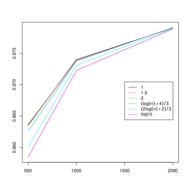
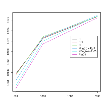
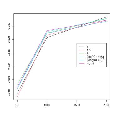
Figure 2: Out-of-sample AUC from fitting our model to simulations from Models 1 to 4 with $p=8$ covariates as a function of the size $n$ of the training set for different values of the threshold $\tau$. The values have been averaged over $100$ data sets.

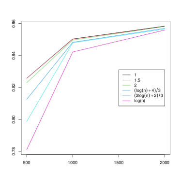
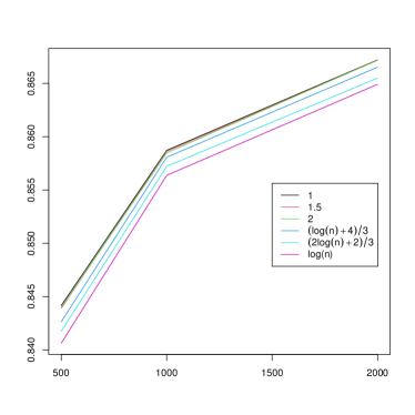
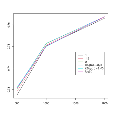
Figure 3: Out-of-sample AUC from fitting our model to simulations from Models 1 to 4 with $p=8$ covariates and weaker non-linearities and interaction effects as a function of the size $n$ of the training set for different values of the threshold $\tau$. The values have been averaged over $100$ data sets.

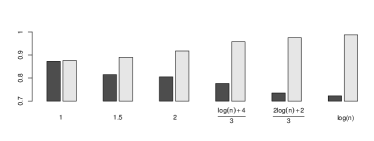
Figure 4: Fraction of true interactions that are found by our model (in dark gray) and of the selected interactions that are true interactions (in light gray) when fitting our model to simulations from Models 1 to 4 with $p=8$ and $n=500$ as a function of the $\tau$. The values have been averaged over $100$ data sets.

5.3 Comparison to other methods

As our model (denoted “Cop LR” in the tables below) is an extension of the simple logistic regression model with only linear main effects (denoted “Lin LR”), this is a natural reference, and thus one of the models we compare ours to. More specifically, we use the R package glm to fit such a model to all the simulated data sets. As mentioned earlier, our method may also be seen as an extension of a Naive Bayes model with specific marginal distributions. Therefore, we also include a Naive Bayes type model, namely one with normal margins (denoted “NB ”). We also tried such a model with kernel density estimators for the margins, but it gave either comparable or worse results than the one with normal margins, and the corresponding results are therefore not shown here. In the Naive Bayes model each margin is estimated separately with maximum likelihood, dividing the data according to class. This model can represent quadratic main effects, but not interaction effects. Finally, we include a logistic regression model with linear main effects and pairwise interactions (denoted “Int LR”), which is another way of extending the logistic regression model. This model is fitted using the method by Lim and Hastie [2015], which is based on grouped lasso, and is implemented in the R package glinternet. Here, we use 10-fold cross validation to find the optimal penalty, which is the default in glinternet.

The results in terms of the AUC for $p=8$ for the models with strong interactions and non-linearities are given in Table 1. The first thing we note is that the simple linear model performs very poorly. Further, the two Naive Bayes models give somewhat better results, but not nearly as good as the logistic regression model with pairwise interactions. This means that both non-linearities and interaction effects really are essential for discriminating between the two classes in this case. Further, we see that our method provides even better results than the logistic regression model with pairwise interactions, especially for data from Models 3 and 4, which contain more complex interaction effects, but also for Models 1 and 2, which only contain pairwise interactions. Results for the models with $p=14$ and $p=20$ covariates are quite similar, and are displayed in the supplementary material. So are the log-likelihoods which also follow the same patterns.

The results for the models with weaker interactions and non-linearities are given in Table 2. The simple linear model performs better in this case, which illustrates that the linear part of the main effects is relatively more important. Still, our method mostly gives better results than all the other methods and never worse, even for the smallest training set sizes. Hence, the non-linearities and interactions do not necessarily have to be that strong for our method to be useful.

Finally, since our model has potential to become quite complex, there may be a risk of over-fitting, especially if the true data generating mechanism is such that the corresponding discriminative model has log odds that are close to linear. In order to investigate this, we also simulated data from a model on the same form as Model 2, but with all correlations of $\mathbf{R}_{0}$ and $\mathbf{R}_{1}$ set to $0$, that we denote Model 5. The corresponding log odds of the corresponding discriminative model only has linear main effects and no interactions. The results from fitting our model and the competitors to data from this model with $p=8$ are given in Table 3. We see that even in this case the results from our method are comparable to the others. That being said, our model is much slower to fit than the others, and is mainly useful when there really are non-linearities and complex interactions in the data.

Sim. mod.	n	Cop LR	Lin LR	NB	Int LR
Model 1	$500$	0.963	0.501	0.627	0.933
	$1000$	0.974	0.501	0.639	0.939
	$2000$	0.979	0.501	0.644	0.943
Model 2	$500$	0.966	0.501	0.501	0.935
	$1000$	0.973	0.501	0.501	0.940
	$2000$	0.977	0.501	0.500	0.943
Model 3	$500$	0.936	0.501	0.622	0.688
	$1000$	0.939	0.501	0.635	0.716
	$2000$	0.941	0.501	0.641	0.730
Model 4	$500$	0.916	0.501	0.500	0.701
	$1000$	0.923	0.501	0.500	0.721
	$2000$	0.934	0.502	0.498	0.732

Table 1: AUC from fitting our model, as well as simple logisitic regression, Naive Bayes and logistic regression with pairwise interactions to simulations from Models 1 to 4 with $p=8$ covariates for different sizes $n$ of the training set. The values have been averaged over $100$ data sets.

Sim. mod.	n	Cop LR	Lin LR	NB	Int LR
Model 1	$500$	0.772	0.589	0.769	0.735
	$1000$	0.774	0.598	0.774	0.751
	$2000$	0.778	0.602	0.776	0.759
Model 2	$500$	0.823	0.574	0.534	0.695
	$1000$	0.850	0.582	0.544	0.712
	$2000$	0.858	0.587	0.551	0.720
Model 3	$500$	0.844	0.585	0.749	0.714
	$1000$	0.858	0.592	0.753	0.737
	$2000$	0.867	0.596	0.756	0.749
Model 4	$500$	0.730	0.623	0.558	0.667
	$1000$	0.751	0.630	0.567	0.688
	$2000$	0.764	0.633	0.572	0.699

Table 2: AUC from fitting our model, as well as simple logisitic regression, Naive Bayes and logistic regression with pairwise interactions to simulations from Models 1 to 4 with $p=8$ covariates and weaker non-linearities and interactions for different sizes $n$ of the training set. The values have been averaged over $100$ data sets.

n	Cop LR	Lin LR	NB	Int LR
$500$	0.939	0.942	0.942	0.940
$1000$	0.942	0.943	0.943	0.942
$2000$	0.943	0.944	0.944	0.943

Table 3: AUC from fitting our model, as well as simple logisitic regression, Naive Bayes and logistic regression with pairwise interactions to simulations from Model 5 with $p=8$ covariates for different sizes $n$ of the training set. The values have been averaged over $100$ data sets.

6 Real data examples

Next, we illustrate our method on a couple of real data sets, namely the ionosphere (Section 6.1) and the smoking data (Section 6.2).

6.1 Ionoshere data

First, we consider a dataset of radar returns that was discussed in a paper by Sigillito et al. [1989], where the objective is to classify observations as either ‘bad’ or ‘good’, so that bad returns may be removed automatically. The dataset contains $351$ observations of $34$ covariates, as well as the binary outcome variable, of which $126,$ roughly $36\%,$ have the value ‘bad’, and the rest are ‘good’. Two of the covariates are binary, but one of them only takes the value $0$, and the other is always $1$ when the outcome variable is ‘good’. Therefore, we choose to remove them from the dataset, leaving $32$ continuous covariates. We split the data into a training set of $263$ and a test set of $88$ observations, which corresponds to a $75/25\%$ split. Further, we let the outcome $y$ be $1$ if the observation is ‘bad’, and $0$ if it is ‘good’, and the balance between $0$s and $1$s is approximately the same in both the training and the test sets as in the full data set.

We fit our model, as well as the three competitor models from the simulation study. The corresponding results in term of the out-of-sample AUC and log-likelihood on the test set are given in the top two rows of Table 4. Our model provides by far the best results both in terms of the AUC and the log-likelihood. The improvement over the simple logistic regression with linear log-odds is huge, indicating that there are important non-linearities and/or interaction effects for explaining the response. The fact that both the Naive Bayes and the logistic regression with pairwise interactions also perform much better than the simple model, indicate that both non-linear main effects and interactions contribute.

Data set	Measure	Cop LR	Lin LR	NB	Int LR
Ionoshere data	AUC	0.957	0.766	0.926	0.890
	log-likelihood	-21.1	-93.7	-105.2	-95.7
Smoking data	AUC	0.839	0.831	0.792	0.837
	log-likelihood	-6476.0	-6548.1	-19856.7	-6484.6

Table 4: Out-of-sample AUC and log-likelihood from fitting our model (Cop LR), as well as simple logistic regression (Lin LR), Naive Bayes (NB) and logistic regression with pairwise interactions (Int LR), to the ionoshphere (top two rows) and the smoking data (bottom two rows).

6.2 Smoking data

Next, we look at the body signal of smoking data set from Kaggle [Bhargavi, 2022], that consists of $55962$ observations of the response, which is an indicator of whether the person is smoking or not, and $25$ covariates, describing a set of bio-indicators, such as age, height, weight, blood pressure and cholesterol. Out of these, $18$ are continuous. The covariate oral only takes one value, and is therefore removed. The remaining $6$ are categorical, more specifically binary, except Urine.protein, which takes $6$ categories. A preliminary analysis indicated that the categorical covariates eyesight.right and Urine.protein have little or no effect of the smoking status, and were therefore also removed, the former, probably because it almost always has the same value as eyesight.left, whereas very few observations were in categories $2$-$6$ for the latter. The remaining data consists of $18$ continuous covariates and $4$ binary ones, in addition to the response. Finally, we made a $75/25\%$ split of the data into a training set of $41769$ and a test set of $13923$.

The out-of sample AUC and log-likelihood from fitting the same models as to the ionosphere data are shown in the last two rows of Table 4. Our model gives the highest AUC and log-likelihood value, though very closely followed by the logistic regression model with pairwise interactions. The Naive Bayes model has the poorest relative performance, which may be due to the large sample size, as it tends to be comparatively better in relation to discriminative methods for smaller sample sizes [Ng and Jordan, 2002]. Further, there is some improvement from using the simple logistic regression model, but not nearly as large as for the ionosphere data. This means that the linear part of the log odds provides the largest part of the explanation of the response, but better predictions may be obtained by including interactions and non-linearities.

It should be noted that our fitted model includes seven copulas in the first tree of the vine copula and none in the following trees, resulting in $1+22+2\cdot 7=37$ parameters in total. This means that it contains seven pairwise interactions and none with higher order, more specifically between age and systolic (blood pressure), between eyesight.right and relaxation (blood pressure), between systolic and HDL (cholesterol type), between HDL and LDL (cholesterol type), between LDL and hemoglobin, between age and ALT (glutamic oxaloacetic transaminase type) and between weight.kg and serum.creatinine. On the other hand, the logistic regression with pairwise interactions includes all main effects (just like ours), in addition to $58$ interactions, $5$ of which were in common with our model, namely the first five listed above. This gives $1+22+58=81$ parameters, i.e. more than twice as many as our model. Hence, in this case, we obtain a much simpler model with at least as good performance.

7 Concluding remarks

We have proposed a generalisation of the simple logistic regression model that can account for non-linear main effects and complex interactions in the log odds, yet keeping the model based on an inherently interpretable structure. This model is constructed through a specification on generative form, with given marginal distributions from the natural exponential family, combined with vine copulas to describe the dependence. The model parameters are however estimated based on the discriminative likelihood function, and dependencies between covariates in the two classes are only included if they contribute significantly to the discrimination between the two classes. Further, we propose a scheme for doing model selection and estimation.

To assess the performance of our model, we have conducted a simulation study, which indicates that our model overall gives good results, also when the sample size is not very large compared to the number of covariates and in cases where non-linearities and interactions are not that strong. We also compared our model to alternative extensions of the simple logistic regression model, namely a Naive Bayes model and a logistic regression model with pairwise interactions. Our model performed either comparably to or better than the others, especially in cases with strong non-linearities and complex interactions. We also fitted our model to two real data sets, namely the ionosphere and the smoking data. Again, the results from our model were either similar to or better than the compared models. In particular, the model fitted to the smoking data was much simpler than the best competitor, i.e. the logistic regression with pairwise interactions, and yet performed just as well.

In the current version of the model selection and estimation procedure, we make an assumption of strong hierarchy for interactions of order three and higher. This means that such interactions are only considered for inclusion in the model if all sub interactions of lower order are already in the model. The reason for this assumption is computational, as it strongly reduces the number of interactions to check, and thus the computational burden. It is however straightforward to allow for a weak or no hierarchy instead. Further, our model is only composed of interactions between continuous covariates. There is however no explicit way to incorporate interactions between discrete covariates or between continuous and discrete ones, and this is a subject for further work.

8 Acknowledgements

This work is funded by The Research Council of Norway centre Big Insight, Project 237718.

References

- Aas et al. [2009] Aas, K., Czado, C., Frigessi, A., Bakken, H., 2009. Pair-copula constructions of multiple dependence. Insurance: Mathematics and economics 44, 182–198.
- Bedford and Cooke [2001] Bedford, T., Cooke, R.M., 2001. Probability density decomposition for conditionally dependent random variables modeled by vines. Annals of Mathematics and Artificial intelligence 32, 245–268.
- Bedford and Cooke [2002] Bedford, T., Cooke, R.M., 2002. Vines: A new graphical model for dependent random variables. Annals of Statistics , 1031–1068.
- Bhargavi [2022] Bhargavi, R., 2022. Smoking prediction. URL: https://kaggle.com/competitions/smoking-prediction.
- Bien et al. [2013] Bien, J., Taylor, J., Tibshirani, R., 2013. A lasso for hierarchical interactions. Annals of Statistics 41, 1111–1141.
- Brechmann et al. [2012] Brechmann, E., Czado, C., Aas, K., 2012. Truncated regular vines in high dimensions with application to financial data. Canadian Journal of Statistics 40, 68–85.
- Cox and Snell [1989] Cox, D., Snell, E., 1989. Analysis of binary data. Chapman & Hall.
- Czado [2019] Czado, C., 2019. Analyzing Dependent Data with Vine Copulas – A Practical Guide With R. volume 222. Springer.
- Efron [1975] Efron, B., 1975. The efficiency of logistic regression compared to normal discriminant analysis. Journal of the American Statistical Association 70, 892–898.
- Glad [2001] Glad, I., 2001. Parametrically guided nonparametric regression 25, 649–668.
- Goodman and Flaxman [2016] Goodman, B., Flaxman, S., 2016. Eu regulations on algorithmic decision-making and a “right to explanation”, in: ICML workshop on human interpretability in machine learning (WHI 2016), New York, NY. http://arxiv. org/abs/1606.08813 v1.
- Joe [1996] Joe, H., 1996. Families of m-variate distributions with given margins and m (m-1)/2 bivariate dependence parameters. Lecture Notes-Monograph Series , 120–141.
- Joe [1997] Joe, H., 1997. Multivariate Models and Dependence Concepts. Chapman Hall, London.
- Joe et al. [2010] Joe, H., Li, H., Nikoloulopoulos, A., 2010. Tail dependence functions and vine copulas. Journal of Multivariate Analysis 101, 252–270.
- Kurowicka and Cooke [2006a] Kurowicka, D., Cooke, R., 2006a. Uncertainty Analysis with High Dimensional Dependence Modelling. Wiley, New York.
- Kurowicka and Cooke [2006b] Kurowicka, D., Cooke, R., 2006b. Uncertainty Analysis with High Dimensional Dependence Modelling. Wiley, Chichester.
- Lim and Hastie [2015] Lim, M., Hastie, T., 2015. Learning interactions via hierarchical group-lasso regularization. Journal of Computational and Graphical Statistics 24, 627–654.
- Morris [1982] Morris, C.N., 1982. Natural exponential families with quadratic variance functions. The Annals of Statistics , 65–80.
- Nešlehová and Genest [2007] Nešlehová, J., Genest, C., 2007. A primer on copulas for count data. ASTIN bulletin 37, 475–515.
- Ng and Jordan [2002] Ng, A.Y., Jordan, M.I., 2002. On discriminative vs. generative classifiers: A comparison of logistic regression and naive bayes, pp. 841–848.
- O’Neill [1980] O’Neill, T., 1980. The general distribution of the error rate of a classification procedure with application to logistic regression discrimination. Journal of the American Statistical Association 75, 154–160.
- Panagiotelis et al. [2012] Panagiotelis, A., Czado, C., Joe, H., 2012. Pair copula constructions for multivariate discrete data. Journal of the American Statistical Association 107, 1063–1072.
- Panagiotelis et al. [2017] Panagiotelis, A., Czado, C., Joe, H., Stöber, J., 2017. Model selection for discrete regular vine copulas. Computational Statistics Data Analysis 106, 138–152.
- Rubinstein and Hastie [1997] Rubinstein, Y.D., Hastie, T., 1997. Discriminative vs informative learning., pp. 49–53.
- Rudin [2019] Rudin, C., 2019. Stop explaining black box machine learning models for high stakes decisions and use interpretable models instead. Nature machine intelligence 1, 206–215.
- Rudin et al. [2022] Rudin, C., Chen, C., Chen, Z., Huang, H., Semenova, L., Zhong, C., 2022. Interpretable machine learning: Fundamental principles and 10 grand challenges. Statistic Surveys 16, 1–85.
- Sigillito et al. [1989] Sigillito, V.G., Wing, S.P., Hutton, L.V., Baker, K.B., 1989. Classification of radar returns from the ionosphere using neural networks. Johns Hopkins APL Technical Digest 10, 262–266.
- Sklar [1959] Sklar, M., 1959. Fonctions de repartition an dimensions et leurs marges. Publ. inst. statist. univ. Paris 8, 229–231.
- Vogelaere [2020] Vogelaere, K., 2020. Using truncated vine copulas in Supervised Probabilistic Classification. Master’s thesis. Unviversité Catholique de Louvain.