Enumeration of planar bipartite tight irreducible maps

Abstract

We consider planar bipartite maps which are both tight, i.e. without vertices of degree $1$, and $2b$-irreducible, i.e. such that each cycle has length at least $2b$ and such that any cycle of length exactly $2b$ is the contour of a face. It was shown by Budd that the number $\mathcal{N}_{n}^{(b)}$ of such maps made out of a fixed set of $n$ faces with prescribed even degrees is a polynomial in both $b$ and the face degrees. In this paper, we give an explicit expression for $\mathcal{N}_{n}^{(b)}$ by a direct bijective approach based on the so-called slice decomposition. More precisely, we decompose any of the maps at hand into a collection of $2b$-irreducible tight slices and a suitable two-face map. We show how to bijectively encode each $2b$-irreducible slice via a $b$-decorated tree drawn on its derived map, and how to enumerate collections thereof. We then discuss the polynomial counting of two-face maps, and show how to combine it with the former enumeration to obtain $\mathcal{N}_{n}^{(b)}$.

1 Introduction

The study of random maps has been a subject of constant interest over the last sixty years, ever since Tutte’s first papers on the subject. Of particular interest is the number of maps of fixed genus $g$ and with $n$ labeled faces of prescribed degrees: explicit formulas were given by Tutte as early as 1961 in [Tut62] in the case of planar (i.e. genus $0$) maps with at most two faces of odd degree. This formula was extended very recently to the case of planar maps with an arbitrary (necessarily even) number of odd-degree faces in [BGM24a].

It was also recently realized that enumeration formulas remain simple in the case of tight maps, i.e. maps without vertices of degree $1$. It was shown by Norbury in [Nor10, Nor13] that the number of tight maps of fixed genus $g$ with $n$ labeled faces of respective degree $b_{1},\ldots,b_{n}$ is in fact a quasi-polynomial of degree $2n+6g-6$ in the $b_{i}$’s depending on their parity (provided that $n\geq 3$ if $g=0$). An explicit expression for this quasi-polynomial was given in [BGM24a] in the case $g=0$.

A remarkable extension of Norbury’s result was obtained by Budd in [Bud22] for the case of essentially $2b$-irreducible maps with even degrees $b_{i}=2m_{i}$. By essentially $2b$-irreducible, we mean maps that have no contractible cycle of length less than $2b$ and any contractible cycle of length $2b$ is the contour of a face of degree $2b$. It was shown that the number of such maps is now a polynomial of degree $2n+6g-6$ in both $b$ and the $m_{i}$’s. One of Budd’s motivations was to consider the limit where $b$ and the $m_{i}$’s are taken to be large, which corresponds to considering so-called irreducible metric maps, having an unexpected connection with Weil-Petersson volumes of hyperbolic surfaces [Bud22a].

The systematic study of planar irreducible maps, or more generally maps with a prescribed girth (which is the shortest length of a cycle in the map), was initiated by Bernardi and Fusy in [BF12, BF12a] via the existence of a canonical bi-orientation of such maps. In a later work, it was shown in [BG14, BG14a] how to recover their results by a substitution approach or, alternatively, via the decomposition of irreducible maps into slices upon cutting these maps along properly chosen geodesic paths. Let us also mention the paper [AP15] which develops an approach based on blossoming trees.

In [Bud22], Budd relies precisely on the substitution approach of [BG14] which, in the case of even-degree faces, he generalizes to maps having arbitrary genus and adapts to deal with tight maps. The purpose of the present paper is, in the case $g=0$, to recover and sharpen the results of [Bud22] by using instead the slice decomposition approach. This allows us to write a slightly more explicit expression for the polynomials counting $2b$-irreducible maps with prescribed even degrees, and to give a combinatorial interpretation of the various terms in that expression. Our main result consists in the following theorem:

Theorem 1.1.

Let $n,b,m_{1},\ldots,m_{n}$ be positive integers and let us denote by $\mathcal{N}_{n}^{(b)}(2m_{1},\allowbreak\ldots,2m_{n})$ the number of planar bipartite tight $2b$-irreducible maps with $n$ labeled faces of respective degrees $2m_{1},\ldots,2m_{n}$. Then, for $n\geq 3$, $m_{1}\geq b+1$ and $m_{2},\ldots,m_{n}\geq b$, we have

$$\mathcal{N}_{n}^{(b)}(2m_{1},\ldots,2m_{n})=(n-3)!\sum_{k_{1},\ldots,k_{n}\geq 0}p^{(b)}_{k_{1}}(m_{1})q^{(b)}_{k_{2}}(m_{2})\cdots q^{(b)}_{k_{n}}(m_{n})\alpha^{(b)}_{k_{1}+\cdots+k_{n},n-3}$$ (1)

where $p^{(b)}_{k}(m)$ and $q^{(b)}_{k}(m)$ denote the polynomials in $b$ and $m$:

$$p^{(b)}_{k}(m):=\binom{m-b-1}{k}\binom{m+b+k}{k}=\frac{1}{(k!)^{2}}\prod_{i=1}^{k}\left(m^{2}-(b+i)^{2}\right)$$ (2)

$$q^{(b)}_{k}(m):=\binom{m+b}{k}\binom{m-b-1+k}{k}=\frac{1}{(k!)^{2}}\prod_{i=0}^{k-1}\left(m^{2}-(b-i)^{2}\right)$$ (3)

and $\alpha^{(b)}_{k,n}$ the polynomial in $b$ given by the expression:

$$\alpha_{k,n}^{(b)}=[u^{n-k}]\frac{1}{\left(1-u\sum\limits_{j=2}^{b}\frac{1}{b}\binom{b}{j}\binom{b}{j-1}(-u)^{j-2}\right)^{n+1}}.$$ (4)

The quantity $\mathcal{N}_{n}^{(b)}(2m_{1},\ldots,2m_{n})$ is a polynomial in $b$ and $m_{1},\ldots,m_{n}$, of total degree $2n-6$. It is symmetric in the variables $m_{1},\ldots,m_{n}$, and even in each of them.

Some remarks are in order. First, note that $\alpha_{k,n}^{(b)}=0$ for $k>n$, hence the sum in (1) is a finite sum. Second, the fact that $\alpha_{k,n}^{(b)}$ is a polynomial in $b$ can be seen directly from (4) by noting that the fraction in the right-hand side is a series in $u$ whose coefficients are polynomial in $b$. We refer to Section 3.1 for a more detailed discussion, and in particular to Proposition 3.7 below for a manifestly polynomial expression of $\alpha_{k,n}^{(b)}$. Third, it follows from [BGM24a] that Theorem 1.1 also holds for $b=0$ upon understanding Equation (4) as $\alpha_{k,n}^{(0)}=\delta_{k,n}$ and noting that every map is $0$-irreducible. Finally, Equation (1) does not quite hold if we take all $m_{i}$ equal to $b$: for $n\geq 4$, one needs to add an extra pathological term $\frac{(n-1)!}{2}(-1)^{n}$, see [Bud22, Theorem 1] and Appendix C.

Outline.

Let us now discuss the path to Theorem 1.1. It is a consequence of a chain of bijective decompositions described in Section 2. The first idea, borrowed from [BGM24a], consists in decomposing a (at this stage, not necessarily irreducible nor tight) planar bipartite map into a two-face map with face degrees $2m_{1},2m_{2}$ and a collection of slices, which are so to say pieces of maps lying in-between two geodesics, built out of the faces with degrees $2m_{3},\ldots,2m_{n}$. This decomposition is recalled in Section 2.1, where we also show how to extend it to the case of tight irreducible maps by imposing simple conditions on the two-face map and independent irreducibility and tightness conditions on the slices. Then, following [BG14], we explain in Section 2.2 how a tight irreducible slice can be decomposed recursively. We show in Section 2.3 that this decomposition has a bijective representation involving a decorated tree which spans the derived map of the slice. A decorated tree is then naturally decomposed into its components living on the primal map, which we call arrow trees, and blossoming vertices which are isolated dual vertices with the same (prescribed) degrees as their corresponding primal faces, among $2m_{3},\ldots,2m_{n}$. Arrow trees and blossoming vertices are studied in Section 2.4. As seen in Section 2.5, the tightness property can be pulled back from the derived map onto the decorated tree, specifically as a property of its blossoming vertices.

Section 3 is devoted to the enumerative consequences of the above chain of decompositions. In practice, the initial problem of enumerating planar bipartite tight $2b$-irreducible maps with prescribed face degrees boils down to two separate counting problems. On the one hand, the problem of counting collections of tight irreducible slices; on the other hand, that of counting two-face maps. The first problem reduces to counting collections of decorated trees. This is performed in two steps. We first count arrow trees in Section 3.1 in two different ways, eventually yielding Equation (4) for their contribution $\alpha_{k,n}^{(b)}$ to formula (1), as well as a recursive way to compute it. We then evaluate in Section 3.2 the number of ways to connect the arrow trees via blossoming vertices into the desired collection of decorated trees. As it turns out, each individual configuration of a blossoming vertex is counted polynomially in $b$ and in the $m_{i}$ corresponding to its degree through Equation (3), and their connection with arrow trees amounts to a convolution which preserves this polynomiality. The second problem, i.e. counting two-face maps, is addressed in Section 3.3. The irreducibility constraint imposes that these two-face maps have a long enough cycle, which also yields a polynomial in $b,m_{1},m_{2}$ for their enumeration. Section 3.4 explains how to combine everything, namely how to attach the slices to the two-face maps. This last step leads to the formula (1), which is actually shown to be a totally symmetric polynomial in the $m_{i}$’s, which also depends polynomially on $b$. We also explore there a number of particular instances of Theorem 1.1.

Section 4 gathers some concluding remarks, while extra material may be found in the appendices. Appendix A discusses how to reconstruct a slice from its associated decorated tree, by a closing procedure. Appendix B checks the compatibility of formula (1) with the expression obtained in [Bud22]. Appendix C discusses the enumeration of $2b$-irreducible $2b$-angulations, which falls just outside the range of validity of Theorem 1.1.

Basic definitions.

Let us start by introducing some terminology related to maps, we refer to [Sch15] for more details. A planar map (hereafter called a map for short) is a connected (multi)graph drawn on the sphere without edge crossings. Loops and multiple edges are allowed. A map consists of vertices, edges and faces. It is customary to draw a planar map on the plane, this amounts to choosing one face as the outer face. A corner is the angular sector delimited by two consecutive edges incident to a same vertex, hence also incident to a same face. The degree of a vertex or a face is its number of incident corners. In this paper, we consider bipartite maps: the vertices can be partitioned in two sets in such a way that every edge connects vertices from different sets. Equivalently, for planar maps, this amounts to requiring that every face be of even degree.

A path on a map is a path on the sphere that consists of edges and vertices of the map. The length of a path is its number of edges, counted with multiplicity. The path is said simple if it does not visit a vertex more than once (except at its endpoints for a simple closed path). A simple closed path of non-zero length is called a cycle. The girth of a map is the minimal length of a cycle on the map. For $d$ a non-negative integer, a map is said $d$-irreducible if it has girth at least $d$, and every cycle of length $d$ is the contour of a face (by contour of a face, we mean the closed path formed by its incident edges). Note that every map is $0$-irreducible. As we consider bipartite maps, whose all cycles necessarily have even length, we will take $d$ an even integer and write $d=2b$.

Following [BGM24a], we define a tight map as a map with some of its vertices marked, which is such than any leaf (vertex of degree $1$) is marked. In particular, a tight map having no marked vertex is a map without leaves.

Given a map and two of its vertices $u,v$, the (graph) distance between $u$ and $v$ is the minimal length of a path connecting them. Such a path of minimal length is called a geodesic.

Acknowledgements.

We thank Timothy Budd, Guillaume Chapuy, Éric Fusy and Grégory Miermont for fruitful discussions related to this work. We acknowledge financial support from the Agence Nationale de la Recherche via the grants ANR-18-CE40-0033 “Dimers”, ANR-19-CE48-0011 “Combiné” and ANR-23-CE48-0018 “CartesEtPlus”.

2 Slice decomposition of (tight) irreducible maps

2.1 Slice decomposition of maps

An elementary slice is a planar map with one marked face, chosen as the outer face, having one marked incident vertex called the apex and one marked incident edge called the base, which satisfy the following constraints: denoting by $A$ the apex and by $B$, $C$ the endpoints of the base (with the outer face appearing on the right when going from $B$ to $C$),

• the blue boundary, defined as the portion $AB$ of the contour of the outer face when going from $A$ to $B$ with the outer face on the right is a geodesic,

• the red boundary, defined as the portion $CA$ of the contour of the outer face when going from $C$ to $A$ with the outer face on the right is the unique geodesic between $C$ and $A$,

• the apex is the only vertex common to the blue and red boundaries.

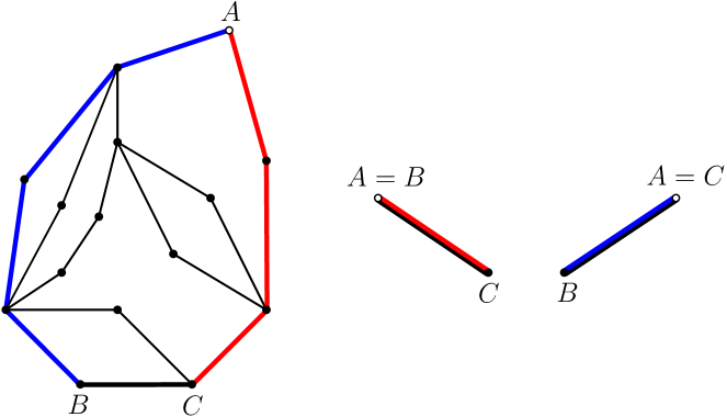
Figure 1: A generic slice (left) and the two possible slices without inner faces: the trivial slice (middle) and the empty slice (right).

See Figure 1 for examples. Note that, by the triangle inequality and the bipartiteness assumption, the length of $AB$ minus the length of $CA$ is equal to $\pm 1$. When this difference is equal to $-1$, then it follows from the above constraints that the whole slice is necessarily equal to the trivial slice, reduced to a single edge and two vertices, $A=B$ and $C$. In the following, we will call slice for short an elementary slice which is not trivial. Note that a slice may still be equal to the empty slice, reduced to a single edge and two vertices, $A=C$ and $B$. For $b$ a non-negative integer, we say that a slice is $2b$-irreducible if it has girth at least $2b$, and every cycle of length $2b$ is the contour of an inner face of the slice.

The following proposition is a slight variant of [BGM24a, Proposition 4.7]:

Proposition 2.1.

Fix an integer $n\geq 3$ and positive integers $m_{1},\ldots,m_{n}$. There is a bijection between the set of planar bipartite maps with $n$ labeled faces of respective degrees $2m_{1},\ldots,2m_{n}$, and the set of tuples of the form $(\mathbf{m}_{12},\mathbf{s}_{1},\ldots,\mathbf{s}_{k+1})$, for some $k$ between $0$ and $n-3$, such that:

• $\mathbf{m}_{12}$ is a planar map with exactly two (labeled) faces of respective degrees $2m_{1}$ and $2m_{2}$, and with $(k+1)$ among its vertices marked, one of them being distinguished,

• $\mathbf{s}_{i}$ is a non-empty slice for every $i=1,\ldots,k+1$,

• there is a bijection between $\{3,\ldots,n\}$ and the union of the sets of the inner faces of $\mathbf{s}_{1},\ldots,\mathbf{s}_{k+1}$, such that each $j=3,\ldots,n$ is mapped to a face of degree $2m_{j}$, and $3$ is mapped to an inner face of $\mathbf{s}_{1}$.

Remark 2.2.

A slight extension of this bijection applies to maps $\mathbf{m}$ which, in addition to the labeling of their faces, have some of their vertices marked (these can be intuitively regarded as “faces of zero degree”). Such maps still correspond to tuples $(\mathbf{m}_{12},\mathbf{s}_{1},\ldots,\mathbf{s}_{k+1})$ as above, but now each slice $\mathbf{s}_{i}$ may have some of its vertices not belonging to its red boundary marked, and may be reduced to the marked empty slice (i.e. the empty slice having its non-apex vertex marked). Under this bijection, the number of marked vertices in the original map is equal to the total number of marked vertices in $\mathbf{s}_{1},\ldots,\mathbf{s}_{k+1}$. In this paper, where we concentrate on irreducibility, we will always consider maps $\mathbf{m}$ without such faces of degree zero.

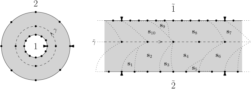
Figure 2: Sketch of the decomposition of a map $\mathbf{m}$ with two marked faces $1$ and $2$ (left) into elementary slices, by cutting its preimage $\tilde{\mathbf{m}}$ (right) along leftmost geodesics. In the notations of the main text, we have $m_{1}=6$, $m_{2}=4$ and $k=9$.

We refer to [BGM24a, Section 4.4] for a detailed description of the bijection. To summarize, it consists in the following steps, illustrated on Figure 2.

1. We start from a map $\mathbf{m}$ with $n$ labeled faces of respective degrees $2m_{1},\ldots,2m_{n}$ which we draw in the complex plane with the face $1$ containing the origin and the face $2$ chosen as the outer face. We call separating girth the minimal length of a separating cycle, i.e. a cycle enclosing the origin. We denote by $\gamma$ the innermost separating cycle of length equal to the separating girth. By convention we orient $\gamma$ in the counterclockwise direction.

2. We consider the preimage $\tilde{\mathbf{m}}$ of $\mathbf{m}$ by the mapping $z\mapsto\exp(2\mathrm{i}\pi z)$: it is an infinite map with two faces $\tilde{1}$ and $\tilde{2}$ of infinite degrees, which is invariant under the translation $z\mapsto z+1$. The minimal separating cycle $\gamma$ lifts to a biinfinite geodesic $\tilde{\gamma}=(\tilde{\gamma}_{i})_{i\in\mathbb{Z}}$, oriented from $-\infty$ to $+\infty$.

3. We cut $\tilde{\mathbf{m}}$ along each leftmost geodesic going from a corner incident to one of the infinite faces $\tilde{1}$ and $\tilde{2}$ to $\tilde{\gamma}_{i}$ for $i$ large enough (indeed such a leftmost geodesic eventually coalesces with $\tilde{\gamma}$). This decomposes $\tilde{\mathbf{m}}$ into a collection of elementary slices, possibly trivial or empty. Upon restricting to an appropriate fundamental domain, this collection is finite, and each face $3\ldots,n$ of $\mathbf{m}$ corresponds to an inner face of degree $2m_{i}$ appearing in exactly one slice. If the map $\mathbf{m}$ carries marked vertices, each of them appears in exactly one slice deprived of its red boundary, which allows to transfer the markings canonically.

4. We let $(\mathbf{s}_{1},\ldots,\mathbf{s}_{k+1})$ be the elementary slices in this decomposition which are neither trivial nor empty, where by convention $\mathbf{s}_{1}$ contains the face corresponding to face $3$, which allows us to list the other slices in some canonical way. Note that, since each of the $\mathbf{s}_{1},\ldots,\mathbf{s}_{k+1}$ contains at least a face, we have necessarily $k\leq n-3$.

5. By replacing the slices $(\mathbf{s}_{1},\ldots,\mathbf{s}_{k+1})$ by marked empty slices (i.e., empty slices with the non-apex vertex marked), and performing the slice decomposition backwards, we obtain the two-face map $\mathbf{m}_{12}$ with its $k+1$ marked vertices. The marked empty slice replacing $\mathbf{s}_{1}$ gives rise to the distinguished marked vertex in $\mathbf{m}_{12}$.

Let us record some useful properties of the above bijection in the following proposition, which combines the discussions of [BGM24a, Section 4.4] (regarding compatibility with tightness) and [BG14, Section 9.3] (regarding compatibility with irreducibility and girth constraints).

Proposition 2.3.

Let $\mathbf{m}$ be a planar map with $n$ labeled faces, let $(\mathbf{m}_{12},\mathbf{s}_{1},\ldots,\mathbf{s}_{k+1})$ be its image by the above bijection. Then:

• $\mathbf{m}$ is tight (i.e. has no leaves) if and only if all among $\mathbf{m}_{12},\mathbf{s}_{1},\ldots,\mathbf{s}_{k+1}$ are tight (note that $\mathbf{m}_{12}$ may have leaves provided they are marked),

• for any $b\geq 1$, $\mathbf{m}$ is essentially $2b$-irreducible (i.e. every non-separating cycle has length at least $2b$ and every such cycle of length $2b$ is the contour of a face) if and only if all among $\mathbf{s}_{1},\ldots,\mathbf{s}_{k+1}$ are $2b$-irreducible,

• the separating girth of the map $\mathbf{m}$ is equal to the length of the unique cycle of $\mathbf{m}_{12}$,

• the contour of face $2$ is the unique minimal separating cycle in $\mathbf{m}$ if and only if the corresponding second face in $\mathbf{m}_{12}$ is simple and has no incident marked vertex.

From these properties, denoting by $2m_{1}$ and $2m_{2}$ the degrees of faces $1$ and $2$, we deduce that, for any $b\geq 1$:

• if $m_{1},m_{2}>b$, $\mathbf{m}$ is $2b$-irreducible if and only if all among $\mathbf{s}_{1},\ldots,\mathbf{s}_{k+1}$ are $2b$-irreducible, and the length of the unique cycle of $\mathbf{m}_{12}$ is at least $2(b+1)$,

• if $m_{1}>b$, $m_{2}=b$, $\mathbf{m}$ is $2b$-irreducible if and only if all among $\mathbf{s}_{1},\ldots,\mathbf{s}_{k+1}$ are $2b$-irreducible, the length of the unique cycle of $\mathbf{m}_{12}$ is $2b$ (hence this cycle is the contour of face $2$), and none of the vertices of this cycle are marked.

In view of Propositions 2.1 and 2.3, the problem of enumerating planar bipartite tight $2b$-irreducible maps is highly dependent on our ability to characterize tight $2b$-irreducible slices. This is the purpose of the following sections where we show that $2b$-irreducible slices have a canonical decomposition which allows us to encode them by $b$-decorated plane trees, themselves formed of so-called $b$-arrow trees attached to each other via blossoming vertices.

Remark 2.4.

By specializing Propositions 2.1 and 2.3 to the case $m_{1}=b+1$ and $m_{2}=b$, we find that planar tight $2b$-irreducible maps with $n$ labeled faces of respective degrees $2b+2,2b,m_{3},\ldots,m_{n}$ are in bijection with tight $2b$-irreducible slices with $n-2$ labeled inner faces of respective degrees $m_{3},\ldots,m_{n}$. Indeed, we note that the map $\mathbf{m}_{12}$ produced in the decomposition consists of a cycle of length $2b$ to which is attached a single edge leading to a single marked vertex, which forces $k=0$ hence a single slice is obtained.

2.2 Recursive decomposition of irreducible slices

Let $b$ be a positive integer. As explained in details in [BG14], $2b$-irreducible slices can be decomposed recursively, at the price of introducing a slightly extended notion of slices. More precisely, for $p\geq 0$, we define a $2p$-slice as a planar map with one marked face (the outer face) having one marked incident vertex (the apex $A$) and one marked incident edge (the base $BC$) satisfying the following constraints:

• the blue boundary (defined as the portion $AB$ of the contour of the outer face when going from $A$ to $B$ with the outer face on the right) is a shortest path among all paths connecting $B$ to $A$ which do not pass via the base,

• the red boundary (portion $CA$ of the contour of the outer face when going from $C$ to $A$ with the outer face on the right) is the unique geodesic between $C$ and $A$,

• the apex is the only vertex common to the blue and red boundaries,

• the length of $AB$ minus the length of $CA$ is equal to $2p+1$,

• the slice has at least one inner face.

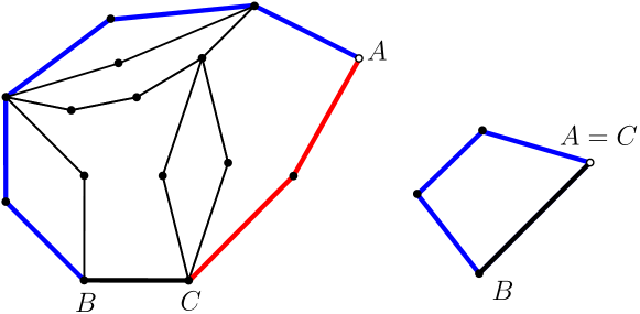
Figure 3: Examples of $2$-slices: a generic one (left)—note that it differs from the $0$-slice of Figure 1 only by a shift of the base edge—and the $4$-angle slice (right). Both are $4$-irreducible.

See Figure 3 for examples. Note that a $0$-slice is nothing but a non-trivial, non-empty elementary slice, and that the contour of the outer face of a $2p$-slice is simple. A $2p$-slice is said $2b$-irreducible if it has girth at least $2b$ and if every cycle of length $2b$ is the contour of an inner face.

We now discuss the precise recursive decomposition of a $2b$-irreducible $2p$-slice, for $p\leq b$ (we will not need the case $p>b$ in this paper). This requires us to distinguish three cases:

• when $0\leq p\leq b-1$, except special case (III) below;

• when $p=b$;

• when $p=b-1$ and the outer face has degree $2b$.

Recursive decomposition of a $\boldsymbol{2b}$-irreducible $\boldsymbol{2p}$-slice, case (I): $\boldsymbol{0\leq p\leq b-1}$.

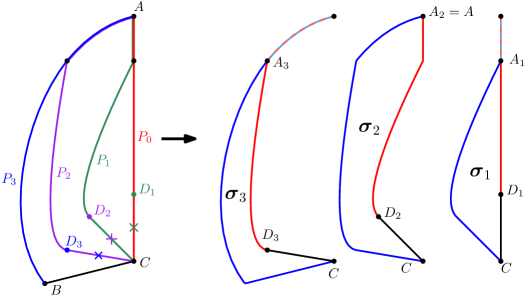
Figure 4: Case (I) of the decomposition. When $p\leq b-1$ and the slice is not reduced to the $2b$-angle slice, we know that $A\neq C$ so we name $D_{1}$ the first vertex on the red boundary $P_{0}$. $P_{1}$ is the leftmost shortest path from C to A avoiding $CD_{1}$. Cutting along $P_{1}$ yields a $2p_{1}$-slice $\boldsymbol{\sigma}_{1}$ with apex $A_{1}$ and base edge $CD_{1}$. We start again in the rest of the slice (which is now a $2(p-p_{1})$-slice with base $BC$), until $P_{q}$ goes through $BC$ and the blue boundary (here $q=3$).

Take a $2b$-irreducible $2p$-slice $\boldsymbol{\sigma}$, as defined just above, with $0\leq p\leq b-1$. The first step of the decomposition, illustrated on Figure 4, is done as follows: let us denote by $P_{0}$ the red boundary, travelled from $C$ to $A$, and by $P_{\infty}$ the longer path from $C$ to $A$ obtained by prefixing the blue boundary travelled from $B$ to $A$ with the base edge travelled from $C$ to $B$. The lengths of $P_{\infty}$ and $P_{0}$ differ by $2p+2$, and their sum is equal to the degree of the outer face. Using the $2b$-irreducibility constraint, we deduce that the length of $P_{0}$ cannot be equal to $0$ unless we have $p=b-1$ and the degree of the outer face is exactly $2b$: this case corresponds to a unique configuration, called the $2b$-angle slice, which will be treated separately in case (III) below. In all other cases, the length of $P_{0}$ is at least $1$, and we consider the leftmost shortest path $P_{1}$ among all paths from $C$ to $A$ which do not pass via the first edge $CD_{1}$ of $P_{0}$. Then, since $P_{0}$ is the unique geodesic from $C$ to $A$, the difference between the length of $P_{1}$ and that of $P_{0}$ must be positive, and is even by bipartiteness: it is equal to $2p_{1}$ for some $p_{1}\geq 1$. The part of $\boldsymbol{\sigma}$ in-between $P_{0}$ and $P_{1}$ is then a $2b$-irreducible $2p_{1}$-slice with base $CD_{1}$, which we denote by $\boldsymbol{\sigma}_{1}$. Note that we have $p_{1}\leq p+1$ since $P_{1}$ is not longer than $P_{\infty}$, and if $p_{1}=p+1$ then $P_{1}=P_{\infty}$: in this case, $\boldsymbol{\sigma}_{1}$ is the same map as $\boldsymbol{\sigma}$, except that we have shifted the base edge by one step to the right, so it becomes a $2(p+1)$-slice. For $p_{1}\leq p$, we continue the decomposition iteratively: denoting by $D_{2}$ the endpoint of the first edge of $P_{1}$, we consider the leftmost shortest path $P_{2}$ among all paths from $C$ to $A$ which stay in-between $P_{1}$ and $P_{\infty}$ and do not pass via the edge $CD_{2}$. Then, the length of $P_{2}$ is equal to that of $P_{1}$ plus $2p_{2}$ for some $p_{2}\geq 1$, and the part of the map in-between $P_{1}$ and $P_{2}$ is a $2b$-irreducible $2p_{2}$-slice with base $CD_{2}$, which we denote by $\boldsymbol{\sigma}_{2}$. As $P_{2}$ is not longer than $P_{\infty}$, we have $p_{1}+p_{2}\leq p+1$, and in the case of equality we have $P_{2}=P_{\infty}$, and we may stop the iteration. For $p_{1}+p_{2}\leq p$, we continue the iteration, defining a path $P_{3}$ and a $2p_{3}$-slice $\boldsymbol{\sigma}_{3}$ with $p_{3}\geq 1$ and $p_{1}+p_{2}+p_{3}\leq p+1$, and so on. Eventually, after $q$ iterations, we will have $P_{q}=P_{\infty}$, and $p_{1}+\cdots+p_{q}=p+1$, and we stop here. What we have done so far can be summarized into the following:

Proposition 2.5.

For any integers $b,p$ with $0\leq p\leq b-1$, there is a face-preserving bijection between the set of $2b$-irreducible $2p$-slices $\boldsymbol{\sigma}$ not equal to the $2b$-angle slice, and the set of sequences of the form $(\boldsymbol{\sigma}_{1},\ldots,\boldsymbol{\sigma}_{q})$ where $q$ is a positive integer and, for any $j=1,\ldots,q$, $\boldsymbol{\sigma}_{j}$ is a $2b$-irreducible $2p_{j}$-slice for some $p_{j}\geq 1$, with $p_{1}+\cdots+p_{q}=p+1$.

The bijectivity can be checked by exhibiting the reverse bijection: given a sequence $(\boldsymbol{\sigma}_{1},\ldots,\boldsymbol{\sigma}_{q})$ as in the proposition, it consists in gluing its elements into a single $2p$-slice $\boldsymbol{\sigma}$. The key property is that $2b$-irreducibility is preserved in this operation: in a nutshell this is because we are gluing along geodesics, hence we cannot create “short” cycles. See [BG14, Section 5.1].

We then continue the recursion by further decomposing the $\boldsymbol{\sigma}_{j}$. Two situations may occur:

• if $q\geq 2$, or if $p<b-1$, then each $\boldsymbol{\sigma}_{j}$ is a $2p_{j}$-slice with $p_{j}\leq b-1$: we may apply to it again the case (I) of the decomposition we have just described, or possibly the case (III) described below,

• otherwise, for $q=1$ and $p=b-1$, we get a single $2b$-slice $\boldsymbol{\sigma}_{1}$: we apply to it the case (II) of the decomposition described below.

Let us observe that, in each “branch” of the recursion, we will eventually arrive at either case (II) or case (III). Indeed, for $q>2$, each $\boldsymbol{\sigma}_{j}$ contains fewer faces than $\boldsymbol{\sigma}$ while, for $q=1$, we pass from a $2p$-slice to a $2(p+1)$-slice. So, we end up with either the $2b$-angle slice or a $2b$-irreducible $2b$-slice.

Remark 2.6.

This decomposition holds in particular for $p=0$, i.e. for non-empty $2b$-irreducible slices. In this case, we have necessarily $q=1$ and $p_{1}=1$. This corresponds to transforming the $0$-slice into a $2$-slice by changing its base from $BC$ to $CD_{1}$. For instance, applying the decomposition to the $0$-slice of Figure 1-left, we obtain the $2$-slice of Figure 3-left, where $CD_{1}$ is renamed $BC$.

Recursive decomposition of a $\boldsymbol{2b}$-irreducible $\boldsymbol{2p}$-slice, case (II): $\boldsymbol{p=b}$.

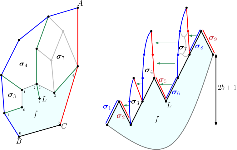
Figure 5: Case (II) of the decomposition, here for $p=b=1$. This 2-irreducible 2-slice is composed of a face $f$ of degree $10$, and $9$ elementary slices. Left: we draw the (green) leftmost geodesic towards the apex from each vertex incident to $f$; this delimits the slices $\boldsymbol{\sigma}_{1},\ldots,\boldsymbol{\sigma}_{9}$ (here, the slices $\boldsymbol{\sigma}_{1},\boldsymbol{\sigma}_{6}$ and $\boldsymbol{\sigma}_{8}$ are empty, and $\boldsymbol{\sigma}_{2},\boldsymbol{\sigma}_{5}$ and $\boldsymbol{\sigma}_{9}$ are trivial). The small labels in the corners of $f$ are the proximities to the apex, here equal to $5$ minus the length of a shortest path to $A$ avoiding $BC$: they go from $0$ at $B$ to $2b+1=3$ at $C$ by steps of $\pm 1$. Right: the result after cutting along the geodesics. The green arrows show how to glue back the elementary slice boundaries, in order to recover the original slice. Note that this slice is not tight, since it has a leaf $L$ incident to $f$.

Suppose now that we have a $2b$-irreducible $2b$-slice $\boldsymbol{\sigma}$ with apex $A$ and base $BC$, and consider the inner face $f$ immediately to the left of the base. Denoting by $2m$ the degree of $f$, consider its sequence of incident corners $(c_{0},\ldots c_{2m-1})$, as read clockwise around $f$ when going from $B$ to $C$, and introduce the proximity to the apex $\ell_{j}:=d(A,B)-d(A,V_{j})$, where $d(\cdot,\cdot)$ is the graph distance in $\boldsymbol{\sigma}$ deprived of its base edge, and $V_{j}$ is the vertex incident to $c_{j}$ for $j=0,\ldots,2m-1$. See Figure 5 for an example. We have in particular $\ell_{0}=0$ (since $V_{0}=B$), $\ell_{2m-1}=2b+1$ (by the definition of a $2b$-slice), and $|\ell_{j}-\ell_{j-1}|=1$ for any $j=1,\ldots,2m-1$. Note that this implies $m\geq b+1$. We may now cut the slice along the leftmost geodesic from $V_{j}$ to $A$, for all $j$. It is easily seen that the part of the map in-between the leftmost geodesic from $V_{j-1}$ to $A$ and the leftmost geodesic from $V_{j}$ to $A$ is a $2b$-irreducible elementary slice $\boldsymbol{\sigma}_{j}$ with base $V_{j-1}V_{j}$ for all $j\in\{1,\ldots,2m-1\}$. More precisely, $\boldsymbol{\sigma}_{j}$ is the trivial slice whenever $\ell_{j}-\ell_{j-1}=-1$ (this occurs $m-b-1$ times), while it is the empty slice or a $2b$-irreducible $0$-slice whenever $\ell_{j}-\ell_{j-1}=1$ (this occurs $m+b$ times). To summarize, we have the following:

Proposition 2.7.

For any integers $m>b\geq 1$, there is a quasi-face-preserving bijection between the set of $2b$-irreducible $2b$-slices where the base edge is incident to an inner face of degree $2m$, and the set of $(2m-1)$-tuples of $2b$-irreducible elementary slices, exactly $m-b-1$ of which being equal to the trivial elementary slice. (Note that the $m+b$ remaining elementary slices are necessarily either equal to the empty slice, or to a $2b$-irreducible $0$-slice.)

Again, the bijectivity can be checked by exhibiting the reverse bijection. The most subtle point, already discussed in [BG14], is to check that this reverse bijection preserves $2b$-irreducibility: again we use the fact that we are gluing slices along geodesics, but we must also observe that, when “recreating” the base edge $BC$, we connect two vertices at graph distance at least $2b+1$, so we cannot create a non-facial cycle of length $2b$. This property would not be ensured if we applied decomposition (II) to a $2p$-slice with $p<b$, and in particular to a $0$-slice. In retrospect, this justifies why we need to introduce $2p$-slices for $p>0$.

Having decomposed the $2b$-slice $\boldsymbol{\sigma}$ as above, two situations may occur:

• we only obtain trivial and empty slices: the recursive decomposition terminates here,

• we obtain at least one $0$-slice: we apply to it the case (I) of the decomposition, or possibly the special case (III) if $b=1$ and the $0$-slice is a $2$-angle.

Recursive decomposition of a $\boldsymbol{2b}$-irreducible $\boldsymbol{2p}$-slice, case (III): the $\boldsymbol{2b}$-angle slice.

We finally treat the special case where $p=b-1$ and the outer face is of degree $2b$. Since the contour of the outer face is a cycle, by irreducibility it is also the contour of an inner face $f$ of degree $2b$. The whole slice then consists of a single cycle of length $2b$. Note that, with $p=b-1$, the red boundary is reduced to the vertex $C=A$, and the blue boundary comprises all edges apart from the base. We call this slice the $2b$-angle slice. Such slice will be an atom in our recursive decomposition, which terminates here.

Altogether, combining steps (I), (II) and (III) decomposes any $2b$-irreducible $2p$-slice with $0\leq p\leq b$ into pieces which are either the trivial slice, the empty slice, or the $2b$-angle slice (one may check that the recursion always terminates by induction on the number of inner faces). Figure 6 shows an example of full decomposition of a $0$-slice in the case $b=2$.

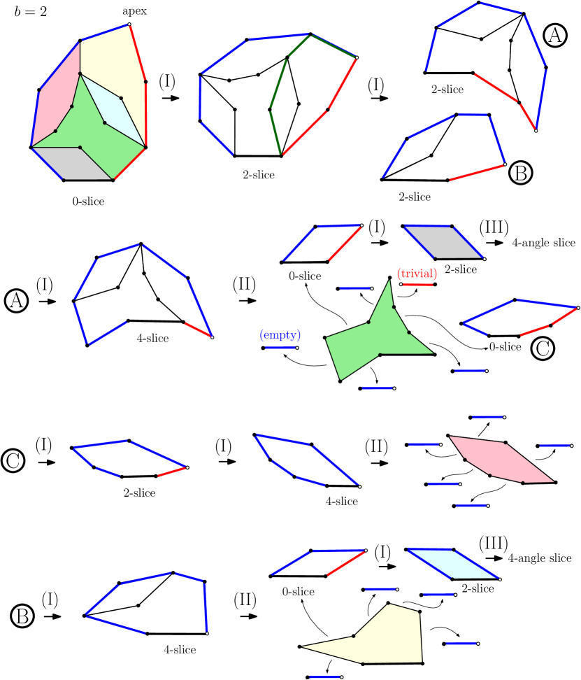
Figure 6: An example of decomposition of a $2b$-irreducible $0$-slice with $5$ faces, in the case $b=2$. In the second step (I) (upper line), the green geodesic cuts the $2$-slice in two sub-slices denoted by \raise-1pt\hbox{A}⃝ and \raise-1pt\hbox{B}⃝. In the end, we are left with $1$ occurrence of the trivial slice, $13$ occurrences of the empty slice, and $2$ occurrences of the $2b$-angle slice.

2.3 Decorated tree formulation

Assume $b>0$ and $0\leq p\leq b$ and consider a $2b$-irreducible $2p$-slice $\boldsymbol{\sigma}$ to which we apply the above recursive decomposition. Following [BG14, BG14a], it is useful to encode this decomposition in the form of a tree, which we call $b$-decorated tree or decorated tree for short, and we will denote by $T(\boldsymbol{\sigma})$. It turns out that $T(\boldsymbol{\sigma})$ can be naturally drawn on the derived map $\Delta(\boldsymbol{\sigma})$.

Recall from [Sch15] that the derived map $\Delta(M)$ of a map $M$ is the quadrangulation obtained by superimposing $M$—hereafter called the primal map—with its dual map. The derived map has three types of vertices, namely primal vertices, dual vertices and edge-vertices, which are respectively in bijection with the vertices, faces and edges of the primal map. Precisely, if the primal map has two vertices $U$ and $V$ connected by the edge $UV$ which has face $f$ on its left and face $g$ on its right, then the derived map has an edge-vertex $\Delta(UV)$ corresponding to the edge $UV$, which is of degree $4$ and connected (in clockwise order) to the vertices $\Delta(U),\Delta(f),\Delta(V),\Delta(g)$. Each edge of the derived map connects an edge-vertex to either a primal or a dual vertex, and hence corresponds to either a primal half-edge or a dual half-edge accordingly.

In addition to being drawn on the derived map, the tree $T(\boldsymbol{\sigma})$ carries some extra data, which we represent in the form of decorations as follows.

• Each primal half-edge belonging to $T(\boldsymbol{\sigma})$ and incident to a primal vertex of degree at least two in $T(\boldsymbol{\sigma})$ carries a number, ranging between $1$ and $b$, of arrows pointing from the primal vertex to the edge-vertex.

• Each dual vertex in $T(\boldsymbol{\sigma})$ may be incident, in addition to regular dual half-edges (which carry no arrow), to dangling half-edges which we call leaflets.

The reader is invited to have a first look at Figure 10, which features these decorations in the case $b=2$.

Let us now explain how to construct $T(\boldsymbol{\sigma})$. In a nutshell, we perform the recursive decomposition described in the previous subsection, and build progressively the tree at each step, according to specific rules described below. We start with the following useful definition:

Definition 2.8.

Given a $2p$-slice $\boldsymbol{\sigma}$, with apex $A$, base $BC$, and outer face $f_{0}$, we define the tree vertex set $S(\boldsymbol{\sigma})$ as the set of all vertices of the derived map $\Delta(\boldsymbol{\sigma})$ deprived of $\Delta(f_{0})$ and from the primal and edge-vertices corresponding to the vertices and edges of the blue boundary. In particular, neither $\Delta(A)$ nor $\Delta(B)$ belong to $S(\boldsymbol{\sigma})$, but $\Delta(BC)$ and $\Delta(f)$ do, where $f$ is the inner face incident to $BC$. We extend this definition by setting $S(\boldsymbol{\sigma})=\{\Delta(BC),\Delta(C)\}$ for $\boldsymbol{\sigma}$ the trivial slice, and $S(\boldsymbol{\sigma})=\varnothing$ for $\boldsymbol{\sigma}$ the empty slice.

This allows us to state an “invariant” of the recursion, which will be verified inductively:

Proposition 2.9.

Given a $2b$-irreducible $2p$-slice $\boldsymbol{\sigma}$ with $0\leq p\leq b$, $T(\boldsymbol{\sigma})$ is a tree drawn on the derived map $\Delta(\boldsymbol{\sigma})$, having vertex set $S(\boldsymbol{\sigma})$. Every edge-vertex in $S(\boldsymbol{\sigma})$ has degree two in $T(\boldsymbol{\sigma})$, except $\Delta(BC)$ which has degree one, and which we choose as the root. For $p=b$, $\Delta(BC)$ is connected to $\Delta(f)$. For $p\leq b-1$, $\Delta(BC)$ is connected to $\Delta(C)$ by a primal half-edge carrying $b-p$ arrows, unless $\boldsymbol{\sigma}$ is equal to the $2b$-angle slice, in which case $\Delta(BC)$ is connected to $\Delta(f)$.

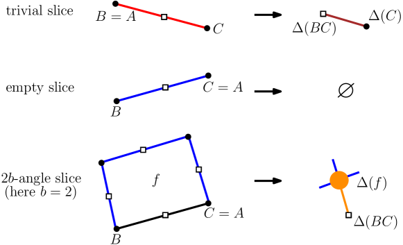
Figure 7: Initialisation of the recursive construction of $T(\boldsymbol{\sigma})$. Primal vertices and edge-vertices are represented as black dots and white squares, respectively. On the right, leaflets are shown in blue.

We now give the precise construction rules. See Figure 10 for a full application of our construction.

Recursive construction of the decorated tree, initialisation.

We define $T(\boldsymbol{\sigma})$ when $\boldsymbol{\sigma}$ is an “atom” of our recursive decomposition, namely when it is equal either to the trivial slice, to the empty slice, or to the $2b$-angle slice. For the trivial slice, $T(\boldsymbol{\sigma})$ consists of a single primal half-edge connecting $\Delta(BC)$ to $\Delta(C)$, carrying no arrow. This tree is called the trivial tree. For the empty slice, $T(\boldsymbol{\sigma})$ is defined as the empty graph containing no vertex. For the $2b$-angle slice, corresponding to the case (III) discussed in the previous subsection, $T(\boldsymbol{\sigma})$ consists of a single dual half-edge connecting $\Delta(BC)$ to $\Delta(f)$ (with $f$ the inner face), and $2b-1$ leaflets incident to $\Delta(f)$. See Figure 7 for an illustration. Note that all these conventional definitions are consistent with the property that $T(\boldsymbol{\sigma})$ has vertex set $S(\boldsymbol{\sigma})$. We now turn to the recursive part of the construction, for which we have to distinguish the cases (I) and (II) discussed in the previous subsection.

Recursive construction of the decorated tree, case (I): $\boldsymbol{0\leq p\leq b-1}$.

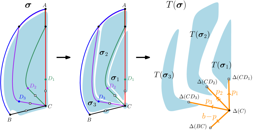
Figure 8: Tree formulation of the case (I) decomposition of Figure 4. Primal vertices and edge-vertices are represented as black dots and white squares, respectively. Represented in light blue, the tree vertex set $S(\boldsymbol{\sigma})$ (left), and its decomposition as the disjoint union of the sets $\{\Delta(BC)\},\{\Delta(C)\},S(\boldsymbol{\sigma}_{1}),\ldots,S(\boldsymbol{\sigma}_{q})$ (middle). On the right, the tree $T(\boldsymbol{\sigma})$ constructed in the text.

Suppose that we are in case (I) of the recursive decomposition. As summarized in Proposition 2.5, $\boldsymbol{\sigma}$ is then decomposed into a sequence $(\boldsymbol{\sigma}_{1},\ldots,\boldsymbol{\sigma}_{q})$ where $q$ is a positive integer and, for any $j=1,\ldots,q$, $\boldsymbol{\sigma}_{j}$ is a $2b$-irreducible $2p_{j}$-slice for some $p_{j}\geq 1$, with $p_{1}+\cdots+p_{q}=p+1$. Then, $T(\boldsymbol{\sigma})$ consists of the following elements (see Figure 8 for an illustration):

• the primal half-edge connecting $\Delta(BC)$ to $\Delta(C)$, on which we place $b-p$ arrows,

• for each $j=1,\ldots,q$, the primal half-edge connecting $\Delta(C)$ to $\Delta(CD_{j})$ (with $CD_{j}$ the base of $\boldsymbol{\sigma}_{j}$), on which we place $p_{i}$ arrows,

• and the trees $T(\boldsymbol{\sigma}_{1}),\ldots,T(\boldsymbol{\sigma}_{q})$ which we proceed to construct recursively.

Assuming that Proposition 2.9 holds for $\boldsymbol{\sigma}_{1},\ldots,\boldsymbol{\sigma}_{q}$, we may verify that it also holds for $\boldsymbol{\sigma}$, by making the key observation that the tree vertex set $S(\boldsymbol{\sigma})$ is the disjoint union of the sets $\{\Delta(BC)\},\{\Delta(C)\},S(\boldsymbol{\sigma}_{1}),\ldots,S(\boldsymbol{\sigma}_{q})$. We also observe that, in $T(\boldsymbol{\sigma})$, the primal vertex $\Delta(C)$ has degree $q+1\geq 2$, and that the total number of arrows on its incident primal half-edges is equal to $(b-p)+p_{1}+\cdots+p_{q}=b+1$.

Recursive construction of the decorated tree, case (II): $\boldsymbol{p=b}$.

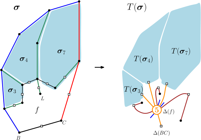
Figure 9: Tree formulation of the case (II) decomposition of Figure 5 (for $b=1$). In $T(\boldsymbol{\sigma})$, the empty slices $\boldsymbol{\sigma}_{1},\boldsymbol{\sigma}_{6},\boldsymbol{\sigma}_{8}$ give rise to leaflets (shown in blue) while the trivial slices $\boldsymbol{\sigma}_{2},\boldsymbol{\sigma}_{5},\boldsymbol{\sigma}_{9}$ give rise to twigs (shown in brown). For convenience we display on the dual vertex $\Delta(f)$ its half-degree, here equal to $m=5$. Note that the vertex $L$ of degree $1$ incident to $f$ in $\boldsymbol{\sigma}$ gives rise in $T(\boldsymbol{\sigma})$ to a twig followed by a leaflet, when going clockwise around $\Delta(f)$. Such pattern is forbidden in tight maps.

Suppose now that we are in case (II) of the recursive decomposition and let $m$ be the half-degree of the inner face $f$. As summarized in Proposition 2.7, $\boldsymbol{\sigma}$ is then decomposed into a tuple $(\boldsymbol{\sigma}_{1},\ldots,\boldsymbol{\sigma}_{2m-1})$ of $2b$-irreducible elementary slices, exactly $m-b-1$ of which are trivial. Then, $T(\boldsymbol{\sigma})$ consists of the following elements (see Figure 9 for an illustration):

• the dual half-edge connecting $\Delta(BC)$ to $\Delta(f)$,

• for each $j=1,\ldots,2m-1$, the dual half-edge connecting $\Delta(f)$ to the edge-vertex corresponding to the base of $\boldsymbol{\sigma}_{j}$, unless the latter is equal to the empty slice, in which case we replace the dual half-edge by a leaflet attached to $\Delta(f)$,

• and the trees $T(\boldsymbol{\sigma}_{1}),\ldots,T(\boldsymbol{\sigma}_{2m-1})$ which we proceed to construct recursively.

Assuming that Proposition 2.9 holds for the $\boldsymbol{\sigma}_{j}$ which are neither trivial nor empty, we may verify that it also holds for $\boldsymbol{\sigma}$, by making the key observation that the tree vertex set $S(\boldsymbol{\sigma})$ is the disjoint union of the sets $\{\Delta(BC),\Delta(f)\},S(\boldsymbol{\sigma}_{1}),\ldots,S(\boldsymbol{\sigma}_{2m-1})$. We also observe that, in $T(\boldsymbol{\sigma})$, the dual vertex $\Delta(f)$ has degree $2m$, accounting for the contribution of leaflets. It is incident to exactly $m-b-1$ dual half-edges leading to an instance of the trivial tree (namely, the tree corresponding to the trivial slice, see again Figure 7). We call twig the combination of such a dual half-edge and its attached trivial tree, so that $\Delta(f)$ is attached to exactly $m-b-1$ twigs. The remaining contribution $m+b+1$ to the degree of $\Delta(f)$ comes from leaflets, dual half-edges leading to non-trivial trees, and the root dual half-edge coming from $\Delta(BC)$.

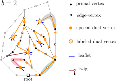
Figure 10: The decorated tree representation of the decomposition in Figure 6. Here we draw the tree superimposed on the slice. We indicated in light blue a bioriented edge-vertex, in gray a regular bent edge-vertex, and in pink a special bent edge-vertex. The primal and edge-vertices corresponding to the blue boundary of the slice are shown in grey, and do not belong to the tree vertex set.

Characterization of $b$-decorated trees.

Let us now give an intrinsic characterization of the trees that we obtain. A $b$-decorated tree is a plane tree satisfying the following properties.

• It is made of three types of vertices: primal, dual, and edge-vertices, connected by either primal half-edges connecting a primal vertex to an edge-vertex, or dual half-edges connecting a dual vertex to an edge-vertex.

• It carries two types of decorations:

  • arrows, in number between $1$ and $b$, placed on all primal half-edges incident to a primal vertex of degree at least two, and pointing away from that vertex;

  • leaflets, incident to dual vertices, that contribute to their degrees.

• Around each primal vertex of degree at least two, the total number of arrows is equal to $b+1$.

• The tree is planted on an edge-vertex of degree one, hereafter called the root. All the edge-vertices different from the root have degree two.

• An edge-vertex incident to two primal half-edges is called a bioriented edge: it must have both its incident half-edges carrying arrows, with $b$ arrows in total, and may therefore exist only when $b\geq 2$.

• An edge-vertex incident to two dual half-edges is called a dual/dual edge-vertex: it may exist only when $b=1$, and must have exactly one of its adjacent dual vertices of degree $2b=2$ (see Figure 14).

• An edge-vertex incident to one primal half-edge and one dual half-edge is called a bent edge-vertex, which must be of one of the following types:

  • a twig-vertex: the primal half-edge carries no arrow, hence leads to a primal vertex of degree one. The ensemble made of the twig-vertex, its incident half-edges, and the adjacent primal vertex, form a twig;

  • a special bent edge-vertex: the primal half-edge carries $b-1$ arrows, and the adjacent dual vertex has degree $2b$;

  • a regular bent edge-vertex: the primal half-edge carries $b$ arrows, and the adjacent dual vertex has degree at least $2b+2$.

• Each dual vertex of degree $2b$, hereafter called special dual vertex, is incident to exactly one dual half-edge and $2b-1$ leaflets.

• Every other dual vertex has an even degree larger than $2b$, and is hereafter called labeled dual vertex. A labeled dual vertex of degree $2m$ has label $m\geq b+1$, and is adjacent to exactly $m-b-1$ twig-vertices.

See again Figure 10 for an example of a $b$-decorated tree in the case $b=2$. With this characterization at hand, we may state the following:

Proposition 2.10.

For $b\geq 1$ and $p=0,\ldots,b$, the mapping $\boldsymbol{\sigma}\mapsto T(\boldsymbol{\sigma})$ is a bijection between the set of $2b$-irreducible $2p$-slices different from the $2b$-angle slice, and the set of $b$-decorated trees such that the root edge-vertex is incident to a primal half-edge carrying $b-p$ arrows when $p\leq b-1$, or to a dual half-edge leading to a labeled dual vertex when $p=b$. For each $m$, the number of inner faces of degree $2m$ in $\boldsymbol{\sigma}$ is equal to the number of dual vertices of degree $2m$ in $T(\boldsymbol{\sigma})$.

This proposition may be proved by checking that the $b$-decorated trees have a recursive decomposition which is equivalent to that of $2b$-irreducible slices. For completeness, we also give a self-contained description of the inverse bijection in Appendix A.

Remark 2.11.

For completeness, let us mention an alternate but equivalent way to represent $b$-decorated trees, which is strongly reminiscent of the $\mathbb{Z}$-mobiles considered in [BF12a]. We still have three types of vertices (primal, dual and edge-vertices), connected by primal and dual half-edges. We still plant the tree on an edge-vertex of degree one, and every other edge-vertex has degree two. We still have leaflets attached to the dual vertices and contributing to their degree (which must be an even integer larger than or equal to $2b$). But instead of placing arrows on some primal half-edges, we now assign an integer weight to every (primal or dual) half-edge, with the following rules:

• the weight of a primal half-edge is an integer between $1$ and $b+1$,

• the weight of a dual half-edge is either $-1$, $0$ or $+1$,

• defining the total weight of a vertex as the sum of the weights of its incident half-edges (ignoring leaflets):

  • each primal vertex has total weight $b+1$,

  • each non-root edge-vertex has total weight $b$,

  • for every $m\geq b$, each dual vertex of degree $2m$ has total weight $b+1-m$; if $m=b$ it is incident to exactly one dual half-edge of weight $+1$ and $2b-1$ leaflets; if $m\geq b+1$ it has no incident dual half-edge of weight $+1$ (hence has exactly $m-b-1$ incident dual half-edges of weight $-1$).

We recover the previous representation by placing $i$ arrows on each primal half-edge of weight $i$, for every $i$ between $1$ and $b$. Note that the primal half-edges of weight $b+1$ and the dual half-edges of weight $-1$ only appear within twigs. Let us observe finally that, in the absence of dual vertices of degree $2b$ (which implies that there are no dual half-edges of weight $+1$), we recover precisely the $(b+1)$-dibranching mobiles as defined in [BF12a, Definition 8].

2.4 Arrow trees and blossoming vertices.

From the discussion of the previous subsections, the problem of enumerating $2b$-irreducible maps can be achieved by first enumerating $2b$-irreducible slices, which in turn amounts to enumerating $b$-decorated trees. In order to do so, it is useful to further decompose these decorated trees into more elementary components as follows (see Figure 11).

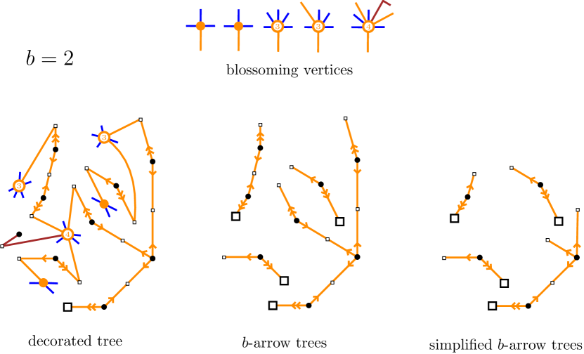
Figure 11: Decomposition of the decorated tree (left) of Figure 10 into its connected components made of $b$-arrow trees and blossoming vertices (middle). The $b$-arrow trees may be further reduced into simplified $b$-arrow trees (right).

Let us assume first that $b>1$ (the case $b=1$ will be treated at the end of this subsection).

$\boldsymbol{b}$-arrow trees.

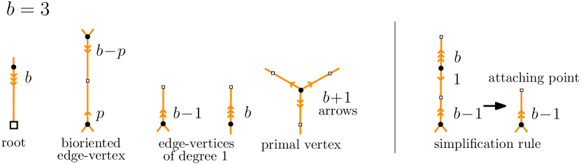
Figure 12: Environments of the various vertices in a $b$-arrow tree. For simplified $b$-arrow trees, non-root half-edges with $b$ arrows are removed as shown on the right.

Take a $b$-decorated tree corresponding to a $0$-slice, drawn on the derived map, and keep only the part of the tree drawn on the primal map, without the twigs. In other words, we keep only the primal half-edges which carry arrows and their incident vertices. This cuts the decorated tree into a number of connected components, which are themselves plane trees built out of both bioriented edges and oriented half-edges (corresponding to the primal half-edges incident to a bent edge-vertex). We shall call $b$-arrow trees these connected components. They are naturally planted by selecting as root the edge-vertex closest to the root of the $b$-decorated tree. A $b$-arrow tree is then characterized as follows (see Figure 12)

• it is made of primal vertices of degree at least two and edge-vertices of degree one or two, connected by primal half-edges carrying between $1$ and $b$ arrows;

• around each primal vertex there is a total number of arrows equal to $(b+1)$;

• around each edge-vertex of degree two (still called bioriented edge-vertex) there is a total number of arrows equal to $b$;

• next to each edge-vertex of degree one there are either $b-1$ or $b$ arrows, the root vertex having $b$.

Simplified $\boldsymbol{b}$-arrow trees.

For the purposes of enumeration, it is useful to slightly simplify the above characterization thanks to the following remark. Consider an edge-vertex of degree one with $b$ arrows which is not the root of the $b$-arrow tree. To fulfill the condition (ii), its adjacent primal vertex necessarily has degree two and has one arrow on the other side. Then it is in turn adjacent to a bioriented edge whose other half-edge carries $(b-1)$ arrows. We may thus at no cost remove this bivalent primal vertex and its two incident half-edges and keep only the remnant half-edge with $(b-1)$ arrows (see Figure 12-right and Figure 11-bottom right for an example). Doing so for each half-edge with $b$ arrows different from the root of the $b$-arrow tree, we end up with a slightly simpler notion of what we hereafter call simplified $b$-arrow trees, where point (iv) above is replaced by

• next to each edge-vertex of degree one different from the root, there are $b-1$ arrows. These edge-vertices will be called attaching points. Next to the root there are $b$ arrows.

Note that each attaching point of a simplified $b$-arrow tree may be equally connected to a special or a labeled dual vertex in the $b$-decorated tree, and that there is a unique way to make this connection: this requires $2$ additional half-edges and vertices to undo the simplification in the case where the dual vertex is labeled.

Blossoming vertices.

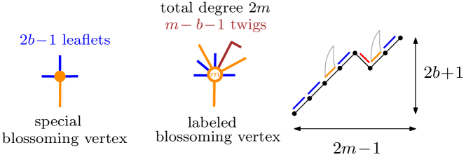
Figure 13: Representation of the order of decorations around blossoming vertices. Apart from their root, the special blossoming vertices are decorated with $2b-1$ leaflets, while labeled blossoming vertices with label $m$ are decorated with $m-b-1$ twigs and $m+b$ other decorations (interchangeably leaflets or attaching points). We represented on the left the proximity profile corresponding to the labeled blossoming vertex in the center, as defined in Figure 5. Each leaflet corresponds to an up step associated with an empty slice, each attaching point to an up step with an associated $0$-slice and each twig to a down step associated with a trivial slice. The example of labeled blossoming vertex shown here satisfies the tightness condition of Proposition 2.12.

If we now keep only the part of the original decorated tree drawn on the dual map and the twigs, all the dual vertices keep their degrees and we thus obtain a collection of blossoming vertices (see Figure 13) which are either special dual vertices of degree $2b$ or labeled dual vertices of degree $2m$ for some $m\geq b+1$. We will call the blossoming vertices special or labeled accordingly. Recall that a special blossoming vertex is decorated by $2b-1$ leaflets, and its incident half-edge incident to its parent bent edge-vertex will be called the root of this vertex. As for a labeled blossoming vertex of degree $2m$, its root is also the incident half-edge incident to its parent bent edge-vertex. The vertex is now decorated by $m-b-1$ twigs and a total of $m+b$ other half-edges, which are either leaflets or attaching points, which are the half-edges incident to its children bent edge-vertices in the decorated tree.

Note that we use the same denominations “root” and “attaching point” for the (primal) $b$-arrow trees and the (dual) blossoming vertices. In the decorated tree, the roots of blossoming vertices will be matched with the attaching points of the arrow trees, and vice versa.

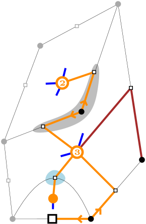
Figure 14: Example of a $1$-decorated tree. In gray and in light blue, the unique way to connect two labeled blossoming vertices (gray) or a labeled to a special blossoming vertex (light blue).

The case $\boldsymbol{b=1}$.

In the case $b=1$, the discussion is different, since the connection between faces can be achieved via dual/dual edge-vertices. We still have blossoming vertices of two types, special (with $2b-1=1$ leaflet) and labeled with $m-b-1=m-2$ twigs, which work similarly to the case $b>1$. What would correspond to $1$-arrow trees is a collection of either degree-two primal vertices, each connected to two regular bent edge-vertex (when linking two labeled vertices), or special dual/dual edge-vertices (when linking a special vertex to a labeled one). In all cases, for each attaching point of a labeled vertex, there is a unique corresponding blossoming vertex, and there is a unique way to make the connection (with two or four half-edges, depending on whether the other blossoming vertex is special or labeled). See Figure 14 for an example.

2.5 Characterization of tightness

So far, we did not impose that our slices be tight. A remarkable feature of the above decomposition of slices is that the tightness of the slice is entirely characterized by simple constraints on the decorations of the blossoming vertices in the associated decorated tree.

More precisely, recall that, in the context where there is no marked vertex, a slice is tight whenever it has no leaf. Assume on the contrary that the slice contains a leaf $L$, which is incident to a face $f$ of degree $2m$. We know that $m>b$, as otherwise the contour of the face would contain a cycle of size less than or equal to $2b-2$, which contradicts the $2b$-irreducibility. The face $f$ will therefore give rise to a blossoming vertex labeled $m$, which is built in a step (II). With $c_{s}$ the corner of $f$ incident to $L$ (see Figure 5 around vertex $L$, with $s=5$), we then know that:

• The proximity profile has $\ell_{s-1}=\ell_{s}+1=\ell_{s+1}$ ;

• The slice $\boldsymbol{\sigma}_{s}$ is the trivial slice ;

• The slice $\boldsymbol{\sigma}_{s+1}$ is the empty slice.

This latter property follows from the fact that the leftmost geodesic from $L$ starts with the only edge leaving $L$, which is also the base of the slice $\boldsymbol{\sigma}_{s+1}$. Conversely, if we find a trivial slice followed by an empty slice around $f$, then the identifications of the elementary slice boundaries shown on Figure 5 create a leaf. For the blossoming vertex associated with $f$, this translates into a decoration where a twig follows immediately (in clockwise order) a leaflet.

We thus have the following characterization:

Proposition 2.12 (Characterization of tightness).

A $2b$-irreducible slice (without marked vertices) is tight if and only if, at each blossoming vertex of the associated $b$-decorated tree, the sequence of decorations read in clockwise order around this vertex from its root does not contain the pattern of a twig followed immediately by a leaflet. A decorated tree with this property will be said to be tight.

3 Enumeration

Our goal is to obtain the expression (1) for the number $\mathcal{N}_{b}(m_{1},\ldots,m_{n})$ of planar bipartite tight $2b$-irreducible maps which can be constructed from a fixed number $n$ of labeled faces with prescribed even degrees $2m_{1},\ldots,2m_{n}$. From the bijection of Proposition 2.1 and the characterizations of Proposition 2.3, this can be done by enumerating, on the one hand, tight maps with two faces of prescribed degrees (and marked vertices) with a control on the length of their unique cycle and, on the other hand, sequences of tight $2b$-irreducible $0$-slices. Using the coding of $2b$-irreducible $0$-slices by $b$-decorated trees, this latter enumeration translates into the counting of sequences of $b$-decorated trees whose blossoming vertices are of a prescribed nature (i.e. special or labeled with a prescribed label) and satisfy the tightness characterization described in Proposition 2.12. Let us first proceed to the counting of $b$-decorated trees, where we start by enumerating sequences of (simplified) $b$-arrow trees (Section 3.1) and then combine them with blossoming vertices to obtain the desired sequences of $b$-decorated trees (Section 3.2).

3.1 Sequences of simplified arrow trees

Let us start with some notation:

Definition 3.1.

$\boldsymbol{\alpha_{k,n}^{(b)}:}$ Let $n$, $k$ and $b$ be non-negative integers with $b>1$. We denote by $\alpha_{k,n}^{(b)}$ the number of ordered $(k+1)$-uples of simplified $b$-arrow trees with a total of $n+1$ attaching points, one of them being distinguished in the first arrow tree.

When $b=1$, we did not use $b$-arrow trees for the decorated tree decomposition. Still, we define:

$$\alpha_{k,n}^{(1)}:=\delta_{k,n}$$ (5)

to account for the fact that there is a unique way to connect children blossoming vertices to their parent blossoming vertex (see Figure 14 and the related discussion at the end of Section 2.4). This connection is either via a dual/dual edge-vertex if the child is special, or via a pair of bent edge-vertices otherwise.

The goal of this section is to obtain an expression for $\alpha_{k,n}^{(b)}$ and to show that it is for $k\leq n$ a polynomial in $b$, of degree $2(n-k)$. Note that $\alpha_{k,n}^{(b)}$ vanishes for $k>n$ since a simplified $b$-arrow tree has at least one attaching point. Another related quantity of interest is the number $\mathcal{U}^{(b)}_{0,n}$ of simplified $b$-arrow trees with $n$ attaching points, for $n\geq 1$. We have the relation

$$\mathcal{U}^{(b)}_{0,n}=\frac{\alpha_{0,n-1}^{(b)}}{n},$$ (6)

as obtained upon forgetting the distinguished attaching point in the first and unique tree counted by $\alpha_{0,n-1}^{(b)}$.

Definition 3.2.

For $0\leq p\leq b-1$, we define a simplified $b$-arrow tree of excess $p$ as a tree which follows the rules (i), (ii) and (iii) of simplified $b$-arrow trees, but instead of (iv’) satisfies:

• next to each edge-vertex of degree one different from the root, there are $b-1$ arrows. These edge-vertices will be called attaching points. Next to the root there are $b-p$ arrows.

We denote by $\mathcal{U}^{(b)}_{p,n}$ the number of simplified $b$-arrow trees of excess $p$ with $n$ attaching points. Note that this notation is consistent with our definition of $\mathcal{U}^{(b)}_{0,n}$ just above, since simplified $b$-arrow trees are nothing but simplified $b$-arrow trees of excess $0$.

In the case $p=b-1$, when following the rules (i), (ii), (iii) and (iv”), the root edge (with one arrow) connects the root vertex to a primal vertex of degree at least three, so that there are at least two attaching points: as a consequence, $\mathcal{U}^{(b)}_{b-1,1}$ should a priori vanish. For convenience, we decide that the degenerate configuration of the tree consisting of a single edge-vertex, which serves both as root and as attaching point, is also considered as a simplified $b$-arrow tree of excess $p=b-1$. We therefore set accordingly

$$\mathcal{U}^{(b)}_{b-1,1}=1.$$ (7)

See Figure 15 for an illustration. The variable $p$ acts as a catalytic variable, as we are eventually interested in $\mathcal{U}^{(b)}_{0,n}$.

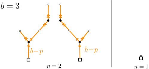
Figure 15: Examples of simplified $b$-arrow trees with excess $p=2$, when $b=3$. Left: the two possible cases with $n=2$ attaching points, leading to $\mathcal{U}^{(3)}_{2,2}=2$. Right: the degenerate configuration (which appears since $p=b-1$) with $n=1$ attaching point, leading to $\mathcal{U}^{(3)}_{2,1}=1$.

3.1.1 Elementary argument for the polynomiality in $b$

Starting from the root of a simplified $b$-arrow tree with excess $p$, we either are directly at an attaching point (if we are in the degenerate configuration, namely when $p=b-1$ and $n=1$), or, climbing the tree, the root is connected to an inner (primal) vertex. If this vertex is of degree $2$, then its unique child is counted by $\mathcal{U}^{(b)}_{p+1,n}$. We then climb the tree and cross all the vertices of degree $2$ until we reach an inner (primal) vertex with at least $2$ children, or an attaching point. More precisely, we reach an attaching point if and only if $n=1$, which yields

$$\mathcal{U}^{(b)}_{p,1}=1\qquad\hbox{for $0\leq p\leq b-1$.}$$ (8)

Assume $n>1$, we then reach an inner vertex with $q\geq 2$ children. We denote by $p_{1},\ldots,p_{q}\in\{1,\ldots,b-1\}$ the excesses of the corresponding children subtrees, and by $n_{1},\ldots,n_{q}\geq 1$ their respective numbers of attaching points. Clearly we have $n_{1}+\cdots+n_{q}=n$. We denote $s:=p_{1}+\cdots+p_{q}$. Then we have $p+1\leq s\leq b$: indeed, let us call $p_{0}$ the excess of the subtree just before we reach the vertex with $q$ children. We have $p\leq p_{0}\leq b-1$ since, by tree rules (ii) and (iv”), the excess increases by $1$ at each crossing of an inner (primal) vertex of degree $2$. Moreover, $(b-p_{0})+p_{1}+\cdots+p_{q}=b+1$ by the same rules, i.e. $s=p_{0}+1$.

As an example before we address the general case, let us first treat explicitly the case $n=2$. The only integer composition of $n=2$ yields $q=2$, $n_{1}=n_{2}=1$. We then have

$$\begin{split}\mathcal{U}^{(b)}_{p,2}&=\sum_{s=p+1}^{b}\sum_{\begin{subarray}{c}p_{1},p_{2}\geq 1\\ p_{1}+p_{2}=s\end{subarray}}\mathcal{U}^{(b)}_{p_{1},1}\mathcal{U}^{(b)}_{p_{2},1}=\sum_{s=p+1}^{b}\sum_{p_{1}=1}^{s-1}1=\sum_{s=p+1}^{b}(s-1)\\ &=\frac{b(b-1)}{2}-\frac{p(p-1)}{2}=\left[\frac{m(m-1)}{2}\right]_{p}^{b}.\end{split}$$ (9)

From this, we deduce $\alpha_{0,1}^{(b)}=2\mathcal{U}^{(b)}_{0,2}=b(b-1)$. More generally we can write $\alpha_{n-1,n}^{(b)}=(2+(n-1))\mathcal{U}^{(b)}_{0,2}\left(\mathcal{U}^{(b)}_{0,1}\right)^{n-1}$. Indeed, for $k=n-1$ we have exactly one arrow tree $\mathcal{T}_{2}$ with two attaching points, counted by $\mathcal{U}^{(b)}_{0,2}$, and $n-1$ other trees counted by $\mathcal{U}^{(b)}_{0,1}$. This yields $n$ different sequences according to the position of $\mathcal{T}_{2}$, each counted by $\mathcal{U}^{(b)}_{0,2}\left(\mathcal{U}^{(b)}_{0,1}\right)^{n-1}$. As we distinguish an attaching point in the first tree, this yields $2$ possibilities if $\mathcal{T}_{2}$ is in first position, and one possibility otherwise. Altogether, with $\mathcal{U}^{(b)}_{0,1}=1$ and $\mathcal{U}^{(b)}_{0,2}=\frac{b(b-1)}{2}$ we have

$$\alpha_{n-1,n}^{(b)}=\frac{n+1}{2}b(b-1).$$ (10)

The case $n=3$ is still doable by hand. We either have $q=2$ or $q=3$. When $q=3$, we have $n_{1}=n_{2}=n_{3}=1$, which yields after computations

$$\begin{split}\sum_{s=p+1}^{b}\sum_{\begin{subarray}{c}p_{1},p_{2},p_{3}\geq 1\\ p_{1}+p_{2}+p_{3}=s\end{subarray}}\mathcal{U}^{(b)}_{p_{1},1}\mathcal{U}^{(b)}_{p_{2},1}\mathcal{U}^{(b)}_{p_{3},1}&=\sum_{s=p+1}^{b}\sum_{p_{1}=1}^{s-1}\sum_{p_{2}=1}^{s-p_{1}-1}\mathcal{U}^{(b)}_{p_{1},1}\mathcal{U}^{(b)}_{p_{2},1}\mathcal{U}^{(b)}_{s-p_{1}-p_{2},1}\\ &=\left[\frac{m(m-1)(m-2)}{6}\right]_{p}^{b}.\end{split}$$ (11)

When $q=2$, we have the two symmetric cases $n_{1}=2,n_{2}=1$ and $n_{1}=1,n_{2}=2$. The first (and the second, by symmetry) is counted by

$$\begin{split}\sum_{s=p+1}^{b}\sum_{\begin{subarray}{c}p_{1},p_{2}\geq 1\\ p_{1}+p_{2}=s\end{subarray}}\mathcal{U}^{(b)}_{p_{1},2}\mathcal{U}^{(b)}_{p_{2},1}=&\sum_{s=p+1}^{b}\sum_{p_{1}=1}^{s-1}\mathcal{U}^{(b)}_{p_{1},2}\\ =&\sum_{s=p+1}^{b}\sum_{p_{1}=1}^{s-1}\left[\frac{m(m-1)}{2}\right]_{p_{1}}^{b}\\ =&\left[\frac{m(m-1)}{4}\left(b(b-1)-\frac{(m+1)(m-2)}{6}\right)\right]_{p}^{b}.\end{split}$$ (12)

Altogether, upon summing (11) and twice (12), we get

$$\begin{split}\mathcal{U}^{(b)}_{p,3}&=\left[\frac{m(m-1)(m-2)}{6}+2\frac{m(m-1)}{4}\left(b(b-1)-\frac{(m+1)(m-2)}{6}\right)\right]_{p}^{b}\\ &=\left[\frac{m(m-1)}{2}\left(b(b-1)-\frac{(m-1)(m-2)}{6}\right)\right]_{p}^{b}.\end{split}$$ (13)

We may then, from this formula and (9), derive the explicit expression:

$$\alpha_{n-2,n}^{(b)}=\frac{n+1}{6}\left(\frac{3n+4}{4}b+1\right)b(b-1)^{2}.$$ (14)

This follows from $\alpha_{n-2,n}^{(b)}=(3+(n-2))\mathcal{U}^{(b)}_{0,3}\left(\mathcal{U}^{(b)}_{0,1}\right)^{n-2}\!+(2(n-2)+\binom{n-2}{2})\!\left(\mathcal{U}^{(b)}_{0,2}\right)^{2}\!\left(\mathcal{U}^{(b)}_{0,1}\right)^{n-3}$ obtained similarly to the derivation of Equation (10). This is also a particular case of the general Equation (16) which we will see just below.

Let us now discuss the case of general $n$. We have the following:

Proposition 3.3.

For $b>1$, $n\geq 1$, $p\in\{0,\ldots b-1\}$, the quantity $\mathcal{U}^{(b)}_{p,n}$ is a polynomial in $b$ and $p$ of total degree $2(n-1)$, with a non-zero coefficient for $b^{2(n-1)}$.

Proof.

In the general case, we sum over all possible values of $q\geq 2$, over $n_{1},\ldots,n_{q}$ with sum $n$, over $s\geq p+1$, and over $p_{1},\ldots,p_{q}$ with sum $s$. The trick is that, for fixed $n$, we have a finite number of configurations of $q\in\left\{2,\ldots,n\right\}$ and $n_{1},\ldots,n_{q}\geq 1$ summing to $n$. We then have the recurrence formula, valid for $0\leq p\leq b-1$ and $n\geq 2$:

$$\mathcal{U}^{(b)}_{p,n}=\sum_{q=2}^{n}\sum_{\begin{subarray}{c}n_{1},\ldots,n_{q}\geq 1\\ n_{1}+\cdots+n_{q}=n\end{subarray}}\sum_{s=p+1}^{b}\sum_{\begin{subarray}{c}p_{1},\ldots,p_{q}\geq 1\\ p_{1}+\cdots+p_{q}=s\end{subarray}}\mathcal{U}^{(b)}_{p_{1},n_{1}}\cdots\mathcal{U}^{(b)}_{p_{q},n_{q}}$$ (15)

which allows us to prove Proposition 3.3 by recurrence. Indeed, the sum over $s$ and over the simplex of the $p_{1},\ldots,p_{q}$ is a discrete integration of dimension $q$ of the polynomial $\mathcal{U}^{(b)}_{p_{1},n_{1}}\cdots\mathcal{U}^{(b)}_{p_{q},n_{q}}$, which yields a polynomial of degree $2(n_{1}-1)+\cdots+2(n_{q}-1)+q=2n-q$ in $b$ and $p$. The dominant terms in the recurrence formula then come from the terms for $q=2$, with a total degree of $2(n-1)$, which, with initialization $\mathcal{U}^{(b)}_{p,1}=1$, concludes the recurrence for the total degree. Setting $p=0$ yields the degree $2(n-1)$ in $b$ alone. ∎

This leads to the following:

Corollary 3.4.

For $k\leq n$, $\alpha_{k,n}^{(b)}$ is a polynomial in $b$ of degree $2(n-k)$.

Proof.

We may retrieve, in the general case, the value of $\alpha_{k,n}^{(b)}$ by the formula:

$$\alpha_{k,n}^{(b)}=\sum_{\begin{subarray}{c}n_{1},\ldots,n_{k+1}\geq 1\\ n_{1}+\cdots+n_{k+1}=n+1\end{subarray}}n_{1}\mathcal{U}^{(b)}_{0,n_{1}}\cdots\mathcal{U}^{(b)}_{0,n_{k+1}}.$$ (16)

arising from Definition 3.1. In particular, since $\mathcal{U}^{(b)}_{0,n_{i}}$ is of degree $2(n_{i}-1)$ in $b$, $\alpha_{k,n}^{(b)}$ is a polynomial in $b$ of degree $2(n_{1}-1)+\cdots+2(n_{k+1}-1)=2(n+1)-2(k+1)=2(n-k)$. ∎

3.1.2 Direct formula via Lagrange inversion

Besides the above purely combinatorial approach, we may obtain a slightly more explicit direct (non-recursive) formula for $\alpha_{k,n}^{(b)}$ with an analytic approach based on a Lagrange inversion. More precisely, let us establish the expression (4) for $\alpha_{k,n}^{(b)}$, namely:

Proposition 3.5.

For $k,n$ non-negative integers and $b\geq 1$, we have

$$\alpha_{k,n}^{(b)}=[u^{n-k}]\frac{1}{\left(1+\sum\limits_{j=2}^{b}\frac{1}{b}\binom{b}{j}\binom{b}{j-1}(-u)^{j-1}\right)^{n+1}}.$$ (17)

Proof.

For $b=1$ this indeed yields $\alpha_{k,n}^{(1)}=\delta_{k,n}$ which is the desired value defined in Equation (5). Assume now $b>1$ and let $U_{0}(z)$ be the generating function of simplified $b$-arrow trees counted with a weight $z$ per attaching point. By Definition 3.1, we have

$$\alpha_{k,n}^{(b)}=[z^{n}]U_{0}^{\prime}(z)U_{0}(z)^{k}=\frac{n+1}{k+1}[z^{n+1}]U_{0}(z)^{k+1}.$$ (18)

More generally, for $0\leq p\leq b-1$, we introduce the generating function $U_{p}(z)$ of simplified $b$-arrow trees of excess $p$, still counted with a weight $z$ per attaching point. We may write

$$U_{p}(z)=\sum_{n\geq 1}\mathcal{U}^{(b)}_{p,n}z^{n},\qquad 0\leq p\leq b-1.$$ (19)

We may now obtain the formula:

$$U_{p}(z)=\sum_{q=1}^{p+1}\sum_{\begin{subarray}{c}p_{1},\ldots,p_{q}\geq 1\\ p_{1}+\cdots+p_{q}=p+1\end{subarray}}\prod_{j=1}^{q}U_{p_{j}}(z),\qquad 0\leq p\leq b-1,$$ (20)

with the convention $U_{b}(z):=z$. This values ensures that, when $p=b-1$, the $q=1$ term of the sum, which is equal to $U_{b}(z)$, gets the proper value $z$, consistent with (7). Equation (20) simply expresses the fact that, in a non-degenerate simplified $b$-arrow tree of excess $p$, the root vertex is connected to a primal vertex which has a number $q\geq 1$ of other neighbours which are edge-vertices. Removing this primal vertex and its incident primal half-edges, the tree is split into $q$ rooted subtrees, which are simplified $b$-arrow trees with respective excesses denoted $p_{1},\ldots,p_{q}$. From rules (ii), (iii) and (iv”), we get the constraint $p_{1}+\cdots+p_{q}=p+1$.

Note the similarity of this decomposition with the case (I) of the decomposition of $b$-irreducible $p$-slices: indeed, for $0\leq p\leq b-1$, $U_{p}(z)$ also counts $b$-irreducible $p$-slices with all inner faces of degree $2b$, each weighted by $z$.

Remark 3.6.

Note that Equation (20) can be obtained from Equation (15) by isolating the term $s=p+1$ in the latter and identifying the rest of the sum as $\mathcal{U}^{(b)}_{p+1,n}$, which yields:

$$\mathcal{U}^{(b)}_{p,n}=\mathcal{U}^{(b)}_{p+1,n}+\sum_{q=2}^{n}\sum_{\begin{subarray}{c}n_{1},\ldots,n_{q}\geq 1\\ n_{1}+\cdots+n_{q}=n\end{subarray}}\sum_{\begin{subarray}{c}p_{1},\ldots,p_{q}\geq 1\\ p_{1}+\cdots+p_{q}=p+1\end{subarray}}\mathcal{U}^{(b)}_{p_{1},n_{1}}\cdots\mathcal{U}^{(b)}_{p_{q},n_{q}},\qquad 0\leq p\leq b-1$$ (21)

with the convention that $\mathcal{U}^{(b)}_{b,n}:=\delta_{n,1}$ consistent with the convention $U_{b}(z)=z$. Then, translated in generating series, this yields

$$U_{p}(z)=U_{p+1}(z)+\sum_{q=2}^{p+1}\sum_{\begin{subarray}{c}p_{1},\ldots,p_{q}\geq 1\\ p_{1}+\cdots+p_{q}=p+1\end{subarray}}\prod_{j=1}^{q}U_{p_{j}}(z),\qquad 0\leq p\leq b-1$$ (22)

which is equivalent to Equation (20).

In its equivalent form (22), we see that the system (20) is triangular, as it may be rewritten

$$U_{p+1}(z)=U_{p}(z)-\sum_{q=2}^{p+1}\sum_{\begin{subarray}{c}p_{1},\ldots,p_{q}\geq 1\\ p_{1}+\cdots+p_{q}=p+1\end{subarray}}\prod_{j=1}^{q}U_{p_{j}}(z)$$ (23)

for $0\leq p\leq b-1$, where the sum in the right-hand side involves only $U_{1}(z),\ldots,U_{p}(z)$. It follows that $U_{p}(z)$ is a polynomial in $U_{0}(z)$ for all $p$. We may express it explicitly via the following trick, borrowed from [BG14, Section 5.4]: let us define $U_{p+1}(z)$ recursively for all $p\geq b$ via the relation (23). Note that, in this relation, we may take the sum over $q$ from $2$ to $\infty$, since the terms $q>p+1$ give no contribution. Then, in terms of the generating function $U(t,z):=\sum_{p\geq 1}U_{p}(z)t^{p}$, the relation yields

$$U(t,z)=t(U(t,z)+U_{0}(z))-\sum_{q=2}^{\infty}U(t,z)^{q}$$ (24)

which may be rewritten as

$$t=\frac{U(t,z)}{(1-U(t,z))(U(t,z)+U_{0}(z))}.$$ (25)

Using the Lagrange inversion formula, we obtain, for all $p\geq 1$,

$$U_{p}(z)=[t^{p}]U(t,z)=\frac{1}{p}[u^{p-1}]\left((1-u)(u+U_{0}(z))\right)^{p}=h_{p}(U_{0}(z))$$ (26)

where

$$h_{p}(u):=\sum_{j=1}^{p}\frac{(-1)^{j-1}}{p}\binom{p}{j}\binom{p}{j-1}u^{j}$$ (27)

is a polynomial in $u$, with zero constant term and with linear term $u$. Recalling that $U_{b}(z)=z$, we find that $U_{0}(z)$ is algebraic and determined implicitly by

$$z=h_{b}(U_{0}(z)).$$ (28)

Applying the Lagrange-Bürmann inversion formula to (18), we get

$$\alpha_{k,n}^{(b)}=\frac{n+1}{k+1}[z^{n+1}]U_{0}(z)^{k+1}=[u^{n-k}]\left(\frac{u}{h_{b}(u)}\right)^{n+1}$$ (29)

from which (17), hence (4), follows immediately. ∎

Pushing further the above computations, we may arrive at another expression for $\alpha_{k,n}^{(b)}$, which has the interest of being manifestly polynomial in $b$:

Proposition 3.7.

For $k,n$ non-negative integers, we have

$$\alpha_{k,n}^{(b)}=\sum_{s=0}^{\infty}(-1)^{n-k+s}\binom{n+s}{n}\sum_{\begin{subarray}{c}\ell_{1},\ldots,\ell_{s}\geq 1\\ \ell_{1}+\cdots+\ell_{s}=n-k\end{subarray}}r_{\ell_{1}}(b)\cdots r_{\ell_{s}}(b)$$ (30)

where

$$r_{\ell}(b):=\frac{1}{b}\binom{b}{\ell+1}\binom{b}{\ell}=\frac{1}{\ell!(\ell+1)!}\prod_{i=1}^{\ell}(b-i+1)(b-i)$$ (31)

is a polynomial of degree $2\ell$ in $b$. As a consequence, $\alpha_{k,n}^{(b)}$ is a polynomial of degree $2(n-k)$ in $b$ for $k\leq n$, and vanishes for $k>n$.

Let us remark that, in (30), the term $s=0$ contributes only for $k=n$, and the rightmost sum is then equal to $1$ as it involves a single term corresponding to the empty sequence: this yields $\alpha_{n,n}^{(b)}=1$ as wanted. For $k>n$, the rightmost sum vanishes for all $s$, since no sequence satisfies the wanted condition: this yields $\alpha_{k,n}^{(b)}=0$ as expected. Note finally that $r_{\ell}(0)=r_{\ell}(1)=0$ for all $\ell\geq 1$, and hence $\alpha_{k,n}^{(0)}=\alpha_{k,n}^{(1)}=\delta_{k,n}$ as wanted.

Proof of Proposition 3.7.

Observe that, in (27), we may replace the upper bound of the sum by $\infty$ since all terms $j>p$ have a zero contribution. Replacing $p$ by $b$, doing the change of variable $j=\ell+1$, and putting the first term apart, this allows to rewrite

$$h_{b}(u)=u+\sum_{\ell=1}^{\infty}(-1)^{\ell}r_{\ell}(b)u^{\ell+1}$$ (32)

with $r_{\ell}(b)$ as in the proposition. Plugging this expression in the right-hand side of (29), we get

$$\begin{split}\alpha_{k,n}^{(b)}&=[u^{n-k}]\frac{1}{\left(1+\sum_{\ell=1}^{\infty}(-1)^{\ell}r_{\ell}(b)u^{\ell}\right)^{n+1}}\\ &=[u^{n-k}]\sum_{s=0}^{\infty}(-1)^{s}\binom{n+s}{n}\left(\sum_{\ell=1}^{\infty}(-1)^{\ell}r_{\ell}(b)u^{\ell}\right)^{s}\end{split}$$ (33)

which gives the wanted formula (30). ∎

We list for bookkeeping purposes the following simple values for $k=n,n-1,n-2,n-3$:

• $\alpha_{n,n}^{(b)}=1$ for all $n$ ;

• $\alpha_{n-1,n}^{(b)}=\frac{n+1}{2}b(b-1)$ for $n\geq 1$, see Equation (10);

• $\alpha_{n-2,n}^{(b)}=\frac{n+1}{6}\left(\frac{3n+4}{4}b+1\right)b(b-1)^{2}$ for $n\geq 2$, see Equation (14);

• $\alpha_{n-3,n}^{(b)}=\frac{n+1}{12}\left(\frac{3n^{2}+9n+7}{12}b^{3}-\frac{3n^{2}-3n-11}{12}b^{2}-\frac{3n+2}{3}b-1\right)b(b-1)^{2}$ for $n\geq 3$.

3.2 Sequences of decorated trees

The purpose of this section is to establish the following:

Proposition 3.8.

For integers $n,b\geq 1$, $k\geq 0$ and $m_{1},\ldots,m_{n}\geq b$, the number of $(k+1)$-tuples of tight $b$-decorated trees having $n$ blossoming vertices of degrees $2m_{1},\ldots,2m_{n}$, where the first tree contains the blossoming vertex of degree $m_{1}$, is equal to

$$F^{(b)}_{k}(m_{1},\ldots,m_{n}):=(n-1)!\sum_{k_{1},\ldots,k_{n}\geq 0}q^{(b)}_{k_{1}}(m_{1})\cdots q^{(b)}_{k_{n}}(m_{n})\alpha^{(b)}_{k+k_{1}+\cdots+k_{n},n-1}$$ (34)

with $\alpha^{(b)}_{k,n}$ as in (4) and, recalling Equation (3),

$$q^{(b)}_{k}(m):=\binom{m+b}{k}\binom{m-b-1+k}{k}=\frac{1}{(k!)^{2}}\prod_{i=0}^{k-1}\left(m^{2}-(b-i)^{2}\right).$$ (35)

By the correspondence between decorated trees and slices, we immediately obtain the following:

Corollary 3.9.

For integers $n,b\geq 1$, $k\geq 0$ and integers $m_{1},\ldots,m_{n}\geq b$, the quantity $F^{(b)}_{k}(m_{1},\ldots,m_{n})$ in (34) is the number of $(k+1)$-tuples $(\mathbf{s}_{1},\ldots,\mathbf{s}_{k+1})$ of tight $2b$-irreducible $0$-slices such that there is a bijection between $\{1,\ldots,n\}$ and the union of the sets of the inner faces of $\mathbf{s}_{1},\ldots,\mathbf{s}_{k+1}$, such that each $j=1,\ldots,n$ is mapped to a face of degree $2m_{j}$, and $1$ is mapped to an inner face of $\mathbf{s}_{1}$. In particular, for $k=0$, the number of tight $2b$-irreducible $0$-slices with $n$ inner faces of degrees $2m_{1},\ldots,2m_{n}$ is equal to

$$F^{(b)}_{0}(m_{1},\ldots,m_{n})=(n-1)!\sum_{k_{1},\ldots,k_{n}\geq 0}q^{(b)}_{k_{1}}(m_{1})\cdots q^{(b)}_{k_{n}}(m_{n})\alpha^{(b)}_{k_{1}+\cdots+k_{n},n-1}.$$ (36)

Recall that $\alpha_{k,n}^{(b)}$ vanishes for $k>n$ hence the sums in (34) and (36) are finite sums.

The first step in the proof of Proposition 3.8 consists in observing that the quantity $q^{(b)}_{k}(m)$, which is a polynomial in $m^{2}$ and $b$, counts the number of possible decorations around a blossoming vertex of degree $2m$ with $k$ attaching points satisfying the tightness condition of Proposition 2.12. Indeed, for $m=b$ we have $q^{(b)}_{k}(b)=\delta_{k,0}$ as wanted for a special vertex which by definition has $0$ attaching point. For $m>b$, each decoration is coded by a word of length $2m-1$ over the alphabet $\{A,L,T\}$ (where these letters stand for attaching point, leaflet and twig respectively) with $k$ occurrences of $A$, $m+b-k$ occurrences of $L$ and $m-b-1$ occurrences of $T$, and no occurrence of the pattern $TL$. Such a word has the form

$$L^{i_{0}}T^{j_{0}}AL^{i_{1}}T^{j_{1}}A\cdots AL^{i_{k}}T^{j_{k}}$$ (37)

where $i_{0},i_{1},\ldots,i_{k}$ are non-negative integers summing to $m+b-k$ and $j_{0},j_{1},\ldots,j_{k}$ are non-negative integers summing to $m-b-1$. There are $\binom{m+b}{k}$ choices for the former and $\binom{m-b+k-1}{k}$ for the latter, leading to the expression (35).

The second step of the proof consists of the following:

Lemma 3.10.

Let $n,b,k,m_{1},\ldots,m_{n}$ be as in Proposition 3.8 and fix non-negative integers $k_{1},\dots,k_{n}$. Then, the number of tuples of decorated trees as in Proposition 3.8 where we add the requirement that, for each $i=1,\ldots,n$, the $i$-th blossoming vertex has exactly $k_{i}$ attaching points, is equal to $(n-1)!q^{(b)}_{k_{1}}(m_{1})\cdots q^{(b)}_{k_{n}}(m_{n})\alpha^{(b)}_{k+k_{1}+\cdots+k_{n},n-1}$.

Proof.

This results from general considerations on the enumeration of plane forests with labeled vertices, similar to those developed in [BGM24a, Appendix A].

Precisely, we first observe that for any $k_{0}\geq 0$, the quantity $(n-1)!\alpha^{(b)}_{k_{0},n-1}$ is the number of $(k_{0}+1)$-tuples of simplified $b$-arrow trees with a total of $n$ attaching points, that are numbered from $1$ to $n$, the one numbered $1$ being in the first arrow tree. Indeed, in $\alpha^{(b)}_{k_{0},n-1}$ there is a unique distinguished attaching point which is in the first tree, which we number $1$, and we have $(n-1)!$ ways to number the other attaching points. Now, we take $k_{0}=k+k_{1}+\cdots+k_{n}$, and for each $i=1,\ldots,n$ we choose a decoration for the $i$-th blossoming vertex in one of the $q^{(b)}_{k_{i}}(m_{i})$ ways, and attach the root of that blossoming vertex to the arrow tree attaching point numbered $i$. At this stage, we no longer have free attaching points incident to arrow trees, but we still have $k_{1}+\cdots+k_{n}=k_{0}-k$ free attaching points incident to blossoming vertices, while the number of trees is still $k_{0}+1$. There is then a canonical way to assemble these trees into a sequence of $(k_{0}+1)-(k_{0}-k)=k+1$ decorated trees with the first tree containing the first blossoming vertex. Indeed, we represent each of the $k_{0}+1$ tree by a sequence formed by a simple up step followed by a number of down steps equal to its number of free attaching points. This yields a sequence of steps with $k_{0}+1$ up steps and $k_{0}-k$ down steps. We write this sequence cyclically, and connect each down step with the closest available following up step with non-crossing arches; in the original trees, this corresponds to connecting the free attaching points to some of the roots. This yields a cyclic sequence of $k+1$ decorated trees, which we break into a linear sequence by demanding that the first blossoming vertex be in the first tree. This is precisely a tuple of decorated trees of the wanted type. ∎

From this lemma, Proposition 3.8 is deduced by summing over all possible $k_{1},\ldots,k_{n}$.

3.3 Two-face maps with marked vertices

Having enumerated $(k+1)$-tuples of tight $2b$-irreducible $0$-slices in the previous section, we are now left with the counting of maps $\mathbf{m}_{12}$ with two faces of prescribed degrees, and $(k+1)$ marked vertices. More precisely, it is the purpose of the present section to establish the following:

Proposition 3.11.

Let $k,c,m_{1},m_{2}$ be non-negative integers with $m_{1},m_{2}>c$. Then, the number $p^{(c)}_{k}(m_{1},m_{2})$ of tight planar maps with exactly two (labeled) faces of respective degrees $2m_{1}$ and $2m_{2}$, with $(k+1)$ among their vertices marked, one of them being distinguished, and with their unique cycle of length at least $2(c+1)$, is equal to

$$p^{(c)}_{k}(m_{1},m_{2})=\sum_{\begin{subarray}{c}k_{1},k_{2}\geq 0\\ k_{1}+k_{2}=k\end{subarray}}p^{(c)}_{k_{1}}(m_{1})q^{(c)}_{k_{2}}(m_{2})$$ (38)

with $q^{(c)}_{k_{2}}(m_{2})$ as in (3) or (35) with $b,k,m\to c,k_{2},m_{2}$, namely

$$q^{(c)}_{k_{2}}(m_{2})=\binom{m_{2}+c}{k_{2}}\binom{m_{2}-c-1+k_{2}}{k_{2}}=\frac{1}{(k_{2}!)^{2}}\prod_{i=0}^{k_{2}-1}\left(m_{2}^{2}-(c-i)^{2}\right)$$ (39)

and $p^{(c)}_{k_{1}}(m_{1})$ as in (2), namely

$$p^{(c)}_{k_{1}}(m_{1}):=\binom{m_{1}-c-1}{k_{1}}\binom{m_{1}+c+k_{1}}{k_{1}}=\frac{1}{(k_{1}!)^{2}}\prod_{i=1}^{k_{1}}\left(m_{1}^{2}-(c+i)^{2}\right).$$ (40)

Note that, borrowing from [BGM24a] the notation

$$p_{k,e}(m):=\binom{m+\frac{e}{2}-1}{k}\binom{m-\frac{e}{2}+k}{k}=\frac{1}{(k!)^{2}}\prod_{i=1}^{k}(m^{2}-(i-\frac{e}{2})^{2})$$ (41)

for $k\geq 0,e\in\mathbb{Z}$, we have $p^{(c)}_{k}(m)=p_{k,-2c}(m)$ and $q^{(c)}_{k}(m)=p_{k,2c+2}(m)$.

We emphasize that $p^{(c)}_{k}(m_{1},m_{2})$ counts two-face planar maps whose unique cycle has length at least $2(c+1)$. A first idea would be to count maps for which the unique cycle has a fixed length, and then perform a summation. While this may be done, see Remark 3.17 below, it is actually not the most direct route to the expression (38). Instead, we adapt the approach of [BGM24a, Sections 4.2 and 5.2] which relies on a bijection between two-face maps and pairs of sequences of trees with possibly different lengths.

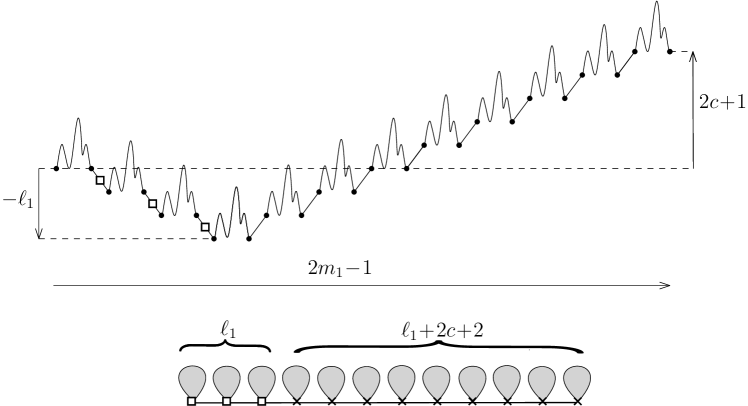
Figure 16: Top: a schematic picture of a word of the form (42), viewed equivalently as a lattice path with height difference $2c+1$ (here $c=2$). Calling $-\ell_{1}$ the minimum height (here $\ell_{1}=3$), we may decompose this path into $2\ell_{1}+2c+2$ blocks (Dyck paths) separated by $\ell_{1}$ down steps, which are markable (as indicated by squares) and $\ell_{1}+2c+1$ up steps. Bottom: alternatively, this codes for a sequence $\mathcal{S}_{1}$ of $2\ell_{1}+2c+2$ rooted plane trees (displayed as gray blobs connected by a spine of edges). The roots of the first $\ell_{1}$ trees can be marked or not (as indicated by squares). The roots of the last $\ell_{1}+2c+2$ trees are not marked (as indicated by crosses).

We first need to enumerate sequences of rooted plane trees, with some vertices marked, such that every leaf is marked. Such sequences are best encoded by concatenating Dyck paths with marked steps, where the marking of the leaves is enforced by forbidding a certain pattern. The sequences of such Dyck paths are themselves in one-to-one correspondence with appropriate words over a three-letter alphabet avoiding some pattern.

More precisely, take integers $c,k_{1}\geq 0$ and $m_{1}\geq c+1$, and consider words of length $2m_{1}-1$ over the alphabet $\{M,D,U\}$ (where these letters stand for marked-down, down and up respectively) with $k_{1}$ occurrences of $M$, $m_{1}-c-1-k_{1}$ occurrences of $D$ and $m_{1}+c$ occurrences of $U$, and with no occurrence of the pattern $UD$. Any such word has the form

$$D^{i_{0}}U^{j_{0}}MD^{i_{1}}U^{j_{1}}M\cdots MD^{i_{k_{1}}}U^{j_{k_{1}}}$$ (42)

where $i_{0},i_{1},\ldots,i_{k_{1}}$ are non-negative integers summing to $m_{1}-c-1-k_{1}$ and $j_{0},j_{1},\ldots,j_{k_{1}}$ are non-negative integers summing to $m_{1}+c$. There are $\binom{m_{1}-c-1}{k_{1}}$ choices for the former and $\binom{m_{1}+c+k_{1}}{k_{1}}$ for the latter, leading to the total number of words $p^{(c)}_{k_{1}}(m_{1})$ as in (40). Note that $p^{(c)}_{k_{1}}(m_{1})=0$ for $k_{1}\geq m_{1}-c$ as it should.

By interpreting the letter $U$ as coding for an elementary up step $(1,1)$, and the letter $D$ (respectively $M$) as coding for an elementary down step (respectively a marked elementary down step) $(1,-1)$, each word codes for a directed lattice path in $\mathbb{Z}^{2}$ starting at $(0,0)$, of total length (number of steps) equal to $(m_{1}+c)+(m_{1}-c-1-k_{1})+k_{1}=2m_{1}-1$, and height difference (final ordinate) equal to $(m_{1}+c)-(m_{1}-c-1-k_{1})-k_{1}=2c+1$. This path is equipped with a total of $k_{1}$ markings on the down steps. Calling $-\ell_{1}$ the minimal height of this path (see Figure 16), with $\ell_{1}\geq 0$ by construction, we can decompose the path into $2\ell_{1}+2c+2$ blocks separated by the $\ell_{1}$ down steps (that can be marked or not) which correspond to the first passage at height $h$ for $h=-1,\ldots,-\ell_{1}$ followed by the $\ell_{1}+2c+1$ up steps which correspond to the last passage at height $h$ for $h=-\ell_{1},\ldots,2c$. Each block is a Dyck path made of an equal number of up and down steps which, as is well-known, is the contour path of a rooted plane tree: recall that the contour path of a rooted plane tree with a total of $m$ non-root vertices is the path of length $2m$ obtained by going clockwise around the tree from its root and recording the distance to the root of the successive encountered corners. Each non-root vertex in the tree is in correspondence with a down step along the Dyck path (following the last passage at this vertex along the contour) and we may therefore transfer the markings of the down steps to their associated non-root vertices. The absence of the $UD$ pattern then guarantees that all the (non-root) leaves of the tree are marked. As for the root of the tree, we mark it if the block at hand is followed by a marked down step, which is possible only for the $\ell_{1}$ first blocks in the decomposition. Altogether, we arrive at the following:

Proposition 3.12.

For fixed integers $c,k_{1}\geq 0$ and $m_{1}\geq c+1$, the number of sequences $\mathcal{S}_{1}$ made of $2\ell_{1}+2c+2$ rooted plane trees with a total of $m_{1}-(c+1)-\ell_{1}$ internal edges, for some (unfixed) value $\ell_{1}$ with $0\leq\ell_{1}\leq m_{1}-(c+1)$ , with a total of $k_{1}$ marked vertices and such that all the (non-root) leaves of the trees are marked and the roots of the last $\ell_{1}+2c+2$ plane trees are not marked is given by $p^{(c)}_{k_{1}}(m_{1})$ as in (40).

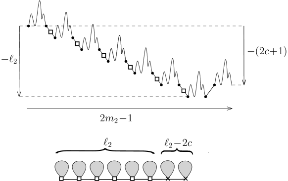
Figure 17: Top: a lattice path with height difference $-(2c+1)$ having minimal height $-\ell_{2}$ (with $\ell_{2}\geq 2c+1$, here $c=2$ and $\ell_{2}=6$). We may decompose this path as in Figure 16, creating now $2\ell_{2}-2c$ blocks (Dyck paths). Bottom: alternatively, this codes for a sequence $\mathcal{S}_{2}$ of $2\ell_{2}-2c$ rooted plane trees (displayed as gray blobs connected by a spine of edges), where the roots of the first $\ell_{2}$ trees are markable, while the roots of the last $\ell_{2}-2c$ are not.

Take now integers $c,k_{2}\geq 0$ and $m_{2}\geq c+1$ and consider words of length $2m_{2}-1$ over the alphabet $\{M,D,U\}$ with $k_{2}$ occurrences of $M$, $m_{2}+c-k_{2}$ occurrences of $D$ and $m_{2}-c-1$ occurrences of $U$, again with no occurrence of the pattern $UD$. As seen from the direct correspondence $M\to A$, $D\to L$, $U\to T$, $c\to b$, $k_{2}\to k$ and $m_{2}\to m$ with the calculation presented in the proof of Proposition 3.8, the total number of words with the above requirement is now $q^{(c)}_{k_{2}}(m_{2})$ as in (39). Note that $q^{(c)}_{k_{2}}(m_{2})=0$ for $k_{2}\geq m_{2}+c+1$ as it should. Each word now codes for a lattice path of total length $2m_{2}-1$ and height difference $-(2c+1)$, see Figure 17. Calling $-\ell_{2}$ the minimal height of this path, with $\ell_{2}\geq 2c+1$ by construction, we can decompose the path into $2\ell_{2}-2c$ blocks which are Dyck paths coding for rooted plane trees. As before, we transfer the markings of the down steps within a Dyck path to their associated non-root vertices in the associated plane tree. The absence of the $UD$ pattern then guarantees that all the (non-root) leaves of the trees are marked. As for the root of the trees, we mark them if the block at hand is followed by a marked down step, which is possible only for the $\ell_{2}$ first blocks in the decomposition. Altogether, we arrive at the following:

Proposition 3.13.

For fixed integers $c,k_{2}\geq 0$ and $m_{2}\geq c+1$, the number of sequences $\mathcal{S}_{2}$ made of $2\ell_{2}-2c$ rooted plane trees with a total of $m_{2}+c-\ell_{2}$ internal edges, for some (unfixed) value $\ell_{2}$ with $2c+1\leq\ell_{2}\leq m_{2}+c$ , with a total of $k_{2}$ marked vertices and such that all the (non-root) leaves of the trees are marked and the roots of the last $\ell_{2}-2c$ plane trees are not marked is given by $q^{(c)}_{k_{2}}(m_{2})$ as in (39).

We are now ready for the proof of Proposition 3.11.

Proof of Proposition 3.11.

As in [BGM24a], we use the fact that a planar map with two faces can be built out of two sequences of plane trees by sticking them together. Consider more precisely a sequence $\mathcal{S}_{1}$ of plane trees as defined in Proposition 3.12 and call $2\ell_{1}+2c+2$ the length of this sequence, with $\ell_{1}\geq 0$. Consider also a sequence $\mathcal{S}_{2}$ of plane trees as defined in Proposition 3.13 and call $2\ell_{2}-2c$ the length of this sequence, with $\ell_{2}\geq 2c+1$. As in Figure 16 (resp. Figure 17), we transform the sequence $\mathcal{S}_{1}$ (resp. $\mathcal{S}_{2}$) into a single connected object by attaching the trees with a spine made of $2\ell_{1}+2c+1$ (resp. $2\ell_{2}-2c-1$) elementary edges.

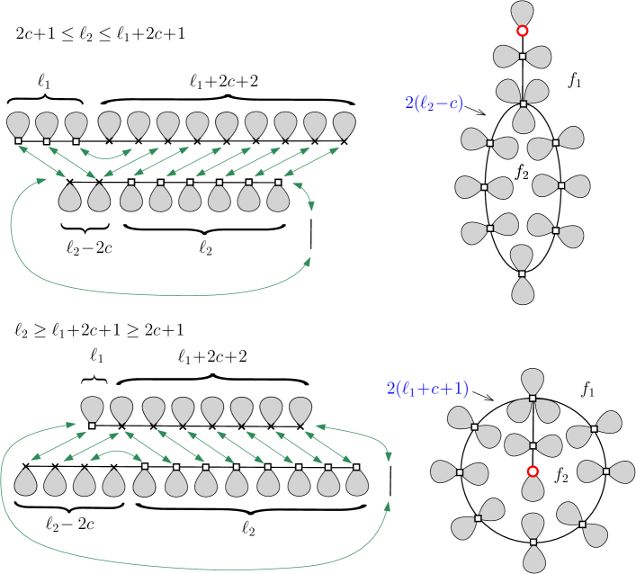
Figure 18: The gluing of two sequences of rooted trees into a two-face map (see text) according to whether $\ell_{2}$ lies between $2c+1$ and $\ell_{1}+2c+1$ (top) or is larger than or equal to $\ell_{1}+2c+1$ (bottom). The green arrows indicate which vertices to identify in the gluing process. In both case, the length of the separating loop (indicated in blue) is larger than or equal to $2(c+1)$. Squares indicate markable vertices and crosses non-markable ones. The red circle indicates the mandatory marking of the distinguished vertex.

Assume first that $\ell_{2}\leq\ell_{1}+2c+1$ so that the spine of $\mathcal{S}_{1}$ is longer than (or of the same length as) that of $\mathcal{S}_{2}$. We then shorten the spine of $\mathcal{S}_{1}$ by pulling up the $(\ell_{1}+1)$-th tree and by zipping the spine so as to attach the root of the $(\ell_{1}+1-j)$-th tree to that of the $(\ell_{1}+1+j)$-th one for $j=1,\ldots,\ell_{1}+2c+1-\ell_{2}$. This creates a shorter spine of length $2\ell_{2}-2c-1$ with we may now glue “face to face” with the spine of $\mathcal{S}_{2}$ and close it into a cycle of length $2(\ell_{2}-c)$ by adding an extra closing edge as shown in Figure 18-top. The final result is a map with two faces $f_{1}$ and $f_{2}$ of respective degrees $2\times(m_{1}-(c+1)-\ell_{1})+2\ell_{1}+2c+2=2m_{1}$ and $2\times(m_{2}+c-\ell_{2})+2\ell_{2}-2c=2m_{2}$ with separating cycle of length $\mathcal{L}=2(\ell_{2}-c)$ with an additional distinguished marked vertex incident to $f_{1}$ corresponding to the endpoint of the zip, leading to a total of $k_{1}+k_{2}+1$ marked vertices (and all the leaves marked). Note that the gluing procedure is such that a markable vertex is always glued to an unmarked one and the tip of the zip is initially not marked. These two conditions are crucial to ensure that all vertices are markable in the two-face map and that the construction is reversible without ambiguity as to which side to assign vertex markings after unzipping. Note also that the additional marking is needed to know where and how far to unzip. Finally, since $\ell_{2}\geq 2c+1$, we deduce that $\mathcal{L}\geq 2(c+1)$.

Assume now that $\ell_{2}\geq\ell_{1}+2c+1$ so that the spine of $\mathcal{S}_{1}$ is shorter than (or of the same length as) that of $\mathcal{S}_{2}$. We now shorten this latter spine by pulling down the $(\ell_{2}+1)$-th tree (counted from the right on Figure 18-bottom) and by zipping the spine so as to attach the root of the $(\ell_{2}+1-j)$-th tree to that of the $(\ell_{2}+1+j)$-th one for $j=1,\ldots,\ell_{2}-(\ell_{1}+2c+1)$. The two spines then have the same length $2\ell_{1}+2c+1$ and we may again glue them and close the resulting segment into a cycle of length $2(\ell_{1}+c+1)$ by adding an extra closing edge. The final result is again a map with two faces $f_{1}$ and $f_{2}$ of respective degrees $2m_{1}$ and $2m_{2}$ with now a separating cycle of length $\mathcal{L}=2(\ell_{1}+c+1)$ with an additional distinguished marked vertex incident to the face $f_{2}$ (leading to a total of $k_{1}+k_{2}+1$ marked vertices). Again the gluing procedure is such that a markable vertex is always glued to an unmarked one and the tip of the zip is initially not marked, as required to ensure that all vertices are markable in the two-face map and that the construction is reversible without ambiguity. Finally, since $\ell_{1}\geq 0$, we deduce that, again, $\mathcal{L}\geq 2(c+1)$.

Note that if $\ell_{2}=\ell_{1}+2c+1$, both constructions are fully identical: this corresponds to the case where no zipping is necessary and the additional marked vertex is on the separating loop itself.

This ends the proof of Proposition 3.11 by summing over $k_{1}$ and $k_{2}$ with $k_{1}+k_{2}=k$. ∎

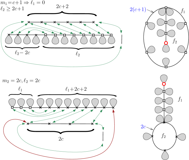
Figure 19: Top: limit case of the gluing of Figure 18-bottom. Taking $m_{1}=c+1$ implies that $\ell_{1}=0$ and yields a two-face map where the face $f_{1}$ is simple, and its incident vertices are all markable. This is counted by $q^{(c)}_{k}(m_{2})$ if $f_{2}$ has degree $2m_{2}$ (and there is a total of $k+1$ markings, one being distinguished). Bottom: degenerate case $m_{2}=c$. The gluing now yields a two-face map where the face $f_{2}$ is simple, and its incident vertices are non-markable. This degenerate case is not a particular case of the gluing of Figure 18-top, since here the separating loop has length $2c$. The vertices of the empty spine are non-markable, and the zipping matches the rightmost tree of $\mathcal{S}_{1}$ with the leftmost vertex of $\mathcal{S}_{2}$ (see the brown arrow). This is counted by $p^{(c)}_{k}(m_{1})$ if $f_{1}$ has degree $2m_{1}$ (and there is a total of $k+1$ markings, one being distinguished).

Remarks.

We end this section with some remarks regarding the quantity $p^{(c)}_{k}(m_{1},m_{2})$.

Remark 3.14.

In the case $m_{1}=c+1$, we have $p^{(c)}_{k_{1}}(m_{1})=\delta_{k_{1},0}$, so that (38) reduces, via $k_{2}=k$, to

$$p^{(c)}_{k}(c+1,m_{2})=q^{(c)}_{k}(m_{2}).$$ (43)

This gives a direct interpretation of $q^{(c)}_{k}(m_{2})$ which can be recovered as follows: we already know that $q^{(c)}_{k}(m_{2})$ counts the sequences $\mathcal{S}_{2}$ of Proposition 3.13. The requirement $m_{1}=c+1$ forces that $\ell_{1}=0$ (recall that $0\leq\ell_{1}\leq m_{1}-(c+1)$), and that $\mathcal{S}_{1}$ is the empty spine of length $2c+1$, composed of $2c+2$ non-markable vertices, with all the trees reduced to their root vertex. When zipping $\mathcal{S}_{2}$ to match it (see Figure 19, top), we end up with a map with a face of degree $2m_{2}$ and a simple face of degree $2c+2$, where the cycle is also the contour of this simple face, and all the vertices of this cycle are markable. As before, this map has $k+1$ markings, one of them distinguished, and all its leaves are marked.

Remark 3.15.

Proposition 3.11 assumes that $m_{1},m_{2}>c$. In the case $m_{2}=c$, we have $q^{(c)}_{k_{2}}(m_{2})=\delta_{k_{2},0}$, so that (38) reads, via $k_{1}=k$,

$$p^{(c)}_{k}(m_{1},c)=p^{(c)}_{k}(m_{1}).$$ (44)

This leads to a new interpretation of $p^{(c)}_{k}(m_{1},m_{2})$ when $m_{2}=c$, from the following direct interpretation of $p^{(c)}_{k}(m_{1})$: we already know that $p^{(c)}_{k}(m_{1})$ counts the sequences $\mathcal{S}_{1}$ of Proposition 3.12. If we now replace $\mathcal{S}_{2}$ by the empty spine of length $2c-1$ (composed of $2c$ non-markable vertices with all the trees reduced to their root vertex), and zip $\mathcal{S}_{1}$ to match it (see Figure 19, bottom), we end up with a map with a face of degree $2m_{1}$ and a simple face of degree $2c$, where the cycle is also the contour of this simple face, and all the vertices of this cycle are now non-markable. As always, this map has $k+1$ markings, one of them distinguished, and all its leaves are marked. This interpretation of $p^{(c)}_{k}(m_{1})$, or equivalently of $p^{(c)}_{k}(m_{1},m_{2})$ when $m_{2}=c$, will be useful in the next remarks, as well as for our main theorem 1.1.

Remark 3.16.

We have the relation

$$q_{k}^{(c)}(m)=\sum_{i=0}^{k}\binom{2c+1}{i}p_{k-i}^{(c)}(m)$$ (45)

which can be understood as follows: according to Remark 3.15, $p_{k-i}^{(c)}(m)$ counts two-face maps with a total of $k+1-i$ marked vertices, one distinguished, with a simple face $f_{0}$ of degree $2c$ having no incident marked vertex, the other face being of degree $2m$. In particular, the distinguished marked vertex is not incident to $f_{0}$ and the branch leading from $f_{0}$ to this vertex has no-zero length. We may unzip the first edge of this branch so as to obtain a larger simple face $f^{\prime}_{0}$ of degree $2c+2$ and a shorter (by one edge) branch. None of the vertices incident to $f^{\prime}_{0}$ are marked, except possibly the incident vertex at the beginning of the new branch leading to the distinguished vertex (note that this branch may be reduced to the distinguished vertex itself). If we now mark $i$ among the $2c+1$ other vertices incident to $f^{\prime}_{0}$, which can be done in $\binom{2c+1}{i}$ ways, we end up with a two-face map with a simple face of degree $2c+2$, the other face being still of degree $2m$, with a total of $k+1$ marked vertices, one of them distinguished and exactly $i$ marked vertices along its unique cycle deprived of its vertex incident to the branch leading to the distinguished vertex. Summing over $i$, this enumerates precisely maps counted by $q_{k}^{(c)}(m)$ according to Remark 3.14.

From (45), we get the alternative expression

$$p_{k}^{(c)}(m_{1},m_{2})=\sum_{\begin{subarray}{c}k_{1},k_{2},i\geq 0\\ k_{1}+k_{2}+i=k\end{subarray}}\binom{2c+1}{i}p_{k_{1}}^{(c)}(m_{1})p_{k_{2}}^{(c)}(m_{2}).$$ (46)

which displays that $p_{k}^{(c)}(m_{1},m_{2})$ is indeed symmetric in its two arguments as it should.

Remark 3.17.

For bookkeeping purposes, let us mention another approach to computing $p^{(c)}_{k}(m_{1},m_{2})$. Let us denote by $o^{(d)}_{k}(m_{1},m_{2})$ the number of planar tight maps with exactly two (labeled) faces of respective degrees $2m_{1}$ and $2m_{2}$, with $(k+1)$ among their vertices marked, one of them being distinguished, and with their unique cycle of length exactly $2d$. As $p^{(c)}_{k}(m_{1},m_{2})$ corresponds to two-face maps whose cycle has length at least $2(c+1)$, we have, for $m_{1},m_{2}\geq c+1$,

$$p^{(c)}_{k}(m_{1},m_{2})=\sum_{d\geq c+1}o^{(d)}_{k}(m_{1},m_{2}).$$ (47)

Then, in terms of the same univariate polynomials $p_{k}^{(c)}(m)$ and $q_{k}^{(c)}(m)$ as above, we have the expression

$$o^{(d)}_{k}(m_{1},m_{2})=\sum_{\begin{subarray}{c}\kappa_{1},\kappa_{2}\geq 1\\ \kappa_{1}+\kappa_{2}=k+1\end{subarray}}\frac{(2d)(\kappa_{1}+\kappa_{2})}{\kappa_{1}\kappa_{2}}p^{(d)}_{\kappa_{1}-1}(m_{1})q^{(d-1)}_{\kappa_{2}-1}(m_{2})\\ +p^{(d)}_{k}(m_{1})\delta_{m_{2},d}+\delta_{m_{1},d}q^{(d-1)}_{k}(m_{2})$$ (48)

which may be combinatorially interpreted as follows. Consider a map contributing to $o^{(d)}_{k}(m_{1},m_{2})$: cutting along its unique cycle and filling the holes with new simple faces $\tilde{f}_{1}$ and $\tilde{f}_{2}$ of degree $2d$, we get, upon transferring the markings to face $f_{2}$: on one hand a two-face map $\mathcal{Q}$ with a simple face $\tilde{f}_{1}$ and the initial face $f_{2}$, and on the other hand a two-face map $\mathcal{P}$ with a simple face $\tilde{f}_{2}$ and the initial face $f_{1}$ without markings incident to the face $\tilde{f}_{2}$. Calling $\kappa_{1}$ and $\kappa_{2}$ the total number of markings in $\mathcal{Q}$ and $\mathcal{P}$ respectively, those maps are the two types of maps considered respectively in Remarks 3.14 (with $c=d-1,k=\kappa_{1}-1$) and 3.15 (with $c=d,k=\kappa_{2}-1$), except we miss the distinguished marked vertex in one of those faces. After correcting this problem, since there are $2d$ ways to reassemble the maps $\mathcal{P}$ and $\mathcal{Q}$, this gives a number of possibilities equal to $(2d)p^{(d)}_{\kappa_{1}-1}(m_{1})q^{(d-1)}_{\kappa_{2}-1}(m_{2})$. Doing so, we obtain a two-face map with a pair of distinguished vertices (one incident to $f_{2}$, and one incident to $f_{1}$ but not $f_{2}$). Starting from a two-face map without distinguished vertices, there are $\kappa_{1}\kappa_{2}$ ways to choose such pairs, and $\kappa_{1}+\kappa_{2}$ ways to choose one distinguished vertex in the whole map, so, to correct the above problem, we multiply the preceding expression by $\frac{\kappa_{1}+\kappa_{2}}{\kappa_{1}\kappa_{2}}$. Summing over $\kappa_{1}+\kappa_{2}=k+1$ we get the first term in Equation (48).

The extra terms on the second line correspond to the pathological situation where there is no marked vertex incident to one of the faces, forcing the corresponding sequence of trees to contain only trees reduced to their root vertex. We have checked by computer algebra that the expressions (38) and (47) match for the first values of $k$, and one might look for a general algebraic proof, besides the combinatorial proof that we sketched here.

3.4 The final result: enumeration of tight irreducible maps

We are now ready to prove Theorem 1.1 via the following:

Proposition 3.18.

For integers $n\geq 3$, $b,c\geq 1$, $m_{1},m_{2}\geq c+1$, and $m_{3},\ldots,m_{n}\geq b$, the number of planar bipartite tight maps with $n$ labeled faces of respective degrees $2m_{1},\ldots,2m_{n}$ which are essentially $2b$-irreducible (as defined in Proposition 2.3) and have separating girth at least $2(c+1)$ is equal to

$$(n-3)!\sum_{k,k_{3},\ldots,k_{n}\geq 0}p^{(c)}_{k}(m_{1},m_{2})q^{(b)}_{k_{3}}(m_{3})\cdots q^{(b)}_{k_{n}}(m_{n})\alpha^{(b)}_{k+k_{3}+\cdots+k_{n},n-3}.$$ (49)

Note again that $\alpha_{k,n}^{(b)}=0$ for $k>n$ hence the sum in (49) is finite.

Proof.

By Proposition 2.3, we need to enumerate tuples of the form $(\mathbf{m}_{12},\mathbf{s}_{1},\ldots,\allowbreak\mathbf{s}_{k+1})$ as in Proposition 2.1, where furthermore the unique cycle of $\mathbf{m}_{12}$ has length at least $2(c+1)$, and where $\mathbf{s}_{1},\ldots,\mathbf{s}_{k+1}$ are $2b$-irreducible. Proposition 3.11 enumerates the former and Corollary 3.9 the latter, upon changing $n$ into $n-2$ and shifting the face labels by $2$. By summing over $k$, the wanted number reads

$$\sum_{k\geq 0}p^{(c)}_{k}(m_{1},m_{2})F^{(b)}_{k}(m_{3},\ldots,m_{n})$$ (50)

which yields (49) by (34). ∎

We may now proceed to the:

Proof of Theorem 1.1.

The expression (1) for $\mathcal{N}_{n}^{(b)}(2m_{1},\ldots,2m_{n})$ is obtained:

• in the case $m_{2}>b$ as a direct corollary of Proposition 3.18, using the fifth item in Proposition 2.3 and the expression (38) for $p^{(c)}_{k}(m_{1},m_{2})$ with $c=b$,

• in the case $m_{2}=b$ as a direct consequence of the sixth item in Proposition 2.3 and of the interpretation of Remark 3.15 for $p^{(c)}_{k}(m_{1},m_{2})$ when $m_{2}=c=b$.

Let us now verify the polynomiality properties of $\mathcal{N}_{n}^{(b)}(2m_{1},\ldots,2m_{n})$. From their expressions (39) and (40) with $c\to b$, $p^{(b)}_{k_{i}}(m_{i})$ and $q^{(b)}_{k_{i}}(m_{i})$ are polynomials of total degree $2k_{i}$ in $b$ and $m_{i}$ (and even in $m_{i}$). Recall that $\alpha_{k,n-3}^{(b)}$ vanishes for $k>n-3$ and that for $k\leq n-3$ it is by Corollary 3.4 or Proposition 3.7 a polynomial of degree $2(n-3-k)$ in $b$. Therefore, each non-zero term in the sum in (1) is of degree $2(n-3-\sum_{i}k_{i})+2\sum_{i}k_{i}=2n-6$ in $b$ and the $m_{i}$’s. Its top degree term in the $m_{i}$’s is $\prod_{i}\frac{m_{i}^{2k_{i}}}{(k_{i}!)^{2}}$ which, for $\sum_{i}k_{i}=n-3$, is not present in any other non-zero term. Thus, the total degree of $\mathcal{N}_{n}^{(b)}(2m_{1},\ldots,2m_{n})$ is exactly $2n-6$. The expression (1) is clearly symmetric in $m_{2},\ldots,m_{n}$, and also symmetric upon exchanging $m_{1}$ and $m_{2}$, as proved in Remark 3.16, hence it is symmetric in all its arguments. ∎

The formula (1) given in this paper can be identified as [Bud22, Equation (66)], as discussed in Appendix B.

Particular cases.

Using $q^{(b)}_{k}(b)=p^{(b)}_{k}(b+1)=\delta_{k,0}$, we have the following specializations:

Proposition 3.19.

For $n\geq 3$ and $m_{1},m_{2}\geq b$ not both equal to $b$, we have

$$\mathcal{N}_{n}^{(b)}(2m_{1},2m_{2},\underbrace{2b,\ldots,2b}_{n-2\text{ times}})=(n-3)!\sum_{k=0}^{n-3}p_{k}^{(b)}(m_{1},m_{2})\alpha_{k,n-3}^{(b)}.$$ (51)

Proposition 3.20.

For $n\geq 3$ and $m>b$, we have

$$\mathcal{N}_{n}^{(b)}(2m,\underbrace{2b,\ldots,2b}_{n-1\text{ times}})=(n-3)!\sum_{k=0}^{n-3}p_{k}^{(b)}(m)\alpha_{k,n-3}^{(b)},$$ (52)

$$\mathcal{N}_{n}^{(b)}(2m,2b+2,\underbrace{2b,\ldots,2b}_{n-2\text{ times}})=(n-3)!\sum_{k=0}^{n-3}q_{k}^{(b)}(m)\alpha_{k,n-3}^{(b)}.$$ (53)

Proposition 3.21.

For $n\geq 3$, we have

$$\mathcal{N}_{n}^{(b)}(2b+2,\underbrace{2b,\ldots,2b}_{n-1\text{ times}})=(n-3)!\alpha_{0,n-3}^{(b)}.$$ (54)

For $b=2$ and $n\geq 3$, this yields

$$\mathcal{N}_{n}^{(2)}(6,\underbrace{4,\ldots,4}_{n-1\text{ times}})=\frac{(2(n-3))!}{(n-3)!}$$ (55)

for the number of $4$-irreducible dissections of the hexagon by $(n-1)$ labeled quadrangles, in agreement with [MS68] and [FSP08]. Indeed, the tightness (and even the $2$-connectedness) of the map follows automatically from the irreducibility constraints.

Finally, recalling Remark 2.4 (with $n\to n+2$) and Corollary 3.9, we get:

Proposition 3.22.

For $n\geq 1$ and $m_{1},\ldots,m_{n}\geq b$, we have

$$\mathcal{N}_{n+2}^{(b)}(2b+2,2b,2m_{1},\ldots,2m_{n})=F_{0}^{(b)}(m_{1},\ldots,m_{n})\\ =(n-1)!\sum_{k_{1},\ldots,k_{n}\geq 0}q^{(b)}_{k_{1}}(m_{1})\cdots q^{(b)}_{k_{n}}(m_{n})\alpha^{(b)}_{k_{1}+\cdots+k_{n},n-1}.$$ (56)

4 Conclusion

In this paper, we gave a fully combinatorial proof of Theorem 1.1 counting the number of planar bipartite tight $2b$-irreducible maps with labelled faces of prescribed degrees. As opposed to Budd’s approach in [Bud22] based on a substitution of formal power series, we had recourse here to a decomposition of desired maps into (tight $2b$-irreducible) slices for which we presented a bijective enumeration based on $b$-decorated trees drawn on their derived map.

Even though we have not worked out the details, we believe that the assumption of bipartiteness is not essential, and our formula can be extended to the enumeration of planar tight $d$-irreducible maps with labelled faces of arbitrary odd or even degrees. The case $d=0$ was treated in detail in [BGM24a, Theorem 2.12] and involves quasi-polynomials instead of ordinary polynomials.

The decorated tree formulation of Section 2.3 involves placing arrows on the primal half-edges of the map, which form arrow trees. Such construction is strongly reminiscent of the approach of Bernardi and Fusy, which consists in choosing an appropriate biorientation of the map. We noted in Remark 2.11 that, in the absence of special vertices (which corresponds to maps with no face of degree $2b$), our $b$-decorated trees correspond precisely to the $(b+1)$-dibranching mobiles of [BF12a, Definition 8]. Reintroducing the faces of degree $2b$ in their formulation seems to add an extra challenge, and we wonder whether the ideas of [BFL23], which involve working with orientations of the derived map, could solve this issue.

Finally, we cannot help but notice that the general structure of the right-hand side of Equation (1) is very reminiscent of [BGM24, Equation (32)] for planar bipartite maps with a number of labelled tight boundaries of prescribed degrees (and arbitrary even-valent internal faces).

Appendix A Going back from a decorated tree to a $\boldsymbol{0}$-slice

We discuss here how to get back from a $b$-decorated tree for some $b\geq 1$ to the associated tight $2b$-irreducible $0$-slice. In practice we rather construct the dual map of the $0$-slice by a classical procedure of closure consisting in matching the leaflets of the decorated tree to properly placed buds via a system of non-crossing arches.

The first step of the construction consists in adding buds to the decorated tree as follows (see Figure 20). We first complete the decorated tree by adding a dual half-edge from its univalent root edge-vertex $v_{0}$ to a dual vertex $\Delta_{0}$ in the outer face. Then, all edge-vertices have degree two in the (completed) decorated tree while they had degree four in the derived map. The added buds then correspond to the missing incident dual half-edges. More precisely, an edge-vertex $v$ of the decorated tree may be a bioriented edge-vertex and we then attach to $v$ two buds, one in each corner around $v$ in the decorated tree (to account for the fact that $v$ should be incident to two dual half-edges not covered by the tree in the derived map). The vertex $v$ may be a bent edge-vertex: we then attach one bud to $v$ (to account for the fact that $v$ should now be incident to one dual half-edges not covered by the tree in the derived map). The sector in which we put the bud is determined by demanding that the order of appearance clockwise around $v$ be dual half-edge/bud/primal half-edge, where the primal or dual nature of each half-edge is determined from the nature of its incident vertex other than the edge-vertex. This applies in particular to the twig-vertices. Finally, it may be that $v$ is (special) dual/dual edge when $b=1$, in which case we add no bud. Altogether, this yields $2$ buds for each bioriented edge-vertex, $1$ bud for each bent edge-vertex, and $0$ bud for each dual/dual edge-vertex.

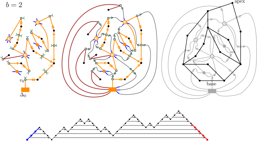
Figure 20: Constructing a $2b$-irreducible $0$-slice from a $b$-decorated tree (here $b=2$). Top left: we first equip the tree with buds attached to bioriented edge-vertices (two buds each, green) and to bent edge-vertices (one bud each). Bottom: the path coding for the sequence of leaflets and buds read counterclockwise around the tree from $\Delta_{0}$ (black steps). The path is (minimally) completed into a Dyck path by adding an initial series of $l=3$ up steps (in blue) and a final series of $l+1=4$ down steps. We also indicated (dark grey arrows) the canonical matching of up and down steps. Top center: we add accordingly a sequence of $l$ leaflets and one of $l+1$ twigs (with buds) attached to $\Delta_{0}$. Each leaflet is then canonically matched to a subsequent bud counterclockwise around the tree by a system of non-crossing arches (in dark grey). Top right: removing the primal edges yields the dual map (in grey) of the desired $0$-slice (in black).

Consider now a descending subtree $\mathcal{T}$ of the decorated tree, which codes for a $2p$-(sub)slice for some $p$ between $0$ and $b$, and which we root at the parent half-edge of $\Delta(BC)$ if the $2p$-slice has base $BC$ (this parent edge is a primal half-edge with $p$ descending arrows if $1\leq p\leq b$ or a dual edge without arrows if $p=0$). We define the charge $c(\mathcal{T})$ of the subtree $\mathcal{T}$ as the total number of incident leaflets minus that of incident buds.

Proposition A.1.

We have

$$c(\mathcal{T})=\left\{\begin{matrix}2p\ \ &\hbox{if\ $1\leq p\leq b$},\\ 1\ \ &\hbox{if\ $p=0$}.\end{matrix}\right.$$ (57)

Proof.

Assume $b>1$. The above property is proved by induction on the three cases that arise:

• (I) $\mathcal{T}$ is a subtree coding for a $2p$-slice with $p<b$, excluding case (III);

• (II) $\mathcal{T}$ is a subtree coding for a $2b$-slice;

• (III) $\mathcal{T}$ is a subtree coding for a $2(b-1)$-slice that is a $2b$-angle.

In case (I), $\Delta(C)$ is an internal vertex of the tree with $q$ descending subtrees coding for $2p_{i}$-slices with $p_{i}\geq 1$ ($1\leq i\leq q$) and $p_{1}+\cdots+p_{q}=(p+1)$. From the induction hypothesis, those contribute a total of $2p_{1}+\cdots+2p_{q}$ to $c(\mathcal{T})$. If $0<p<b$, $\Delta(BC)$ is a bioriented edge-vertex and gives rise to two buds hence contributes $-2$ to $c(\mathcal{T})$, so that $c(\mathcal{T})=2(p_{1}+\cdots+p_{q})-2=2p$ as wanted. If $p=0$, $\Delta(BC)$ is a bent edge-vertex and gives rise to one bud hence contributes $-1$ to $c(\mathcal{T})$, so that $c(\mathcal{T})=2(p_{1}+\cdots+p_{q})-1=2(0+1)-1=1$ as wanted (in fact we necessarily have $q=1$ and $p_{1}=1$ in this case).

In case (II), $\Delta(BC)$ is a bent edge-vertex and contributes $-1$ to $c(\mathcal{T})$. The descending subtree starts with a labeled vertex of degree $2m$ with $m-b-1$ twigs, each contributing $-1$ to $c(\mathcal{T})$ and a total of $m+b$ leaflets or subtrees coding for $0$-slices, each contributing $+1$ (from the induction hypothesis). This leads to $c(\mathcal{T})=-1-(m-b-1)+(m+b)=2b$ as wanted.

In case (III), $\Delta(BC)$ is a bent edge-vertex and contributes $-1$ to $c(\mathcal{T})$. The descending subtree is a single special vertex carrying $2b-1$ leaflets. This leads to $c(\mathcal{T})=-1+2b-1=2(b-1)$ as wanted. This ends the proof for $b>1$.

For $b=1$, the only difference is in case (III) where $\Delta(BC)$ is a dual/dual edge-vertex and contributes $0$ to $c(\mathcal{T})$. The descending subtree is reduced to a special dual vertex with $1$ leaflet, hence $c(\mathcal{T})=0+1=1$ as wanted since the $2$-angle map is a $0$-slice. ∎

The main lesson of the above proposition is that, if we now consider the whole decorated tree coding for a $0$-slice, completed with the dual half-edge connecting $v_{0}$ to $\Delta_{0}$, this tree, when equipped with buds, has charge $+1$ hence has exactly one more incident leaflet than buds. More precisely, reading the sequence of leaflets and buds encountered by going counterclockwise around the tree from $\Delta_{0}$ gives a two-letter word in the alphabet $\{+1,-1\}$ (with the correspondence leaflet $\to+1$ and bud $\to-1$) with one more $+1$ than $-1$. This in turn can be represented as a two-step path with up ($+1$) and down ($-1$) steps, starting from height $0$ and ending at height $+1$. Calling $-l$ the minimum height, with $l\geq 0$, we can transform this path into a Dyck path from height $0$ to height $0$, and staying above or at height $0$, by completing the path with $l$ preceding up steps and $l+1$ following down steps and by shifting the heights by $+l$. Now, as it is well-known for Dyck paths, each ascending step can be matched canonically to a subsequent descending step at the same height on its right (see Figure 20-bottom).

Transposed to the bud-equipped completed decorated tree, this means that, if we further equip it by $l$ leaflets and $l+1$ twigs attached to $\Delta_{0}$ (with a bud attached to each new added twig) and read the sequence of leaflets and buds counterclockwise around the completed tree, there is a canonical matching where each leaflet is connected to a subsequent bud by an arch so that the arch system is non-crossing, does not cross the tree, and no arch passes below $\Delta_{0}$ (see Figure 20, top). These arches reconstruct precisely the missing dual half-edges so that, if we now remove from the tree the primal half-edges (i.e. the half-edge carrying arrows and the primal half-edges in the twigs), and erase all the edge-vertices, we find the dual map of the $0$-slice that we are looking for. The apex of the $0$-slice is dual to the external face while its base is dual to edge of the dual map that contained $v_{0}$ (see Figure 20, top right).

Appendix B Compatibility of formula (1) with Budd’s expression

We start from (1), and express $\alpha_{k,n}^{(b)}$ via (18). This leads to:

$$\begin{split}\mathcal{N}_{n}^{(b)}(2m_{1},\ldots,2m_{n})&=(n-2)![z^{n-2}]\mathcal{S}\\ \hbox{with }\mathcal{S}&=\sum_{k_{1},\ldots,k_{n}\geq 0}p^{(b)}_{k_{1}}(m_{1})q^{(b)}_{k_{2}}(m_{2})\cdots q^{(b)}_{k_{n}}(m_{n})\frac{U_{0}(z)^{1+\sum\limits_{i\geq 1}k_{i}}}{1+\sum\limits_{i\geq 1}k_{i}}\end{split}$$ (58)

We now invert the relation (45) with $c\to b$, namely:

$$p_{k}^{(b)}(m)=\sum_{j=0}^{k}(-1)^{j}\binom{2b+j}{j}q_{k-j}^{(b)}(m)$$ (59)

which leads to:

$$\begin{split}\mathcal{S}&=\sum_{k_{1},\ldots,k_{n}\geq 0}\sum_{j=0}^{k_{1}}(-1)^{j}\binom{2b+j}{j}q^{(b)}_{k_{1}-j}(m_{1})q^{(b)}_{k_{2}}(m_{2})\cdots q^{(b)}_{k_{n}}(m_{n})\frac{U_{0}(z)^{1+\sum\limits_{i\geq 1}k_{i}}}{1+\sum\limits_{i\geq 1}k_{i}}\\ &=\sum_{k_{0},k_{1},\ldots,k_{n}\geq 0}(-1)^{k_{0}}\binom{2b+k_{0}}{k_{0}}q^{(b)}_{k_{1}}(m_{1})\cdots q^{(b)}_{k_{n}}(m_{n})\frac{U_{0}(z)^{k_{0}+1+\sum\limits_{i\geq 1}k_{i}}}{k_{0}+1+\sum\limits_{i\geq 1}k_{i}}\end{split}$$ (60)

through renaming $(j,k_{1})\to(k_{0},k_{0}+k_{1})$. We now deduce:

$$\begin{split}\mathcal{S}&=\int_{0}^{U_{0}(z)}dr\sum_{k_{0},k_{1},\ldots,k_{n}\geq 0}(-1)^{k_{0}}\binom{2b+k_{0}}{k_{0}}r^{k_{0}+\sum\limits_{i\geq 1}k_{i}}q^{(b)}_{k_{1}}(m_{1})\cdots q^{(b)}_{k_{n}}(m_{n})\\ &=\int_{0}^{U_{0}(z)}\frac{dr}{(1+r)^{2b+1}}\sum_{k_{1},\ldots,k_{n}\geq 0}r^{\sum\limits_{i\geq 1}k_{i}}q^{(b)}_{k_{1}}(m_{1})\cdots q^{(b)}_{k_{n}}(m_{n})\\ &=\int_{0}^{U_{0}(z)}\frac{dr}{(1+r)^{2b+1}}\prod_{i=1}^{n}I(b,m_{i};r)\end{split}$$ (61)

with $I(b,m;r):=\sum_{k=0}^{+\infty}r^{k}q^{(b)}_{k}(m)$ as in [Bud22, Equation (48)]. This reproduces precisely the result of [op. cit., Equation (66)] upon identifying this reference’s $J^{-1}(b;z)$ to our $U_{0}(z)$: indeed, recall from (28) that $U_{0}(z)$ is determined implicitly by $z=h_{b}(U_{0}(z))$, and note that our $h_{b}(u)$ is the same as $J(b;u)$ as defined in [op. cit., Equation (49)].

Appendix C Counting planar $2b$-irreducible $2b$-angulations with $n$ faces

In this appendix, we consider the problem of counting planar $2b$-irreducible $2b$-angulations, that is $2b$-irreducible maps whose all faces have degree $2b$. Note that such maps are automatically bipartite and tight. We noted after Theorem 1.1 that it does not quite hold in the case where all $m_{i}$ are equal to $b$, for there is an pathological term as visible in [Bud22, Theorem 1]. Precisely, we have the following:

Proposition C.1.

For any $n\geq 3$, the number of $2b$-irreducible $2b$-angulations with $n$ labeled faces is equal to

$$\mathcal{N}_{0,n}^{(b)}(\underbrace{2b,\ldots,2b}_{n\text{ times}})=(n-3)!\sum_{k=0}^{n-3}(-1)^{k}\binom{2b+k}{k}\alpha_{k,n-3}^{(b)}+\mathbf{1}_{n\geq 4}\frac{(n-1)!}{2}(-1)^{n}.$$ (62)

Let us observe that the first term in the right-hand side is equal to the right-hand side of (1) for $m_{1}=\cdots=m_{n}=b$, since $p_{k}^{(b)}(b)=(-1)^{k}\binom{2b+k}{k}$ and $q_{k}^{(b)}(b)=\delta_{k,0}$. Here it is slightly puzzling that the sign alternates with $k$, whereas under the assumptions of Theorem 1.1 all the terms in (1) were non-negative. In the remainder of this appendix, we give a combinatorial, but unfortunately not bijective, derivation of Proposition C.1. It is based on an argument which was mentioned, but not detailed, at the end of [BG14, Section 9.3].

The bijection described in Section 2.1 does not easily allow to count $2b$-irreducible $2b$-angulations: in the two items characterizing $2b$-irreducible maps at the end of Proposition 2.3, it is always assumed that face $1$ has a degree strictly larger than $b$. To circumvent this issue, we first count closely related objects by specializing Proposition 3.18 to the case $c=b-1$, $m_{1}=\ldots=m_{n}=b$: noting that, by (43), we have $p_{k}^{(b-1)}(b,b)=q_{k}^{(b-1)}(b)=\binom{2b-1}{k}$, we obtain the following:

Lemma C.2.

For any $n\geq 3$, the number of essentially $2b$-irreducible $2b$-angulations with $n$ labeled faces with separating girth equal to $2b$ is equal to

$$\beta^{(b)}_{n}:=(n-3)!\sum_{k\geq 0}\binom{2b-1}{k}\alpha^{(b)}_{k,n-3}.$$ (63)

Note that, by (18), we have

$$\sum_{n\geq 3}\frac{\beta^{(b)}_{n}}{(n-3)!}z^{n-3}=\sum_{k\geq 0}\binom{2b-1}{k}U_{0}^{\prime}(z)U_{0}(z)^{k}=U_{0}^{\prime}(z)(1+U_{0}(z))^{2b-1}$$ (64)

with $U_{0}(z)$ as in Section 3.1.2 (recall that it depends implicitly on $b$). Integrating over $z$ and multiplying by $2b$, we deduce that $(1+U_{0}(z))^{2b}$ is the generating function of essentially $2b$-irreducible $2b$-angulations with two marked faces $1$ and $2$, such that face $1$ is rooted and such that the separating girth is equal to $2b$, counted with a weight $z$ per unmarked face. In what follows, we denote the set of such maps by $\mathfrak{M}_{b}$, and by $\mathfrak{N}_{b}$ its subset consisting of maps which are $2b$-irreducible in the strong (not just essentially) sense, which means that the only separating cycles of length $2b$ are the contours of the marked faces. The following lemma corresponds to [BG14, Equation (9.21)] specialized to the case of $2b$-angulations:

Lemma C.3.

Let us denote by $N_{b}(z)$ the generating function of maps in $\mathfrak{N}_{b}$, counted with a weight $z$ per unmarked face. Then, we have

$$(1+U_{0}(z))^{2b}=\frac{1}{1-\left(N_{b}(z)-1-2bz\right)-b\frac{2z+z^{2}}{1+2z+z^{2}}}.$$ (65)

Proof.

Let $\mathbf{m}$ be a map in $\mathfrak{M}_{b}$, i.e. a map contributing to $(1+U_{0}(z))^{2b}$, which we draw in the complex plane with the face $1$ containing the origin and the face $2$ chosen as the outer face. Let $C$ be the set of separating cycles of $\mathbf{m}$ with length $2b$. We say that a cycle $c\in C$ is cuttable if it does not intersect any other cycle $c^{\prime}\in C$, that is $c^{\prime}$ remains within one of the two closed regions delimited by $c$. Upon cutting $\mathbf{m}$ along all cuttable cycles, we decompose it into a sequence of maps $(\mathbf{m}_{1},\ldots,\mathbf{m}_{\ell})$ nested into one another. These maps belong also to $\mathfrak{M}_{b}$, since they have naturally two marked faces and may be rooted in some canonical manner. All of them have at least one unmarked face.

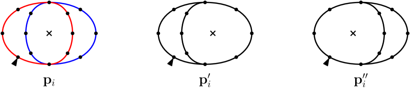
Figure 21: The pathological maps $\mathbf{p}_{i}$, $\mathbf{p}^{\prime}_{i}$ and $\mathbf{p}^{\prime\prime}_{i}$, $i=1,\ldots,b$, in $\mathfrak{M}_{b}$ (here $b=4$ and $i=1$). The arrow indicates the root and the cross the marked inner face. In $\mathbf{p}_{i}$, there are two minimal separating cycles (shown in red and blue) which intersect each other, hence are not cuttable. The maps $\mathbf{p}^{\prime}_{i}$ and $\mathbf{p}^{\prime\prime}_{i}$ contain no uncuttable cycles, but they are still pathological in the sense that, when cutting a map in $\mathfrak{M}_{b}$ along its cuttable cycles (as explained in the text) then we cannot find two consecutive elements $\mathbf{p}_{i},\mathbf{p}^{\prime}_{i},\mathbf{p}^{\prime\prime}_{i}$ with the same index $i$.

Now, we observe that for each $\mathbf{m}_{j}$, two situations may arise: either it contains no minimal separating cycle other than the contours of the marked faces, in which case it belongs to $\mathfrak{N}_{b}$, or it contains such a cycle, which necessarily intersects another minimal separating cycle as it would have been cuttable otherwise. In that case, using the essential $2b$-irreducibility, we see that $\mathbf{m}_{j}$ necessarily coincides with the “pathological” map $\mathbf{p}_{i}$ displayed on Figure 21 for some $i=1,\ldots,b$ (this index indicates the position of the root corner).

We note that there is an extra constraint on the sequence $(\mathbf{m}_{1},\ldots,\mathbf{m}_{\ell})$: let $\mathbf{p}^{\prime}_{i}$ and $\mathbf{p}^{\prime\prime}_{i}$ be the other “pathological” maps displayed on Figure 21. While they belong to $\mathfrak{N}_{b}$, it is not possible to have within the sequence $(\mathbf{m}_{1},\ldots,\mathbf{m}_{\ell})$ two consecutive elements equal to $\mathbf{p}_{i}$, $\mathbf{p}^{\prime}_{i}$ or $\mathbf{p}^{\prime\prime}_{i}$ with the same index $i$ (otherwise we would have either cut $\mathbf{m}$ along an uncuttable cycle, or have in $\mathbf{m}$ a cycle of length $2b$ which is neither separating nor the contour of a face).

We may code for this constraint in the following way: to the sequence $(\mathbf{m}_{1},\ldots,\mathbf{m}_{\ell})$ we associate a word $w$ of length $\ell$ over the alphabet $\{O,P_{1},\ldots,P_{b}\}$, by replacing each $\mathbf{m}_{j}$ equal to $\mathbf{p}_{i}$, $\mathbf{p}^{\prime}_{i}$ or $\mathbf{p}^{\prime\prime}_{i}$ for some $i$ by the letter $P_{i}$, and all other $\mathbf{m}_{j}$’s by the letter $O$. The word $w$ is such that two letters $P_{i}$ with the same index cannot appear consecutively. Splitting $w$ at each occurrence of $O$, it may be decomposed as $w_{0}Ow_{1}O\cdots Ow_{k}$ for some $k\geq 0$ where $w_{0},\ldots,w_{k}$ are so-called Smirnov words [FS09, Example III.24], and have the multivariate generating function

$$S(v_{1},\ldots,v_{b})=\left(1-\sum_{i=1}^{b}\frac{v_{i}}{1+v_{i}}\right)^{-1}$$ (66)

where $v_{i}$ is the weight per occurrence of the letter $P_{i}$. Attaching a weight $u$ per occurrence of $O$, we deduce that the generating function of the words $w$ of the wanted form is equal to

$$\sum_{k\geq 0}S(v_{1},\ldots,v_{b})^{k+1}u^{k}=\frac{S(v_{1},\ldots,v_{b})}{1-uS(v_{1},\ldots,v_{b})}=\frac{1}{1-u-\sum_{i=1}^{b}\frac{v_{i}}{1+v_{i}}}.$$ (67)

The generating function of the sequences $(\mathbf{m}_{1},\ldots,\mathbf{m}_{\ell})$ obeying our constraint is then obtained by substituting $u=N_{b}(z)-1-2bz$ (corresponding to the generating function of maps in $\mathfrak{N}_{b}$ having at least one unmarked face and different from $\mathbf{p}^{\prime}_{1},\mathbf{p}^{\prime\prime}_{1},\ldots,\mathbf{p}^{\prime}_{b},\mathbf{p}^{\prime\prime}_{b}$) and, for all $i=1,\ldots,b$, $v_{i}=2z+z^{2}$ (corresponding to the combined weights of $\mathbf{p}_{i},\mathbf{p}^{\prime}_{i},\mathbf{p}^{\prime\prime}_{i}$). This yields the right-hand side of (65), and we may conclude by verifying that the mapping $\mathbf{m}\mapsto(\mathbf{m}_{1},\ldots,\mathbf{m}_{\ell})$ is a bijection. ∎

End of the proof of Proposition C.1.

By Lemma C.3, we have

$$\begin{split}N_{b}(z)&=2-(1+U_{0}(z))^{-2b}+2bz-b\frac{2z+z^{2}}{1+2z+z^{2}}\\ &=1-\sum_{i\geq 1}(-1)^{i}\binom{2b-1+i}{i}U_{0}(z)^{i}+b\frac{z^{2}(3+2z)}{(1+z)^{2}}.\end{split}$$ (68)

Extracting the coefficient of $z^{n-2}$ for $n\geq 3$ and using (18), we get

$$\begin{split}[z^{n-2}]N_{b}(z)&=\sum_{i\geq 1}(-1)^{i-1}\binom{2b+i-1}{i}\frac{i}{n-2}\alpha_{i-1,n-3}+b(-1)^{n}(n-1)\mathbf{1}_{n\geq 4}\\ &=\frac{2b}{n-2}\sum_{k\geq 0}(-1)^{k}\binom{2b+k}{k}\alpha_{k,n-3}+b(-1)^{n}(n-1)\mathbf{1}_{n\geq 4}.\end{split}$$ (69)

We obtain the wanted expression (62) by multiplying by $(n-2)!$ to label the $n-2$ unmarked faces, and dividing by $2b$ to remove the rooting of face $1$. ∎

References

- [AP15] Marie Albenque and Dominique Poulalhon “A generic method for bijections between blossoming trees and planar maps” In Electron. J. Combin. 22.2, 2015, pp. Paper 2.38\bibrangessep44 DOI: 10.37236/3386
- [BF12] Olivier Bernardi and Éric Fusy “A bijection for triangulations, quadrangulations, pentagulations, etc.” In Journal of Combinatorial Theory, Series A 119.1, 2012, pp. 218–244 DOI: 10.1016/j.jcta.2011.08.006
- [BF12a] Olivier Bernardi and Éric Fusy “Unified bijections for maps with prescribed degrees and girth” In Journal of Combinatorial Theory, Series A 119.6, 2012, pp. 1351–1387 DOI: 10.1016/j.jcta.2012.03.007
- [BFL23] Olivier Bernardi, Éric Fusy and Shizhe Liang “Grand Schnyder Woods”, 2023 arXiv:2303.15630 [math.CO]
- [BG14] J. Bouttier and E. Guitter “On irreducible maps and slices” In Combin. Probab. Comput. 23.6, 2014, pp. 914–972 DOI: 10.1017/S0963548314000340
- [BG14a] J. Bouttier and E. Guitter “A note on irreducible maps with several boundaries” In Electron. J. Combin. 21.1, 2014, pp. Paper 1.23\bibrangessep18 DOI: 10.37236/3443
- [BGM24] Jérémie Bouttier, Emmanuel Guitter and Grégory Miermont “Enumeration of maps with tight boundaries and the Zhukovsky transformation”, 2024 arXiv:2406.13528 [math.CO]
- [BGM24a] Jérémie Bouttier, Emmanuel Guitter and Grégory Miermont “On quasi-polynomials counting planar tight maps” In Combinatorial Theory 4.1, 2024 DOI: 10.5070/C64163849
- [Bud22] Timothy Budd “On polynomials counting essentially irreducible maps” In The Electronic Journal of Combinatorics 29.2, 2022, pp. research paper p2.45\bibrangessep43 DOI: 10.37236/9746
- [Bud22a] Timothy Budd “Irreducible metric maps and Weil-Petersson volumes” In Communications in Mathematical Physics 394.2, 2022, pp. 887–917 DOI: 10.1007/s00220-022-04418-6
- [FS09] Philippe Flajolet and Robert Sedgewick “Analytic combinatorics” Available online at http://algo.inria.fr/flajolet/Publications/books.html. Cambridge University Press, Cambridge, 2009, pp. xiv+810 DOI: 10.1017/CBO9780511801655
- [FSP08] Éric Fusy, Gilles Schaeffer and Dominique Poulalhon “Dissections, orientations, and trees with applications to optimal mesh encoding and random sampling” In ACM Trans. Algorithms 4.2 New York, NY, USA: Association for Computing Machinery, 2008 DOI: 10.1145/1361192.1361196
- [MS68] R.C. Mullin and P.J. Schellenberg “The enumeration of c-nets via quadrangulations” In Journal of Combinatorial Theory 4.3, 1968, pp. 259–276 DOI: 10.1016/S0021-9800(68)80007-9
- [Nor10] Paul Norbury “Counting lattice points in the moduli space of curves” In Mathematical Research Letters 17.3 International Press of Boston, Somerville, MA, 2010, pp. 467–481 DOI: 10.4310/MRL.2010.v17.n3.a7
- [Nor13] Paul Norbury “String and dilaton equations for counting lattice points in the moduli space of curves” In Transactions of the American Mathematical Society 365.4, 2013, pp. 1687–1709 URL: https://www.jstor.org/stable/23513423
- [Sch15] Gilles Schaeffer “Planar maps” In Handbook of enumerative combinatorics, Discrete Math. Appl. (Boca Raton) CRC Press, Boca Raton, FL, 2015, pp. 335–395 URL: https://www.lix.polytechnique.fr/~schaeffe/Biblio/HB.pdf
- [Tut62] W.. Tutte “A Census of Slicings” In Canadian Journal of Mathematics 14, 1962, pp. 708–722 DOI: 10.4153/CJM-1962-061-1