Measurement of the electric field distribution in streamer discharges

Abstract

Using electric field induced second harmonic generation (E-FISH), we performed direction-resolved absolute electric field measurements on single-channel streamer discharges in 70 mbar (7 kPa) air with 0.2 mm and 2 ns resolutions. In order to obtain the absolute (local) electric field, we developed a deconvolution method taking into account the phase variations of E-FISH. The acquired field distribution shows good agreement with the simulation results under the same conditions, in direction, magnitude and in shape. This is the first time that E-FISH is applied to streamers of this size (>0.5 cm radius), crossing a large gap. Achieving these high resolution electric field measurements benefits further understanding of streamer discharges and enables future use of E-FISH on cylindrically symmetric (transient) electric field distributions.

Streamer discharges are fast propagating ionization fronts that appear as the precursor to lightning leaders and as sprites in nature [1]. The electric field is the driving force behind streamers and determines their energy transfer and chemical activity [2]. There are various studies focusing on electric field measurement of discharges using different diagnostics, including electric-field-induced coherent anti-Stokes Raman scattering (E-CARS) [3] and Stark spectroscopy [4]; while methods for measuring the electric field in streamers, which are highly transient, are limited, and if present, have very low temporal and spatial resolution. Most recently, Dijcks et al. [5] determined the electric field of single-channel streamers in pure nitrogen and synthetic air at pressures of 33 mbar by using optical emission spectroscopy (OES). However, this method has the disadvantages that it depends on light emission, cannot measure the field direction and has a rather low spatial and temporal resolution. The lack of suitable methods hinders further understanding of streamers and other transient discharges driven by the electric field.

To tackle these problems, a new technique called electric field induced second harmonic generation (E-FISH) has been introduced to the plasma community to measure the electric field of various kinds of plasmas [6, 7]. In this method, a high power laser beam non-linearly interacts with an electric field in a gas, generating second harmonics. The intensity of these second harmonics scales directly with the square of the electric field strength, and the polarization direction aligns with the field orientation. Initially, this method was considered easy to implement and the measured signals straightforward to interpret. However, it has been shown that the measured signals are strongly related to the laser beam profile, and depend heavily on the electric field profile and not just its integrated value due to phase variations along the laser beam [8]. A solution has been proposed in [9], but uniformity of the electric field in one of the directions perpendicular to the laser beam is assumed, which is not a valid assumption for streamers.

In this Letter, for the first time, we report detailed direction-resolved measurements of the electric field distribution in single-channel streamers in air by using E-FISH. The electric field is restored from the E-FISH signals by applying a deconvolution method including all phase variations, where cylindrical symmetry is assumed. Also, light emission from the discharge is captured. Next to this, simulations on the electric field and the emission spectrum of the second positive system (SPS) of N₂ are obtained using a 2D axisymmetric drift-diffusion-reaction fluid model [10] of the streamers under the same conditions. Li et al. [10] have shown that this model is very reliable in simulating streamers in air; its calculated streamers closely match in velocities and diameters with experimental results.

The experimental results show a tremendous improvement in resolution compared to previous work. Thus far, such detailed electric field distributions of transient plasmas could only be obtained through simulations. Moreover, we reveal the electric field in areas with little to no light emission, which contains the most valuable information for streamer discharges. The magnitude, shape and direction of the field and its position relative to the light emission are in agreement with the simulations. This enables further understanding of streamers and empowers future use of E-FISH.

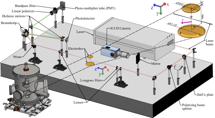
Figure 1: A render of the E-FISH setup. The vacuum vessel is excluded from the main image for clarity and is instead shown on the bottom left. We use a coordinate system in which the streamer propagates in the $y$ direction, the laser beam is along the $z$ direction, and the radial coordinate is given by $r=\sqrt{x^{2}+z^{2}}$. The detailed geometry of the electrodes including streamer, $r$-direction definition, and the laser beam (dimensions in mm) is shown on the top right.

A schematic of the experimental setup is shown in Fig. 1. In short, a 100 mJ Nd:YAG laser (EKSPLA SL234-10-G-SH) beam with a pulse width of 120 ps at 1064 nm is focused into the discharge area by an $f=500$ mm lens. The beam waist and Rayleigh length $z_{R}$ are measured to be 0.13 mm and 12 mm, respectively, by using the knife edge method [11]. Two longpass filters remove any second harmonic light generated by the laser itself and by interaction between the laser beam and the upstream optics. Second harmonic light is generated when the laser interacts with the electric field in the streamers that are produced inside a vessel. The fundamental and second harmonic beams are collimated again by another $f=500$ mm lens. These two colinear beams are then fully separated by using a prism and three dichroic mirrors. The fundamental beam intensity is measured by a photodetector (Thorlabs DET36A/M). The second harmonic beam is directed to a photomultiplier (PMT, Hamamatsu H6779-04), with a bandpass filter attached in front of it to filter out any stray light. To increase the signal-to-noise ratio, the laser beam is polarized parallel to the to-be-measured electric field direction by using a half-wave plate and a polarizer, because the second harmonic generation process has a higher efficiency under this configuration [7]. A polarizer is positioned in front of the PMT to measure the vector components of the electric field.
To generate streamers, we use the setup that has been described in [5]. The high voltage pulses are generated by a pulsed power circuit (Belhke HTS) with an amplitude of 9.5 kV, a rise time of about 50 ns, a voltage jitter of $\sim$1 ns, and a duration of 400 ns at a repetition rate of 60 Hz. The electrodes are protrusion-to-plane electrodes, where the high voltage electrode contains a 10 mm protruding pin in the center (1 mm diameter, 60^∘ tip angle, and 50 µm tip radius). The pin-to-plate gap is 90 mm. The laser beam is at the height of 5.3 cm from the grounded bottom plate electrode. During the experiment, the vessel is continuously flushed with dry air with a flow rate of 2 L/min and the pressure is fixed at 70 mbar (7 kPa). The pulse repetition rate, the dedicated electrode geometry, and the reduced pressure ensure the high repetitiveness in both time and space of the single positive streamers, and thus the quality of the E-FISH signals.
The moment the laser interacts with the streamer electric field, the discharge image is captured by an ICCD camera (Andor DH334T) with a gating time of 2 ns. From these images, only a horizontal strip at the height of the laser beam is used. Under the above mentioned conditions, the streamer propagation velocity is measured to be 3.5$\times 10^{5}$ m/s. The laser, the high voltage pulses, and the gating of the ICCD camera are synchronized by a digital delay generator.
In order to obtain the electric field at different positions in the discharge, the entire vessel is fixed on a translation stage such that it can move over the horizontal axis (coordinate $x$) perpendicular to the laser beam direction (coordinate $z$). The second dimension is acquired by varying the delay between the high voltage pulse (and consequently streamer inception) and the laser trigger. This allows us to generate an image with time as one dimension and the horizontal cross-section of the streamer in the second dimension both for optical emission and electric field strength. Because the single-channel streamers under investigation are roughly constant in shape and velocity when traversing the center of the electrode gap [10], the time axis is very similar to the streamer propagation direction axis (coordinate $y$). For a single measurement of one field direction, a time range of $-$80 to 120 ns with a step size of 2 ns and a spatial range of $-$15 to 15 mm with a step size of 0.2 mm is used, where $t=0$ is defined as the moment when the electric field in the $y$-direction peaks, and $x=0$ the middle of the streamer in the $x$-direction . For every delay and position, 40 laser shots are recorded, resulting in one measurement consisting of more than 400,000 laser shots (the grid size is coarser for the lower field region). A full measurement, for both directions of the electric field, takes about 15 hours.

The signal we measure is $s(x,t)=\sqrt{I_{2\omega}/I_{\omega}^{2}}$, where $I_{2\omega}$ and $I_{\omega}$ represent the intensity of the second harmonic and fundamental beams, respectively. This signal is the result of a line-of-sight integration along the laser propagating direction [12, 8]:

$$s(x,t)=C_{\mathrm{cal}}\left|\int_{-L}^{L}\frac{e^{-i\Delta kz}}{1+i\frac{z}{z_{R}}}E_{\mathrm{ext}}(x,z,t)\,\mathrm{d}z\right|,$$ (1)

where $C_{\mathrm{cal}}$ is a calibration constant; ${\leavevmode 2}L$ is the interaction length of the laser beam and the electric field; $\Delta k$ is the wavevector mismatch between the fundamental and second harmonic wavelengths, $z_{R}$ is the Rayleigh length of the focused beam, and $E_{\mathrm{ext}}$ the external, to-be-measured electric field of which the $x$- and $y$-component can be measured. $\Delta k$ is 3.45 m^-1 for 70 mbar air with a 1064 nm input beam [13]. The complex denominator, $1+i\frac{z}{z_{R}}$, introduces an extra phase shift $\mathrm{tan^{-1}}\frac{z}{z_{R}}$ called Gouy phase, which originates from the focused Gaussian beam shape. For an axisymmetric streamer, the electric field in the $y$-direction $E_{y}$ will also be axisymmetric, such that $E_{\mathrm{ext}}(x,z,{\leavevmode t})=E_{y}(r,{\leavevmode t})$ where $r=\sqrt{x^{2}+z^{2}}$. We can also make use of the axisymmetry when measuring the field in the $x$-direction $E_{x}$, by expressing it as $E_{x}=\sin(\theta)E_{r}$, where $E_{r}$ is the axisymmetric radial component and $\sin(\theta)=x/r$. In this case, we thus have $E_{\mathrm{ext}}(x,z,{\leavevmode t})=x/r\,E_{r}(r,{\leavevmode t})$.

We cannot use a standard inverse Abel transform to solve equation (1). Instead, we approximate the integral by a weighted sum over samples $E_{y}(r_{i})$ or $E_{r}(r_{i})$, at a given set of radial coordinates. Given a set of measurements $s(x_{j})$, we can then solve an approximately linear system to obtain $E_{x}(r_{i})$ or $E_{y}(r_{i})$. We include a small regularization parameter in this procedure to make the inversion unique and robust to noise in the measurements. A detailed description of the inversion procedure is given in the supplementary material [14]. Similarly, the optical emission is Abel-inverted.

To obtain the absolute field strength, a calibration measurement on a known field distribution is performed. We designed rod-to-rod and rod-to-cylinder electrodes for the calibration of $E_{y}$ and $E_{x}$, respectively, which generate an electric field with a similar shape as the streamer. First, the electrostatic field of these configurations is simulated in COMSOL Multiphysics. Then the field is forward-transformed by using the inverse of the algorithm described above to obtain the “calculated E-FISH  signals”. The ratio between the calculated signals and the measured signals leads to the calibration constant $C_{\mathrm{cal}}$.

Figure 2 shows the amplitudes of the E-FISH signals for $E_{y}$ and $E_{x}$ of a single-channel streamer in 70 mbar air with an applied voltage of 9.5 kV. It is worth noting that the distribution of the $E_{x}$ signals can become asymmetric around $r=0$ due to interference between the E-FISH signal and the background signal. We discuss this issue, its implications on other E-FISH results and corresponding solutions in detail in the supplementary material [14].

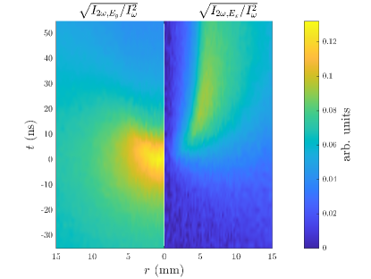
Figure 2: Measured E-FISH signals for $E_{y}$ (left) and $E_{x}$ (right) of a streamer in 70 mbar air with an applied voltage of 9.5 kV. $t=0$ is defined as the time when $E_{y}$ peaks.

By using the deconvolution method described, and multiplying with calibration constant $C_{\mathrm{cal}}$, the absolute values of both the $r$ and $y$ components of the electric field can be restored from the signals. The magnitude of the electric field is calculated as $\lvert E\rvert=\sqrt{E_{r}^{2}+E_{y}^{2}}$. Figure 3 shows the comparison of local light emission intensity and electric field distribution between experiment and simulation results. $\lvert E\rvert/N$ is the absolute reduced electric field in Townsend (Td, $E/N$ in units $10^{-21}$ V$\cdot$m²), where $N$ is the gas number density. Here, $N$ equals $1.88\cdot 10^{24}$ m^-3 at 70 mbar when assuming room temperature. In the simulation, the conditions in [10] are adapted to fit the voltage and pressure used in this experiment. The emitted light is estimated by the $\mathrm{N_{2}(C^{3}\Pi_{u})}$ density because the SPS transition is responsible for most of the optical emission under our discharge conditions [15]. Note that the simulation only treats one voltage pulse, therefore the heating effect of repetitive pulses is not taken into account. In the experiments the gas temperature will likely be elevated above room temperature [16, 17], but its exact value cannot be determined in this setup.

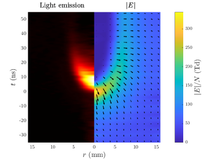
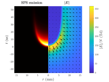
Figure 3: Experimental (top) and simulation (bottom) results of local normalized light emission intensity and reduced electric field distribution.

Qualitatively, the experimental and simulation results exhibit very high visual similarity. In both cases the space charge layer with the crescent shape of the streamer head is clearly visible. The electric field is most intense around the head of streamers and mostly pointing downwards. Inside the streamer channel, the electric field almost vanishes, as the highly conductive streamer channel shields the electric field very efficiently. Furthermore, the light emission always lags behind the electric field [18, 19]. Thus, light emission based methods to measure the electric field can only determine the field in the area behind the peak electric field, while E-FISH can resolve the field distribution completely. In the simulation, the light emission profile shows a sharp front, while in the experiment it is smeared out more and shows some internal structure. The smearing is partly due to the camera integration time and streamer jitter, while the internal structure is attributed to oscillating ripples in the voltage waveform that change the velocity of the streamers.
Quantitatively, the streamers in both cases have similar size and very close field magnitude. The electrodynamic diameter measured by the electric field is defined as the radial position at which $E_{r}$ reaches a maximum. In experiment and simulation these are 7.4 mm and 7.8 mm respectively for $t=50\,$ns, which agrees very well.

Figure 4 shows a comparison of the axial field evolution and light emission, and of the radial field and light emission at 50 ns between experiment and simulation.

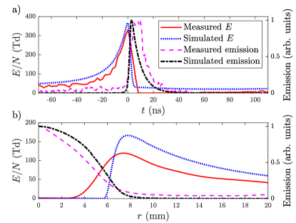
Figure 4: A comparison of a) the axial field ($E_{y}$) and light emission and b) the radial field ($E_{r}$) and light emission between E-FISH experiment and simulation. The radial field was determined at 50 ns while the radial light emission was integrated over the entire time domain and normalized to its maximum.

In figure 4(a), it is shown that the simulated and measured electric field stay roughly constant at the background field level and rise rapidly at around $t=-20$ ns when the streamer head is approaching the probing laser. The maximum electric field peaks at 364 Td and 320 Td for simulation and experiment, respectively. These values correspond to $6.4\cdot 10^{5}$ V/m and $5.6\cdot 10^{5}$ V/m respectively. The difference between experiment and simulation is likely caused by the temporal resolution of the experiment being limited by the streamer jitter and by a slightly elevated gas temperature in the experiments.

Subsequently, the axial field drops drastically within 5 ns and remains at almost zero, as the streamer leaves behind a conducting channel after the streamer head crosses. The peak value is higher than the breakdown threshold in air ($\sim$120 Td) and is lower than the field determined by OES in [5] with a peak field of 540 Td in 33 mbar air and in [19] around 500 Td at atmospheric pressure. Mrkvic̆ková et al. [20] compared the electric field in an atmospheric pressure Townsend discharge in nitrogen determined by E-FISH and OES, and found that the OES method gives systematically higher values. They attributed this to the omission of additional population processes of $\mathrm{N_{2}^{+}(B^{2}\Sigma_{u}^{+})}$. In figure 4(b), the radial field profiles have similar shapes, except that the measured field has a smoother edge and lower peak value. This is probably due to the lower field intensity of the calibration measurement as well as a larger background signal of $E_{x}$, which results in a lower sensitivity. Outside the streamer channel, the radial fields in both cases decay with approximately the same speed.

In conclusion, we have used E-FISH to determine for the first time an experimentally obtained detailed direction-resolved spatiotemporal distribution of the electric field in a single-channel streamer. Moreover, the electric field in areas with little to no light emission is revealed. The measurement was performed in 70 mbar air with resolutions of 0.2 mm and 2 ns. Simultaneously, the optical emission was tracked with a resolution of 2 ns. We developed a deconvolution method for E-FISH including the effect of phase variations and designed dedicated calibration experiments for cylindrically symmetrical fields to restore the absolute electric field distribution from E-FISH signals. Simulations on the electric field and SPS emission of the same streamer were obtained using a 2D axisymmetric drift-diffusion-reaction fluid model. We compared the experimental and simulation results and they show great agreement both qualitatively and quantitatively. The maximum electric field peaks at 364 Td and 320 Td for simulation and experiment, respectively. This enables us to further verify and validate the simulation models and have a comprehensive understanding of streamer discharges in nearly all gas mixtures, both on the development and on the chemical processes inside.

It must be noted that for our discharge geometry and laser set-up, the difference in outcome between our full processing method and a more standard Abel inversion, for $E_{y}$ is below 20%. However, the standard Abel inversion is more sensitive to noise from the outer regions and therefore requires more smoothing. For $E_{r}$, a standard Abel inversion is insufficient, as it cannot translate the $E_{x}$ vector into $E_{r}$.

The developed method for analysing E-FISH measurements can be applied on highly repetitive plasmas/electric fields as a scan of the electric field is required. However, cylindrical symmetry is needed.
Future efforts should be directed to adjusting the analysis and corresponding methods to make E-FISH suitable for asymmetric fields. This will allow for high resolution direct electric field measurements of transient/fast moving electric fields in (ionized) gases, which is currently impossible.

Y G was supported by the China Scholarship Council (CSC) Grant No. 202006280041.

References

- Nijdam et al. [2020] S. Nijdam, J. Teunissen, and U. Ebert, Plasma Sources Science and Technology 29, 103001 (2020).
- Patnaik et al. [2017] A. K. Patnaik, I. Adamovich, J. R. Gord, and S. Roy, Plasma Sources Science and Technology 26, 103001 (2017).
- van der Schans et al. [2017] M. van der Schans, P. Böhm, J. Teunissen, S. Nijdam, W. IJzerman, and U. Czarnetzki, Plasma Sources Science and Technology 26, 115006 (2017).
- Cvetanović et al. [2015] N. Cvetanović, M. M. Martinović, B. M. Obradović, and M. M. Kuraica, Journal of Physics D: Applied Physics 48, 205201 (2015).
- Dijcks et al. [2023] S. Dijcks, L. Kusýn, J. Janssen, P. Bílek, S. Nijdam, and T. Hoder, Frontiers in Physics 11, 10.3389/fphy.2023.1120284 (2023).
- Dogariu et al. [2017] A. Dogariu, B. M. Goldberg, S. O’Byrne, and R. B. Miles, Physical Review Applied 7, 024024 (2017).
- Chng et al. [2020a] T. L. Chng, M. Naphade, B. M. Goldberg, I. V. Adamovich, and S. M. Starikovskaia, Optics Letters 45, 1942 (2020a).
- Chng et al. [2020b] T. L. Chng, S. M. Starikovskaia, and M.-C. Schanne-Klein, Plasma Sources Science and Technology 29, 125002 (2020b).
- Nakamura et al. [2021] S. Nakamura, M. Sato, T. Fujii, A. Kumada, and Y. Oishi, Physical Review A 104, 053511 (2021).
- Li et al. [2021] X. Li, S. Dijcks, S. Nijdam, A. Sun, U. Ebert, and J. Teunissen, Plasma Sources Science and Technology 30, 095002 (2021).
- Khosrofian and Garetz [1983] J. M. Khosrofian and B. A. Garetz, Applied Optics 22, 3406 (1983).
- Boyd [2020] R. W. Boyd, Nonlinear optics, fourth edition ed. (Elsevier, AP Academic Press, London, 2020).
- Börzsönyi et al. [2008] A. Börzsönyi, Z. Heiner, M. P. Kalashnikov, A. P. Kovács, and K. Osvay, Applied Optics 47, 4856 (2008).
- [14] See Supplementary Material at [URL will be inserted by publisher] for details on the inversion procedure, calibraion method, and interference issue, which includes Refs. [21, 22].
- Pancheshnyi et al. [2000] S. V. Pancheshnyi, S. V. Sobakin, S. M. Starikovskaya, and A. Y. Starikovskii, Plasma Physics Reports 26, 1054 (2000).
- Adams et al. [2019] S. Adams, J. Miles, T. Ombrello, R. Brayfield, and J. Lefkowitz, Journal of Physics D: Applied Physics 52, 355203 (2019).
- Pai et al. [2010] D. Z. Pai, D. A. Lacoste, and C. O. Laux, Journal of Applied Physics 107, 10.1063/1.3309758 (2010).
- Wagenaars et al. [2007] E. Wagenaars, M. D. Bowden, and G. M. W. Kroesen, Physical Review Letters 98, 075002 (2007).
- Hoder et al. [2015] T. Hoder, Z. Bonaventura, A. Bourdon, and M. Šimek, Journal of Applied Physics 117, 10.1063/1.4913215 (2015).
- Mrkvičková et al. [2023] M. Mrkvičková, L. Kuthanová, P. Bílek, A. Obrusník, Z. Navrátil, P. Dvořák, I. Adamovich, M. Šimek, and T. Hoder, Plasma Sources Science and Technology 32, 065009 (2023).
- Raskar et al. [2022] S. Raskar, K. Orr, I. V. Adamovich, T. L. Chng, and S. M. Starikovskaia, Plasma Sources Science and Technology 31, 085002 (2022).
- Nakamura et al. [2022] S. Nakamura, M. Sato, T. Fujii, and A. Kumada, Plasma Sources Science and Technology 31, 115020 (2022).