Observation of time-dependent $C\!P$ violation and measurement of the branching fraction of $B^{0}\rightarrow{J\mskip-3.0mu/\mskip-2.0mu\psi\mskip 2.0mu}\pi^{0}$ decays

Abstract

We present a measurement of the branching fraction and time-dependent charge-parity ($C\!P$) decay-rate asymmetries in $B^{0}\rightarrow{J\mskip-3.0mu/\mskip-2.0mu\psi\mskip 2.0mu}\pi^{0}$ decays. The data sample was collected with the Belle II detector at the SuperKEKB asymmetric $e^{+}e^{-}$ collider in 2019–2022 and contains $(387\pm 6)\times 10^{6}$ $B\kern 1.79993pt\overline{\kern-1.79993ptB}{}$ meson pairs from $\mathchar 28935\relax{(4S)}$ decays. We reconstruct $392\pm 24$ signal decays and fit the $C\!P$ parameters from the distribution of the proper-decay-time difference of the two $B$ mesons. We measure the branching fraction to be $\mathcal{B}(B^{0}\rightarrow{J\mskip-3.0mu/\mskip-2.0mu\psi\mskip 2.0mu}\pi^{0})=(2.02\pm 0.12\pm 0.10)\times 10^{-5}$ and the direct and mixing-induced $C\!P$ asymmetries to be $C_{C\!P}=0.13\pm 0.12\pm 0.03$ and $S_{C\!P}=-0.88\pm 0.17\pm 0.03$, respectively, where the first uncertainties are statistical and the second are systematic. We observe mixing-induced $C\!P$ violation with a significance of $5.0$ standard deviations for the first time in this mode.

I Introduction

Precision measurements of $C\!P$ asymmetries are powerful experimental tools to indirectly probe physics beyond the Standard Model (SM). In the SM, $C\!P$ violation is governed by a single complex phase in the Cabibbo-Kobayashi-Maskawa (CKM) quark mixing matrix Cabibbo (1963); Kobayashi and Maskawa (1973). The unitarity of the CKM matrix can be represented as a triangle in the complex plane. Precise measurements of the angle $\phi_{1}=\arg(-V_{cd}V_{cb}^{*}/V_{td}V_{tb}^{*})$, where $V_{ij}$ are the CKM matrix elements, have been performed in $B^{0}\rightarrow{J\mskip-3.0mu/\mskip-2.0mu\psi\mskip 2.0mu}K^{0}$ decays Aubert et al. (2009); Adachi et al. (2012); Aaij et al. (2024a). These decays proceed via tree-level $b\rightarrow c\overline{}cs$ transitions. However, decay amplitudes involving the emission and reabsorption of a $W$ boson, also known as “penguin” diagrams, occur at higher order in SM perturbation theory and can induce a shift in the measurement of $\phi_{1}$, thereby limiting the sensitivity of CKM fits Grossman and Worah (1997). In the absence of penguin amplitudes, the direct and mixing-induced $C\!P$ asymmetries are predicted to be $C_{{J\mskip-3.0mu/\mskip-2.0mu\psi\mskip 2.0mu}K^{0}}=0$ and $-\eta S_{{J\mskip-3.0mu/\mskip-2.0mu\psi\mskip 2.0mu}K^{0}}=\sin 2\phi_{1}$, where $\eta$ is the $C\!P$ eigenvalue of the decay final state. The world-average values, $C_{{J\mskip-3.0mu/\mskip-2.0mu\psi\mskip 2.0mu}K^{0}}=0.009\pm 0.010$ and $-\eta S_{{J\mskip-3.0mu/\mskip-2.0mu\psi\mskip 2.0mu}K^{0}}=0.708\pm 0.012$ Amhis et al. (2023), are in agreement with independent constraints on the CKM matrix Charles et al. (2005); Bona et al. (2005).

The decay $B^{0}\rightarrow{J\mskip-3.0mu/\mskip-2.0mu\psi\mskip 2.0mu}\pi^{0}$ proceeds via color-suppressed $b\rightarrow c\overline{}cd$ tree-level transitions and its $C\!P$ asymmetries can be used to constrain the contributions from penguin topologies in $B^{0}\rightarrow{J\mskip-3.0mu/\mskip-2.0mu\psi\mskip 2.0mu}K^{0}$. In the presence of penguin amplitudes, the observable phase measured by the mixing-induced $C\!P$ asymmetry is $\phi_{d}^{\rm eff}=\phi_{d}+\Delta\phi_{d}$, where $\Delta\phi_{d}$ is a shift of the order of $0.5^{\circ}$ from the SM value of $\phi_{d}=2\phi_{1}$ Ciuchini et al. (2005); Barel et al. (2021). In addition, the value of the branching fraction is used to probe the size of non-factorizable $SU(3)$-breaking effects, which are the main contributions to the theoretical uncertainties in the extraction of $\Delta\phi_{d}$ Barel et al. (2023). The world-average value of the branching fraction is based on the measurements from the BABAR Aubert et al. (2008), Belle Pal et al. (2018), and CLEO Avery et al. (2000) experiments, resulting in ${\cal B}(B^{0}\rightarrow{J\mskip-3.0mu/\mskip-2.0mu\psi\mskip 2.0mu}\pi^{0})=(1.66\pm 0.10)\times 10^{-5}$ Navas et al. (2024). More recently, LHCb measured the ratio of branching fractions of $B^{0}\rightarrow{J\mskip-3.0mu/\mskip-2.0mu\psi\mskip 2.0mu}\pi^{0}$ and $B^{+}\rightarrow{J\mskip-3.0mu/\mskip-2.0mu\psi\mskip 2.0mu}K^{*+}$ decays Aaij et al. (2024b), resulting in a comparable precision on ${\cal B}(B^{0}\rightarrow{J\mskip-3.0mu/\mskip-2.0mu\psi\mskip 2.0mu}\pi^{0})$ using the current knowledge of ${\cal B}(B^{+}\rightarrow{J\mskip-3.0mu/\mskip-2.0mu\psi\mskip 2.0mu}K^{*+})$. BABAR Aubert et al. (2008) and Belle Pal et al. (2018) also measured the direct and mixing induced $C\!P$ asymmetries. The world average values are $C_{B^{0}\rightarrow{J\mskip-3.0mu/\mskip-2.0mu\psi\mskip 2.0mu}\pi^{0}}=0.04\pm 0.12$ and $S_{B^{0}\rightarrow{J\mskip-3.0mu/\mskip-2.0mu\psi\mskip 2.0mu}\pi^{0}}=-0.86\pm 0.14$ Amhis et al. (2023).

The current values of $\phi_{d}$ and $\Delta\phi_{d}$, based on the analysis in Ref. Barel et al. (2021), are $(44.4^{+1.6}_{-1.5})^{\circ}$ and $(-0.73^{+0.60}_{-0.91})^{\circ}$, respectively, and do not yet include the most recent measurements from LHCb Aaij et al. (2024a, b). With an improvement by a factor of two on the experimental precision on $B^{0}\rightarrow{J\mskip-3.0mu/\mskip-2.0mu\psi\mskip 2.0mu}K^{0}$ only, the precision on $\phi_{d}$ would be limited to $1^{\circ}$ by the uncertainty on $\Delta\phi_{d}$. On the other hand, a similar improvement on the precision of both $B^{0}\rightarrow{J\mskip-3.0mu/\mskip-2.0mu\psi\mskip 2.0mu}K^{0}$ and $B^{0}\rightarrow{J\mskip-3.0mu/\mskip-2.0mu\psi\mskip 2.0mu}\pi^{0}$ would improve the precision on $\phi_{d}$ to $0.78^{\circ}$ and confirm the presence of nonzero penguin contributions Barel et al. (2021). Therefore, the current experimental knowledge on $B^{0}\rightarrow{J\mskip-3.0mu/\mskip-2.0mu\psi\mskip 2.0mu}\pi^{0}$ should be improved.

Here we present a measurement of the branching fraction and $C\!P$ asymmetries in $B^{0}\rightarrow{J\mskip-3.0mu/\mskip-2.0mu\psi\mskip 2.0mu}\pi^{0}$ decays using a sample of energy-asymmetric $e^{+}e^{-}$ collisions at the $\mathchar 28935\relax{(4S)}$ resonance provided by the SuperKEKB accelerator Akai et al. (2018) and collected with the Belle II detector Abe et al. . The sample corresponds to $(365\pm 2)\leavevmode\nobreak\ \mbox{\,fb}^{-1}$ of integrated luminosity and contains $(387\pm 6)\times 10^{6}$ $B\kern 1.79993pt\overline{\kern-1.79993ptB}{}$ events Adachi et al. . An additional $(42.6\pm 0.2)\leavevmode\nobreak\ \mbox{\,fb}^{-1}$ off-resonance sample recorded at $60$ $\mathrm{\,Me\kern-1.00006ptV}$ below the $\mathchar 28935\relax{(4S)}$ is used to model background from continuum $e^{+}e^{-}\rightarrow q\overline{}q$ events, where $q\overline{}q$ indicates pairs of $u$, $d$, $s$, or $c$ quarks.

The $C\!P$ asymmetries are determined from the distribution of the proper-decay-time difference of $B^{0}\kern 1.79993pt\overline{\kern-1.79993ptB}{}^{0}$ pairs. We denote pairs of $B^{0}$ mesons as $B_{C\!P}$ and $B_{\text{tag}}$, where $B_{C\!P}$ decays into a $C\!P$-eigenstate at time $t_{C\!P}$, and $B_{\text{tag}}$ decays into a flavor-specific final state at time $t_{\text{tag}}$. For quantum-correlated neutral $B$-meson pairs from $\mathchar 28935\relax{(4S)}$ decays, the flavor of $B_{C\!P}$ is opposite to that of $B_{\text{tag}}$ at the instant when the first $B$ decays. The probability to observe a $B_{\text{tag}}$ meson with flavor $q$ ($q=+1$ for $B^{0}$ and $q=-1$ for $\kern 1.79993pt\overline{\kern-1.79993ptB}{}^{0}$) and a proper-time difference $\Delta t\equiv t_{C\!P}-t_{\text{tag}}$ between the $B_{C\!P}$ and $B_{\text{tag}}$ decays is

$$\begin{split}\mathcal{P}(\Delta t,q)=\frac{e^{-|\Delta t|/\tau_{B^{0}}}}{4\tau_{B^{0}}}\Big{\{}1+q\big{[}&S_{C\!P}\sin(\Delta m_{d}\Delta t)\\ -&C_{C\!P}\cos(\Delta m_{d}\Delta t)\big{]}\Big{\}},\end{split}$$ (1)

where $\tau_{B^{0}}$ is the $B^{0}$ lifetime and $\Delta m_{d}$ is the mass difference between the $B^{0}$ mass eigenstates Navas et al. (2024).

We fully reconstruct $B_{C\!P}$ in the ${J\mskip-3.0mu/\mskip-2.0mu\psi\mskip 2.0mu}\pi^{0}$ final state using the intermediate decays $J/\psi\rightarrow\ell^{+}\ell^{-}$ (with $\ell^{\pm}$ being an electron or a muon) and $\pi^{0}\rightarrow\gamma\gamma$, while we only determine the decay vertex of the $B_{\text{tag}}$ decay. The flavor of the $B_{\text{tag}}$ meson is inferred from the properties of all charged particles in the event not belonging to $B_{C\!P}$ Adachi et al. (2024). We first extract the signal yields from the distributions of the signal $B_{C\!P}$ candidates in observables that discriminate against backgrounds, and then fit the $C\!P$ asymmetries from the $\Delta t$ distribution of candidates populating the signal-enriched region. We validate our analysis and correct for differences between data and simulation using $B^{+}\rightarrow{J\mskip-3.0mu/\mskip-2.0mu\psi\mskip 2.0mu}K^{*+}$ and $B^{0}\rightarrow{J\mskip-3.0mu/\mskip-2.0mu\psi\mskip 2.0mu}K^{0}_{S}$ decays, which are ten-fold more abundant than the expected signal and have a similar final state. To reduce experimental bias, the signal region in data is examined only after the entire analysis procedure is finalized. Charge-conjugated modes are included throughout the text.

The paper is organized as follows. In Sec. II we describe the experimental setup and in Sec. III we describe the reconstruction of signal candidates and the selection used to suppress the backgrounds. The signal extraction and $C\!P$ asymmetry fits, from which the physics observables are measured, are detailed in Sec. IV and Sec. V, respectively. The sources of systematic uncertainties are discussed in Sec. VI. Finally, the results are summarized in Sec. VII.

II Experiment

The Belle II detector operates at the SuperKEKB accelerator at KEK, which collides 7 $\mathrm{\,Ge\kern-1.00006ptV}$ electrons with 4 $\mathrm{\,Ge\kern-1.00006ptV}$ positrons. The detector is designed to reconstruct the decays of heavy-flavor hadrons and $\tau$ leptons. It consists of several subsystems with a cylindrical geometry arranged around the interaction point (IP). The innermost part of the detector is equipped with a two-layer silicon-pixel detector (PXD), surrounded by a four-layer double-sided silicon-strip detector (SVD) Adamczyk et al. (2022). Together, they provide information about charged-particle trajectories (tracks) and decay-vertex positions. Of the outer PXD layer, only one-sixth is installed for the data used in this work. The momenta and electric charges of charged particles are determined with a 56-layer central drift-chamber (CDC). Charged-hadron identification (PID) is provided by a time-of-propagation counter and an aerogel ring-imaging Cherenkov counter, located in the central and forward regions outside the CDC, respectively. The CDC provides additional PID information through the measurement of specific ionization. Energy and timing of photons and electrons are measured by an electromagnetic calorimeter made of CsI(Tl) crystals, surrounding the PID detectors. The polar angle coverage of the calorimeter is $12.4^{\circ}<\theta<31.4^{\circ}$, $32.2^{\circ}<\theta<128.7^{\circ}$ and $130.7^{\circ}<\theta<155.1^{\circ}$ in the forward, barrel and backward regions, respectively. The tracking and PID subsystems, and the calorimeter, are surrounded by a superconducting solenoid, providing an axial magnetic field of 1.5 T. The central axis of the solenoid defines the $z$ axis of the laboratory frame, pointing approximately in the direction of the electron beam. Outside of the magnet lies the muon and $K^{0}_{L}$ identification system, which consists of iron plates interspersed with resistive-plate chambers and plastic scintillators.

We use Monte Carlo simulated events to model signal and background distributions, study the detector response, and test the analysis procedure. Quark-antiquark pairs from $e^{+}e^{-}$ collisions, and hadron decays, are simulated using KKMC Jadach et al. (2000) with Pythia8 Sjöstrand et al. (2015), and EvtGen Lange (2001) software packages, respectively. The detector response is simulated using the Geant4 Agostinelli et al. (2003) software package. The effects of beam-induced backgrounds are included in the simulation Lewis et al. (2019); Liptak et al. (2022). We use a simulated sample of generic $e^{+}e^{-}$ collisions, corresponding to a luminosity of approximately four times that of the experimental dataset. We also use large samples of simulated $B\kern 1.79993pt\overline{\kern-1.79993ptB}{}$ pairs, where one of the $B$ mesons is forced to decay into the final state of interest, while the other $B$ meson in the event is decayed inclusively. One sample is used to study the signal, where the $B$ meson decays as $B^{0}\rightarrow{J\mskip-3.0mu/\mskip-2.0mu\psi\mskip 2.0mu}\pi^{0}$. The other samples are used to study the dominant sources of backgrounds, where the $B$ meson decays inclusively into charmonium $B\rightarrow{J\mskip-3.0mu/\mskip-2.0mu\psi\mskip 2.0mu}X$ modes. Collision data and simulated samples are processed using the Belle II analysis software Kuhr et al. (2019); bas .

III Event selection

Events containing a $B\kern 1.79993pt\overline{\kern-1.79993ptB}{}$ pair are selected online by a trigger system based on the track multiplicity and total energy deposited in the calorimeter. We reconstruct $B^{0}\rightarrow{J\mskip-3.0mu/\mskip-2.0mu\psi\mskip 2.0mu}\pi^{0}$ decays using $J/\psi\rightarrow\ell^{+}\ell^{-}$ and $\pi^{0}\rightarrow\gamma\gamma$ decays, in which the two light lepton tracks are reconstructed using information from the PXD, SVD, and CDC Bertacchi et al. (2021). All tracks are required to have polar angles within the CDC acceptance ($17^{\circ}<\theta<150^{\circ}$). Tracks used to form ${J\mskip-3.0mu/\mskip-2.0mu\psi\mskip 2.0mu}$ candidates are required to have a distance of closest approach to the IP of less than $2.0$ $\rm\,cm$ along the $z$ axis and less than $0.5$ $\rm\,cm$ in the transverse plane to reduce contamination from tracks not generated in the collision. Muons are identified using the discriminator $\mathcal{P}_{\mu}=\mathcal{L}_{\mu}/(\mathcal{L}_{e}+\mathcal{L}_{\mu}+\mathcal{L}_{\pi}+\mathcal{L}_{K}+\mathcal{L}_{p}+\mathcal{L}_{d})$, where the likelihood $\mathcal{L}_{i}$ for each charged particle hypothesis combines particle identification information from all subdetectors except for the PXD and SVD. Electron identification is provided by a boosted-decision-tree (BDT) classifier that combines several calorimeter variables and particle identification likelihoods Milesi et al. (2020). We classify tracks as muons or electrons based on a loose PID requirement which is more than $95\%$ efficient on signal while rejecting more than $90\%$ of misidentified tracks. The momenta of electrons are corrected for energy loss due to bremsstrahlung by adding the four-momenta of photons with energy in the lab-frame within $[75,1000]$ $\mathrm{\,Me\kern-1.00006ptV}$ and detected within 50 $\rm\,mrad$ of the initial direction of the track. The ${J\mskip-3.0mu/\mskip-2.0mu\psi\mskip 2.0mu}$ candidates are formed by combining oppositely charged lepton pairs having an invariant mass $m(\ell^{+}\ell^{-})\in[2.9,3.2]$ ${\mathrm{\,Ge\kern-1.00006ptV\!/}c^{2}}$, where the average ${J\mskip-3.0mu/\mskip-2.0mu\psi\mskip 2.0mu}$ mass resolution is approximately $13$ ${\mathrm{\,Me\kern-1.00006ptV\!/}c^{2}}$ for the muon mode and $16$ ${\mathrm{\,Me\kern-1.00006ptV\!/}c^{2}}$ for the electron mode. Photons used to reconstruct $\pi^{0}$ candidates are identified from calorimeter energy deposits greater than 22.5 $\mathrm{\,Me\kern-1.00006ptV}$ in the forward region and 20 $\mathrm{\,Me\kern-1.00006ptV}$ in the backward and barrel regions. Photon energy corrections are derived from control samples reconstructed in collision data and applied to correct for the imperfect calorimeter energy calibration. The $\pi^{0}$ candidates are formed by combining pairs of photons with an invariant mass $m(\gamma\gamma)\in[0.05,0.2]$ ${\mathrm{\,Ge\kern-1.00006ptV\!/}c^{2}}$, where the average $\pi^{0}$ mass resolution is approximately $8$ ${\mathrm{\,Me\kern-1.00006ptV\!/}c^{2}}$.

The beam-energy constrained mass $M_{\rm bc}$ and energy difference $\Delta E$ are computed for each $B^{0}\rightarrow{J\mskip-3.0mu/\mskip-2.0mu\psi\mskip 2.0mu}\pi^{0}$ candidate as $M_{\rm bc}\equiv\sqrt{(E_{\text{beam}}^{*}/c^{2})^{2}-(|p_{B}^{*}|/c)^{2}}$ and $\Delta E\equiv E_{B}^{*}-E_{\text{beam}}^{*}$, where $E_{\text{beam}}^{*}$ is the beam energy, and $E_{B}^{*}$ and $p_{B}^{*}$ are the energy and momentum of the $B_{C\!P}$ candidate, respectively, all calculated in the center-of-mass (c.m.) frame. Signal $B_{C\!P}$ candidates peak at the known $B^{0}$ mass Navas et al. (2024) in $M_{\rm bc}$ and zero in $\Delta E$. The average $M_{\rm bc}$ and $\Delta E$ resolution for properly reconstructed $B^{0}\rightarrow{J\mskip-3.0mu/\mskip-2.0mu\psi\mskip 2.0mu}\pi^{0}$ decays is approximately $5$ ${\mathrm{\,Me\kern-1.00006ptV\!/}c^{2}}$ and $50$ $\mathrm{\,Me\kern-1.00006ptV}$, respectively. Misreconstructed candidates from $B\kern 1.79993pt\overline{\kern-1.79993ptB}{}$ events decaying into final states different than the signal peak in $M_{\rm bc}$ and follow an exponentially falling distribution in $\Delta E$. Continuum events are uniformly distributed in $M_{\rm bc}$ and $\Delta E$. Only candidates satisfying $M_{\rm bc}>5.2\leavevmode\nobreak\ {\mathrm{\,Ge\kern-1.00006ptV\!/}c^{2}}$ and $|\Delta E|<0.5\leavevmode\nobreak\ \mathrm{\,Ge\kern-1.00006ptV}$ are retained for further analysis.

The $B^{0}\rightarrow{J\mskip-3.0mu/\mskip-2.0mu\psi\mskip 2.0mu}\pi^{0}$ decay vertex is determined using the TreeFitter algorithm Hulsbergen (2005); Krohn et al. (2020). The $B_{C\!P}$ candidate is constrained to point back to the IP and the ${J\mskip-3.0mu/\mskip-2.0mu\psi\mskip 2.0mu}$ and $\pi^{0}$ masses are constrained to their known values Navas et al. (2024). We retain only $B_{C\!P}$ candidates with a successful vertex fit and $|\Delta E|<0.3$ $\mathrm{\,Ge\kern-1.00006ptV}$. The $B_{\text{tag}}$ decay vertex is reconstructed using the remaining tracks in the event. Each track is required to have at least one measurement point in both the SVD and CDC subdetectors and correspond to a total momentum greater than 50 ${\mathrm{\,Me\kern-1.00006ptV\!/}c}$. The $B_{\text{tag}}$ decay-vertex position is fitted using the Rave algorithm Waltenberger et al. (2008), which allows for downweighting the contributions from tracks that are displaced from the $B_{\text{tag}}$ decay vertex, and thereby suppresses biases from secondary charm decays. The decay-vertex position is determined by constraining the $B_{\text{tag}}$ direction, as determined from its decay vertex and the IP, to be collinear with its momentum vector Dey and Soffer (2020). We only retain candidates with a successful tag-side vertex fit. The proper-time difference between $B_{C\!P}$ and $B_{\text{tag}}$ is estimated from the signed distance, $\Delta l$, of the $B_{C\!P}$ and $B_{\text{tag}}$ decay-vertex positions along the $\mathchar 28935\relax{(4S)}$ boost direction,

$$\Delta\tilde{t}=\frac{\Delta l}{\beta\gamma\gamma^{*}c},$$ (2)

where $\beta\gamma=0.284$ is the $\mathchar 28935\relax{(4S)}$ Lorentz boost and $\gamma^{*}=1.002$ is the Lorentz factor of the $B$ mesons in the c.m. frame. We partially correct for the bias in $\Delta\tilde{t}$ arising from the angular distribution of the $B$ meson pairs in the c.m. frame  Ed. A. J. Bevan, B. Golob, Th. Mannel, S. Prell, and B. D. Yabsley (2014),

$$\Delta t=\frac{\Delta\tilde{t}-(\beta^{*}/\beta)\cos\theta_{\rm c.m.}\tau_{B^{0}}}{1+s(\beta^{*}/\beta)\cos\theta_{\rm c.m.}},$$ (3)

where $\beta^{*}\approx 0.06$ is the boost factor of the $B^{0}$ in the c.m. frame, $\theta_{\rm c.m.}$ is the polar angle of $B_{C\!P}$ in the c.m. frame, and $s$ is the sign of $\Delta l$. The residual bias in $\Delta t$ and its impact on the $C\!P$ asymmetries is taken into account in the systematic uncertainties. We retain candidates with $|\Delta t|<10$ ${\rm\,ps}$ and estimated uncertainty $\sigma_{\Delta t}\in[0.05,3]$ ${\rm\,ps}$.

We reduce the contribution from continuum events by requiring the zeroth to the second Fox-Wolfram moment Fox and Wolfram (1978) to be less than $0.5$, which is more than $99\%$ efficient on signal while rejecting almost half of the continuum background. We further reduce the continuum events by using a BDT classifier Chen and Guestrin (2016) combining several variables that discriminate between signal and background The variables included in the BDT are the following, in decreasing order of discriminating power: the cosine of the angle between the momentum of the positively charged lepton and the direction opposite to the momentum of the $B^{0}$ in the ${J\mskip-3.0mu/\mskip-2.0mu\psi\mskip 2.0mu}$ frame; the “cone” variables developed by the CLEO collaboration Asner et al. (1996); the second to fourth harmonic moments calculated with respect to the thrust axis; the ratio of the zeroth to the second and the zeroth to the fourth Fox-Wolfram moments; the modified Fox-Wolfram moments introduced in Ref. Lee et al. (2003); the sphericity and aplanarity of the event Bjorken and Brodsky (1970); the cosine of the angle between the thrust axis of the $B_{C\!P}$ and the thrust axis of the rest of the event; and the event thrust Brandt et al. (1964); Farhi (1977). We impose a minimum threshold on the BDT output to maximize signal efficiency while rejecting as much background as possible. This is achieved by choosing the threshold corresponding to the edge of the plateau of the signal efficiency vs. continuum background rejection curve. This requirement retains more than $97\%$ of the signal while rejecting more than $88\%$ of the remaining continuum background in simulation.

We further enrich the sample in signal by requiring at least one of the two leptons from the ${J\mskip-3.0mu/\mskip-2.0mu\psi\mskip 2.0mu}$ candidate to fulfill a tight PID requirement. We choose the requirement corresponding to the edge of the plateau of the signal efficiency vs. misidentified lepton rejection curve. This selection is more than $99\%$ efficient on signal while rejecting more than half of the misidentified tracks. We suppress the contributions from beam backgrounds and misreconstructed energy deposits using a BDT classifier combining several calorimeter cluster variables Cheema (2024). In order to improve the resolution and reduce the correlation with $\Delta E$, we redefine the beam-constrained mass as $M_{\rm bc}^{\prime}$, by replacing the measured $\pi^{0}$ momentum with $p^{*\prime}_{\pi^{0}}=\sqrt{(E_{\text{beam}}^{*}-E^{*}_{{J\mskip-3.0mu/\mskip-2.0mu\psi\mskip 2.0mu}})^{2}/c^{2}-m^{2}_{\pi^{0}}c^{2}}\times\frac{p^{*}_{\pi^{0}}}{|p^{*}_{\pi^{0}}|}$, where $E^{*}_{{J\mskip-3.0mu/\mskip-2.0mu\psi\mskip 2.0mu}}$ is the energy of the ${J\mskip-3.0mu/\mskip-2.0mu\psi\mskip 2.0mu}$ candidate in the c.m. frame, We only keep candidates with $M_{\rm bc}^{\prime}>5.27\leavevmode\nobreak\ {\mathrm{\,Ge\kern-1.00006ptV\!/}c^{2}}$, $\Delta E\in[-0.18,0.3]\leavevmode\nobreak\ \mathrm{\,Ge\kern-1.00006ptV}$, $m(\ell^{+}\ell^{-})\in[2.95,3.2]\leavevmode\nobreak\ {\mathrm{\,Ge\kern-1.00006ptV\!/}c^{2}}$ and $m(\gamma\gamma)\in[0.1,0.16]\leavevmode\nobreak\ {\mathrm{\,Ge\kern-1.00006ptV\!/}c^{2}}$.

Events with more than one candidate account for approximately $3\%$ of the data. No candidates with different lepton mass hypotheses belonging to the same event are found in the data. We keep the candidate with the reconstructed $m(\gamma\gamma)$ mass closest to the known $\pi^{0}$ mass Navas et al. (2024). This requirement selects the correct signal candidate more than $75\%$ of the time for events with multiple candidates in simulation.

The same event selection is applied on the control channels, except for the reconstruction of the $K^{0}_{S}$ candidate in $B^{0}\rightarrow{J\mskip-3.0mu/\mskip-2.0mu\psi\mskip 2.0mu}K^{0}_{S}$ and the requirements on the charged kaon track and invariant mass of the $K^{*+}\rightarrow K^{+}\pi^{0}$ candidate in $B^{+}\rightarrow{J\mskip-3.0mu/\mskip-2.0mu\psi\mskip 2.0mu}K^{*+}$. In order to reproduce the topology of $B^{0}\rightarrow{J\mskip-3.0mu/\mskip-2.0mu\psi\mskip 2.0mu}\pi^{0}$, we remove the additional tracks in the final state from the vertex fit of the control modes.

In the selection of the off-resonance sample, we remove the continuum suppression BDT and the following signal enhancement requirements, in order to increase the sample size. We verify in simulation that off-resonance and on-resonance continuum data passing the partial and full signal selections have similar distributions in the fit observables.

IV Signal extraction fit

The sample passing the event selection is populated by $B^{0}\rightarrow{J\mskip-3.0mu/\mskip-2.0mu\psi\mskip 2.0mu}\pi^{0}$ candidates coming from signal events and backgrounds. We classify as signal those candidates reconstructed from underlying $B^{0}\rightarrow{J\mskip-3.0mu/\mskip-2.0mu\psi\mskip 2.0mu}\pi^{0}$ decays for which the ${J\mskip-3.0mu/\mskip-2.0mu\psi\mskip 2.0mu}$ is properly reconstructed. This includes a small contribution from candidates with a misreconstructed $\pi^{0}$, which accounts for approximately $3\%$ of the total signal yield. Their distribution is centered around zero in $\Delta E$ and the value of the ${J\mskip-3.0mu/\mskip-2.0mu\psi\mskip 2.0mu}$ mass in $m(\ell^{+}\ell^{-})$. Among the sources of backgrounds, we classify as $B\rightarrow{J\mskip-3.0mu/\mskip-2.0mu\psi\mskip 2.0mu}X$ those for which the ${J\mskip-3.0mu/\mskip-2.0mu\psi\mskip 2.0mu}$ is properly reconstructed but originate from a different decay than the signal. They follow an exponentially falling distribution in $\Delta E$ and have the same distribution in $m(\ell^{+}\ell^{-})$ as the signal. In addition, we separate $B\kern 1.79993pt\overline{\kern-1.79993ptB}{}$ events with a misreconstructed ${J\mskip-3.0mu/\mskip-2.0mu\psi\mskip 2.0mu}$ and continuum backgrounds, both of which have a smooth distribution in $\Delta E$ and $m(\ell^{+}\ell^{-})$.

We extract the signal yields from an extended likelihood fit to the unbinned $\Delta E$ and $m(\ell^{+}\ell^{-})$ distributions. The likelihood function is

$$\begin{split}\mathcal{L}=\frac{e^{-(n_{\text{sig}}+n_{\text{bkg}})}}{N!}\prod_{i=1}^{N}\Bigg{\{}n_{\text{sig}}P_{{J\mskip-3.0mu/\mskip-2.0mu\psi\mskip 2.0mu}\pi^{0}}^{i}+n_{\text{bkg}}\Big{[}f_{\text{bkg}}P_{q\overline{}q}^{i}\\ +\frac{n_{B\kern 1.25995pt\overline{\kern-1.25995ptB}{}}}{n_{\text{bkg}}}P_{B\kern 1.25995pt\overline{\kern-1.25995ptB}{}}^{i}+\frac{n_{\text{bkg}}(1-f_{\text{bkg}})-n_{B\kern 1.25995pt\overline{\kern-1.25995ptB}{}}}{n_{\text{bkg}}}P_{{J\mskip-3.0mu/\mskip-2.0mu\psi\mskip 2.0mu}X}^{i}\Big{]}\Bigg{\}}\end{split}$$ (4)

where $i$ is the index of the candidate, $N$ is the total number of candidates in the dataset, $n_{\text{sig}}$ and $n_{\text{bkg}}$ are the signal and background yields, respectively, $f_{\text{bkg}}$ is the fraction of continuum background, $n_{B\kern 1.25995pt\overline{\kern-1.25995ptB}{}}$ is the $B\kern 1.79993pt\overline{\kern-1.79993ptB}{}$ background yield and $P^{i}=P(\Delta E^{i})P(m(\ell^{+}\ell^{-})^{i})$ is the probability distribution function (PDF) of the $i$th candidate.

The PDFs of the signal in the $\Delta E$ and $m(\ell^{+}\ell^{-})$ distributions are described by Crystal Ball functions Gaiser (1982); Skwarnicki (1986). The parameters of the $\Delta E$ PDF are determined from simulation. We account for differences between data and simulation by adjusting the mean and width according to differences observed for the $B^{+}\rightarrow{J\mskip-3.0mu/\mskip-2.0mu\psi\mskip 2.0mu}K^{*+}$ control sample. These adjustments consist of shifting the mean by $-4.1\pm 0.8$ $\mathrm{\,Me\kern-1.00006ptV}$ and scaling the width by a factor of $1.08\pm 0.04$, where the uncertainties are statistical only. The parameters of the $m(\ell^{+}\ell^{-})$ PDF are determined separately for the $J/\psi\rightarrow e^{+}e^{-}$ and $J/\psi\rightarrow\mu^{+}\mu^{-}$ modes from a fit to the $B^{0}\rightarrow{J\mskip-3.0mu/\mskip-2.0mu\psi\mskip 2.0mu}K^{0}_{S}$ control sample in data. The distribution of the $B\rightarrow{J\mskip-3.0mu/\mskip-2.0mu\psi\mskip 2.0mu}X$ backgrounds is described by the sum of two exponential functions in $\Delta E$ and by a Crystal Ball function in $m(\ell^{+}\ell^{-})$. The parameters of the $\Delta E$ PDF are determined from simulation while the parameters of the $m(\ell^{+}\ell^{-})$ PDF are shared with the signal. The $\Delta E$ and $m(\ell^{+}\ell^{-})$ distributions of the $B\kern 1.79993pt\overline{\kern-1.79993ptB}{}$ backgrounds are described by exponential PDFs with parameters determined from simulation. The $\Delta E$ and $m(\ell^{+}\ell^{-})$ distributions of the continuum background are described by exponential PDFs with parameters determined from the off-resonance data.

In the fit to the data, we determine $n_{\text{sig}}$, $n_{\text{bkg}}$, and $f_{\text{bkg}}$, separately for the $J/\psi\rightarrow e^{+}e^{-}$ and $J/\psi\rightarrow\mu^{+}\mu^{-}$ modes, while we fix $n_{B\kern 1.25995pt\overline{\kern-1.25995ptB}{}}$ to the values expected in simulation. The data are displayed in Fig. 1 with fit projections overlaid. The signal yields extracted from the fit and signal selection efficiencies are reported in Table 1. We also report the signal purity, defined as $S/(S+B)$, where $S$ and $B$ are the number of signal and background candidates in the signal region. The latter, which is used to extract the $C\!P$ asymmetries, is defined as $|\Delta E|<0.1$ $\mathrm{\,Ge\kern-1.00006ptV}$ and $3.0<m(e^{+}e^{-})<3.14$ ${\mathrm{\,Ge\kern-1.00006ptV\!/}c^{2}}$ or $3.025<m(\mu^{+}\mu^{-})<3.14$ ${\mathrm{\,Ge\kern-1.00006ptV\!/}c^{2}}$.

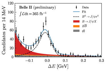
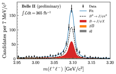
Figure 1: Distributions of (top) $\Delta E$ and (bottom) $m(\ell^{+}\ell^{-})$ for $B^{0}\rightarrow{J\mskip-3.0mu/\mskip-2.0mu\psi\mskip 2.0mu}\pi^{0}$ candidates (data points) with fits overlaid (curves and stacked areas).

From the signal yields, we determine the branching fraction

$${\cal B}=\frac{(n_{\text{sig}}^{e^{+}e^{-}}/{\varepsilon}_{\text{sig}}^{e^{+}e^{-}}+n_{\text{sig}}^{\mu^{+}\mu^{-}}/{\varepsilon}_{\text{sig}}^{\mu^{+}\mu^{-}})(1+f^{+-}/f^{00})}{{\cal B}(J/\psi\rightarrow\ell^{+}\ell^{-}){\cal B}(\pi^{0}\rightarrow\gamma\gamma)2N(B\kern 1.79993pt\overline{\kern-1.79993ptB}{})}$$ (5)

where ${\varepsilon}_{\text{sig}}$ are the efficiencies obtained from simulated signal samples and corrected for differences between data and simulation using control samples, ${\cal B}(J/\psi\rightarrow\ell^{+}\ell^{-})$ is the sum of ${\cal B}(J/\psi\rightarrow e^{+}e^{-})=(5.971\pm 0.032)\%$ and ${\cal B}(J/\psi\rightarrow\mu^{+}\mu^{-})=(5.961\pm 0.033)\%$, ${\cal B}(\pi^{0}\rightarrow\gamma\gamma)$ is $(98.823\pm 0.034)\%$ Navas et al. (2024), $N(B\kern 1.79993pt\overline{\kern-1.79993ptB}{})=(387\pm 6)\times 10^{6}$ is the number of $B\kern 1.79993pt\overline{\kern-1.79993ptB}{}$ pairs in the dataset, and $f^{+-}/f^{00}=1.065\pm 0.052$ is the $B^{+}/B^{0}$ production ratio Choudhury et al. (2023). We obtain ${\cal B}(B^{0}\rightarrow{J\mskip-3.0mu/\mskip-2.0mu\psi\mskip 2.0mu}\pi^{0})=(2.02\pm 0.12)\times 10^{-5}$, where the uncertainty is statistical only. We validate our analysis on the $B^{+}\rightarrow{J\mskip-3.0mu/\mskip-2.0mu\psi\mskip 2.0mu}K^{*+}$ control sample, for which we obtain ${\cal B}(B^{+}\rightarrow{J\mskip-3.0mu/\mskip-2.0mu\psi\mskip 2.0mu}K^{*+})=(1.47\pm 0.04)\times 10^{-3}$, where the uncertainties are statistical only, in agreement with the world average Navas et al. (2024).

Table 1: Signal efficiencies, yields, and purity in the signal region. The signal efficiencies are corrected for differences between data and simulation, and their uncertainties include both statistical and systematic uncertainties, while the uncertainties on the signal yields are statistical only.

Decay mode	${\varepsilon}_{\text{sig}}$ [%]	$n_{\text{sig}}$	Purity [%]
$J/\psi\rightarrow\mu^{+}\mu^{-}$	$48\pm 2$	$204\pm 17$	$80$
$J/\psi\rightarrow e^{+}e^{-}$	$41\pm 2$	$188\pm 17$	$83$

V $C\!P$ asymmetry fit

We determine the $C\!P$ asymmetries from a likelihood fit to the unbinned $\Delta t$ distribution of flavor-tagged candidates in the signal region. Candidates outside of the signal region are removed from the fit as they mostly consist of $B\rightarrow{J\mskip-3.0mu/\mskip-2.0mu\psi\mskip 2.0mu}X$ background events which dilute the observable $C\!P$ asymmetries of the signal. The likelihood function is

$$\begin{split}\mathcal{L}\propto\prod_{i=1}^{N}\bigg{\{}(1-f_{q\overline{}q})\Big{[}(1-f_{B\kern 1.25995pt\overline{\kern-1.25995ptB}{}})\big{(}(1-f_{{J\mskip-3.0mu/\mskip-2.0mu\psi\mskip 2.0mu}X})P_{{J\mskip-3.0mu/\mskip-2.0mu\psi\mskip 2.0mu}\pi^{0}}^{i}\\ +f_{{J\mskip-3.0mu/\mskip-2.0mu\psi\mskip 2.0mu}X}P_{{J\mskip-3.0mu/\mskip-2.0mu\psi\mskip 2.0mu}X}^{i}\big{)}+f_{B\kern 1.25995pt\overline{\kern-1.25995ptB}{}}P_{B\kern 1.25995pt\overline{\kern-1.25995ptB}{}}^{i}\Big{]}+f_{q\overline{}q}P_{q\overline{}q}^{i}\bigg{\}}\end{split}$$ (6)

where $f_{q\overline{}q}$, $f_{B\kern 1.25995pt\overline{\kern-1.25995ptB}{}}$, and $f_{{J\mskip-3.0mu/\mskip-2.0mu\psi\mskip 2.0mu}X}$ are the background fractions in the signal region, determined from the signal extraction fit, and $P^{i}=P(\Delta t^{i})$ is the PDF of the $i$th candidate.

The $\Delta t$ distribution of the signal in Eq. 1 is modified to model the effect of imperfect flavor assignment from the tagging algorithm

$$\begin{split}\mathcal{P}(\Delta t,q)=\frac{e^{-|\Delta t|/\tau_{B^{0}}}}{4\tau_{B^{0}}}\Big{\{}1-q\Delta w+qa^{\rm tag}_{\epsilon}(1-2w)\\ +\big{[}q(1-2w)+a^{\rm tag}_{\epsilon}(1-q\Delta w)\big{]}\\ \times\big{[}S_{C\!P}\sin(\Delta m_{d}\Delta t)-C_{C\!P}\cos(\Delta m_{d}\Delta t)\big{]}\Big{\}},\end{split}$$ (7)

where $w$ is the wrong-tag probability, $\Delta w$ is the wrong-tag probability difference between events tagged as $B^{0}$ and $\kern 1.79993pt\overline{\kern-1.79993ptB}{}^{0}$, and $a^{\rm tag}_{\epsilon}$ is the tagging efficiency asymmetry between $B^{0}$ and $\kern 1.79993pt\overline{\kern-1.79993ptB}{}^{0}$. We divide our sample into intervals of the tag-quality variable $r=1-2w$ provided by the tagging algorithm, to gain statistical sensitivity from events with different wrong-tag fractions. We use the boundaries $(0.0,0.1,0.25,0.45,0.6,0.725,0.875,1.0)$ and corresponding calibration parameters obtained with a sample of $B^{0}\rightarrow D^{*-}\pi^{+}$ decays in Ref. Adachi et al. (2024). The effective flavor tagging efficiency, defined as $\sum_{i}\varepsilon_{i}(1-2w_{i})^{2}$, where $\varepsilon_{i}$ is the fraction of events associated with a tag decision and $w_{i}$ is the wrong-tag probability in the $i$-th $r$-bin, is $(37.40\pm 0.43\pm 0.36)\%$, where the uncertainties are statistical and systematic, respectively Adachi et al. (2024). Since $f_{q\overline{}q}$ varies with $r$, we use the distribution in off-resonance data to scale the average fraction in each bin, while $f_{B\kern 1.25995pt\overline{\kern-1.25995ptB}{}}$ and $f_{B\rightarrow{J\mskip-3.0mu/\mskip-2.0mu\psi\mskip 2.0mu}X}$ are constants in $r$, as verified in simulation.

The effect of finite detector $\Delta t$ resolution is taken into account by modifying Eq. 7 as

$$\mathcal{F}(\Delta t,q|\sigma_{\Delta t})=\int\mathcal{P}(\Delta t^{\prime},q)\mathcal{R}(\Delta t-\Delta t^{\prime}|\sigma_{\Delta t})d\Delta t^{\prime},$$ (8)

where $\mathcal{R}$ is the resolution function, conditional on the per-event $\Delta t$ uncertainty $\sigma_{\Delta t}$. The resolution function is described by the sum of two components:

$$\begin{split}\mathcal{R}(\delta t|&\sigma_{\Delta t})=(1-f_{t}(\sigma_{\Delta t}))G(\delta t|m_{G}\sigma_{\Delta t},s_{G}\sigma_{\Delta t})\\ +&f_{t}(\sigma_{\Delta t})R_{t}(\delta t|m_{t}\sigma_{\Delta t},s_{t}\sigma_{\Delta t},k/\sigma_{\Delta t},f_{>},f_{<})\end{split}$$ (9)

where $\delta t$ is the difference between the observed and the true $\Delta t$. The first component is a Gaussian function with mean $m_{G}$ and width $s_{G}$ scaled by $\sigma_{\Delta t}$, which models the core of the distribution. The second component $R_{t}$ is the sum of a Gaussian function and the convolution of a Gaussian with two oppositely sided exponential functions,

$$\begin{split}R_{t}(x|\mu,\sigma,k,f_{>},f_{<}&)=(1-f_{<}-f_{>})G(x|\mu,\sigma)\\ &+f_{<}G(x|\mu,\sigma)\otimes k\exp_{<}(kx)\\ &+f_{>}G(x|\mu,\sigma)\otimes k\exp_{>}(-kx),\end{split}$$ (10)

where $\exp_{>}(kx)=\exp(kx)$ if $x>0$ or zero otherwise, and similarly for $\exp_{<}(kx)$. The exponential tails arise from intermediate displaced charm-hadron vertices from the $B_{\text{tag}}$ decay. The fraction $f_{t}(\sigma_{\Delta t})$ is zero at low values of $\sigma_{\Delta t}$ and rises steeply to reach a plateau of 0.2 at $\sigma_{\Delta t}=0.25\leavevmode\nobreak\ {\rm\,ps}$. We neglect an outlier component in the resolution, accounting for $\mathcal{O}(10^{-3})$ fraction of events with poorly reconstructed vertices, which shows no impact on the results. We use the same resolution function parameters calibrated with a sample of $B^{0}\rightarrow D^{*-}\pi^{+}$ decays as in Ref. Adachi et al. (2024).

The $B\rightarrow{J\mskip-3.0mu/\mskip-2.0mu\psi\mskip 2.0mu}X$ backgrounds are modeled separately for decays of $B^{0}$ and $B^{+}$ mesons in the $\Delta t$ fit, with effective lifetimes determined from simulation and PDF with the same functional form as the signal. The $C\!P$ asymmetries of the $B^{0}\rightarrow{J\mskip-3.0mu/\mskip-2.0mu\psi\mskip 2.0mu}X$ backgrounds are determined from simulated $B^{0}\rightarrow{J\mskip-3.0mu/\mskip-2.0mu\psi\mskip 2.0mu}K^{0}_{S}$ and $B^{0}\rightarrow{J\mskip-3.0mu/\mskip-2.0mu\psi\mskip 2.0mu}K^{0}_{L}$ decays misreconstructed as signal and the fraction of $B^{+}\rightarrow{J\mskip-3.0mu/\mskip-2.0mu\psi\mskip 2.0mu}X$ backgrounds relative to the total amount of $B\rightarrow{J\mskip-3.0mu/\mskip-2.0mu\psi\mskip 2.0mu}X$ backgrounds is fixed from simulation. The $C\!P$ asymmetries of the $B^{+}\rightarrow{J\mskip-3.0mu/\mskip-2.0mu\psi\mskip 2.0mu}X$ backgrounds are set to zero. The $\Delta t$ distribution of the $B\kern 1.79993pt\overline{\kern-1.79993ptB}{}$ backgrounds is described using an exponential PDF convolved with a Gaussian resolution model determined from simulated data. The distribution of the continuum background is modeled with a double-Gaussian PDF determined from off-resonance data.

We validate the fit by measuring the lifetime on $B^{+}\rightarrow{J\mskip-3.0mu/\mskip-2.0mu\psi\mskip 2.0mu}K^{*+}$ and $B^{0}\rightarrow{J\mskip-3.0mu/\mskip-2.0mu\psi\mskip 2.0mu}K^{0}_{S}$ data. We obtain $\tau_{B^{+}}=(1.559\pm 0.051){\rm\,ps}$ and $\tau_{B^{0}}=(1.513\pm 0.024){\rm\,ps}$, respectively, where the uncertainties are statistical only. We also perform the $C\!P$ asymmetry fit on the $B^{0}\rightarrow{J\mskip-3.0mu/\mskip-2.0mu\psi\mskip 2.0mu}K^{0}_{S}$ sample, for which we obtain $C_{C\!P}=-0.045\pm 0.028$ and $S_{C\!P}=0.688\pm 0.037$, where the uncertainties are statistical only. All the values of the lifetimes and $C\!P$ asymmetries are consistent with the world averages Navas et al. (2024).

The $B^{0}\rightarrow{J\mskip-3.0mu/\mskip-2.0mu\psi\mskip 2.0mu}\pi^{0}$ data are displayed in Fig. 2 with fit projections overlaid. We determine the direct and mixing-induced $C\!P$ asymmetries $C_{C\!P}=0.13\pm 0.12$ and $S_{C\!P}=-0.88\pm 0.17$, where the uncertainties are statistical only. The correlation between $C_{C\!P}$ and $S_{C\!P}$ is $-8\%$. The $\Delta t$ distributions for tagged signal decays, after subtracting the backgrounds Pivk and Le Diberder (2005), are displayed in Fig. 3, along with the decay rate asymmetry.

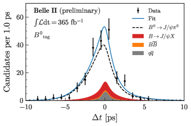
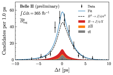
Figure 2: Distributions of $\Delta t$ for (top) $B^{0}$ and (bottom) $\kern 1.79993pt\overline{\kern-1.79993ptB}{}^{0}$-tagged $B^{0}\rightarrow{J\mskip-3.0mu/\mskip-2.0mu\psi\mskip 2.0mu}\pi^{0}$ candidates (data points) with fits overlaid (curves and stacked areas).

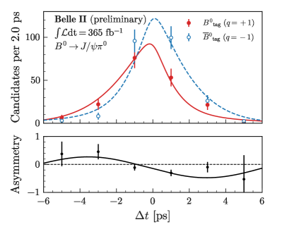
Figure 3: Distributions and fit projections of $\Delta t$ for background-subtracted flavor-tagged $B^{0}\rightarrow{J\mskip-3.0mu/\mskip-2.0mu\psi\mskip 2.0mu}\pi^{0}$ candidates. The fit PDFs corresponding to candidates tagged as $q=-1$ and $q=+$1 are shown as dashed and solid curves, respectively. The decay rate asymmetry, defined as $[N(q=+1)-N(q=-1)]/[N(q=+1)+N(q=-1)]$, is displayed in the bottom subpanel.

VI Systematic Uncertainties

Contributions from all considered sources of systematic uncertainty are listed in Tables 2 and 3 for the branching fraction and $C\!P$ asymmetries, respectively. The leading contribution to the total systematic uncertainty on the branching fraction arises from the $\pi^{0}$ efficiency calibration, while the main systematic uncertainties on the $C\!P$ asymmetries originate from the calibration of the flavor tagging and resolution function with the $B^{0}\rightarrow D^{*-}\pi^{+}$ control sample and tag-side interference.

VI.1 Branching fraction

In the computation of the branching fraction, we correct the signal efficiencies obtained in simulation using control samples from collision data. The statistical and systematic uncertainties associated with the correction factors are propagated to the measurement of the branching fraction systematic uncertainty.

The $\pi^{0}$ reconstruction efficiency is measured in data and simulation using the ratio of the yields of $D^{*+}\rightarrow D^{0}(\rightarrow K^{-}\pi^{+}\pi^{0})\pi^{+}$ and $D^{*+}\rightarrow D^{0}(\rightarrow K^{-}\pi^{+})\pi^{+}$ decays, scaled by the inverse values of their branching fractions. The yield ratio in experimental and simulated data is used to obtain correction factors as functions of the $\pi^{0}$ polar angle and momentum. The average correction factor over the kinematic distribution of the $\pi^{0}$ in $B^{0}\rightarrow{J\mskip-3.0mu/\mskip-2.0mu\psi\mskip 2.0mu}\pi^{0}$ decays is $1.05\pm 0.04$, where the uncertainty is dominated by the knowledge of the $D^{0}$ branching fractions Navas et al. (2024).

The difference in electron and muon identification performance between simulation and experimental data is calibrated using ${J\mskip-3.0mu/\mskip-2.0mu\psi\mskip 2.0mu}\rightarrow\ell^{+}\ell^{-}$, $e^{+}e^{-}\rightarrow\ell^{+}\ell^{-}(\gamma)$ and $e^{+}e^{-}\rightarrow e^{+}e^{-}\ell^{+}\ell^{-}$ samples. The average correction factor over the kinematic distribution of the signal is $1.002\pm 0.006$ for the $J/\psi\rightarrow e^{+}e^{-}$ mode and $0.938\pm 0.005$ for the $J/\psi\rightarrow\mu^{+}\mu^{-}$ mode, where the uncertainties are the sum in quadrature of the statistical and systematic uncertainties.

The performance of the continuum-suppression BDT is validated using the $B^{0}\rightarrow{J\mskip-3.0mu/\mskip-2.0mu\psi\mskip 2.0mu}K^{0}_{S}$ control sample. The ratio of the signal efficiency after applying the BDT requirement in data and simulation is found to be $1.001\pm 0.004$ and $1.007\pm 0.003$ for the $J/\psi\rightarrow e^{+}e^{-}$ and $J/\psi\rightarrow\mu^{+}\mu^{-}$ modes, respectively, where the uncertainties are statistical only.

Tracking efficiencies are measured using $e^{+}e^{-}\rightarrow\tau^{+}\tau^{-}$ events, where one $\tau$ decays as $\tau^{-}\rightarrow e^{-}\overline{\nu}_{e}\nu_{\tau}$ and the other as $\tau^{-}\rightarrow\pi^{-}\pi^{+}\pi^{-}\nu_{\tau}$. Efficiencies for data and simulation are found to be compatible within an uncertainty of $0.27\%$, which is propagated for each track to the uncertainty on the branching fraction.

Table 2: Relative systematic uncertainties on the branching fraction compared with the statistical uncertainties.

Source	Relative uncertainty on BF$[\%]$
$\pi^{0}$ efficiency	$3.7$
Lepton ID	$0.4$
BDT	$0.3$
Tracking efficiencies	$0.5$
External inputs	$0.4$
$N(B\kern 1.79993pt\overline{\kern-1.79993ptB}{})$	$1.4$
$f^{+-}/f^{00}$	$2.5$
Fixed parameters	$0.9$
Backgrounds composition	$0.4$
Multiple candidates	$0.5$
Total systematic uncertainty	$4.9$
Statistical uncertainty	$6.0$

We propagate the uncertainty on the branching fractions of the ${J\mskip-3.0mu/\mskip-2.0mu\psi\mskip 2.0mu}$ and $\pi^{0}$ decay modes used to reconstruct the signal Navas et al. (2024). The uncertainty on the number of $B^{0}$ mesons in the sample arises from the measurement of the number of $B\kern 1.79993pt\overline{\kern-1.79993ptB}{}$ pairs and from the knowledge of the $B^{+}/B^{0}$ production ratio Choudhury et al. (2023). Both uncertainties are propagated to the branching fraction and included in the systematic uncertainty.

We consider the uncertainties associated with the determination of the signal yields from the fit in the following way. We repeat the fit by fixing the parameters determined in the control samples to alternative values chosen according to their statistical covariance matrix. We take the standard deviation of the distribution of the signal yields thus obtained and propagate it to the branching fraction. To account for differences in the composition of the backgrounds between data and simulation, we use simplified simulated datasets where each component is generated according to their PDFs. The main $B\rightarrow{J\mskip-3.0mu/\mskip-2.0mu\psi\mskip 2.0mu}X$ background components are generated with independent $\Delta E$ distributions and their yields varied between $\pm 20\%$ and $\pm 50\%$ from the expected value. We fit these datasets using the nominal fit model and obtain an average bias on the signal yields for each alternative background configuration. We verify that these variations in the background yields cover possible disagreements between data and simulation by comparing their distributions with sidebands enriched in different type of backgrounds. We define a sideband with $M_{\rm bc}^{\prime}<5.27\leavevmode\nobreak\ {\mathrm{\,Ge\kern-1.00006ptV\!/}c^{2}}$ and $m(\gamma\gamma)\in[0.1,0.16]\leavevmode\nobreak\ {\mathrm{\,Ge\kern-1.00006ptV\!/}c^{2}}$, where the backgrounds with properly reconstructed $\pi^{0}$ candidates are dominant, and a sideband with $M_{\rm bc}^{\prime}>5.27\leavevmode\nobreak\ {\mathrm{\,Ge\kern-1.00006ptV\!/}c^{2}}$ and $m(\gamma\gamma)\in[0.02,0.1]\cup[0.16,0.2]\leavevmode\nobreak\ {\mathrm{\,Ge\kern-1.00006ptV\!/}c^{2}}$, where the backgrounds with mis-reconstructed $\pi^{0}$ candidates are dominant. We also account for variations in the $B\kern 1.79993pt\overline{\kern-1.79993ptB}{}$ background yield and fraction of signal with a misreconstructed $\pi^{0}$ using the same approach. We take the standard deviation of the distribution of the biases as a systematic uncertainty and propagate it to the branching fraction.

Finally, we repeat our measurement on ensembles of simulated data using alternative candidate selection requirements for events with multiple candidates. For each selection, we obtain an average bias on the signal yields. We take the standard deviation of the distribution of the average biases as a systematic uncertainty and propagate it to the branching fraction.

VI.2 $C\!P$ asymmetries

We consider the uncertainties associated with the flavor tagging and resolution function calibration. We repeat the $C\!P$ asymmetry fit by fixing the calibration parameters determined in the $B^{0}\rightarrow D^{*-}\pi^{+}$ sample to alternative values chosen according to their statistical covariance matrix Adachi et al. (2024). We also repeat the fit by varying the same set of parameters within their systematic uncertainties without correlations. In both cases, we take as a systematic uncertainty the standard deviation of the $C\!P$ asymmetries distribution thus obtained, and sum them in quadrature.

We propagate the statistical uncertainties on the signal and background fractions to the $C\!P$ asymmetries. We repeat the $C\!P$ asymmetry fit by fixing the yields and continuum background fractions determined in the signal extraction fit to alternative values chosen according to their statistical covariance matrix. The standard deviation of the distribution of the $C\!P$ asymmetries thus obtained is assigned as a systematic uncertainty.

Table 3: Systematic uncertainties on the $C\!P$ asymmetries compared with the statistical uncertainties.

Source	$C_{C\!P}$	$-\eta_{f}S_{C\!P}$
Calibration with $B^{0}\rightarrow D^{*-}\pi^{+}$	$0.017$	$0.023$
Signal extraction fit	$0.003$	$0.017$
Backgrounds composition	$0.005$	$0.009$
Backgrounds $\Delta t$ shapes	$<0.001$	$0.001$
Fit bias	$0.010$	$0.010$
Multiple candidates	$<0.001$	$0.002$
Tracking detector misalignment	$0.002$	$0.002$
Tag-side interference	$0.027$	$0.001$
$\tau_{B^{0}}$ and $\Delta m_{d}$	$<0.001$	$<0.001$
Total systematic uncertainty	$0.034$	$0.032$
Statistical uncertainty	$0.123$	$0.171$

In order to estimate the systematic uncertainty associated with the background model, we use the ensembles generated with alternative background compositions used for the study of the systematic uncertainties on the branching fraction. These simplified simulated datasets are also generated with different $\Delta t$ distributions for the main $B\rightarrow{J\mskip-3.0mu/\mskip-2.0mu\psi\mskip 2.0mu}X$ background components. In particular, the $B^{0}\rightarrow{J\mskip-3.0mu/\mskip-2.0mu\psi\mskip 2.0mu}K^{0}_{S}$ and $B^{0}\rightarrow{J\mskip-3.0mu/\mskip-2.0mu\psi\mskip 2.0mu}K^{0}_{L}$ backgrounds are generated using the known value of their $C\!P$ asymmetries Navas et al. (2024). We generate separately an additional prompt component in $\Delta t$ originating from tracks of the signal-side that are included in the fit of the tag-side vertex. We fit these datasets using the nominal fit model and obtain an average bias on the $C\!P$ asymmetries for each alternative background configuration. We take the standard deviation of the distribution of these biases as a systematic uncertainty.

We also consider the variations of the parameters of the $\Delta t$ PDF of the continuum background using the covariance matrix determined in the fit to the off-resonance data. We take as systematic uncertainty the standard deviation of the distribution of the $C\!P$ asymmetries thus obtained.

We estimate a fit bias, due to the combined effects of the approximate determination of $\Delta t$ in Eq. 3 and differences between the signal and calibration sample, using simulated signal events generated with $C_{C\!P}$ in $[-0.4,0.4]$ and $S_{C\!P}$ in $[-1.0,0.0]$ in steps of $0.2$. In the nominal fit to the data, we correct the $C\!P$ asymmetries for their bias ($0.010\pm 0.001$ on $C_{C\!P}$ and $-0.011\pm 0.001$ on $S_{C\!P}$, where the uncertainties come from the size of the simulated sample) and assign the absolute value of the bias (0.01) as a systematic uncertainty.

The same procedure used to estimate the impact of the candidate selection on the measurement of the branching fraction is repeated for the $C\!P$ asymmetries.

We study the impact of the tracking detector misalignment on the $C\!P$ asymmetries using simulated samples reconstructed with various misalignment configurations and assign as a systematic uncertainty the sum in quadrature of the differences with respect to the nominal alignment configuration.

We estimate the shift from the true values of the $C\!P$ asymmetries due to the tag-side interference, i.e., neglecting the effect of CKM-suppressed $b\rightarrow u\overline{}cd$ decays in the $B_{\text{tag}}$ in the model for $\Delta t$, using the estimators for $C_{C\!P}$ and $S_{C\!P}$ that reproduce this bias as given in Ref. Long et al. (2003). Since the sign of the bias depends on the strong phase difference between the favored and suppressed decays, which is poorly known, we take the maximum absolute value as a systematic uncertainty.

The values of the $B^{0}$ lifetime and oscillation frequency are fixed in the PDF. To estimate the corresponding systematic uncertainties, we vary them around their known values according to their uncertainties Navas et al. (2024). We find that this has negligible impact on the $C\!P$ asymmetries.

VII Summary

We report a measurement of the branching fraction and $C\!P$ asymmetries in $B^{0}\rightarrow{J\mskip-3.0mu/\mskip-2.0mu\psi\mskip 2.0mu}\pi^{0}$ decays using data from the Belle II experiment. We find $392\pm 24$ signal decays in a sample containing $(387\pm 6)\times 10^{6}$ $B\kern 1.79993pt\overline{\kern-1.79993ptB}{}$ events, corresponding to a value of the branching fraction of

$$\mathcal{B}(B^{0}\rightarrow{J\mskip-3.0mu/\mskip-2.0mu\psi\mskip 2.0mu}\pi^{0})=(2.02\pm 0.12\pm 0.10)\times 10^{-5},$$ (11)

where the first uncertainty is statistical, and the second is systematic. The result is consistent with the world average Navas et al. (2024) and has comparable precision to previous determinations.

We obtain the following values of the $C\!P$ asymmetries

$$\begin{split}C_{C\!P}&=0.13\pm 0.12\pm 0.03,\\ S_{C\!P}&=-0.88\pm 0.17\pm 0.03,\end{split}$$ (12)

where the first uncertainty is statistical, and the second is systematic. The results are the most precise to date and are consistent with previous determinations from Belle and BABAR Aubert et al. (2008); Pal et al. (2018). The central value of $S_{C\!P}$ is $5.0$ standard deviations from zero. The significance is calculated using the sum in quadrature of the statistical and systematic uncertainties. This is the first observation of mixing-induced $C\!P$ violation in $B^{0}\rightarrow{J\mskip-3.0mu/\mskip-2.0mu\psi\mskip 2.0mu}\pi^{0}$ decays from a single measurement. The improved determinations of the branching fraction and $C\!P$ asymmetries in this mode provide further constraints on the penguin parameters and on the extraction of the CKM angle $\phi_{1}$ Barel et al. (2021).

References

- Cabibbo (1963) N. Cabibbo, Phys. Rev. Lett. 10, 531 (1963).
- Kobayashi and Maskawa (1973) M. Kobayashi and T. Maskawa, Prog. Theor. Phys. 49, 652 (1973).
- Aubert et al. (2009) B. Aubert et al. (BABAR Collaboration), Phys. Rev. D 79, 072009 (2009).
- Adachi et al. (2012) I. Adachi et al. (Belle Collaboration), Phys. Rev. Lett. 108, 171802 (2012).
- Aaij et al. (2024a) R. Aaij et al. (LHCb Collaboration), Phys. Rev. Lett. 132, 021801 (2024a).
- Grossman and Worah (1997) Y. Grossman and M. P. Worah, Physics Letters B 395, 241 (1997).
- Amhis et al. (2023) Y. S. Amhis et al. (HFLAV Collaboration), Phys. Rev. D 107, 052008 (2023).
- Charles et al. (2005) J. Charles et al. (CKMfitter Group), Eur. Phys. J. C 41, 1 (2005), updated results and plots available at: http://ckmfitter.in2p3.fr.
- Bona et al. (2005) M. Bona et al. (UTfit Collaboration), JHEP 07, 028 (2005), see also online updates at http://www.utfit.org.
- Ciuchini et al. (2005) M. Ciuchini, M. Pierini, and L. Silvestrini, Phys. Rev. Lett. 95, 221804 (2005).
- Barel et al. (2021) M. Z. Barel, K. D. Bruyn, R. Fleischer, and E. Malami, Journal of Physics G: Nuclear and Particle Physics 48, 065002 (2021).
- Barel et al. (2023) M. Barel, K. De Bruyn, R. Fleischer, and E. Malami, PoS CKM2021, 111 (2023).
- Aubert et al. (2008) B. Aubert et al. (BABAR Collaboration), Phys. Rev. Lett. 101, 021801 (2008).
- Pal et al. (2018) B. Pal et al. (Belle Collaboration), Phys. Rev. D 98, 112008 (2018).
- Avery et al. (2000) P. Avery et al. (CLEO Collaboration), Phys. Rev. D 62, 051101 (2000).
- Navas et al. (2024) S. Navas et al. (Particle Data Group Collaboration), Phys. Rev. D 110, 030001 (2024).
- Aaij et al. (2024b) R. Aaij et al. (LHCb Collaboration), JHEP 05, 065 (2024b).
- Akai et al. (2018) K. Akai, K. Furukawa, and H. Koiso, Nucl. Instrum. Meth. A907, 188 (2018).
- (19) T. Abe et al. (Belle II Collaboration), arXiv:1011.0352 .
- (20) I. Adachi et al. (Belle II Collaboration), arXiv:2407.00965 .
- Adachi et al. (2024) I. Adachi et al. (Belle II Collaboration), Phys. Rev. D 110, 012001 (2024).
- Adamczyk et al. (2022) K. Adamczyk et al. (Belle II SVD Collaboration), J. Instrum. 17, P11042 (2022).
- Jadach et al. (2000) S. Jadach, B. F. L. Ward, and Z. Wa̧s, Comput. Phys. Commun. 130, 260 (2000).
- Sjöstrand et al. (2015) T. Sjöstrand et al., Comput. Phys. Commun. 191, 159 (2015).
- Lange (2001) D. J. Lange, Nucl. Instrum. Methods Phys. Res., Sect A 462, 152 (2001).
- Agostinelli et al. (2003) S. Agostinelli et al. (GEANT4 Collaboration), Nucl. Instrum. Methods Phys. Res., Sect. A 506, 250 (2003).
- Lewis et al. (2019) P. M. Lewis et al., Nucl. Instrum. Meth. A 914, 69 (2019).
- Liptak et al. (2022) Z. J. Liptak et al., Nucl. Instrum. Meth. A 1040, 167168 (2022).
- Kuhr et al. (2019) T. Kuhr, C. Pulvermacher, M. Ritter, T. Hauth, and N. Braun (Belle II Framework Software Group), Comput. Software Big Sci. 3, 1 (2019).
- (30) https://doi.org/10.5281/zenodo.5574115.
- Bertacchi et al. (2021) V. Bertacchi et al. (Belle II Tracking Group), Comput. Phys. Commun. 259, 107610 (2021).
- Milesi et al. (2020) M. Milesi, J. Tan, and P. Urquijo, EPJ Web Conf. 245, 06023 (2020).
- Hulsbergen (2005) W. D. Hulsbergen, Nucl. Instrum. Methods 552, 566 (2005).
- Krohn et al. (2020) J.-F. Krohn et al. (Belle II Analysis Software Group), Nucl. Instrum. Methods Phys. Res., Sect. A 976, 164269 (2020).
- Waltenberger et al. (2008) W. Waltenberger, W. Mitaroff, F. Moser, B. Pflugfelder, and H. V. Riedel, J. Phys. Conf. Ser. 119, 032037 (2008).
- Dey and Soffer (2020) S. Dey and A. Soffer, Springer Proc. Phys. 248, 411 (2020).
- Ed. A. J. Bevan, B. Golob, Th. Mannel, S. Prell, and B. D. Yabsley (2014) Ed. A. J. Bevan, B. Golob, Th. Mannel, S. Prell, and B. D. Yabsley, Eur. Phys. J. C74, 3026 (2014), see Section 6.5.2.
- Fox and Wolfram (1978) G. C. Fox and S. Wolfram, Phys. Rev. Lett. 41, 1581 (1978).
- Chen and Guestrin (2016) T. Chen and C. Guestrin, Proceedings of the 22nd ACM SIGKDD International Conference on Knowledge Discovery and Data Mining, (Association for Computing Machinery, New York, USA, 2016).
- Asner et al. (1996) D. M. Asner et al., Phys. Rev. D 53, 1039 (1996).
- Lee et al. (2003) S. H. Lee et al. (Belle Collaboration), Phys. Rev. Lett. 91, 261801 (2003).
- Bjorken and Brodsky (1970) J. D. Bjorken and S. J. Brodsky, Phys. Rev. D 1, 1416 (1970).
- Brandt et al. (1964) S. Brandt, C. Peyrou, R. Sosnowski, and A. Wroblewski, Phys. Lett. 12, 57 (1964).
- Farhi (1977) E. Farhi, Phys. Rev. Lett. 39, 1587 (1977).
- Cheema (2024) P. Cheema, EPJ Web of Conf. 295, 09035 (2024).
- Gaiser (1982) J. Gaiser, Ph.D. thesis, Stanford University (1982).
- Skwarnicki (1986) T. Skwarnicki, Ph.D. thesis, Cracow, INP (1986).
- Choudhury et al. (2023) S. Choudhury et al. (Belle Collaboration), Phys. Rev. D 107, L031102 (2023).
- Pivk and Le Diberder (2005) M. Pivk and F. R. Le Diberder, Nucl. Instrum. Methods Phys. Res., Sect. A 555, 356 (2005).
- Long et al. (2003) O. Long, M. Baak, R. N. Cahn, and D. Kirkby, Phys. Rev. D 68, 034010 (2003).