The NuSTAR Local AGN $N_{\rm H}$ Distribution Survey (NuLANDS) I: Towards a Truly Representative Column Density Distribution in the Local Universe

Abstract

Hard X-ray-selected samples of Active Galactic Nuclei (AGN) provide one of the cleanest views of supermassive black hole accretion, but are biased against objects obscured by Compton-thick gas column densities of $N_{\rm H}$ $>$ 10²⁴ cm^-2. To tackle this issue, we present the NuSTAR Local AGN $N_{\rm H}$ Distribution Survey (NuLANDS)—a legacy sample of 122 nearby ($z$ $<$ 0.044) AGN primarily selected to have warm infrared colors from IRAS between 25 – 60 $\mu$m. We show that optically classified type 1 and 2 AGN in NuLANDS are indistinguishable in terms of optical [O iii] line flux and mid-to-far infrared AGN continuum bolometric indicators, as expected from an isotropically selected AGN sample, while type 2 AGN are deficient in terms of their observed hard X-ray flux. By testing many X-ray spectroscopic models, we show the measured line-of-sight column density varies on average by $\sim$ 1.4 orders of magnitude depending on the obscurer geometry. To circumvent such issues we propagate the uncertainties per source into the parent column density distribution, finding a directly measured Compton-thick fraction of 35 $\pm$ 9%. By construction, our sample will miss sources affected by severe narrow-line reddening, and thus segregates sources dominated by small-scale nuclear obscuration from large-scale host-galaxy obscuration. This bias implies an even higher intrinsic obscured AGN fraction may be possible, although tests for additional biases arising from our infrared selection find no strong effects on the measured column-density distribution. NuLANDS thus holds potential as an optimized sample for future follow-up with current and next-generation instruments aiming to study the local AGN population in an isotropic manner.

citnum

1 Introduction

1.1 AGN Growth and Obscuration

The integrated X-ray emission from accreting supermassive black holes (log $M_{\rm BH}\,/\,M_{\odot}$ $\sim$ 6 – 9.5), or Active Galactic Nuclei (AGN), across cosmic time dominates the Cosmic X-ray Background spectrum (CXB; Giacconi et al. 1962) across the wide energy range E $\sim$ 1 – 300 keV (e.g., Setti & Woltjer 1989; Comastri et al. 1995; Mushotzky et al. 2000; Gandhi & Fabian 2003; Gilli et al. 2007; Treister et al. 2009; Ueda et al. 2014; Brandt & Alexander 2015; Ramos Almeida & Ricci 2017; Ananna et al. 2019, 2020; Civano et al. 2024). Hence, the evolution of and accretion onto supermassive black holes is preserved in the broadband CXB. In particular, AGN in the Seyfert luminosity range ($L_{2-10\,{\rm keV}}$ $\sim$ 10⁴² – 10⁴⁴ erg s^-1) completely dominate the CXB emissivity to beyond $z$ = 1, and contribute between $\approx$ 30 – 50% of the emissivity between $z$ = 1 – 5 (Ueda et al., 2014; Buchner et al., 2015; Aird et al., 2015). These sources are thus crucial to understand, but are best probed in detail in the local universe where fluxes are brighter overall and off-nuclear contaminants can be resolved in the lowest luminosity sources.

Disentangling the evolution and growth of AGN responsible for the observed CXB spectrum (known as population synthesis) requires knowledge of the obscuring neutral hydrogen column density ($N_{\mathrm{H}}$) distribution, which is predicted to co-evolve with accreting supermassive black holes (e.g., Ueda et al. 2014; Buchner et al. 2015; Brandt & Alexander 2015; Hickox & Alexander 2018; Brandt & Yang 2022). This is particularly important because the majority of AGN are known to be obscured, typically defined as having $N_{\mathrm{H}}$  $\gtrsim 10^{22}$ cm^-2 (Risaliti et al., 1999; Burlon et al., 2011; Ricci et al., 2015; Koss et al., 2017). Absorption can occur over a broad range of host-galaxy spatial scales, but the $\sim$ parsec-scale obscuring torus of AGN unification schemes plays a key role in AGN detectability and classification (e.g., Antonucci 1993; Urry & Padovani 1995; Alexander & Hickox 2012; Brandt & Alexander 2015; Netzer 2015; Ramos Almeida & Ricci 2017; Alonso-Tetilla et al. 2024). Hard X-ray ($E>$ 10 keV) photons rarely interact with obscuring gas of $N_{\mathrm{H}}$  $\lesssim 10^{23.5}$ cm^-2 (see e.g., Figure 1 of Boorman et al. 2018). Hard X-ray observations are thus a very effective means of sampling AGN populations, unbiased by mild obscuration ($N_{\mathrm{H}}$  $\lesssim 10^{24}$ cm^-2; e.g., the BeppoSAX High-Energy Large Area Survey: Fiore et al. 1998, the INTEGRAL AGN sample: Malizia et al. 2009, the Swift/BAT Surveys: Ricci et al. 2017a, the NuSTAR Serendipitous Surveys: Lansbury et al. 2017; Greenwell et al. 2024b).

Figure 1: For a given line-of-sight column density, each panel shows the fraction of detected hard 14 – 195 keV flux relative to the escaping flux at the minimum column density allowed by each model ($N_{\rm H,\,0}$). The top right of each panel shows a cartoon for the geometry assumed in each model. For visual clarity, the approximate column density corresponding to 50% depletion is shown with dashed lines for each model, showing a substantial drop in detected hard X-ray flux at high column densities ($N_{\rm H}$ $\gtrsim$ $10^{24.5}$ cm^-2). We additionally show the spread in predicted depletion factors relative to an additional parameter per model. From the upper left to lower left panels in a clockwise direction, the models are: BNsphere (Brightman & Nandra, 2011a), coupled MYtorus (Murphy & Yaqoob, 2009); coupled borus02 (Baloković et al., 2018); warped-disk (Buchner et al., 2021); UXCLUMPY (Buchner et al., 2019); XCLUMPY (Tanimoto et al., 2018). Note for warped-disk, the disk fraction corresponds to the warp extent where 0 and 1 represent flat and strong warp geometries, respectively. To reproduce $N_{\rm H}$ $<$ $10^{24}$ cm^-2 fluxes accurately with warped-disk, we freeze NHLOS to 0.01, and include an optically-thin absorber separately – see the warped-disk documentation for more information.

For column densities in excess of the inverse Thomson cross-section ($N_{\mathrm{H}}$  $\sim 1.5\times 10^{24}$ cm^-2), gas becomes optically thick to Compton scattering and is referred to as Compton-thick. The directly transmitted component of X-ray flux is diminished via photo-electric absorption $\lesssim$ 10 keV with Compton scattering dominating above $\gtrsim$ 10 keV (Lightman & White 1988; Reynolds 1999). At $N_{\mathrm{H}}$ $\gg 10^{25}$ cm^-2 the transmitted/unabsorbed fraction of hard X-ray photons through the obscuration is negligible relative to the Compton-scattered photons (see Figure 1). Instead, the observed flux is almost entirely due to scattering of photons off the optically-thick surface of circumnuclear material directed into the line-of-sight. These ‘reprocessing-dominated’ Compton-thick AGN are the most difficult population to detect in X-ray surveys (e.g., Matt et al. 2000; Comastri et al. 2015; Padovani et al. 2017), and even in the very local universe, X-ray flux-limited surveys are biased against Compton-thick AGN detection (e.g., Figure 3 of Ricci et al. 2015, Koss et al. 2016, Annuar et al., in prep.). Compounding these detection/selection biases is the issue of source characterization/classification (see Section 3). Additional confusion can arise from comparatively strong reprocessed components from the intrinsic accretion disk vs. typical torus geometries (e.g., Gandhi et al. 2007; Treister et al. 2009; Vasudevan et al. 2016; Avirett-Mackenzie & Ballantyne 2019). Conversely, heavily obscured AGN signatures may be swamped by other spectral components resulting in erroneous low-column estimates in the case of low signal-to-noise or band-limited X-ray data (as demonstrated in e.g., Civano et al. 2015; Gandhi et al. 2017; Boorman et al. 2018).

The result is that the fraction of Compton-thick AGN remains uncertain, and hotly debated. X-ray surveys of the local universe typically find an observed Compton-thick fraction of $\lesssim 15$% (e.g., Masini et al. 2018; Georgantopoulos & Akylas 2019; Torres-Albà et al. 2021), and is increased to intrinsic fractions of $\sim$10 – 30% after applying X-ray-specific bias corrections (e.g., Burlon et al. 2011; Ricci et al. 2015; Koss et al. 2016). But higher Compton-thick fractions are often discussed in the literature; for example, Ananna et al. (2019) require 50 $\pm$ 9% of all AGN within $z$ $\sim$ 0.1 to be Compton-thick based on observed survey flux distributions and the CXB. The local $N_{\mathrm{H}}$ distribution is the $z$ = 0 boundary condition imposed in CXB synthesis models (e.g., Ueda et al. 2014), so accurate determination of the number of obscured and Compton-thick AGN locally is crucial. Independent selection strategies are required at different wavelengths that are not biased against detection of highly obscured AGN in the same way as X-ray flux-limited surveys.

1.2 Representative AGN Selection

Complementary methodologies for isotropic AGN selection include (i) optical narrow-line emission, (ii) radio low-frequency surveys, (iii) mid-infrared narrow-line emission, and (iv) mid-to-far infrared continuum emission (e.g., reviewed in Hickox & Alexander 2018). These techniques are effective because the unified scheme of AGN ascribes observed differences between AGN classes primarily to the orientation of the torus relative to the line-of-sight, whereas all the above methods probe AGN emission on much larger scales.

1. Optical narrow-line emission: Originating in the narrow-line region, optical emission lines have been successfully used to select ‘optimally’ matched samples of X-ray obscured and unobscured sources (e.g., Risaliti et al. 1999; Kammoun et al. 2020), by treating forbidden transitions such as the [Oiii] $\lambda$ 5007 Å emission line as ‘bolometric’ estimators of AGN power. The $\sim$ kpc-scale extension of the narrow-line region means its emission should be relatively insensitive to $\sim$ pc-scale torus orientation angles. While certainly an effective means of identifying AGN that are heavily obscured in X-rays, this technique requires intensive spectroscopic surveys of large sky areas. In addition, geometric variations, time variability and dust content can cause significant inherent scatter in the [O iii] power, implying that it is not a strict and accurate estimator of the current bolometric AGN power (e.g., Saunders et al. 1989; Boroson & Green 1992; Netzer & Laor 1993; Zakamska et al. 2003; Berney et al. 2015; Ueda et al. 2015; Finlez et al. 2022). Additional complications would arise from selecting AGN encompassed by very high – or even 4$\pi$ – covering factors of obscuration and/or significant host galaxy obscuration, as the narrow-line region would not be illuminated at all (see discussion in Boroson & Green 1992; Goulding & Alexander 2009; Koss et al. 2010; Greenwell et al. 2024a for more information).

2. Radio/mm interferometric surveys: Radio continuum luminosity can serve as an isotropic indicator of the time-averaged intrinsic AGN power (e.g., Wilkes et al. 2013; Kuraszkiewicz et al. 2021). This is true for the unbeamed extended jet component, which is best probed at low frequencies (e.g., Orr & Browne 1982; Giuricin et al. 1990; Singh et al. 2013; Gürkan et al. 2019), and increasing evidence suggests that radio jets are likely a common component of radiatively efficient accretion (e.g., Jarvis et al. 2019). However, the majority of radio surveys to date have only been able to resolve large-scale jets, which so far have been found to be uncommon in radiatively efficient AGN (e.g., Panessa et al. 2016). This means the source yield per unit volume with such surveys is currently typically small. However, ongoing surveys (with e.g., the LOw-Frequency ARray; LOFAR, Australian Square Kilometre Array Pathfinder; ASKAP, Meer Karoo Array Telescope; MeerKAT) as well as future surveys (with e.g., the Square Kilometer Array; SKA) will find ever-increasing numbers of radiatively efficient AGN with lower-power/small-scale jets, enabling the selection of statistically large samples of such AGN directly in the radio (Jarvis, 2007; Baldi et al., 2018; Hardcastle et al., 2019; Sabater et al., 2019; Hardcastle & Croston, 2020; Williams et al., 2022; Igo et al., 2024; Mazzolari et al., 2024). At low radio power, the observed radio emission may originate from non-jet sources (Panessa et al., 2019) and such future surveys will thus help to shed light on the large intrinsic scatter around the correlation between jet power and AGN luminosity (Hickox et al. 2014; Mingo et al. 2016), ultimately allowing improved determination of intrinsic AGN power from radio observations. Promising developments have also been made recently with high-frequency ($>$ 10 GHz) radio emission, with indications that with sufficient sensitivity the compact corona-powered radio emission can be almost universally detected for both radio-loud and radio-quiet AGN even at extremely high line-of-sight column densities (e.g., $N_{\rm H}$ $\sim$ 10²⁷ cm^-2; Smith et al. 2020; Kawamuro et al. 2022; Ricci et al. 2023, Magno et al., in prep.).

3. Mid-infrared line emission: Complementary to optical lines, narrow-line emission can also be excited in the infrared by AGN activity. Commonly used lines include the [Nev] $\lambda$ 14/24 $\mu$m and [Oiv] $\lambda$ 26 $\mu$m emission lines, both of which have been adopted for isotropic AGN selection and tests of unification (e.g., Goulding & Alexander 2009; Gilli et al. 2010; Dicken et al. 2014; Yang et al. 2015). Their high ionization potentials imply that they are better than the optical lines at disentangling AGN activity from star-formation. Additionally, their low optical depths allow probing through high extinction levels from both the host galaxy and nuclear regions. However, intensive infrared spectroscopic surveys are even more sparse than in the optical, and these lines are subject to substantial scatter (e.g., Meléndez et al. 2008; Rigby et al. 2009; Diamond-Stanic et al. 2009; LaMassa et al. 2010; Asmus 2019; Cleri et al. 2023; Barchiesi et al. 2024). Also even though the line fluxes are expected to be relatively immune to high column densities, the photo-ionising photons required to excite the lines can be obscured in high covering factor scenarios. Ongoing work with the James Webb Space Telescope (JWST; Gardner et al. 2023) Mid-Infrared Instrument (MIRI; Rieke et al. 2015; Wells et al. 2015; Wright et al. 2015) holds strong potential for probing the physical origin of various mid-infrared spectral features in nearby Seyfert AGN (e.g., García-Bernete et al. 2024; Davies et al. 2024; Hermosa Muñoz et al. 2024; Haidar et al. 2024).

4. Mid-to-far infrared continuum: Infrared AGN continuum emission partly arises from dust-reprocessing in the torus, and is thus associated with much larger size scales than the $\sim$ 10^-5 – 10^-4 pc-scale X-ray emitting corona. In addition, a significant infrared component sometimes arises on even larger scales from ‘polar’ dust in the inner narrow-line region (Hönig et al., 2013; Asmus et al., 2016; Fuller et al., 2019; Asmus, 2019). A combination of low absorption optical depth in the infrared, together with the extended physical scales results in the emission appearing largely isotropic of AGN optical type (e.g., Buchanan et al. 2006; Levenson et al. 2009; Hönig et al. 2011). This has been shown to be the case for optically classified type 1 and 2 AGN, including X-ray classified heavily obscured and Compton-thick AGN (e.g., Gandhi et al. 2009; Asmus et al. 2015). Longer (mid-to-far infrared) wavelengths appear to be more isotropic than the near-infrared (e.g., Hönig et al. 2011; Mateos et al. 2015). Deviations from isotropy are mild in the mid-infrared, estimated to be a factor of $\lesssim$ 1.4 at 12 $\mu$m, relative to the intrinsic 2 – 10 keV X-ray emission (Asmus et al., 2015). The scatter of the correlation between the infrared and X-ray powers is also relatively small, at $\approx$ 0.35 dex (e.g., Asmus et al. 2015). This is clearly a complex region with emission occurring over multiple nuclear scales, and there is much debate regarding its nature. For our purposes discussed below, the important factor is the emission isotropy from different AGN obscuration classifications, and we expand our definition of the torus to include the entire nuclear structure including the classical toroidal obscurer and any polar component. Whilst an almost isotropic selector of AGN type (e.g., Alexander 2001), aperture-dependent infrared continuum selection is not 100% reliable, and contaminating host-galaxy emission in particular needs to be considered (e.g., Lacy et al. 2007; Stern et al. 2012; Mateos et al. 2012; Assef et al. 2018; Hickox & Alexander 2018; Asmus et al. 2020).

While each of the above techniques provides a means of isotropic AGN selection to first order, each has associated advantages and disadvantages. So how should one quantify the effectiveness of any one strategy relative to another? This is best done by comparing sample properties according to multiple bolometric power indicators, which requires the construction of samples with several of the above indicators.

We aim to devise a survey strategy in a way that is more representative of the underlying range of AGN obscuration than X-ray flux-limited selection (see Figure 1), especially in the extreme $N_{\mathrm{H}}$ regime. This work adopts infrared continuum selection. We are guided to this choice because (i) of the availability of legacy all-sky infrared imaging surveys, which (ii) allow collation of substantial AGN sample sizes with (iii) follow-up optical source classification already available. In this way, we can compare sample properties in the parameter space of infrared continuum, optical emission line, and hard X-ray bolometric indicators. Finally, we require high-quality broadband X-ray spectral characterization for $N_{\mathrm{H}}$ measurement.

Our survey is the NuSTAR Local AGN $N_{\rm H}$ Distribution Survey (NuLANDS), and is a continuation of the Warm IRAS Sample (de Grijp et al., 1985, 1987). The sample derivation follows in Section 2, with Section 3 presenting updated optical classifications to highlight its AGN type isotropy. Sections 4, 5 and 6 report the X-ray data analysis, method, and results of the NuSTAR Legacy Survey, respectively. We then present the NuLANDS $N_{\mathrm{H}}$ distributions in Section 7, before summarizing our findings in Section 8. The cosmology adopted in this paper is $H_{0}$ = 67.3 km s^-1 Mpc^-1, ${\rm\Omega}_{\Lambda}$ = 0.685 and ${\rm\Omega}_{\rm M}$ = 0.315 (Planck Collaboration, 2014).

2 The NuLANDS Sample

Figure 2: Flow diagram highlighting the selection and classification processes, starting from the top, used to generate the NuLANDS sample. The selection strategy, based on robust detections by IRAS in 25 and 60 $\mu$m, is shown above the horizontal dotted line, together with the corresponding skymaps of sources at each stage shown along the right. There are then 443 sources classified as having warm IRAS colors by the cut of de Grijp et al. (1985), followed by 224 AGN confirmed via optical spectroscopic classifications. After finally adopting the volume cut of $z$ $<$ 0.044, we arrive at the base NuLANDS sample for this paper which consists of 122 sources (87 type 1.9 – 2 and 35 type 1 – 1.8 $+$ Narrow Line Seyfert 1s).

2.1 Sample Collation

The isotropy of mid-to-far infrared torus continuum emission lies at the heart of the NuLANDS selection strategy. Specifically, we use the studies of de Grijp et al. (1985), de Grijp et al. (1987, dG87 hereafter) and Keel et al. (1994, K94 hereafter), who selected objects from the InfraRed Astronomy Satellite (IRAS – Neugebauer et al. 1984) all-sky Point Source Catalog version 1 (Beichman et al., 1988). IRAS performed an all-sky (96% of the total sky) survey at 12, 25, 60 and 100 µm, with positional uncertainties of 2 – 16 arcsec depending on the scan mode. We update the selection method of dG87 to the latest version 2.1 of the Point Source Catalog (PSCv2.1; 245,889 sources total). PSCv2.1 has sensitivity limits of $\sim$ 0.4, 0.5, 0.6 and 1 Jy at 12, 25, 60 and 100 µm, respectively. Importantly, K94 showed that there is no significant difference between optical type 1 and 2 AGN in their sample, when comparing the narrow line region and infrared fluxes as bolometric indicators. This congruence is what motivated us to use their sample collation strategy as a starting point, and is as follows:

1. Detections at 25 and 60 $\mu$m in the IRAS PSCv2.1. Detections at two wavelengths were required for source classification, discussed below, resulting in 27,090 sources.

2. Source coordinates restricted to Galactic latitude |$b$| > 20^∘ and outside the Magellanic Clouds. To minimise confusion in dense stellar fields. The coordinate regions of the Magellanic Clouds were:

   • Large Magellanic Cloud:

     $69.8380^{\circ}<$ R. A. [J2000] $<88.7937^{\circ}$

     $-71.9044^{\circ}<$ Dec. [J2000] $<-64.9940^{\circ}$

   • Small Magellanic Cloud:

     $9.4859^{\circ}<$ R. A. [J2000] $<21.0869^{\circ}$

     $-73.7252^{\circ}<$ Dec. [J2000] $<-71.7400^{\circ}$

   These coordinate restrictions resulted in 4,253 sources. Assuming the IRAS PSCv2.1 covered $\sim$ 96% of the sky, we estimate that these selections cover $\sim$ 63% of the sky which amounts to $\sim$ 26,000 deg².

While capable of isotropically selecting AGN, the above criteria will also pick up sources from a variety of other contaminant classes, including Galactic objects and star-forming galaxies, so the sample must be pruned to isolate AGN via classification. Thus we apply additional selection criteria to generate the warm IRAS v2.1 sample as depicted in the upper part of Figure 2 and described in the next section.

2.2 Sample Classification

We follow the source classification of the original warm IRAS sample performed by dG87 and subsequently refined by de Grijp et al. (1992, dG92 hereafter) as follows.

1. Warm color cut classification with IRAS 25 to 60 $\mu$m spectral index $\alpha_{25,60}$ lying in the range $-1.5$ $<$ $\alpha_{25,60}$ $<$ $0$. This color cut favours the selection of AGN because star-formation-dominated galaxies are typically characterised by cooler dust temperatures of the interstellar medium ($\alpha_{25,60}\gtrsim-2.5$), peaking at $\gtrsim$ 50 $\mu$m (e.g., ; ; Elvis et al. 1994; Dale et al. 2001; Mullaney et al. 2011; Harrison et al. 2014; Ichikawa et al. 2019; Auge et al. 2023). In addition, selecting sources with $\alpha_{25,60}<0$ restricts the selection of particularly blue objects, such as stars with blackbody spectra that peak in the ultraviolet – optical wavebands. By propagating the uncertainties with Monte Carlo simulations from the flux densities in the IRAS PSCv2.1, we select sources that have $-1.5$ $<$ $\alpha_{25,60}$ $<$ $0$ with $\geq$ 50% probability. Applying this color cut resulted in a sample of 443 sources, which we refer to as the warm IRAS v2.1 sample. We note that increasing the $\alpha_{25,60}$ probability threshold to $\geq$ 68% would correspond to a reduction in the sample size of $\geq$ 12%, though at the cost of removing AGN such as NGC 424, NGC 7469 and NGC 2410. Only four sources are not in the warm IRAS sample presented in dG87, which we match to simbad as the following – * Upsilon Pavonis (a Galactic source), IRAS 05215–0352 (a far-IR source), and two galaxies: NGC 5993 and NGC 5520.

2. Optical spectroscopic emission-line diagnostic classification. The warm IRAS color cut alone is not fully reliable for AGN isolation, i.e., it can still include contaminants such as stars and star-forming galaxies that lie in the warm tail of the distribution of dust temperatures. Thus to further confirm the nature of the warm IRAS v2.1 sample, we performed a literature search for optical spectroscopic classifications of all 443 sources. We collate optical spectroscopic classifications and redshifts for all sources where available from the NASA/IPAC Extragalactic Database (ned), simbad, the Sloan Digital Sky Survey (SDSS), Véron-Cetty & Véron (2010), the 6dFGS catalogue, in addition to the optical classifications in dG92. For 14 sources, we have acquired updated Palomar DoubleSpec spectroscopy from new observations with the 200 inch Hale telescope. The atlas of optical spectra for all sources will be provided in a future publication. Based on these classifications, we reject with high confidence 79 objects as local Galactic sources. A further 63 are found to have uncertain/ambiguous classifications or are listed as an unknown source of emission in ned or simbad. Of the 63 uncertain classifications, 34 were found to be Galactic sources by de Grijp et al. (1992) with an additional source (IRAS 05215–0352) found to be an IRAS far-infrared source from simbad. The remaining 28 likely extragalactic sources were found to all have a probable WISE match, though 10 lacked a redshift and the remainder had conflicting optical spectroscopic classifications from ned, simbad or SDSS and no classification from Véron-Cetty & Véron (2010). This leaves 301 confident extragalactic sources with an optical spectroscopic classification. We additionally exclude 66 HII galaxies (though note that these may still contain hidden AGN – see e.g., Goulding & Alexander 2009 and Section 3), as well as seven Low Ionisation Nuclear Emission Region (LINER) sources and four beamed sources. We exclude sources with an archival LINER classification from the X-ray analysis presented in this paper since such sources are thought to contribute very little to the overall CXB flux (see Figure 12 of Ueda et al. 2014). This leaves 224 optically-confirmed Seyfert galaxies in the warm IRAS v2.1 sample.

Volume cut. Lastly, we applied a redshift cut of $z$ $<$ 0.044 ($D$ $\lesssim$ 200 Mpc). This volume restriction was applied as a compromise between achieving sufficient sensitive hard X-ray follow-up with NuSTAR whilst having a large enough sample to provide a significant constraint on the Compton-thick fraction in the $N_{\mathrm{H}}$ distribution. After applying this cut, we are left with 122 optically-confirmed warm IRAS Seyfert galaxies for the NuLANDS sample analysed in this paper, which includes 87 type 1.9 – 2 and 35 type 1 – 1.8 $+$ Narrow Line Seyfert 1s.

A flow diagram illustrating the selection and classification stages leading to the NuLANDS sample is given in Figure 2.

3 Sample Biases and Representativeness

Here, we estimate the effectiveness and any bias of NuLANDS in sampling the parameter space of isotropic luminosity indicators through their corresponding flux ratios. We emphasize that for a luminosity indicator to be isotropic here means that the observed flux with that indicator is largely unaffected by the AGN obscuration class (i.e., type 1 vs. type 2). As such, our strategy is to derive analytical population distributions to specific flux ratio distributions for the type 1s vs. type 2s to quantify the level of isotropy in NuLANDS.

Combining the uncertainties on individual flux measurements to place constraints on the parent flux ratio distribution is a problem ideally suited for Hierarchical Bayesian modelling. Traditionally, this would involve solving the per-object constraints simultaneously to the parameters of the parent population, which would be a very high-dimensional problem. To address the issue of dimensionality, we follow the approach of Baronchelli et al. (2020) with importance sampling to solve the problem numerically. Our process is as follows: (i) we calculate flux ratios and corresponding uncertainties for [O iii]  / 60 $\mu$m, [O iii]  / 25 $\mu$m, 14 – 195 keV / 60 $\mu$m and 14 – 195 keV / 25 $\mu$m with 25 and 60 $\mu$m fluxes from the IRAS PSC v2.1, [O iii] fluxes from de Grijp et al. (1992) and 14 – 195 keV observed X-ray fluxes from the 105-month Swift/BAT survey (Oh et al., 2018). Individual flux measurement probability distributions were estimated as either a two-piece Gaussian distribution (to allow asymmetric error bars) or uniform distributions for limits. We assigned 0.3 dex uncertainties to all [O iii] flux measurements and assigned upper limits of 10^-9 erg s^-1 cm^-2 for all sources lacking an [O iii] measurement. Hard X-ray non-detections were assigned an upper limit corresponding to the 90% sky sensitivity upper limit of the 105-month Swift/BAT survey ($F_{14-195\,\textrm{keV}}$ $<$ $8.40\times 10^{-12}$ erg s^-1 cm^-2). The resulting flux ratio values of each source are plotted in the lower panel of Figure 3. (ii) The flux ratios were segregated by their optical classifications and 1000 points were sampled from the distribution associated with each value. (iii) We then used UltraNest (Buchner, 2021) to sample the likelihood associated with a number of different parent population models for the logarithmic flux ratio distributions of type 1 (defined as any Narrow Line Seyfert 1; S1n, S1.2, S1.5, S1.8) vs. type 2 (any S1i, S1h, S2) AGN separately. The resulting cumulative population distributions for the logarithmic flux ratios are shown in the upper panel of Figure 3.

Figure 3: Flux ratio distributions segregated by AGN optical classification. For each plot (left to right), the lower and upper panels show the individual source flux ratios and cumulative distribution function for the parent population from which the measured flux ratios and error bars are consistent with being drawn from, respectively. The 16th, 50th, and 84th percentiles are marked on each cumulative distribution with large circles/squares for optically obscured/unobscured (i.e., type 1/type 2) objects, respectively. The mid-to-far infrared flux ratios with [O iii] (left two panels) have almost identical parent distributions between the type 1 and type 2 AGN. In contrast, the flux ratios between hard 14 – 195 keV X-ray flux from the 105-month BAT survey and the mid-to-far infrared in the right two panels show considerably different best-fit distributions.

3.1 [O iii] to Infrared Flux Ratios

The two left-hand plots in Figure 3 show the [O iii] to infrared (25 and 60 $\mu$m) flux ratio distributions segregated by AGN optical classification. After testing a variety of parent population models, we used a Gaussian parent model to describe the [O iii]  / 60 $\mu$m and [O iii]  / 25 $\mu$m flux ratio distributions, since the results with a Student’s $t$ distribution, asymmetric Gaussian and Gaussian with a constant outlier contribution were all consistent with the results from a symmetric single Gaussian distribution. The parameters describing each parent distribution were the mean $\mu$ logarithmic flux ratio and standard deviation $\sigma$, which were assigned uniform priors $\mathcal{U}(-5,5)$ and log $\mathcal{U}(-4,2)$, respectively. The parent Gaussian distribution fit results are shown in Table 1. As was found by K94, we quantitatively show that type 1 AGN are indistinguishable from type 2 AGN when comparing the narrow line region (traced by [O iii]) to infrared continuum fluxes. We note that Figure 3 compares the [oiii]-to-infrared flux distributions between the type 1s and type 2s with reddened [oiii] fluxes. However, the Balmer decrements reported by de Grijp et al. (1992) for the 77/122 NuLANDS targets with optical H$\alpha$, H$\beta$ and [O iii] line flux detections were also well-matched between the type 1s and type 2s with medians and encompassing 68% interquartile ranges of 0.69${}^{+0.12}_{-0.13}$ and 0.72 $\pm$ 0.13, respectively. As a consistency check, in Table 1 we report the population parameter values for the 77/122 NuLANDS sources after correcting the [O iii] fluxes for reddening with the de-reddening relation reported by Bassani et al. (1999). As expected, the de-reddened flux ratios are higher than the reddened values. However, both the [O iii]  / 60 $\mu$m and [O iii]  / 25 $\mu$m flux ratios are still entirely consistent between the type 1 and type 2 AGN, reinforcing our finding that the NuLANDS sample selection is isotropic.

Table 1: Parent Gaussian distribution parameters fit to the distribution of flux ratios amongst the type 1 and type 2 AGN. The lower portion reports the population parameter values found for the 77/122 sources with optical H$\alpha$, H$\beta$ and [O iii] line flux detections after correcting the [O iii] fluxes for reddening using the Bassani et al. (1999) relation.

Parameter	log ([O iii] / 25 $\mu$m)	log ([O iii] / 60 $\mu$m)
Reddened [O iii] sample (122 sources total)
Type 1 $\mu$	$-2.63$ $\pm$ 0.07	$-2.62$ $\pm$ 0.06
Type 2 $\mu$	$-2.63$ $\pm$ 0.06	$-2.55$ $\pm$ 0.08
Type 1 log $\sigma$	$-0.63$ $\pm$ 0.14	$-0.67$ $\pm$ 0.28
Type 2 log $\sigma$	$-0.61$ $\pm$ 0.12	$-0.48$ $\pm$ 0.12
De-reddened [O iii] sample (77 sources total)
Type 1 $\mu$	$-2.05$ $\pm$ 0.09	$-1.97$ $\pm$ 0.10
Type 2 $\mu$	$-1.94$ $\pm$ 0.08	$-1.92$ $\pm$ 0.09
Type 1 log $\sigma$	$-0.40^{+0.09}_{-0.10}$	$-0.32$ $\pm$ 0.08
Type 2 log $\sigma$	$-0.33$ $\pm$ 0.07	$-0.30$ $\pm$ 0.07

Note. — For each flux ratio, $\mu$ and $\sigma$ represent the mean and standard deviation of the parent Gaussian distribution, respectively. For information regarding the parent model fitting, see Section 3.1.

3.2 Observed Hard X-ray to Infrared Flux Ratios

The individual flux ratio values for 14 – 195 keV / 60 $\mu$m and 14 – 195 keV / 25 $\mu$m shown in the lower panels of the two right-hand columns of Figure 3 illustrate a large number of hard X-ray flux upper limits that do not agree with the approximate distributions of the detected points. Thus, we could not use a Gaussian parent model and instead used a histogram model with a Dirichlet prior to fit the parent distribution. The histogram model is much more flexible than a single analytic model since every histogram bin is a free parameter and can vary independently of one another with the self-consistent requirement that all bin heights sum to unity.

The upper panels of the two right-hand plots show the corresponding parent cumulative distribution functions derived individually for type 1 and type 2 AGN. The observed type 1 vs. type 2 distributions are considerably different, with type 2 AGN skewed towards considerably lower observed Swift/BAT fluxes.

3.3 Other Important Factors

These tests imply that the NuLANDS sample is well matched between AGN classes in terms of the optical [O iii] $\lambda$5007 narrow line with the infrared 60 $\mu$m bolometric luminosity indicators, but not in terms of observed hard X-ray flux. Under the orientation-based unification scheme of AGN tori, such a hard X-ray deficit is expected if the hard X-ray fluxes are diminished due to line-of-sight obscuration in heavily obscured and Compton-thick nuclear tori which does not affect the narrow line region optical classification. Any positive bias in terms of measured hard X-ray flux from unobscured AGN due to Compton scattering in the obscurer (e.g., Sazonov et al. 2015) would only exasperate the flux ratio offset. NuLANDS can detect candidate heavily obscured AGN missed by hard X-ray flux-limited selection. However, there are several important issues to consider if one is to place these results in proper context, as discussed below.

1. Incompleteness: NuLANDS is not designed to provide a complete flux or volume-limited sampling of AGN. Firstly, the optical spectroscopic classifications of the Warm IRAS 2.1 Sample are themselves incomplete, with $\sim$ 13% of sources optically unclassified or ambiguous. Instead, we aim to collate a sample that is as representative of AGN circumnuclear obscuration as possible, in the sense of minimizing the impact of selection and classification effects that preferentially favor or disfavor sources at any given $N_{\mathrm{H}}$ affecting the nuclear X-ray emission.

2. Infrared-faint AGN: There is a class of ‘hot-dust-poor’ AGN with observed mid-infrared emission lower than expected from their near-infrared fluxes, suggestive of low torus covering factors (e.g., Hao et al. 2010). Such sources could be missed from our warm infrared color selection (see C1 in Section 2.2). However, Hao et al. find that this class comprises just $\sim$ 6% of the AGN population at $z$ $<$ 2. In the local Universe, the prevalence of these AGN remains unclear, with only one AGN—NGC 4945—known to show a significant infrared deficit relative to the canonical infrared–X-ray luminosity relation (Asmus et al., 2015). Another potential source, though with a milder deficit, is NGC 4785 (Gandhi et al., 2015b). Interestingly, both sources are Compton-thick AGN, though these small numbers are insufficient to indicate a strong bias.

3. Host Galaxy Biases: Two potential host galaxy biases are most relevant here:

   1. Infrared Classification: The warm IRAS color cut will favor infrared-bright AGN that can dominate above host-galaxy emission, especially at 25 $\mu$m. Conversely, AGN that are infrared-weak relative to stellar emission will end up being classified as having ‘cool’ infrared colors and will drop out from the sample. Under the torus-based unification scheme, this bias should act uniformly for both Type 1 and 2 classes and be independent of $N_{\mathrm{H}}$.

      However, there is evidence (albeit controversial) suggesting that obscured AGN preferentially occur in star-forming galaxies (e.g., Villarroel et al. 2017; Andonie et al. 2024, though see Zou et al. 2019 for contradictory findings on star formation rate). If so, this bias would imply a higher intrinsic prevalence of X-ray obscured AGN in ‘infrared–cool’ systems, which NuLANDS would preferentially miss.

   2. Optical Classification: In a similar fashion, optical AGN classification requires the presence of AGN permitted and/or forbidden lines that can stand out above the host galaxy continuum. Host emission flux can swamp such narrow line region tracers, rendering them harder to detect (e.g., Moran et al. 2002; Goulding & Alexander 2009; Jones et al. 2016). Both type 1 and type 2 AGN could be impacted by this bias, depending upon spectroscopic signal to noise and the fraction of host galaxy vs. AGN flux captured through the spectroscopic aperture. However, recent work suggests that dilution cannot solely explain AGN misclassification satisfactorily (Agostino & Salim, 2019). For example, large-scale host galaxy dust extinction would preferentially adversely influence the detection of narrow lines, with sources ultimately being classified as inactive, weakly active (e.g., LINER) or as HII galaxies (e.g., Rigby et al. 2006). Including such sources in the primary NuLANDS sample would skew the [O iii] to infrared flux ratios of type 2s to lower values than type 1s, and the classes would no longer be well matched. The [O iii]-to-infrared flux ratios in Figure 3 demonstrate that our sample does not suffer from this bias significantly.

The classification biases discussed above would all act towards preferentially missing type 2 (and possibly also Compton-thick) AGN. If so, our results below should be taken as providing a lower limit to the intrinsic obscured fraction.

4 X-ray Data

Overall, we identify 122 optically-classified Seyferts in the warm IRAS v2.1 sample within $z$ $\lesssim$ 0.044 ($D_{\rm L}\,\lesssim\,200$ Mpc), which form the core sample for our study. X-ray data for 102 of these are analyzed in this paper, using soft X-ray data from Swift, XMM-Newton, Suzaku or Chandra; 84 of these sources have NuSTAR observations as of January 2021. The X-ray spectral analysis was carried out by combining NuSTAR data (Section 4.1.1), where available, with Swift/XRT (Section 4.1.2), XMM-Newton (Section 4.1.3), Chandra (Section 4.1.4) and Suzaku/XIS (Section 4.1.5).

4.1 X-ray Data Acquisition

The primary aim of this paper is to use NuSTAR’s unique sensitivity above 10 keV to enable the direct measurement of the $N_{\mathrm{H}}$ distribution in the local universe unbiased by high columns. This was our primary consideration when extracting data for X-ray spectral fitting; namely to have all secondary soft X-ray observations relative to uniquely sampled NuSTAR observations. To do this, we carefully selected the longest NuSTAR observation per source that was available with quasi-simultaneous (less than $\sim$1 day where possible) soft X-ray data. The quasi-simultaneity was incorporated to minimise the effects of flux and spectral variability. All sources with NuSTAR data had quasi-simultaneous soft X-ray observations available at the time of analysis. For sources in our sample without NuSTAR data, we searched for the longest X-ray exposure from Swift/XRT, XMM-Newton, Suzaku/XIS, or Chandra.

4.1.1 NuSTAR

The Nuclear Spectroscopic Telescope ARray (NuSTAR; Harrison et al. 2013) is the first and currently only hard X-ray imaging telescope in orbit capable of focusing hard X-ray photons with energies in the range $\sim$3–79 keV. The NuSTAR data for both Focal Plane Modules (FPMA and FPMB) were processed using the NuSTAR Data Analysis Software (nustardas v1.9.2) package within HEAsoft v6.28. We checked the South Atlantic Anomaly reports for both FPMA and FPMB per observation to choose filters for optimising the background level. The task nupipeline was then used with the corresponding caldb v20200712 files and our selected filters to generate cleaned events files. Spectra and response files for both FPMs were generated using the nuproducts task for circular source regions with 20 pixels $\approx$ 49$\farcs$2 radii. Background spectra were extracted from off-source circular regions as large as possible on the same detector as the source while avoiding serendipitous sources or regions of greater background flux. Initially, we adopted the same source coordinates as reported in the AllWISE Source Catalog before manually recentering the source extraction region by eye to account for any astrometric offsets. All offsets were within the typical values found for NuSTAR relative to Chandra in the NuSTAR Serendipitous Survey (see Figure 4 of Lansbury et al. 2017).

4.1.2 Swift

A total of 53 sources in NuLANDS had snapshots from the Swift (Gehrels et al., 2004) X-ray Telescope (XRT; Burrows et al. 2004) to provide sensitive soft X-ray constraints down to $\sim$0.3 keV (note four of these observations were analyzed without NuSTAR). For each observation, we run xrtpipeline to create cleaned XRT event files, which were then used to create images with XSELECT. Source spectra were then extracted from circular regions of 50^′′, and background spectra from annular regions of inner/outer radii of 142/260^′′. Both regions were manually re-sized to ensure no obvious contaminating sources were present. Effective area files were then created with xrtmkarf and the corresponding recommended response matrix was copied from the relevant CALDB directory.

To increase the signal-to-noise ratio in four sources (ID 37: 2MASX J01500266–0725482, ID 72: NGC 1229, ID 141: 2MASX J04405494–0822221 and ID 263: KUG 1021+675), we co-added all available spectra per source using the online Swift/XRT Products tool.

4.1.3 XMM-Newton

The XMM-Newton (Jansen et al., 2001) EPIC/PN (Strüder et al., 2001) data were analyzed using the Scientific Analysis System (sas; Gabriel et al. 2004) v.16.0.0. Observation Data Files were processed using the sas commands epproc to generate calibrated and concatenated events files. Intervals of background flaring activity were filtered via a 3$\sigma$ iterative procedure and visual inspection of the light curves in energy regions recommended in the sas threads. Corresponding images for the PN detector were generated using the command evselect, and source spectra were extracted from circular regions of radius 35^′′. Background regions of similar size to the source regions were defined following the XMM-Newton Calibration Technical Note XMM-SOC-CAL-TN-0018 (Smith & Guainazzi, 2016), ensuring the distance from the readout node was similar to that of the source region, which in turn ensures comparable low-energy instrumental noise in both regions. EPIC/PN source and background spectra were then extracted with evselect in the PI range 0–20479 eV with patterns less than 4. Finally, response and ancillary response matrices were created with the rmfgen and arfgen tools. We use XMM-Newton/PN spectra for a total of 36 sources, 12 of which lack NuSTAR data.

To improve the computation time associated with simultaneously fitting arbitrarily complex X-ray models to many spectra, we do not include the less sensitive EPIC/MOS (Turner et al., 2001) data in our spectral fitting.

4.1.4 Chandra

The Chandra (Weisskopf et al., 2000) Advanced CCD Imaging Spectrometer (ACIS; Garmire et al. 2003) data were reduced using CIAO v4.11 (Fruscione et al., 2006) following standard procedures. Observation data were downloaded and reprocessed using the chandra_repro command to apply the latest calibrations for CIAO and the CALDB. The level 2 events files were then used to create circular source and annular background regions centered on the source. The source regions were chosen to be 10^′′ in radius, and the background annuli were created to be as large as possible whilst still lying on the same chip as the source. Source, background and response spectral files were then generated with the specextract command in CIAO. We used Chandra/ACIS data for a total of five sources (four in conjunction with NuSTAR data).

4.1.5 Suzaku/XIS

Data from the Suzaku (Mitsuda et al., 2007) X-ray Imaging Spectrometer (XIS; Koyama et al. 2007) were used for a total of 8 targets (one of which did not use NuSTAR). First images in the 0.3 – 10 keV energy range were made with ximage by summing over the cleaned event files for each Suzaku/XIS camera. Next, source counts were extracted from a circular region of radius 3$\farcm$4, with background counts extracted from an annular region of inner radius 4$\farcm$2 and outer radius 8$\farcm$7. Exclusion regions were additionally created for any obvious sources in the corresponding images. xselect was then used to extract a spectrum for each XIS detector cleaned event file using the source and background regions defined above. To enable simultaneous background fitting of the Suzaku/XIS data, individual front-illuminated spectra were not co-added and we chose instead to fit only XIS3 for all sources. All XIS3 spectra in the energy range 1.7 – 1.9 keV and 2.1 – 2.3 keV were ignored due to instrumental calibration uncertainties (see Section 5.5.9 of the Suzaku ABC Guide).

4.2 Observed signal-to-noise ratio

To assess the fraction of sources with low signal-to-noise ratio X-ray data, we calculate the signal-to-noise ratio for each source in the soft, hard and broad bands per instrument (see Table 2 for instrument band definitions used in this work). We follow the formalism of Li & Ma (1983) which accounts for the Poisson nature of the source and background count values, implemented as the poisson_poisson function in the gv_significance library of Vianello (2018). Figure 4 presents the signal-to-noise ratios for FPMA, FPMB and the soft data per source. No targets are found to have signal-to-noise ratios $<$ 1, with both the soft X-ray instrument and NuSTAR. We also find that on average, the NuSTAR/FPMA signal-to-noise ratio is higher than that for NuSTAR/FPMB. On inspection, we see that this may be caused by the shadow created from the optics bench systematically increasing the background on FPMB by a factor of $\sim$ 2 relative to FPMA for a given observation. For an in-depth analysis of the NuSTAR background, see Wik et al. (2014).

Table 2: Band definitions used for detection significance.

Instrument	Band	Energy range / keV
NuSTAR	Soft	3–8 keV
	Hard	8–78 keV
	Broad	3–78 keV
Swift/XRT	Soft	0.5–2 keV
	Hard	2–10 keV
	Broad	0.5–10 keV
XMM-Newton/EPN	Soft	0.5–2 keV
	Hard	2–10 keV
	Broad	0.5–10 keV
Suzaku/XIS3	Soft	0.5–1.7 1.9–2 keV
	Hard	2–2.1 2.3–10 keV
	Broad	0.5–1.7 1.9–2.1 2.3–10 keV
Chandra/ACIS	Soft	0.5–1.2 keV
	Hard	1.2–8 keV
	Broad	0.5–8 keV

Note. — For Suzaku/XIS, we additionally ignored 1.7 – 1.9 keV and 2.1 – 2.3 keV due to calibration uncertainties associated with silicon and gold edges .

Figure 4: Observed signal-to-noise ratios for each of the 102 sources with soft X-ray data used in this work (84 of which had NuSTAR data – see Section 4 for the full breakdown). Each panel shows the soft X-ray instrument vs. NuSTAR signal-to-noise ratio in their respective soft (left panel), hard (middle panel) and broad (right panel) passbands. For the passband definitions per instrument, see Table 2.

Figure 5 presents the spectra for all NuLANDS sources that were used for subsequent spectral fitting. The spectra have been unfolded with a photon index = 2 powerlaw and normalised by the flux at 7.1 keV for visual purposes. The spectra are additionally ordered by the average signal-to-noise ratio per source, showing that significantly more type 2 objects exist at lower overall observed X-ray signal-to-noise ratios. We also show sources detected in the 70-month and 105-month BAT catalogues with thick solid and dashed borders, respectively. Figure 5 thus additionally highlights the complimentary nature of NuLANDS by identifying a higher proportion of obscured objects than hard X-ray flux-limited selection.

Figure 5: X-ray spectra for every source in NuLANDS that were fit in this work. Each spectrum has been unfolded with a photon index = 2 powerlaw and normalised by its own flux at 7.1 keV for visual purposes. The spectra are also colored in terms of observed signal-to-noise ratio according to four different color schemes that depend on the optical spectroscopic classification of a given source (see color bars at the top of the figure and individual labels for spectral classifications of each source). Each source is bounded by an additional solid and/or dashed line dependent on detections in the 70-month or 105-month BAT catalogues, respectively. Since the sources are ordered by average broadband signal-to-noise ratio, it is clear that as the observed X-ray signal-to-noise ratio decreases, a significantly larger number of type 2 AGN are present with strong spectral signatures of reprocessing. Per panel, source names have been abbreviated such that ‘ESO’ $\equiv$ ‘E’, ‘MCG’ $\equiv$ ‘M’, ‘2MASSJ’ $\equiv$ ‘2MS’, ‘2MASXJ’ $\equiv$ ‘2MX’ and ‘CGCG’ $\equiv$ ‘Z’.

5 X-ray Spectral Analysis

5.1 Spectral Fitting Procedure

It is currently popular to explore the parameter space of X-ray spectral models with local optimisation algorithms such as Levenberg-Marquardt (Levenberg 1944; Marquardt 1963), which iteratively explores the parameter space from a pre-defined starting point. Such methods are not guaranteed to converge when using the Poisson statistic, for nonlinear models, when dealing with parameter bounds, or for multimodal likelihoods with many local optima (see discussion in Buchner & Boorman 2023; Barret & Dupourqué 2024). Parameter error estimation then also relies on probability distributions being approximately Gaussian or parameter degeneracies being minimal, which are often not acceptable assumptions.

A natural alternative is Bayesian X-ray spectral analysis (van Dyk et al., 2001), which for a model $M$ which consists of an $N$-dimensional parameter space $\boldsymbol{\theta}=\{\theta_{1},\theta_{2},\ldots,\theta_{N}\}$ and dataset $D$ (comprising the source and background spectrum) are described by Bayes’ Theorem:

$$P(\boldsymbol{\theta}|D)=\frac{\pi(\boldsymbol{\theta}|M)\cdot\mathcal{L}(D|\boldsymbol{\theta})}{Z(D|M)}$$ (1)

$P(\boldsymbol{\theta}|D)$ represents the posterior distribution (or the probability of model parameters $\boldsymbol{\theta}$ given the data), $\pi(\boldsymbol{\theta}|M)$ represents the prior knowledge on the parameters, $\mathcal{L}(D|\boldsymbol{\theta})$ is the likelihood (or the probability of the data given the model parameters) and $Z(D|M)$ is the unconditional probability of the data, also known as the Bayesian evidence. Whilst the likelihood is the basis for standard X-ray spectral fitting, the prior and posterior are unique to Bayesian analysis and allow prior information to be updated according to information contained in the observed data.

Through Monte Carlo sampling the probability posterior distribution can be estimated, and as a result, parameter optimisation and uncertainty estimation are achieved self-consistently. Many different Markov Chain Monte Carlo (MCMC) methods have been developed to do this by testing on a point-by-point (or sample of points) basis in the parameter space against new random points sampled from the prior. Undoubtedly a powerful technique, MCMC algorithms, however, are typically unsuitable for sampling multi-modal posteriors. Furthermore, quantifying the level of convergence of a given chain and ultimately deciding when to terminate the algorithm can be very difficult. More specifically to our use case, fitting low signal-to-noise data for heavily obscured AGN with complex physically-motivated models in an MCMC framework can result in unrealistically small uncertainties on crucial parameters such as the intrinsic source brightness, even for extremely long chain lengths.

An alternative Monte Carlo sampling algorithm to circumvent these issues is nested sampling (Skilling, 2004; Buchner et al., 2014; Buchner, 2023). Whilst the majority of MCMC techniques work by sampling the posterior, nested sampling directly estimates the Bayesian evidence through numerical integration of the likelihood multiplied by the prior:

$$Z(D|M)=\int\mathcal{L}(D|\boldsymbol{\theta})\cdot\pi(\boldsymbol{\theta}|M)d^{N}\boldsymbol{\theta}~{}.$$ (2)

The posterior is then treated as an ancillary component which can be sampled post facto from the evidence calculation. The Bayesian evidence is the average likelihood over the prior, meaning that $Z$ is larger if more of a considered parameter space is likely and would not necessarily prefer highly-peaked likelihoods if a large enough portion of the parameter space had low likelihood values. MultiNest (Feroz & Hobson, 2008; Feroz et al., 2009) provides an efficient numerical approximation to the multi-dimensional integral in Equation 2. At the start, the algorithm samples a set of ‘live’ points from the full initial prior. On every iteration, the likelihood of the remaining points is calculated and sorted before the lowest likelihood is replaced by a point within the remaining set of likelihood values until some threshold is met for convergence. In particular, MultiNest was designed with an ellipsoidal clustering algorithm to efficiently traverse multi-dimensional parameter spaces with multi-modal distributions and inter-parameter degeneracies.

For this paper, we used the Bayesian X-ray Analysis software package v3.4.2 (BXA; Buchner et al. 2014), to connect the Python implementation of MultiNest (PyMultiNest; Buchner et al. 2014) to the X-ray spectral fitting package Sherpa v4.12 (Freeman et al., 2001). All sources were initially fit with $W$-statistics (also known as modified $C$-statistics (Wachter et al., 1979)), and each source spectrum was iteratively binned in Sherpa by integer counts per bin until either all background bins contained $\geq$ 1 count or the spectrum had been binned with effectively $\geq$ 20 counts per bin. Such minimal binning is required for $W$-statistics due to the piece-wise model that is used to describe the background spectrum with number of parameters equal to the number of bins in the background. Despite a number of the NuLANDS sources being well-known bright AGN in X-rays (see Figure 4), we fit all sources using BXA with $W$-statistics instead of significantly binning our data and using $\chi^{2}$ statistics. By definition, binning the data removes information that may be critical for a robust determination of line-of-sight $N_{\mathrm{H}}$ and using $\chi^{2}$ statistics can be biased even for high-count spectra (e.g., Humphrey et al. 2009). Whilst $W$-statistics do still require binning, the binning is minimal compared to $\chi^{2}$ in the majority of cases and provides an alternative to pure $C$-statistics (Cash, 1979) in which the additional requirement for a background model can be computationally expensive if performing large numbers of fits.

Since even the minimal binning required by $W$-statistics can remove vital information for very faint targets, we fit the fainter sources in this paper with pure $C$-statistics by using the non-parametric background models from Simmonds et al. (2018). To qualify for background modeling, we select any sources with an X-ray dataset that was found to have signal-to-noise $<$ 4. For these sources, we use $C$-statistics (Cash, 1979) in our spectral fitting by modeling the contribution from each background spectrum in an automated fashion. We use the auto_background function in BXA, which uses pre-defined Principal Component Analysis (PCA) templates of background spectra taken from different stacked blank-sky observations for each instrument. The Akaike Information Criterion (AIC; Akaike 1974) is then used to quantify the inclusion of more and more PCA components so long as the extra model complexity is required by the observed background spectrum. Whilst fitting a source spectrum with BXA, the background model is added to the source model with all PCA components fixed, apart from the total normalization, which is left free to vary along with the source model parameters in the fit. For more details on the auto_background fitting process in BXA, see Appendix A of Simmonds et al. (2018). We note that fitting the higher signal-to-noise datasets with $W$-statistics is not expected to cause a significant discrepancy with the datasets fit by $C$-statistics due to the increased source flux relative to the background in the former.

5.2 Model Comparison

Our main strategy for model comparison is to use the ratio of two independent models’ Bayesian evidences, often referred to as the Bayes factor $B_{12}$ = $Z_{1}$ / $Z_{2}$ for any two models 1 and 2. Values of $B_{12}$ $>$ 1 indicate that model 1 is supported by the evidence, though Bayes factors do not follow a strict scale. A popular scale to interpret Bayes factors is the Jeffreys scale (Jeffreys, 1998), in which $B_{12}$ $=$ 100 is treated as an unconditional rejection of model 2. We thus adhere to the threshold of $B_{12}$ $=$ 100 for performing model comparison, but note that such thresholds are not a guarantee. For example, Buchner et al. (2014) performed simulations to quantify the Bayes Factor threshold for a sample of AGN detected in several different Chandra deep fields, finding a Bayes Factor of $\sim$ 10 to be sufficient for a false selection rate below 1%. On the other hand, Baronchelli et al. (2018) find that a signal-to-noise ratio $>$ 7 was required for Chandra fitting results to contribute meaningful information to the Bayes factors. Since the X-ray data in this paper come from a variety of different instruments, and observed signal-to-noise ratios, accurate simulation-based calibration of a definitive Bayes Factor threshold is computationally unfeasible. Thus, to be conservative, we select all models that satisfy $B_{12}$ $<$ 100 relative to the highest Bayesian evidence to select models per each individual source.

5.3 Model Checking

Model comparison alone cannot quantify the quality of a fit, and should thus be combined with some form of model checking (aka goodness-of-fit) to verify that the selected model(s) can explain the data to a satisfactory level. For this paper, we use both qualitative and quantitative model-checking techniques using the PyXspec (Gordon & Arnaud, 2021), the Python implementation of Xspec v12.11.1 (Arnaud, 1996).

For qualitative checks we use a variety of visual inspection strategies as an initial sanity check for the automated fitting. Our checks included plotting fit residuals and Quantile-Quantile (Q-Q) plots to visualize the goodness-of-fit. For Q-Q plots, the cumulative observed data counts is typically plotted against the cumulative predicted model counts. A perfect model would be a one-to-one correlation, and a common signature of missing components in the data and/or model are ‘S’ shape curves that are analogous to the cumulative distribution of a Gaussian function (see e.g., Buchner et al. 2014; Buchner & Boorman 2023 and references therein). As an additional check, we manually performed spectral fits interactively with Xspec and cross-checked with the results found with our automated fitting pipeline.

For quantitative goodness-of-fit measures, we use simulations to perform posterior predictive checks. Whilst BXA robustly estimates the posterior probability of a given model with a given dataset, this does not account for stochastic changes in the observed data expected for a given observation, nor does this inform us as to model components that are needed/missing. One solution is to compare the observed data to the distribution of data spectra simulated from the best-fit posterior. The method is akin to that of the goodness command in Xspec and provides a comparison metric for an entire dataset being considered. We perform posterior predictive checks for the highest Bayes Factor model per source to check if the models used on average are sufficiently complex to explain the general shape of the observed data. We additionally note that the method is very useful for discovering outliers in which fits are incorrect or missing many features in the observed data.

5.4 X-ray Spectral Components

Here we describe the individual components used in our X-ray spectral models, and the free parameters in each.

5.4.1 Intrinsic X-ray Continuum

For the majority of models, the intrinsic coronal emission is approximated by a power law with high-energy exponential cut-off (xscutoffpl in Sherpa), which we refer to as the intrinsic powerlaw; IPL. The free parameters of this model are the photon index ($\Gamma$), the high-energy cut-off ($E_{\rm cut}$) and the normalisation ($\mathcal{A}_{\rm ipl}$). Although the high-energy cut-off can be constrained with physical modeling of the underlying Compton scattered continuum in bright high signal-to-noise ratio data (e.g., García et al. 2015), the vast majority of targets in our sample are at low enough signal-to-noise ratio to cause significant degeneracies between reprocessing parameters (e.g., global column density) and the high-energy cut-off (see discussion in Buchner et al. 2021 for more information of how such degeneracies can affect inference in obscured AGN). For this reason, we froze $E_{\rm cut}$ to 300 keV for all fits, in conjunction with the median found by Baloković et al. (2020).

5.4.2 Absorption

Absorption along the line of sight occurs as a result of not just photo-electric absorption, but also Compton scattering which cannot be neglected for $N_{\rm H}$ $\gtrsim$ 10²³ cm^-2 (e.g., Yaqoob 1997). Thus, for phenomenological absorption models, we use the Sherpa model components xsztbabs*xscabs, assuming the abundances of Wilms et al. (2000). Note that this approximation does not account for energy downshifting from multiple scatterings, which will become increasingly important at higher column densities. However, we also use a wide range of publicly-available Monte Carlo reprocessing models that do account for this, meaning the effects of absorption should be covered for unobscured, obscured and Compton-thick sources.

5.4.3 Compton-scattered Continuum

X-ray photons recoil from the material, lose energy, and change direction due to Compton scattering. Two prominent sources of such Compton scattering that are modeled in X-rays are (i) the accretion disk, sufficiently distant from the central engine to not require ionizing or relativistic effects, and (ii) the distant obscurer, which has been found to require substantial scale heights (and hence covering factors) from different dedicated studies (e.g., Ricci et al. 2015; Baloković et al. 2018; Buchner et al. 2019). We neglect relativistic effects on the Compton-scattered continuum, since the majority of our observations lack the sensitivity required to detect such spectral features that are often degenerate with Compton scattering in the circum-nuclear obscurer (e.g., Tzanavaris et al. 2021 and references therein).

For accretion disk Compton scattering, we use the pexrav model (Magdziarz & Zdziarski, 1995), which assumes a cold semi-infinite slab with infinite optical depth which Compton scatters incident photons from an exponential cut-off power law. To reduce the computation time involved with fitting, we generate a table model for the pure reprocessed portion of pexrav by creating a grid of PhoIndex, rel_refl and cosIncl from pexrav, whilst assuming solar abundances and again freezing the high-energy cutoff to 300 keV. We decouple the reprocessed spectrum from the incident one by only including negative rel_refl values in the range [-100, -0.1]. We refer to our table model approximation of the pexrav model as texrav hereafter.

We used various models for Compton scattering from cold neutral material in the circumnuclear obscurer. Though slab-based models are not appropriate for modeling torus reprocessed emission (especially in the Compton-thick regime), some insight is attainable by comparing best-fit parameters (such as rel_refl) to previous slab-based fits. For this reason, we first fit each source with a variety of texrav-based obscured geometry models, in which the Compton-scattered spectrum is disentangled from the column density (i.e. the reprocessed spectrum is not absorbed; see Ricci et al. 2017a for more details). We then follow the texrav modeling with a large library of physically-motivated torus models assuming several different geometries and parameter spaces. Such torus models are typically created with Monte Carlo radiative transfer simulations of X-ray propagation through a certain geometry of neutral cold gas, whilst accounting for photoelectric absorption, fluorescence, and Compton scattering self-consistently. Thus the column density self-consistently impacts not just the absorption but also the Compton-scattering, in contrast to pexrav.

5.4.4 Fluorescence

Fluorescence emission lines are commonly observed in the X-ray spectra of AGN, with the features arising from Fe K$\alpha$ at 6.4 keV often being the strongest due to the combination of cosmic abundances and fluorescent yield (e.g., Krause 1979; Anders & Grevesse 1989; Mushotzky et al. 1993; Shu et al. 2010). The broad component of the Fe K$\alpha$ feature likely arises from relativistic reprocessing in the innermost parts of the accretion disk in some sources (e.g., Fabian et al. 1989, 2000; Brenneman & Reynolds 2006; Dovčiak et al. 2014), but others may arise from the distortion effects associated with more complex ionized absorption (e.g., Turner & Miller 2009; Miyakawa et al. 2012). The second component observed in the Fe K$\alpha$ feature is narrow, and may arise from the broad line region (e.g., Bianchi et al. 2008; Ponti et al. 2013), a small region between the broad line region and dust sublimation radius (e.g., Gandhi et al. 2015a; Minezaki & Matsushita 2015; Uematsu et al. 2021), the circumnuclear obscurer (e.g., Ricci et al. 2014; Boorman et al. 2018), or from much more extended material at $>$ 10 pc (e.g., Arévalo et al. 2014; Bauer et al. 2015; Fabbiano et al. 2017, but see Andonie et al. 2022). In our phenomenological models that do not self-consistently model fluorescence of atoms within some assumed geometry, we solely aim to reproduce the more common narrow component of the 6.4 keV Fe K$\alpha$ feature with a single narrow redshifted Gaussian (xszgauss in Sherpa). The Gaussian line has fixed line centroid and width of 6.4 keV and 1 eV, respectively, whilst having variable log-normalization.

5.4.5 Soft Excess

A common and important feature in unobscured and obscured AGN is an excess above the observed X-ray continuum $\lesssim$ 2 keV – the so-called ‘soft excess’. For unobscured AGN, the soft excess is observed to peak at $\sim$ 1 – 2 keV. The current models to explain the soft excess tend to include relativistic blurring of soft emission lines produced from X-ray reprocessing in the accretion disk (e.g., Crummy et al. 2006; Zoghbi et al. 2008; Fabian et al. 2009; Walton et al. 2013), Comptonization of accretion disk photons by a cool corona situated above the disk that is optically-thicker and cooler than the primary X-ray source (e.g., Czerny & Elvis 1987; Middleton et al. 2009; Jin et al. 2009; Done et al. 2012) or relativistically-smeared ionized absorption in a wind from the inner accretion disk (e.g., Gierliński & Done 2004; Middleton et al. 2007; Parker et al. 2022). Previous works have tried to decipher the correct scenario by considering soft and hard X-ray data (e.g., Vasudevan et al. 2014; Boissay et al. 2016; García et al. 2019, Adegoke et al., in prep.), but the origin of the soft excess in unobscured AGN remains uncertain. For our purposes, we model the soft excess in unobscured objects simply with a black body (xsbbody in Sherpa). Though not physically-motivated, our simplistic modelling is chosen as a computationally-efficient way to phenomenologically account for the soft excess whilst estimating the (likely low) neutral line-of-sight column densities present in such objects.

For obscured AGN, another soft excess is observed. This is often suggested to arise from some combination of collisionally-ionised gas possibly correlated with circumnuclear star formation (e.g., Guainazzi et al. 2009; Iwasawa et al. 2011), photoionized emission powered by the central AGN (e.g., Bianchi et al. 2006; Guainazzi & Bianchi 2007) and Thomson scattering of the intrinsic X-ray continuum by diffuse ionized gas of much lower column than the circumnuclear obscurer (often called the ‘warm mirror’; e.g., Ueda et al. 2007; Matt & Iwasawa 2019). First, for all sources, we include a Thomson-scattered component, which manifests as some fraction of the intrinsic transmitted spectrum. Some physically-motivated torus models (e.g., UXCLUMPY and warped-disk) include a self-consistent Thomson-scattered component in the list of available tables. In most cases, however, we simply include an additional power-law component pre-multiplied by a constant. The power law is tied to the intrinsic powerlaw in the model, and the pre-multiplying constant, fscat, is allowed to vary from 0.001 – 10% in agreement with the bounds recommended on the XARS webpages. Concerning ionised gas emission, it can be extremely difficult to differentiate between the two with CCD-level spectral resolution. To test the effects of using collisionally-ionized vs. photo-ionized models to phenomenologically account for the soft excess in obscured AGN whilst trying to constrain the neutral column density, we include two different model components. First, for collisionally-ionized gas, we use the apec model (Astrophysical Plasma Emission Code, v.12.10.1; Smith et al. 2001), with fixed solar abundances and variable normalization and temperature. Second, for photo-ionized gas we use an Xspec table model version of the SPEX (Kaastra et al., 1996) photo-ionized model PION (Miller et al., 2015). PION calculates the photoionised emission from a slab, though we solely use the model to reproduce photo-ionized emission features (for details of the model creation, see Parker et al. 2019). The free parameters in the PION table model are the column density, the ionization parameter, and normalization.

5.5 X-ray Spectral Models

Figure 6: The spectral models fit to each source using representative parameter values (see Tables 3, 4, 5 and 6 for the full allowable parameter spaces per model). (B)asic, (U)nobscured, (O)bscured and (P)hysically-obscured models are shown in green, blue, orange and purple frames, respectively. In all panels, the photon index was set to 1.8, intrinsic normalisation was set to unity, line-of-sight column density was set to 5 $\times$ 10²³ cm^-2 (apart from the U models in which the line-of-sight column density is assumed to be 10²² cm^-2) and the Thompson-scattered fraction was set to 5%. For all decoupled P models (i.e. P4, P5A and P5B), the global column density was set to 10²⁴ cm^-2. For P2 and P6, we set the geometrical obscurer parameters such that the global column density was 10²⁴ cm^-2 given the line-of-sight column density was 5 $\times$ 10²³ cm^-2.

For details of each model, including the full parameter spaces allowed during fitting, see Section 5.5.

We fit three classes of model to all sources: Basic (‘B’ models hereafter), phenomenological (Unobscured and Obscured or ‘U’ and ‘O’ models, respectively hereafter) and Physically-motivated obscured (‘P’ models hereafter). The B models do not include a component for reprocessing, and are instead designed to provide insight into the observed spectral shape of a given source rather than any intrinsic properties. The U and O models feature the texrav model described in Section 5.4.3, which provide a parametric and systematic modeling structure to compare unobscured and obscured AGN spectral shapes. The primary difference between the implementation of texrav in the U and O models is that the Compton-scattered continuum (assumed to arise from the accretion disk) is self-consistently obscured in U models but not in the O models (see Ricci et al. 2017a for more information regarding this implementation). The P models each define a unique physically-motivated obscurer geometry and properly account for multiple scatterings whilst self-consistently illuminating the geometry with Monte Carlo radiative transfer simulations. The model syntax used, free parameters, parameter priors, and parameter units are given in Tables 3, 4, 5 and 6 for the B, U, O and P models, respectively. All models included a cross-calibration constant that was free to vary for every dataset. Each cross-calibration was given a log-Gaussian prior centered on the logarithm of the Madsen et al. (2017) values if NuSTAR data were present, and zero (i.e. unity in linear units) if not. The log-Gaussian prior was given a broad standard deviation of 0.15 in logarithmic space. All datasets were optimally chosen to be quasi-simultaneous or to show minimal spectral variability, allowing us to assume the cross-calibration between NuSTAR and the other X-ray instruments to agree with Madsen et al. (2017) for the majority of cases. Example photon spectra for each implemented model are shown in Figure 6.

5.6 Parameter Sample Distributions

Several sources in NuLANDS are within the low-count regime (e.g., signal-to-noise ratio $<$ 3, see Figure 4). Parameter constraints are often broad for such faint sources, and inter-parameter degeneracies can be substantial. With this in mind, we combine individual parameter posterior distributions into parameter sample distributions with Hierarchical Bayesian modeling, much like the histogram model available in PosteriorStacker (also see description in Section 3). For our analysis, we preferentially use the histogram model to derive flexible sample distributions without assuming a priori specific sample distribution model shapes.

For a given parameter, we generate a sample distribution as follows: (1) for parameter posteriors that were generated from a non-uniform prior (e.g., photon index, $\Gamma$ in this work - see Tables 3, 4, 5 and 6), we first re-sample the posterior via the inverse of the prior. (2) Next, 1000 posterior samples are drawn randomly. We sample from the cumulative distribution function of the existing parameter posterior rows for sources with fewer posterior samples. (3) PosteriorStacker then computes a likelihood as a function of the sample distribution parameters (assuming that all objects are described by the same sample distribution). For the histogram model, a flat Dirichlet prior is used for the individual bin heights, self-consistently ensuring that all the bin heights sum to unity. Note that for bin widths not equal to unity, one must divide by the bin widths to derive the histogram.

Table 3: B (Basic phenomenological) model parameter information

Model	Components	Free Parameters	Priorsa	Units
Global model form
	$\mathcal{C}_{\textsc{cal}}*\texttt{tbabs}*(\textsc{U\{1,\,2,\,3,\,4\}})$	log $\mathcal{C}_{\textsc{cal}}$	$\mathcal{G}(\mu=\textrm{log\,M17},\,\sigma=0.15)^{b}$ $[-2,\,2]$	–
Basic (B) phenomenological models
B1	cutoffpl	$\Gamma\,[\textsc{ipl}]$	$\mathcal{G}(\mu=1.8,\,\sigma=0.2)$ $[-1,\,3]$	–
		log $\mathcal{A}\,[\textsc{ipl}]$	$\mathcal{U}(-8,2)$	ph keV-1 cm-2 s-1 at 1 keV
B2	$\texttt{ztbabs}*\texttt{cabs}*\texttt{cutoffpl}$	$\Gamma\,[\textsc{ipl}]$	$\mathcal{G}(\mu=1.8,\,\sigma=0.2)$ $[-1,\,3]$	–
		log $\mathcal{A}\,[\textsc{ipl}]$	$\mathcal{U}(-8,2)$	ph keV-1 cm-2 s-1 at 1 keV
		log $N_{\rm H,Z}$	$\mathcal{U}(20,25)$	cm-2
B3	$\texttt{cutoffpl}+\texttt{zgauss}$	$\Gamma\,[\textsc{ipl}]$	$\mathcal{G}(\mu=1.8,\,\sigma=0.2)$ $[-1,\,3]$	–
		log $\mathcal{A}\,[\textsc{ipl}]$	$\mathcal{U}(-8,2)$	ph keV-1 cm-2 s-1 at 1 keV
		log $\mathcal{A}\,[\texttt{zgauss}]$	$\mathcal{U}(-8,2)$	ph keV-1 cm-2 s-1 at 1 keV
B4	$\texttt{ztbabs}*\texttt{cabs}*\texttt{cutoffpl}+\texttt{zgauss}$	$\Gamma\,[\textsc{ipl}]$	$\mathcal{G}(\mu=1.8,\,\sigma=0.2)$ $[-1,\,3]$	–
		log $\mathcal{A}\,[\textsc{ipl}]$	$\mathcal{U}(-8,2)$	ph keV-1 cm-2 s-1 at 1 keV
		log $N_{\rm H,Z}$	$\mathcal{U}(20,25)$	cm-2
		log $\mathcal{A}\,[\texttt{zgauss}]$	$\mathcal{U}(-8,2)$	ph keV-1 cm-2 s-1 at 1 keV
B5	$\texttt{cutoffpl}+\texttt{zgauss}+\texttt{bbody}$	$\Gamma\,[\textsc{ipl}]$	$\mathcal{G}(\mu=1.8,\,\sigma=0.2)$ $[-1,\,3]$	–
		log $\mathcal{A}\,[\textsc{ipl}]$	$\mathcal{U}(-8,2)$	ph keV-1 cm-2 s-1 at 1 keV
		log $\mathcal{A}\,[\texttt{zgauss}]$	$\mathcal{U}(-8,2)$	ph keV-1 cm-2 s-1 at 1 keV
		log $kT$	$\mathcal{U}(-2,0)$	keV
		log $\mathcal{A}\,[\texttt{bbody}]$	$\mathcal{U}(-8,2)$	ph keV-1 cm-2 s-1 at 1 keV
B6	$\texttt{cutoffpl}+\texttt{zgauss}+\texttt{apec}$	$\Gamma\,[\textsc{ipl}]$	$\mathcal{G}(\mu=1.8,\,\sigma=0.2)$ $[-1,\,3]$	–
		log $\mathcal{A}\,[\textsc{ipl}]$	$\mathcal{U}(-8,2)$	ph keV-1 cm-2 s-1 at 1 keV
		log $\mathcal{A}\,[\texttt{zgauss}]$	$\mathcal{U}(-8,2)$	ph keV-1 cm-2 s-1 at 1 keV
		log $kT$	$\mathcal{U}(-2,\textrm{log}\,2)$	keV
		log $\mathcal{A}\,[\texttt{apec}]$	$\mathcal{U}(-8,2)$	ph keV-1 cm-2 s-1 at 1 keV

Note. — ^a $\mathcal{G}(\mu,\,\sigma)$ and $\mathcal{U}(\textrm{min},\textrm{max})$ denote Gaussian and uniform priors, respectively. For Gaussian priors, we include the full parameter range in square brackets beneath each. ^b The cross-calibration constants were varied in log space from the Madsen et al. (2017) values, relative to FPMA when NuSTAR data was present. In the event that only soft data was available, only one dataset was fit and so no variable cross-calibration was used. The parameter symbol definitions are: power law photon index ($\Gamma$), a given model component normalisation ($\mathcal{A}$) and the line-of-sight column density ($N_{\rm H,\,Z}$).

Table 4: U (Unobscured phenomenological) model parameter information

Model	Components	Free Parameters	Priorsa	Units
Global model form
	$\mathcal{C}_{\textsc{cal}}*\texttt{tbabs}*(\textsc{U\{1,\,2,\,3,\,4\}})$	log $\mathcal{C}_{\textsc{cal}}$	$\mathcal{G}(\mu=\textrm{log\,M17},\,\sigma=0.15)^{b}$ $[-2,\,2]$	–
Unobscured (U) phenomenological models
U1	$\texttt{ztbabs}*\texttt{cabs}*(\texttt{cutoffpl}+\texttt{texrav}+\texttt{zgauss})$	$\Gamma\,[\textsc{ipl}]$	$\mathcal{G}(\mu=1.8,\,\sigma=0.2)$ $[1.4,\,2.8]$	–
		log $\mathcal{A}\,[\textsc{ipl}]$	$\mathcal{U}(-8,2)$	ph keV-1 cm-2 s-1 at 1 keV
		log $N_{\rm H,Z}$	$\mathcal{U}(20,25)$	cm-2
		log $|\mathcal{R}\,(<0)|$	$\mathcal{U}(-2,1)$	–
		log $\mathcal{A}\,[\texttt{zgauss}]$	$\mathcal{U}(-8,2)$	ph keV-1 cm-2 s-1 at 1 keV
U2	$\texttt{ztbabs}*\texttt{cabs}*(\texttt{cutoffpl}+\texttt{texrav}+\texttt{zgauss}+\texttt{bbody})$	$\Gamma\,[\textsc{ipl}]$	$\mathcal{G}(\mu=1.8,\,\sigma=0.2)$ $[1.4,\,2.8]$	–
		log $\mathcal{A}\,[\textsc{ipl}]$	$\mathcal{U}(-8,2)$	ph keV-1 cm-2 s-1 at 1 keV
		log $N_{\rm H,Z}$	$\mathcal{U}(20,25)$	cm-2
		log $|\mathcal{R}\,(<0)|$	$\mathcal{U}(-2,1)$	–
		log $\mathcal{A}\,[\texttt{zgauss}]$	$\mathcal{U}(-8,2)$	ph keV-1 cm-2 s-1 at 1 keV
		log $kT$	$\mathcal{U}(-2,0)$	keV
		log $\mathcal{A}\,[\texttt{bbody}]$	$\mathcal{U}(-8,2)$	ph keV-1 cm-2 s-1 at 1 keV
U3	$\texttt{ztbabs}*\texttt{cabs}*\texttt{zxipcf}*(\texttt{cutoffpl}+\texttt{texrav}+\texttt{zgauss})$	$\Gamma\,[\textsc{ipl}]$	$\mathcal{G}(\mu=1.8,\,\sigma=0.2)$ $[1.4,\,2.8]$	–
		log $\mathcal{A}\,[\textsc{ipl}]$	$\mathcal{U}(-8,2)$	ph keV-1 cm-2 s-1 at 1 keV
		log $N_{\rm H,Z}$	$\mathcal{U}(20,25)$	cm-2
		log $|\mathcal{R}\,(<0)|$	$\mathcal{U}(-2,1)$	–
		log $\mathcal{A}\,[\texttt{zgauss}]$	$\mathcal{U}(-8,2)$	ph keV-1 cm-2 s-1 at 1 keV
		log $N_{\rm H,ion}$	$\mathcal{U}(\textrm{log}\,5\times 10^{20},\textrm{log}\,5\times 10^{24})$	cm-2
		log $\xi$	$\mathcal{U}(-3,6)$	10-1 erg s-1 m
		$CF$	$\mathcal{U}(0,1)$	–
U4	$\texttt{ztbabs}*\texttt{cabs}*\texttt{zxipcf}*(\texttt{cutoffpl}+\texttt{texrav}+\texttt{zgauss}+\texttt{bbody})$	$\Gamma\,[\textsc{ipl}]$	$\mathcal{G}(\mu=1.8,\,\sigma=0.2)$ $[1.4,\,2.8]$	–
		log $\mathcal{A}\,[\textsc{ipl}]$	$\mathcal{U}(-8,2)$	ph keV-1 cm-2 s-1 at 1 keV
		log $N_{\rm H,Z}$	$\mathcal{U}(20,25)$	cm-2
		log $|\mathcal{R}\,(<0)|$	$\mathcal{U}(-2,1)$	–
		log $\mathcal{A}\,[\texttt{zgauss}]$	$\mathcal{U}(-8,2)$	ph keV-1 cm-2 s-1 at 1 keV
		log $N_{\rm H,ion}$	$\mathcal{U}(\textrm{log}\,5\times 10^{20},\textrm{log}\,5\times 10^{24})$	cm-2
		log $\xi$	$\mathcal{U}(-3,6)$	10-1 erg s-1 m
		$CF$	$\mathcal{U}(0,1)$	–
		log $kT$	$\mathcal{U}(-2,0)$	keV
		log $\mathcal{A}\,[\texttt{bbody}]$	$\mathcal{U}(-8,2)$	ph keV-1 cm-2 s-1 at 1 keV

Note. — ^a $\mathcal{G}(\mu,\,\sigma)$ and $\mathcal{U}(\textrm{min},\textrm{max})$ denote Gaussian and uniform priors, respectively. For Gaussian priors, we include the full parameter range in square brackets beneath each. ^b The cross-calibration constants were varied in log space from the Madsen et al. (2017) values, relative to FPMA when NuSTAR data was present. In the event that only soft data was available, only one dataset was fit and so no variable cross-calibration was used. The parameter symbol definitions are: power law photon index ($\Gamma$), a given model component normalisation ($\mathcal{A}$), the relative scaling of the Compton-scattered continuum ($|\mathcal{R}(<0)|$), the line-of-sight column density ($N_{\rm H,\,Z}$), ionised column density in zxipcf ($N_{\rm H,ion}$), the ionisation parameter in zxipcf ($\xi$) and the ionised absorber covering factor in zxipcf ($CF$).

Table 5: O (Obscured phenomenological) model parameter information

Model	Components	Free Parameters	Priorsa	Units
Global model form
	$\mathcal{C}_{\textsc{cal}}*\texttt{tbabs}*(\textsc{O\{1,\,2,\,3,\,4\}})$	log $\mathcal{C}_{\textsc{cal}}$	$\mathcal{G}(\mu=\textrm{log\,M17},\,\sigma=0.15)^{b}$ $[-2,\,2]$	–
Obscured (O) phenomenological models
O1	$\texttt{ztbabs}*\texttt{cabs}*\texttt{cutoffpl}+\texttt{texrav}+\texttt{zgauss}+\texttt{f}_{\rm scat}*\texttt{cutoffpl}$	$\Gamma\,[\textsc{ipl}]$	$\mathcal{G}(\mu=1.8,\,\sigma=0.2)$ $[1.4,\,2.8]$	–
		log $\mathcal{A}\,[\textsc{ipl}]$	$\mathcal{U}(-8,2)$	ph keV-1 cm-2 s-1 at 1 keV
		log $N_{\rm H,Z}$	$\mathcal{U}(20,25)$	cm-2
		log $|\mathcal{R}\,(<0)|$	$\mathcal{U}(-2,1)$	–
		log $\mathcal{A}\,[\texttt{zgauss}]$	$\mathcal{U}(-8,2)$	ph keV-1 cm-2 s-1 at 1 keV
		log $f_{\textsc{scat}}$	$\mathcal{U}(-5,-1)$	–
O2	$\texttt{ztbabs}*\texttt{cabs}*\texttt{cutoffpl}+\texttt{texrav}+\texttt{zgauss}+\texttt{f}_{\rm scat}*\texttt{cutoffpl}+\texttt{apec}$	$\Gamma\,[\textsc{ipl}]$	$\mathcal{G}(\mu=1.8,\,\sigma=0.2)$ $[1.4,\,2.8]$	–
		log $\mathcal{A}\,[\textsc{ipl}]$	$\mathcal{U}(-8,2)$	ph keV-1 cm-2 s-1 at 1 keV
		log $N_{\rm H,Z}$	$\mathcal{U}(20,25)$	cm-2
		log $|\mathcal{R}\,(<0)|$	$\mathcal{U}(-2,1)$	–
		log $\mathcal{A}\,[\texttt{zgauss}]$	$\mathcal{U}(-8,2)$	ph keV-1 cm-2 s-1 at 1 keV
		log $f_{\textsc{scat}}$	$\mathcal{U}(-5,-1)$	–
		log $kT$	$\mathcal{U}(-2,\textrm{log}\,2)$	keV
		log $\mathcal{A}\,[\texttt{apec}]$	$\mathcal{U}(-8,2)$	ph keV-1 cm-2 s-1 at 1 keV
O3	$\texttt{ztbabs}*\texttt{cabs}*\texttt{cutoffpl}+\texttt{texrav}+\texttt{zgauss}+\texttt{f}_{\rm scat}*\texttt{cutoffpl}+\texttt{pion}$	$\Gamma\,[\textsc{ipl}]$	$\mathcal{G}(\mu=1.8,\,\sigma=0.2)$ $[1.4,\,2.8]$	–
		log $\mathcal{A}\,[\textsc{ipl}]$	$\mathcal{U}(-8,2)$	ph keV-1 cm-2 s-1 at 1 keV
		log $N_{\rm H,Z}$	$\mathcal{U}(20,26)$	cm-2
		log $|\mathcal{R}\,(<0)|$	$\mathcal{U}(-2,1)$	–
		log $\mathcal{A}\,[\texttt{zgauss}]$	$\mathcal{U}(-8,2)$	ph keV-1 cm-2 s-1 at 1 keV
		log $f_{\textsc{scat}}$	$\mathcal{U}(-5,-1)$	–
		log $\xi$	$\mathcal{U}(-2,3)$	10-1 erg s-1 m
		log $N_{\rm H,pion}$	$\mathcal{U}(-6,-2)$	1024 cm-2
		log $\mathcal{A}\,[\texttt{pion}]$	$\mathcal{U}(-8,2)$	ph keV-1 cm-2 s-1 at 1 keV
O4	$\texttt{ztbabs}*\texttt{cabs}*\texttt{cutoffpl}+\texttt{texrav}+\texttt{zgauss}+\texttt{f}_{\rm scat}*\texttt{cutoffpl}+\texttt{apec1}+\texttt{apec2}$	$\Gamma\,[\textsc{ipl}]$	$\mathcal{G}(\mu=1.8,\,\sigma=0.2)$ $[1.4,\,2.8]$	–
		log $\mathcal{A}\,[\textsc{ipl}]$	$\mathcal{U}(-8,2)$	ph keV-1 cm-2 s-1 at 1 keV
		log $N_{\rm H,Z}$	$\mathcal{U}(20,25)$	cm-2
		log $|\mathcal{R}\,(<0)|$	$\mathcal{U}(-2,1)$	–
		log $\mathcal{A}\,[\texttt{zgauss}]$	$\mathcal{U}(-8,2)$	ph keV-1 cm-2 s-1 at 1 keV
		log $f_{\textsc{scat}}$	$\mathcal{U}(-5,-1)$	–
		log $kT1$	$\mathcal{U}(-2,\textrm{log}\,2)$	keV
		log $\mathcal{A}\,[\texttt{apec1}]$	$\mathcal{U}(-8,2)$	ph keV-1 cm-2 s-1 at 1 keV
		log $kT2$	$\mathcal{U}(-2,\textrm{log}\,2)$	keV
		log $\mathcal{A}\,[\texttt{apec2}]$	$\mathcal{U}(-8,2)$	ph keV-1 cm-2 s-1 at 1 keV

Note. — ^a $\mathcal{G}(\mu,\,\sigma)$ and $\mathcal{U}(\textrm{min},\textrm{max})$ denote Gaussian and uniform priors, respectively. For Gaussian priors, we include the full parameter range in square brackets beneath each. ^b The cross-calibration constants were varied in log space from the Madsen et al. (2017) values, relative to FPMA when NuSTAR data was present. In the event that only soft data was available, only one dataset was fit and so no variable cross-calibration was used. The parameter symbol definitions are: power law photon index ($\Gamma$), a given model component normalisation ($\mathcal{A}$), the relative scaling of the Compton-scattered continuum ($|\mathcal{R}(<0)|$), the line-of-sight column density ($N_{\rm H,\,Z}$), Thomson-scattered emission fraction ($f_{\textsc{scat}}$), the ionisation parameter in pion ($\xi$) and ionised column density in pion ($N_{\rm H,pion}$).

Table 6: P (Physically-motivated obscured) model parameter information

Model	Components	Free Parameters	Priorsa	Units
Global model form
	$\mathcal{C}_{\textsc{cal}}*\texttt{tbabs}*(\texttt{apec}+\textsc{P\{1,\,2,\,3,\,4,\,5,\,6,\,7\}})$	log $\mathcal{C}_{\textsc{cal}}$	$\mathcal{G}(\mu=\textrm{log\,M17},\,\sigma=0.15)^{b}$ $[-2,\,2]$	–
		log $kT$	$\mathcal{U}(-2,\textrm{log}\,2)$	keV
		log $\mathcal{A}\,[\texttt{apec}]$	$\mathcal{U}(-8,2)$	ph keV-1 cm-2 s-1 at 1 keV
Physical obscurer (P) models
P1	sphere	$\Gamma\,[\textsc{ipl}]$	$\mathcal{G}(\mu=1.8,\,\sigma=0.2)$ $[1.2,\,2.8]$	–
		log $\mathcal{A}\,[\textsc{ipl}]$	$\mathcal{U}(-8,2)$	ph keV-1 cm-2 s-1 at 1 keV
		log $N_{\rm H,Z}$	$\mathcal{U}(20,26)$	cm-2
P2	$\texttt{mytorus\_zero}*\texttt{zpowerlw}+\texttt{mytorus\_scat}+\texttt{mytorus\_lines}+\texttt{f}_{\rm scat}*\texttt{zpowerlw}$	$\Gamma\,[\textsc{ipl}]$	$\mathcal{G}(\mu=1.8,\,\sigma=0.2)$ $[1.4,\,2.6]$	–
		log $\mathcal{A}\,[\textsc{ipl}]$	$\mathcal{U}(-8,2)$	ph keV-1 cm-2 s-1 at 1 keV
		log $N_{\rm H,Z}$	$\mathcal{U}(22,25)$	cm-2
		$\theta_{\rm inc}$	$\mathcal{U}(0,90)$	deg
		log $f_{\textsc{scat}}$	$\mathcal{U}(-5,-1)$	–
P3	$\texttt{ztbabs}*\texttt{cabs}*\texttt{cutoffpl}+\texttt{borus02}+\texttt{f}_{\rm scat}*\texttt{cutoffpl}$	$\Gamma\,[\textsc{ipl}]$	$\mathcal{G}(\mu=1.8,\,\sigma=0.2)$ $[1.4,\,2.6]$	–
		log $\mathcal{A}\,[\textsc{ipl}]$	$\mathcal{U}(-8,2)$	ph keV-1 cm-2 s-1 at 1 keV
		log $N_{\rm H,Z}$	$\mathcal{U}(22,25.5)$	cm-2
		$\theta_{\rm tor}$	$\mathcal{U}(0,84.3)$	deg
		$\theta_{\rm inc}$	$\mathcal{U}(18.3,87)$	deg
		log $A_{\rm Fe}$	$\mathcal{G}(\mu=0,\,\sigma=0.2)$ $[-0.65,\,0.65]$	$A_{{\rm Fe,}\,\odot}$
		log $f_{\textsc{scat}}$	$\mathcal{U}(-5,-1)$	–
P4	$\texttt{ztbabs}*\texttt{cabs}*\texttt{cutoffpl}+\texttt{borus02}[\theta_{\rm inc}=87^{\circ}]+\texttt{f}_{\rm scat}*\texttt{cutoffpl}$	$\Gamma\,[\textsc{ipl}]$	$\mathcal{G}(\mu=1.8,\,\sigma=0.2)$ $[1.4,\,2.6]$	–
		log $\mathcal{A}\,[\textsc{ipl}]$	$\mathcal{U}(-8,2)$	ph keV-1 cm-2 s-1 at 1 keV
		log $N_{\rm H,Z}$	$\mathcal{U}(22,25.5)$	cm-2
		$\theta_{\rm tor}$	$\mathcal{U}(0,84.3)$	deg
		log $A_{\rm Fe}$	$\mathcal{G}(\mu=0,\,\sigma=0.2)$ $[-0.65,\,0.65]$	$A_{{\rm Fe,}\,\odot}$
		log $N_{\rm H,S}$	$\mathcal{U}(22,25.5)$	cm-2
		log $f_{\textsc{scat}}$	$\mathcal{U}(-5,-1)$	–
P5A	$\texttt{mytorus\_zero}[\theta_{\rm inc}=90^{\circ}]*\texttt{zpowerlw}+A_{\rm S00}*\texttt{mytorus\_scat}[\theta_{\rm inc}=0^{\circ}]+A_{\rm L00}[=\,A_{\rm S00}]*\texttt{mytorus\_lines}[\theta_{\rm inc}=0^{\circ}]+\texttt{f}_{\rm scat}*\texttt{zpowerlw}$	$\mathcal{G}(\mu=1.8,\,\sigma=0.2)$ $[1.4,\,2.6]$	–
		log $\mathcal{A}\,[\textsc{ipl}]$	$\mathcal{U}(-8,2)$	ph keV-1 cm-2 s-1 at 1 keV
		log $N_{\rm H,Z}$	$\mathcal{U}(22,25)$	cm-2
		log $A_{\rm S00}$	$\mathcal{G}(\mu=0,\,\sigma=0.2)$ $[-4,\,4]$	–
		log $N_{\rm H,S}$	$\mathcal{U}(22,25)$	cm-2
		log $f_{\textsc{scat}}$	$\mathcal{U}(-5,-1)$	–
P5B	$\texttt{mytorus\_zero}[\theta_{\rm inc}=90^{\circ}]*\texttt{zpowerlw}+A_{\rm S00}*\texttt{mytorus\_scat}[\theta_{\rm inc}=0^{\circ}]+A_{\rm L00}[=\,A_{\rm S00}]*\texttt{mytorus\_lines}[\theta_{\rm inc}=0^{\circ}]+A_{\rm S90}*\texttt{mytorus\_scat}[\theta_{\rm inc}=90^{\circ}]+A_{\rm L90}[=\,A_{\rm S90}]*\texttt{mytorus\_lines}[\theta_{\rm inc}=90^{\circ}]+\texttt{f}_{\rm scat}*\texttt{zpowerlw}$	$\mathcal{G}(\mu=1.8,\,\sigma=0.2)$ $[1.4,\,2.6]$	–
		log $\mathcal{A}\,[\textsc{ipl}]$	$\mathcal{U}(-8,2)$	ph keV-1 cm-2 s-1 at 1 keV
		log $N_{\rm H,Z}$	$\mathcal{U}(22,25)$	cm-2
		log $A_{\rm S00}$	$\mathcal{G}(\mu=0,\,\sigma=0.2)$ $[-4,\,4]$	–
		log $A_{\rm S90}$	$\mathcal{G}(\mu=0,\,\sigma=0.2)$ $[-4,\,4]$	–
		log $N_{\rm H,S}$	$\mathcal{U}(22,25)$	cm-2
		log $f_{\textsc{scat}}$	$\mathcal{U}(-5,-1)$	–
P6	$\texttt{ztbabs}*\texttt{cabs}*\texttt{cutoffpl}+\texttt{xclumpy\_refl}+\texttt{xclumpy\_lines}+\texttt{f}_{\rm scat}*\texttt{cutoffpl}$	$\Gamma\,[\textsc{ipl}]$	$\mathcal{G}(\mu=1.8,\,\sigma=0.2)$ $[1.5,\,2.5]$	–
		log $\mathcal{A}\,[\textsc{ipl}]$	$\mathcal{U}(-8,2)$	ph keV-1 cm-2 s-1 at 1 keV
		log $N_{\rm H,Z}$	$\mathcal{U}(23,26)$	cm-2
		$\sigma$	$\mathcal{U}(10,70)$	deg
		$\theta_{\rm inc}$	$\mathcal{U}(18.2,87.1)$	deg
		log $f_{\textsc{scat}}$	$\mathcal{U}(-5,-1)$	–
P7	$\texttt{uxclumpy-transmit}+\texttt{uxclumpy-reflect}+\texttt{f}_{\rm scat}*\texttt{uxclumpy-omni}$	$\Gamma\,[\textsc{ipl}]$	$\mathcal{G}(\mu=1.8,\,\sigma=0.2)$ $[1.2,\,2.8]$	–
		log $\mathcal{A}\,[\textsc{ipl}]$	$\mathcal{U}(-8,2)$	ph keV-1 cm-2 s-1 at 1 keV
		log $N_{\rm H,Z}$	$\mathcal{U}(20,26)$	cm-2
		TORsigma	$\mathcal{U}(0,84)$	deg
		CTKcover	$\mathcal{U}(0,0.6)$	–
		$\theta_{\rm inc}$	$\mathcal{U}(18.2,87.1)$	deg
		log $f_{\textsc{scat}}$	$\mathcal{U}(-5,-1)$	–
P8	$\texttt{warped-disk}+\texttt{f}_{\rm scat}*\texttt{warped-disk-omni}$	$\Gamma\,[\textsc{ipl}]$	$\mathcal{G}(\mu=1.8,\,\sigma=0.2)$ $[1.2,\,2.8]$	–
		log $\mathcal{A}\,[\textsc{ipl}]$	$\mathcal{U}(-8,2)$	ph keV-1 cm-2 s-1 at 1 keV
		log $N_{\rm H,Z}$	$\mathcal{U}(20,26)$	cm-2
		$f_{\rm disk}$	$\mathcal{U}(0.125,1)$	–
		log $N_{\rm H,disk}$	$\mathcal{U}(24,25.5)$	cm-2
		$\theta_{\rm inc}$	$\mathcal{U}(18.2,87.1)$	deg
		log $f_{\textsc{scat}}$	$\mathcal{U}(-5,-1)$	–

Note. — ^a $\mathcal{G}(\mu,\,\sigma)$ and $\mathcal{U}(\textrm{min},\textrm{max})$ denote Gaussian and uniform priors, respectively. For Gaussian priors, we include the full parameter range in square brackets beneath each. ^b The cross-calibration constants were varied in log space from the Madsen et al. (2017) values, relative to FPMA when NuSTAR data was present. In the event that only soft data was available, only one dataset was fit and so no variable cross-calibration was used. The parameter symbol definitions are: power law photon index ($\Gamma$), a given model component normalisation ($\mathcal{A}$), the line-of-sight column density ($N_{\rm H,\,Z}$), Thomson-scattered emission fraction ($f_{\textsc{scat}}$), obscurer inclination angle ($\theta_{\rm inc}$), half-opening angle ($\theta_{\rm tor}$), iron abundance ($A_{\rm Fe}$), column density out of the line-of-sight ($N_{\rm H,S}$), relative scaling of the face-on reprocessing component ($A_{\rm S00}$), relative scaling of the edge-on reprocessing component ($A_{\rm S90}$), torus angular width ($\sigma$), torus dispersion (TORsigma), covering factor of a Compton-thick inner ring of clouds (CTKcover), warp extent ($f_{\rm disk}$) and the column density of the warped disk ($N_{\rm H,disk}$). The relevant papers for each obscuration model are: BNsphere (Brightman & Nandra, 2011a), MYtorus (Murphy & Yaqoob, 2009); borus02 (Baloković et al., 2018); XCLUMPY (Tanimoto et al., 2018); UXCLUMPY (Buchner et al., 2019); warped-disk (Buchner et al., 2021). For a detailed review of decoupled modelling with MYtorus, see Yaqoob (2012). For MYtorus in coupled mode and XCLUMPY, the line-of-sight column densities we use throughout this paper are calculated as a function of the assumed obscurer geometries and the equatorial column density.

6 X-ray Spectral Results

So far we have detailed a self-consistent Bayesian framework for the semi-automated fitting of many spectral models to each source with at least one X-ray spectrum available in NuLANDS. Here we detail the results of our fitting method, focusing on the bulk spectral properties of the sample and the process of model comparison to generate an $N_{\rm H}$ distribution with reliable bin heights and associated uncertainties.

6.1 The Requirement for Multiple Models

Before performing model comparison on the spectral fits performed, we sought to investigate the effect choosing a model has on the shape of the $N_{\rm H}$ distribution. Of the 23 models we fit to every source, 19 have an available line-of-sight column density parameter. We consider each model in turn and compute the $N_{\rm H}$ distribution assuming the model can represent every observed spectrum well. This is of course an over-simplification, but we justify the test with the assumption that for progressively suppressed signal-to-noise ratio, the best-fit found by BXA would eventually be able to reproduce the data satisfactorily well. We note that the line-of-sight column density posteriors derived from clearly bad fits would be characteristically narrow since it is expected that a relatively smaller subset of spectral shapes could explain the data in a manner that is consistent with the global minimum in fit statistic. The resulting uncertainties on individual $N_{\rm H}$ distribution bins would then be artificially smaller, due to the incorrectly narrow $N_{\rm H}$ posteriors. However, we do not require accurate $N_{\rm H}$ distribution bin heights with this exercise, but rather to look for strong overall differences in $N_{\rm H}$ distribution shapes arising purely from selecting different models.

We thus produce a column density distribution per model for all 102 sources with X-ray data. Using a similar hierarchical technique to that described in Section 3, we use the histogram model to constrain the parent column density distribution given the individual source posterior distributions on line-of-sight column density. We show each $N_{\rm H}$ distribution per model in Figure 7 using single dex bins. It is broadly clear from the figure that choosing a model has a stark effect on the resulting $N_{\rm H}$ distribution. Interestingly, a number of the phenomenological model classes reproduce somewhat similar $N_{\rm H}$ distribution shapes. For example the U models, in which the reprocessed component is assumed to arise from the accretion disk which is absorbed by the line-of-sight obscurer, gives a far lower Compton-thick fraction than the O models in which the reflector is decoupled from the line-of-sight absorption. The B models are somewhat similar to the U models in their inability to produce high numbers of Compton-thick AGN, which may arise from their lack of reprocessed component.

The situation becomes more concerning when considering the physically-motivated P models. Despite each model being a physically-motivated prescription for the obscuring environment of AGN, the shape of each $N_{\rm H}$ distribution is uniquely different with drastically different predictions for the Compton-thick fraction. This suggests that considering too few spectral models can have model-dependent effects on the resulting measurements of line-of-sight column density. Similar results have recently been found in the simulation-based study of Saha et al. (2022), in which the authors found that data simulated from a given physical model can be successfully fit with a different obscuration model whilst giving drastically different posteriors for the line-of-sight column density amongst other key spectral parameters. Since any number of the AGN in NuLANDS are capable a-priori of being fit statistically well with any of the models we consider, we sought to include the additional systematic uncertainty associated with the choice of spectral model into the final $N_{\rm H}$ distribution.

Figure 7: Line-of-sight column density distribution for the entire sample, assuming a different model per panel (for model descriptions, see Tables 3, 4, 5 and 6). Grey shaded regions show the column densities that are not allowed by each model, and the total Compton-thick fraction is shown in the bottom right corner of each panel. Note no attempt at model selection has been made at this stage, meaning that these column densities are purely to present the $N_{\rm H}$ parameter space attainable with each model setup. The figure showcases the importance of testing many different models when performing bulk X-ray spectral fits to a sample.

6.2 Model Selection

The exercise performed in Section 6.1 is useful to gain insight into the model-dependent uncertainties associated with choosing an obscuration model. However, reproducing a robust $N_{\rm H}$ distribution requires model selection to filter (1) physically incorrect or (2) statistically bad model fits from the sample. Physically incorrect model fits can be difficult to filter from the sample, since it is not implausible that a statistically good fit is acquired for a physically improbable scenario. Our first step is to exclude B models since four of the six do not possess a line-of-sight column density parameter, and the remaining two do not feature any component that can reproduce Compton scattering well.

A further complication arises from reprocessed emission in unobscured AGN. Accretion-disk X-ray reprocessing produces features that can look very similar to obscuration-based X-ray reprocessing with sufficiently low signal-to-noise – i.e. a soft excess, iron fluorescence and a Compton hump (see e.g., García et al. 2019). Thus our next step was to filter the models considered for given targets by their optical classification. To do this, we restricted the models attainable by each source to be U models if the source is classified as a type 1 – 1.8 or a Narrow Line Seyfert 1, and the O/P models if the source were a type 1.9 – 2. We justify our separation based on optical classifications due to the overall very good agreement between optical and X-ray obscuration distinctions in local samples of AGN (e.g., Koss et al. 2017). The U models feature a line-of-sight column density parameter, such that X-ray obscured, optically unobscured sources are still plausibly allowed with our model selection. Likewise, the O models and a number of P models feature line-of-sight column density parameters capable of $N_{\rm H}$ $<$ 10²² cm^-2 such that X-ray unobscured, optically obscured sources are also plausible. However, Figure 7 shows that the U and O/P models do show a tendency for unobscured and obscured sight lines on average, respectively, which indicates some preference being imposed to the line-of-sight column density based on the restriction by optical class. Finally, type 1.9 sources are included with the obscured objects since existing analysis of type 1.9s has found a wide range of possible column densities, including above the Compton-thick limit (e.g., Koss et al. 2017; Shimizu et al. 2018).

It is well known that by decoupling the Compton-scattered continuum from the line-of-sight column density in the phenomenological manner of the O models can present difficulties in reproducing the reprocessing-dominated spectra of Compton-thick AGN (see discussion in e.g., Balokovic 2017). The net undesirable result is unphysically large reprocessing scaling factors (that control the strength of the underlying reprocessed spectrum) whilst giving an unobscured sight line with artificially hard photon index (e.g., $\Gamma$ $\lesssim$ 1.4). From initial fit tests, we find that our automated fitting technique can suffer from this issue for sufficiently low signal-to-noise ratio data. As such we refine our model selection to only allow P models for the type 1.9 – 2 AGN.

Next we turn our attention to filtering fits that are statistically worse than the highest Bayes Factor fits per source using our Bayes Factor threshold of 100. The line-of-sight column density quantile-based measurements that were selected for the type 1 and type 2 NuLANDS AGN not included in the 70-month BAT sample are shown in Tables 11 and 12, respectively. In total, we find that 19/40 of the corresponding type 2 AGN have at least one model giving a lower bound on line-of-sight column density above the Compton-thick limit. However, if we consider any source with at least one model giving a line-of-sight column density upper bound above the Compton-thick limit we find 33/40 sources. The average ratio between the maximum and minimum line-of-sight column density median per source is $\sim$ 1.4 orders of magnitude, but reaches $>$ 2 orders of magnitude in the most extreme cases. Such large differences in measured line-of-sight column density (and corresponding intrinsic luminosity) are relatively common in the literature, especially for Compton-thick AGN (e.g., Boorman et al. 2024). Even though some of the varying column density medians may be consistent within uncertainties, such large differences confirm the results found in Section 6 and Figure 7 – namely that the choice of model can impinge significant changes on the column density inference for a given source. By including a large number of models in the analysis presented in this work, the column density constraints we find are expected to encompass a wider range of possibilities than if fewer models were used.

To investigate any possible preference for specific models after applying model selection, we used chord diagrams (Holten, 2006). Chord diagrams display inter-relationships between data with samples plotted as arcs on a circle and chords drawn to connect arcs to one another with a thickness and arc length that is proportional to their connections. For our purposes, we plot chord diagrams to show the proportion of models (the arcs) that are statistically well-fit by other models (the chords). The thickness of the chords show how frequently a given pair of models provide a statistically acceptable fit, and we provide chord diagrams for various subsamples of our data (i.e. type 1 and type 2 sources, as a function of signal-to-noise ratio in the 8 – 24 keV band with NuSTAR/FPMA.

Figure 8 presents chord diagrams for the type 2s on the left and type 1s on the right, with signal-to-noise ratio increasing from bottom to top. If we consider the lowest signal-to-noise type 2 chord diagram (bottom left panel), all arcs surrounding the circle are approximately the same length, indicating that there is a chord connecting every model to every other model with approximately equal proportion. This implies that all the physical obscuration models fit the data equally-well at low signal-to-noise ratio.

As the signal-to-noise ratio increases, all obscuration models are still selected approximately proportionately, though some trends become evident. For example, the arcs in the highest signal-to-noise ratio type 2 chord plot (upper left panel) are shortest for P1 (spherical obscurer), P3 (coupled borus02) and P8 (warpeddisk), implying these models are less capable of reproducing the observed data. On the other hand, there are only 8 type 2s in the highest signal-to-noise ratio bin, so this may simply reflect the specific obscurer geometry in this small set of sources. Considering all type 2s with signal-to-noise ratio above 10 (middle left and top left panels), some trends do appear. There is a general preference for decoupled models such as P4 (decoupled borus02), P5A (decoupled MYtorus with one reprocessor) and P5B (decoupled MYtorus with two reprocessors), likely due to the additional variable reprocessed component making those models more flexible. The thickness of the arcs for P6 (XCLUMPY) and P7 (UXCLUMPY) highlights the flexibility of those models in reproducing the broadband spectra of obscured AGN. For P7 specifically, the addition of the CTKcover parameter is particularly useful for fitting NuSTAR spectra of the Compton hump in local obscured AGN (Buchner et al., 2019).

For the type 1s, the situation is more complex. On first glance, the U1 and U2 models are broadly disfavored, especially at high signal-to-noise ratios. However, unlike for the type 2s in which the main difference between models is the obscuration model being used (i.e. the setup is effectively identical between all P models), the type 1 U models have significant component differences. For example, U1 and U2 lack warm absorption. However, we cannot rule out that zxipcf (the ionized absorption model in U3 and U4) is statistically favored due to its greater flexibility in fitting a range of sources. Ricci et al. (2017a) found that 22% of unobscured non-blazar AGN from the 70-month BAT catalogue required including zxipcf, suggesting that warm absorption is required statistically, but not necessarily physically for the unobscured AGN in NuLANDS. Since Figure 7 shows that all U models struggle to reproduce log $N_{\rm H}$ / cm^-2 $>$ 21, any degeneracy with neutral line-of-sight column density is unlikely to affect the obscured and Compton-thick fractions of the sample. Future high-resolution spectroscopic studies in soft X-rays (e.g., with XRISM; Tashiro et al. 2020 and Athena/X-IFU; Barret et al. 2023, see also Gandhi et al. 2022) will test the need for warm absorption.

Since Figure 7 shows substantial differences in measured line-of-sight column density per model and it appears quite common for almost all models to be selected amongst both the type 1s and type 2s, we require a method that propagates the posterior probabilities of all possible selected models per source into the global line-of-sight $N_{\rm H}$ distribution.

Figure 8: NuLANDS model selection chord diagrams binned by signal-to-noise ratio with NuSTAR/FPMA in the 8 – 24 keV band. The left and right columns show chord diagrams for the type 2s and type 1s, respectively, and the signal-to-noise ratio increases vertically. Each chord diagram shows the proportion of models that are selected with our model selection criterion as a function of every other model that is simultaneously selected. The length of the arcs shows the relative level to which a given model is favored over another, whereas the thickness of the chords represents the level to which two models can represent the data equally-well. See Section 6.2 for more details.

6.3 Model Verification

Performing model comparison removes fits that are statistically worse than the most favourable fit per source. However, model comparison does not guarantee a statistically good fit is selected in the first place. Two risks that arise which could result in a systematic bias to the resulting population $N_{\rm H}$ distribution are (1) local minima giving incorrect model fits and (2) models that do not contain enough complexity for the given data quality. An additional complication can also arise from variability between soft and NuSTAR exposures but we defer discussion of this to Section 7.5, in which we show that variability should not be a strong concern in the sample. Local minima are a well-known issue associated with X-ray spectral fitting, and a major advantage of using nested sampling is that the vast majority of model fits are expected to give the global minimum in fit statistic and its associated line-of-sight column density posterior. Since most of our sample are X-ray-bright Seyfert galaxies, a more likely scenario is that the chosen models themselves cannot reproduce the complexity encompassed in the observed data. We note that for this paper, in which the $N_{\rm H}$ distribution is the primary goal, we seek to understand the average quality of our spectral fits to infer any systematic biases that may affect our line-of-sight column density posteriors. As described in Section 6.3, our strategy is to use posterior predictive checks, and our specific process was as follows:

1. Select the highest Bayes Factor models per source.

2. Per model fit, select 20 random posterior rows and save the real fit statistic after loading the unbinned data, without fitting.

3. For each posterior row, simulate 20 random observations with each dataset in question and save the simulated fit statistics for the corresponding unbinned data without fitting.

We only consider unbinned data in our posterior predictive checks to avoid stochastic uncertainties arising from binning simulated data. Our method provides distributions of both real and simulated fit statistics, arising from the sampled posterior rows and corresponding simulations being performed. The result is shown in the left main panel of Figure 9, in which the real fit statistic is plotted against the simulated fit statistic (with associated 68% quantile errorbars) in red and blue for sources fit with P and U models, respectively.

To assess the quality of the spectral fits in an ensemble-averaged manner, we next fit a straight line to the data in logarithmic space. Perfect fits would result in a one-to-one straight-line fit. We use UltraNest to perform fitting with a linear model that includes a slope, intercept and intrinsic scatter in the vertical direction. By comparing the resulting parameter values of the straight-line fit to a perfect one-to-one relation (i.e. slope unity and intercept zero), we can gain insight into the goodness-of-fit of the sample on average. We plot the resulting straight line fit in the left panel of Figure 9 using a dark grey line with light grey shading to denote the median posterior fit and associated posterior uncertainty, respectively. The additional intrinsic scatter is plotted with two dashed lines either side of the relation. The corresponding straight-line fit marginalized parameter posterior distributions are shown on the right side of the plot with the slope, intercept, and intrinsic scatter in the upper, center, and bottom panels, respectively. For each distribution, the mode is shown with dark grey shading, and the 95% confidence interval is denoted with light grey shading.

We find the slope to be consistent with unity and intercept to be consistent with zero within $\sim$ 95% probability. Such results indicate that on average the spectral fits in the sample are consistent with being able to reproduce the general spectral shapes contained within the data. Interestingly, the average intercept tends to more negative values, suggesting that our data has additional spectral variations not encompassed by the spectral models being fit. On further investigation, a plausible contributor to this could be the presence of a stronger aperture background component in FPMB spectra relative to FPMA on average (see Figure 4). Since our models are setup with a cross-calibration constant forced to be relative to FPMA, any increased background component in FPMB could give rise to additional scatter in the observed data and hence an overall worse fit statistic for FPMB relative to FPMA.

In addition, the slope found is shifted more in favour of shallower values. Since increased real fit statistics are associated with higher signal-to-noise data, a shallower slope indicates that it is more difficult to fit bright spectra with the relatively simpler model setup chosen for all sources. There are clearly three such cases in Figure 9 given by the three blue points with the highest real fit statistic values on the plot. These fits correspond to Ark 120, 3C 120 and MCG –06–30–015. All three sources have been studied in extensive detail in the past, revealing complex X-ray spectral and timing properties that require additional model complexity to fit (see e.g., Matt et al. 2014; Marinucci et al. 2014; Rani & Stalin 2018; Wilkins 2019).

It is outside the scope of this paper to provide physically-motivated fits for these sources. However, it is important to check that the line-of-sight column density posteriors for each does not impact the measured obscured and Compton-thick fractions in the final $N_{\rm H}$ distribution. We thus compare the column density posteriors from our fitting of Ark 120, 3C 120 and MCG –06–30–015 to the results of Ricci et al. (2017a) as a comparison. Of the three sources, the line-of-sight column density posteriors we derive are in agreement with Ricci et al. for Ark 120 and MCG –06–30–015, finding both to have $N_{\rm H}$ = 10²⁰ – 10²¹ cm^-2. In contrast, we find a discrepancy for 3C 120 with a line-of-sight column density in the range $N_{\rm H}$ = 10²⁰ – 10²¹ cm^-2, compared to the range $N_{\rm H}$ = 10²¹ – 10²² cm^-2 for Ricci et al. (2017a). However, since the Galactic column density we use for 3C 120 is 1.94 $\times$ 10²¹ cm^-2, we find that the net line-of-sight column density would agree with Ricci et al. (2017a). For further discussion of the effect Galactic column density has on the lowest bins of the $N_{\rm H}$ distribution, see Section 7.1.

The posterior predictive checks shown in Figure 9 thus indicate that on average our automated fitting method is able to reproduce the bulk shape of the X-ray spectra in the sample.

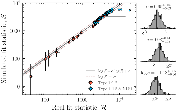
Figure 9: (Left) Posterior predictive checks showing the real fit statistics vs. simulated fit statistics for the highest Bayes Factor models per source with X-ray data, separated into type 1s and 2s with blue and red points, respectively. The straight line shown in dark grey and associated shading is the median posterior model line and associated posterior uncertainty. The dashed lines on either side of the median denote the intrinsic scatter in the vertical direction from the fit. (Right) from top to bottom shows the marginalised posterior for the straight line fit gradient, intercept and intrinsic scatter, respectively. Each marginalised distribution shows the mode with dark grey shading, together with the 95% highest density interval with light grey shading. The posterior straight line fit is consistent with a one-to-one relation on average for the entire sample, suggesting the majority of model fits are acceptable on average.

6.4 The Column Density Distribution

Having used a few different metrics to select models in Section 6.2, each source is allowed to have N line-of-sight $N_{\mathrm{H}}$ posterior distributions, where N is the number of suitable models per source, given their optical spectroscopic classification. Each accepted model then fits the observed spectra equally well within our assumed model selection thresholds. Incorporating every accepted model posterior per source is important, since individual $N_{\mathrm{H}}$ posterior distributions can differ in terms of not only quantiles but also shape. We specifically refer to the ability of different obscuring models fitting the same source with different posterior distributions as ‘geometry-dependent degeneracies’ (previously discussed in Yaqoob 2012; Brightman et al. 2015; LaMassa et al. 2019; Saha et al. 2022; Kallová et al. 2024). However, the ability of BXA to traverse a parameter space globally means that each accepted posterior for a given source should have a negligible if not non-existent effect from local minima. We hence assume that each BXA posterior represents a robust possible solution to explain a given set of observed source X-ray spectra, and attempt to include all possible solutions in the final log $N_{\rm H}$ distribution with a Hierarchical Bayesian Model (HBM).

The HBM we use is very similar in form to the histogram model with Dirichlet prior described in Section 3, but with line-of-sight $N_{\rm H}$ posteriors from our X-ray spectral fitting. The parameters of the parent model are the bin heights of the $N_{\rm H}$ distribution in unit dex bins from $N_{\rm H}$ = 10²⁰ – 10²⁴ cm^-2, and one two-dex wide Compton-thick bin with $N_{\rm H}$ = 10²⁴ – 10²⁶ cm^-2. We additionally performed a Monte Carlo simulation to incorporate systematic model dependencies (e.g., the choice of model setup, the obscuration geometry, model parameterisations) into the final distribution. We selected one random accepted line-of-sight $N_{\rm H}$ posterior per source and generated the $N_{\rm H}$ distribution 200 times before appending the HBM model chains together. After experimenting with different numbers of repeats, 200 was chosen since all sources were sampled after significantly fewer iterations than this. As detailed earlier, 20 additional type 2 sources in the sample did not have any X-ray spectral constraints. To predict the line-of-sight $N_{\rm H}$ for these sources, we applied our Monte Carlo HBM to just the type 2 sources in the sample with X-ray spectral constraints and used the resulting $N_{\rm H}$ distribution as the predicted posterior for each type 2 lacking X-ray spectra. By including the 20 sources lacking X-ray spectra self-consistently, we assume the remaining type 2s share the same characteristics as the existing type 2s with X-ray spectra. Since the type 2 $N_{\rm H}$ distribution is heavily skewed to $N_{\rm H}$ $>$ 10²³ cm^-2, the main effect of incorporating sources with no X-ray data is to marginally increase the obscured and Compton-thick fractions.

The corresponding $N_{\rm H}$ distribution we find with our Monte Carlo HBM is shown in Figure 10, with the individual fractions per bin given in Table 7. By plotting the inter-parameter dependencies of the HBM in Figure 10, we show there is no strong degeneracy between any bin fractions apart from the Compton-thin ($N_{\rm H}$ = 10²³ – 10²⁴ cm^-2) and the Compton-thick ($N_{\rm H}$ = 10²⁴ – 10²⁶ cm^-2) fractions which shows a slight negative correlation. Such a degeneracy indicates that a number of sources have $N_{\rm H}$ posteriors consistent with both obscuration classes, such that the overall Compton-thick fraction can only increase at the detriment of the Compton-thin fraction and vice-versa. This inter-bin fraction degeneracy also shows the benefit of our self-consistent fitting method, and shows the difficulty associated with defining sources as Compton-thick when too few obscurer geometries are considered in the modelling process.

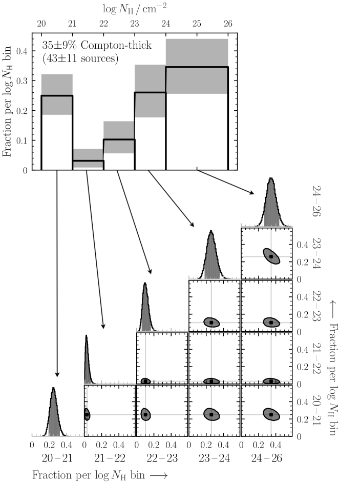
Figure 10: The NuLANDS $N_{\rm H}$ distribution. The result from the HBM described in Section 6.4 is shown here as a corner plot with each axis representing a different parameter 90% confidence range from the model (i.e. the bin heights in the $N_{\rm H}$ distribution). Each parameter is not strongly degenerate with one another, apart from a slight negative diagonal dependence between the Compton-thin ($N_{\rm H}$ = 10²³ – 10²⁴ cm^-2) and Compton-thick ($N_{\rm H}$ = 10²⁴ – 10²⁶ cm^-2) fractions. This highlights the power of our self-consistent method for deriving line-of-sight column densities. For a number of sources consistent with both classifications, a source can become Compton-thick so long as the Compton-thin fraction is reduced and vice-versa. Due to the range in maximum line-of-sight column density values allowed by each model considered, we choose to represent the Compton-thick fraction as a single two dex bin encompassing $N_{\rm H}$ = 10²⁴ – 10²⁶ cm^-2.

Table 7: NuLANDS $N_{\rm H}$ distribution fractions.

$N_{\rm H}$ bin boundaries / cm-2	Fraction per dex $\times$ bin width
1020 – 1021	$0.25^{+0.07}_{-0.06}$
1021 – 1022	$0.03^{+0.04}_{-0.02}$
1022 – 1023	$0.10^{+0.06}_{-0.05}$
1023 – 1024	$0.26^{+0.09}_{-0.08}$
1024 – 1026	$0.35\pm 0.09$

Note. — All fractions were calculating using the Monte Carlo Hierarchical Bayesian Model method described in Section 5 with results presented in Section 6.4 and Figure 10.

7 Discussion

7.1 The NuLANDS Column Density Distribution

The $N_{\rm H}$ distribution for the full NuLANDS sample is presented in Figure 10 as a one-dimensional histogram and a two-dimensional corner plot. The corner plot highlights the structure of the hierarchical model used to construct the $N_{\rm H}$ distribution, in which the fractions in each bin are the free parameters of the model. No strong correlations between individual bin fractions are found for most cases. The most notable parameter dependence between individual bin fractions is a slight negative trend between the Compton-thin ($N_{\rm H}$ = 10²³ – 10²⁴ cm^-2) and Compton-thick ($N_{\rm H}$ = 10²⁴ – 10²⁶ cm^-2) fractions. Such a trend indicates that a number of the AGN in NuLANDS have line-of-sight $N_{\rm H}$ posteriors from some proportion of the selected model fits that are consistent with both Compton-thin and Compton-thick classifications. Due to the lack of such trends between other bin fractions, the trend between Compton-thin and Compton-thick fractions highlights the overall difficulty, even with NuSTAR, to classify the line-of-sight column density with high precision when the source is heavily obscured and a single spectral model is being used for inference. A much weaker anti-correlation is visible between the unobscured ($N_{\rm H}$ = 10²⁰ – 10²¹ cm^-2) and Compton-thick fractions. Though unlikely to affect our final column density distribution, a negative trend could suggest a small number of sources with unobscured reprocessing signatures (e.g., from accretion disk and/or outflow-based reprocessing; Parker et al. 2022; Matzeu et al. 2022) that are being explained by high column density reprocessing in the circum-nuclear obscurer.

Of the full sample comprising 122 sources, we find a Compton-thick fraction of 35 $\pm$ 9% (equivalent to 43 $\pm$ 11 sources) with $N_{\rm H}$ = 10²⁴ – 10²⁶ cm^-2 where the fraction has been normalised to unity in the log $N_{\rm H}$ = 10²⁰ – 10²⁶ cm^-2 range. The NuLANDS Compton-thick fraction is thus fully consistent with the value found by Buchner et al. (2015) of 38${}^{+8}_{-7}$%, broadly consistent with the value found by Ananna et al. (2019) of 50 $\pm$ 9% up to redshift 0.1 within 90% confidence and the value found by Ueda et al. (2014) of $\sim$44%.

For intermediate obscuration levels, $N_{\rm H}$ = 10²² – 10²⁴ cm^-2, we find an increase in the fraction of sources from 10${}^{+6}_{-5}$% for $N_{\rm H}$ = 10²² – 10²³ cm^-2 to 26${}^{+9}_{-8}$% for $N_{\rm H}$ = 10²³ – 10²⁴ cm^-2. Interestingly, obscuration is expected to be partly explained by host-galaxy obscurers below $N_{\rm H}$ $\sim$ 10²³ – 10^23.5 cm^-2 (Buchner et al., 2017; Buchner & Bauer, 2017; Silverman et al., 2023), though with a strong dependence on redshift (Andonie et al., 2022). Compton-thick levels are unlikely to be produced by kpc-scale obscurers in all but the most extreme compact and luminous starbursts in the nearby universe (see e.g., Gilli et al. 2022; Andonie et al. 2024). Deriving properties of the host-galaxy obscurer and its connection with the central AGN requires comprehensive multi-wavelength contributions (e.g., García-Burillo et al. 2021), but is outside the scope of this paper. We note that if a majority of the NuLANDS obscured AGN were dominated by large-scale host galaxy obscurers, the isotropy tests between the mid-to-far infrared continuum and optical narrow line regions shown in Section 3 and Figure 3 would not be expected to agree so well between the type 1 and type 2 sources. Thus, such isotropy tests indicate the NuLANDS $N_{\rm H}$ distribution in Figure 10 is dominated by circum-nuclear rather than large-scale obscuration.

The overall shape of the one dimensional $N_{\rm H}$ distribution presents an apparent drop of sources with $N_{\rm H}$ = 10²¹ – 10²² cm^-2 from the much higher fraction of unobscured sources. Though a somewhat common feature of previous $N_{\rm H}$ distributions (see Section 7.3), we adhere caution to interpreting a decrease since an unknown fraction of the $N_{\rm H}$ = 10²⁰ – 10²¹ cm^-2 sources are $N_{\rm H}$ upper limits. The exact $N_{\rm H}$ upper limits are either limited by the minimum allowed $N_{\rm H}$ per fit (the lowest considered in the models is $N_{\rm H}$ = 10²⁰ cm^-2) or could be degenerate with the Galactic column density that was fixed in each fit. Since the Galactic $N_{\rm H}$ values used in this work (from Willingale et al. 2013) were distributed between $N_{\rm H}$ $\sim$ 10^20.0 – 10^21.3 cm^-2 (i.e. entirely encompassing the lowest column density bin of the $N_{\rm H}$ distribution), it is difficult to determine accurately how many sources could have intrinsic line-of-sight column densities $N_{\rm H}$ $<$ 10²⁰ cm^-2.

7.2 NuLANDS Column Density Dependencies

7.2.1 Distance

As noted earlier, a clear trend in hard X-ray all-sky flux-limited surveys of AGN is the decrease of the Compton-thick AGN fraction with distance (Ricci et al., 2015; Torres-Albà et al., 2021) due to an observational bias against heavily obscured sources. Since NuLANDS was constructed to select Compton-thick AGN with approximately equal efficacy as less-obscured AGN, it is important to test for a similar effect with distance in our sample. In Figure 11 we show the NuLANDS log $N_{\rm H}$ distribution for the entire sample (black contours) and for three different bins of distance. Within the 90% percentile range for each distribution (the shaded regions in the one-dimensional histograms), there is no significant change in the Compton-thick fraction. In addition, all other log $N_{\rm H}$ distribution bins are consistent within the 90% percentile range, suggesting that distance effects do not strongly affect the NuLANDS fitting results.

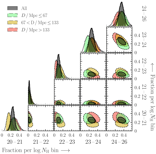
Figure 11: $N_{\rm H}$ distribution hierarchical model corner plot, binned by distance in Mpc. No significant deviations are observed with distance.

7.2.2 Total Infrared Luminosity

Higher galaxy total infrared luminosities can imply large quantities of dust on large galactic scales and/or merging/interacting systems. In the former scenario, large scale host-galaxy dust can lead to enhanced X-ray obscuration of AGN up to $N_{\rm H}$ $\sim$ 10^23.5 cm^-2 (Buchner et al., 2017). However, for merging/interacting systems, the material is thought to be funneled to the parsec-scale environment surrounding the supermassive black hole, simultaneously triggering star formation (e.g., Sanders et al. 1988) and enhancing circum-nuclear obscuration (e.g., Ricci et al. 2017b, 2021).

As discussed in Section 3, if a substantial fraction of the NuLANDS AGN had enhanced levels of large-scale host-galaxy dust obscuration, the isotropy tests highlighted in Figure 3 would not be expected to agree between type 1 and 2 AGN so well. As shown in Figure 12, we find no large disagreements between log $N_{\rm H}$ fractions within the 90% percentile range for the total NuLANDS sample (black) and binned by total infrared luminosity. Note that we also provide a total infrared luminosity-based estimate for star formation rate (SFR) using the relation from Kennicutt (1998).

The lack of large offsets for the $N_{\rm H}$ measurements with different total infrared luminosities provides further evidence that the NuLANDS selection can identify AGN isotropically. We include the corresponding translation from the total infrared luminosity bin edges to star formation rate in the legend of Figure 12 assuming the relation of Kennicutt (1998). Whilst this may indicate no strong relation between star formation rate and line-of-sight column density, we caution the reader that the presence of an AGN in the infrared can dramatically affect star formation rate estimations using that relation.

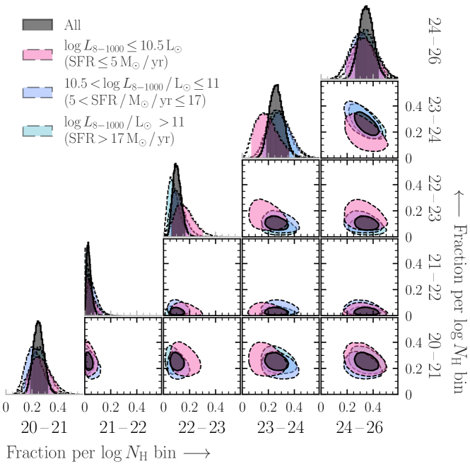
Figure 12: $N_{\rm H}$ distribution hierarchical model corner plot, binned by total infrared luminosity, log $L_{8-1000\mu{\rm m}}$. All $N_{\rm H}$ contours are consistent with the values found for the whole sample.

7.2.3 Near-to-Mid Infrared Colors

The NuLANDS AGN all satisfy a warm IRAS color classification, essentially a relatively steep mid-to-far infrared color in the 25–60 $\mu$m band. Such an AGN imprint on the observed spectrum above $\sim$25$\mu$m would be expected to correlate with similar infrared color selections at shorter wavelengths, for example in the near-to-mid-infrared. To date, many such near-to-mid infrared color selections exist for e.g., WISE (Jarrett et al., 2011; Stern et al., 2012; Mateos et al., 2012; Assef et al., 2018; Satyapal et al., 2018). To investigate such near-to-mid infrared color selections, and their possible effect on identifying log $N_{\rm H}$ for a given sample we apply a number of popular WISE color selections from the literature to the NuLANDS AGN.

In Figure 13 we report the NuLANDS log $N_{\rm H}$ distribution for AGN that are and are not selected based on the WISE color selections of Stern et al. (2012), Mateos et al. (2012) and Assef et al. (2018, we use the R90 selection specifically). We find that the majority ($>$ 60%) of NuLANDS AGN are identified as AGN based on all WISE color selections chosen, in broad agreement with their confirmed warm IRAS colors between 25–60 $\mu$m. For the AGN not selected, a likely reason is host galaxy dilution caused by star formation and other host galaxy-related processes dominating the bolometric output of the galaxy rather than the AGN (e.g., Murphy et al. 2009; Eckart et al. 2010; Mateos et al. 2013; Pfeifle et al. 2022).

We find consistent Compton-thick fractions for NuLANDS AGN both in and out of the WISE color selections considered. A similar trend was reported in Gandhi et al. (2015b) who found no clear preference for bona fide Compton-thick AGN in the local Universe across the WISE color-color space that were originally selected via a wide range of multi-wavelength methods. As expected, the largest uncertainties on log $N_{\rm H}$ bin fractions are found for AGN not selected by each WISE color criterion. This is likely a result of having more sources selected as AGN than not, and also that WISE color criteria are known to be more efficient for high X-ray luminosities often associated with AGN-dominated systems (e.g., Stern et al. 2012; Mateos et al. 2013). All $N_{\rm H}$ bin fractions are found to be consistent within 90 percentile contours, with some slight offsets observed. The largest log $N_{\rm H}$ bin fraction offsets are found for sources not selected as AGN with the 90% reliability (R90) cut of Assef et al. (2018), though note that of all NuLANDS AGN, the R90 cut is the most effective by selecting 82% of the NuLANDS sources. A possible link between the NuLANDS near-to-mid infrared spectral shapes and their X-ray column densities would require broadband spectral energy distribution decomposition, which is outside the scope of the current work. However, the general agreement between $N_{\rm H}$ bin fractions for NuLANDS AGN outside and inside a number of different WISE color selections provides further evidence for the isotropic nature of the NuLANDS selection.

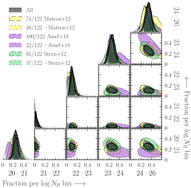
Figure 13: $N_{\rm H}$ distribution hierarchical model corner plot, binned by near-to-mid infrared WISE colors. No strong deviations are observed, whether in (solid lines) or out (dashed lines) of the selection criteria from Stern et al. (2012), Mateos et al. (2012), or Assef et al. (2018), indicating no strong relation between X-ray-derived $N_{\rm H}$ and star-formation contamination (which tends to preferentially affect near-to-mid infrared AGN color selection criteria).

7.2.4 AGN Optical Classification

Several previous works have found a correlation between optical spectral classification and X-ray-derived $N_{\rm H}$ above and below $\sim$10²² cm^-2. For example, Koss et al. (2017) find $\sim$94% agreement between Seyfert 1–1.8 and Seyfert 2 for X-ray $N_{\rm H}$ below and above a boundary of $\sim$ 10^21.9 cm^-2, respectively, in the Swift/BAT 70-month sample. Merloni et al. (2014) compare the X-ray and optical/UV classifications of the XMM-Newton COSMOS survey complete to observed X-ray flux, finding a substantial fraction of sources with unobscured/obscured X-ray classifications but the reverse in the optical/UV. The authors find that optically-classified type 2 AGN that are unobscured in X-rays are likely caused by host galaxy dilution, whereas for optically-classified type 1 AGN that are obscured in X-rays could be caused by dust-free gas within/inside the broad line region. For the latter cross-classification sources, the authors find the majority to be at relatively high intrinsic luminosity, which are likely less relevant in the volume-limited NuLANDS sample considered here. For the former class, this may be a possibility in a subset of the sources.

To test the possible presence of type 2 AGN that are X-ray unobscured, we plot the NuLANDS log $N_{\rm H}$ distribution for type 1–1.8 and type 1.9–2 in Figure 14. We find negligible fractions of type 2 AGN with unobscured X-ray spectra, though note this may be somewhat by design. Our X-ray model selection does allow neutral obscuration for type 1s, but we restrict the models accessible to either optical spectral class (i.e. physical torus models were only selected for optically-classified type 1.9–2 sources). Interestingly, the type 2 Compton-thick fraction of 49$\pm 12$% is fully consistent with the type 2 Compton-thick fraction of Kammoun et al. (2020), which may suggest that the vast majority of the type 2 AGN in our sample agree with their X-ray obscuration classification. Additionally, there are 20 type 2 AGN with no X-ray coverage that we assume an $N_{\rm H}$ prior for in our $N_{\rm H}$ distribution hierarchical model based on the type 2s with X-ray data. These missing sources may include sources with disagreeing optical and X-ray obscuration classification.

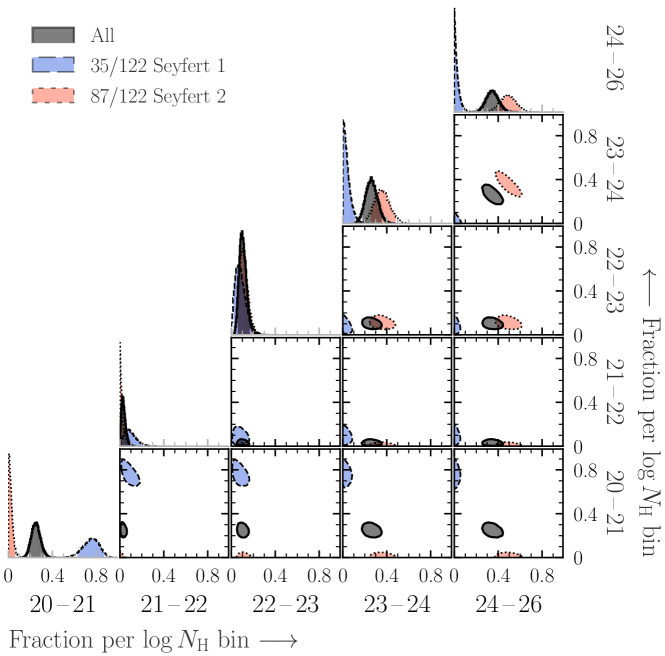
Figure 14: $N_{\rm H}$ distribution hierarchical model corner plot, binned by optical spectroscopic classification (Seyfert 1 = type 1–1.8; Seyfert 2 = type 1.9–2). A strong deviation is found between the two classifications, as expected from unification, and consistent with previous works.

7.2.5 Intrinsic X-ray Luminosity

Whilst the principle aim from our spectral fitting was to constrain the global line-of-sight column density for the local AGN population, the models we use all parameterise the intrinsic coronal X-ray continuum as a powerlaw with intrinsic normalisation and photon index as free parameters. We generate intrinsic (i.e. unabsorbed) X-ray luminosity posteriors in the 2–10 keV band for each source by integrating the equivalent powerlaw flux generated from the intrinsic normalisation and photon index posteriors. As such, all uncertainties are propagated into the intrinsic luminosity posterior.

To investigate trends between intrinsic luminosity and line-of-sight column density, we consider the luminosity posteriors for the highest Bayes Factor models per source only and also the mode of each posterior. We then split the NuLANDS $N_{\rm H}$ distribution corner plot into three sub-groups of intrinsic 2 – 10 keV luminosity, namely $L_{2-10\,{\rm keV}}$ $<$ 10⁴² erg s^-1, 10⁴² erg s^-1 $<$ $L_{2-10\,{\rm keV}}$ $<$ 10⁴³ erg s^-1 and $L_{2-10\,{\rm keV}}$ $>$ 10⁴³ erg s^-1, resulting in Figure 15. Although a single model is chosen for placing in a given intrinsic luminosity bin, the same Monte Carlo-derived column density distribution which considers all acceptable models per source is used to generate the $N_{\rm H}$ distribution. The process could thus result in some intrinsic luminosity posteriors that may not apply to some column density posteriors, but we expect such scenarios to be infrequent. Furthermore, using the same Monte Carlo technique as the other $N_{\rm H}$ distribution corner plots presented in this section enables a direct comparison since the same technique is used to model the parent line-of-sight column density distribution.

Of the full sample of 102 sources with X-ray data, we find 19 in which the highest Bayes Factor model gives an intrinsic luminosity posterior mode below 10⁴² erg s^-1. On manual inspection, a number of these sources are either low signal-to-noise, meaning that the intrinsic luminosity posterior is better explained by an upper limit or multi-modal with a lower portion of the intrinsic luminosity posterior mass above the 10⁴² erg s^-1 threshold. For this reason, these targets are marked with faint shading in Figure 15. Of the sources with higher predicted intrinsic luminosities, the two luminosity bins we consider give fully consistent column density distribution predictions. However, there are only four sources in our sample with $L_{2-10\,{\rm keV}}$ $>$ 10⁴⁴ erg s^-1; two type 1 sources (3C 120 and Mrk 509) and two Compton-thick type 2 sources (2MASX J15504152–0353175 and Mrk 573), implying a Compton-thick fraction that is still consistent with the entire NuLANDS column density distribution at the highest luminosities in the sample.

Previous works have found evidence for an effect between the fraction of obscured sources and the intrinsic X-ray luminosity (see e.g., Ricci et al. 2017c, Extended Data Figure 3). However, considering the relatively small fraction of higher-luminosity sources with e.g., $L_{2-10\,{\rm keV}}$ $>$ 10⁴⁴ erg s^-1, one would expect a reduced effect between covering factor and luminosity at these lower luminosities. For example, Brightman & Nandra (2011a) found the fraction of sources with $N_{\rm H}$ $>$ 10²² cm^-2 in the 12 $\mu$ Galaxy Sample to be broadly consistent with constant for intermediate intrinsic luminosities $L_{2-10\,{\rm keV}}$ $\sim$ 10⁴⁰ – 10⁴⁴ erg s^-1. Thus we may not see a strong effect between obscuration and luminosity because of the overall lower intrinsic luminosities of the sources in NuLANDS as compared to e.g., the Swift/BAT sample which contains a higher fraction of sources with $L_{2-10\,{\rm keV}}$ $>$ 10⁴⁴ erg s^-1. Though a stronger driver for feedback on the circum-nuclear obscurer of AGN seems to be the Eddington ratio (e.g., Fabian et al. 2008; Ricci et al. 2017c; Ananna et al. 2020, 2022; Ricci et al. 2022), due to the incompleteness of black hole mass estimates currently in the NuLANDS sample we defer such analyses to future work.

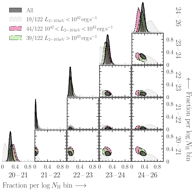
Figure 15: $N_{\rm H}$ distribution hierarchical model corner plot, binned by predicted intrinsic 2–10 keV luminosity from the highest Bayes Factor model fit per source. The binning was performed on the mode of the intrinsic luminosity posterior. Thus for $L_{2-10\,{\rm keV}}$ $<$ 10⁴² erg s^-1, the majority are upper limits on intrinsic luminosity caused by poorer quality spectral constraints.

7.3 Comparison with Other Local AGN Samples Observed in X-rays

Here we compare and contrast the results (primarily $N_{\rm H}$ distributions) with other local AGN samples in the literature.

7.3.1 Swift/BAT

A number of works have focused on careful $N_{\rm H}$ constraints for AGN detected by the all-sky Swift/BAT monitor. Ricci et al. (2017a) combined all 70-month Swift/BAT spectra between 14 – 195 keV for the 838 detected AGN with soft X-ray spectra from a number of complementary facilities to constrain line-of-sight $N_{\rm H}$ with a wide array of spectral models. The authors select a sample of 55 Compton-thick AGN candidates from their analysis (see Ricci et al. 2015 for more details of the targets), representing an observed Compton-thick fraction of 7.6${}^{+1.1}_{-2.1}$% out of all non-blazar AGN in the 70-month sample. After considering a number of luminosity and obscuration geometry-dependent bias corrections, Ricci et al. predict a bias-corrected Compton-thick fraction of 27$\pm$4% in the local Universe (normalised to unity in the $N_{\rm H}$ = 10²⁰ – 10²⁵ cm^-2 range), which is consistent with the Compton-thick fraction we find for the entire NuLANDS sample. The overall shape of the bias-corrected $N_{\mathrm{H}}$ distribution from Ricci et al. is also in general agreement with the NuLANDS distribution reported in this paper, suggesting the NuLANDS selection is complimentary to hard X-ray flux-limited selection by identifying Compton-thick AGN in a representative manner.

There have been numerous NuSTAR follow-up campaigns of Swift/BAT-detected Compton-thick AGN candidates. The largest NuSTAR legacy sample dedicated to observing BAT-detected obscured sources is detailed in Balokovic (2017); Baloković et al. (2020) who consider type 1.8, 1.9 and 2 AGN from the 70-month Swift/BAT compilation of Baumgartner et al. (2013). Sources were selected based on publicly-available NuSTAR data within a volume of $z$ $<$ 0.1 and with observed BAT fluxes $F_{\rm 14\,-\,195\,keV}$ $>$ 10^-11 erg s^-1 cm^-2. Balokovic uses an alternative approach to Ricci et al. (2015) to bias-correct the observed Compton-thick fraction in the sample. Different assumptions on the Compton hump strength (parameterized by rel_refl in the pexrav model) were assumed for the sample to reverse engineer the effective X-ray sensitivity with obscuration level. The resulting bias-corrected Compton-thick fraction (relative to the entire sample of unobscured and obscured AGN with the same selection steps as their sample) was $\gtrsim$ 27%, in very good agreement with the bias-corrected value from Ricci et al. (2015) as well as the observed fraction from NuLANDS.

Similar constraints have been acquired with NuSTAR follow-up of the deeper Swift/BAT Palermo 100-month catalog (Marchesi et al., 2018, 2019b; Traina et al., 2021; Torres-Albà et al., 2021). The most recent observed Compton-thick fraction from the sample is $\sim$ 8% when compared to all AGN selected within a volume of $z$ $\leq$ 0.05 (Sengupta et al., 2023), in agreement with Ricci et al. (2015) and Balokovic (2017). Zhao et al. (2021) then presents a Monte Carlo-based bias-correction using the best-fit geometrical parameters derived from physical torus modelling of the sample. At $\sim$ 37%, the predicted bias-corrected Compton-thick fraction with this method is higher than previous estimates using the 70-month BAT catalog (though it is still consistent with the lower limit from Balokovic 2017), and is in very good agreement with the observed fraction we find for NuLANDS.

More recently, Tanimoto et al. (2022) used the XCLUMPY model to analyze 52/55 of the original 70-month Swift/BAT-detected Compton-thick candidates from Ricci et al. (2015) with publicly-available NuSTAR data. Notably, the authors find that after incorporating NuSTAR data, 24 of the objects no longer have line-of-sight column densities consistent with the Compton-thick regime within 90% confidence. The reduction of Compton-thick AGN corresponds to a reduced observed Compton-thick fraction of $\sim$ 3.9% for the 70-month Swift/BAT non-blazar sample. Similar results highlighting the importance of NuSTAR data in disentangling parametric degeneracies and constraining line-of-sight column densities are reported in Marchesi et al. (2018, 2019b, 2019a). Such results highlight the benefit of comprehensive NuSTAR follow-up in deriving robust line-of-sight column density estimations for AGN in combination with sufficiently-sensitive spectral constraints in the soft band simultaneously (e.g., Molina et al. 2024).

7.3.2 CfA Seyferts

The CfA Seyfert sample was derived from the parent CfA Redshift Survey (Huchra et al., 1983), 2399 galaxies with optical spectroscopy that is complete down to a limiting galaxy magnitude of $m_{\rm Zw}$ $\leq$ 14.5 mag. Of the galaxies in the CfA Redshift Survey, Huchra & Burg (1992) selected a complete sub-sample of 27 Seyfert 1s and 21 Seyfert 2s (48 Seyferts total) within the magnitude limit of the CfA Redshift Survey. Huchra & Burg additionally estimated the Seyfert 2 to Seyfert 1 ratio from the sample to be 2.3$\pm$0.7, since for a given galaxy optical brightness, an intrinsically powerful AGN would always be preferentially detected if a type 1 as opposed to a type 2.

Of the 21 Seyfert 2s from the CfA Seyfert sample, 12 were observed by NuSTAR as part of the Swift/BAT sample follow-up, NuLANDS or other targeted observations. The remaining 9/21 Seyfert 2s from the CfA Seyfert sample that had not been previously observed were selected for a NuSTAR Legacy Survey (PI: J. Miller; Kammoun et al. 2020). Of the nine Seyferts observed by NuSTAR, Kammoun et al. ruled out two sources as Seyfert 2s (NGC 5256 and Mrk 461) based on follow-up optical spectroscopy that placed the targets in the composite star-forming $+$ Seyfert region of the [N ii]/H$\alpha$ vs. [O iii]/H$\beta$ BPT diagram, leaving 19 Seyfert 2s in total.

Kammoun et al. fit phenomenological (featuring pexmon) and physical (featuring coupled and decoupled variations of MYtorus) models to the 19 targets in the sample, finding between 6 – 10 of those Seyfert 2s to be Compton-thick depending on the choice of model and archival results. The resulting observed Compton-thick fraction out of the full 19 Seyfert 2s $+$ 27 Seyfert 1s = 46 CfA Seyfert sample (albeit neglecting $N_{\rm H}$ measurement uncertainty) is then between 14${}^{+10}_{-7}$ – 23${}^{+11}_{-9}$% which is below but consistent with the NuLANDS 90% confidence range within uncertainties. However, if we correct the Seyfert 2 to Seyfert 1 ratio of the CfA Seyfert sample based on the predicted ratio from Huchra & Burg (1992) of 2.3 $\pm$ 0.7, assuming the same fraction of missing Seyfert 2 sources to be Compton-thick as found by Kammoun et al., we calculate a bias-corrected prediction for the Compton-thick fraction to lie in the range of $\sim$ 22${}^{+8}_{-7}$ – 37${}^{+9}_{-8}$% for the CfA Seyfert sample. Such a range is in good agreement with the observed value from NuLANDS. As described earlier, Seyfert 2s are expected to be preferentially missed in optical spectroscopic classifications relative to Seyfert 1s at a given optical flux level, since the continuum is typically more suppressed in the former relative to the latter.

7.3.3 The Complete 15 Mpc Sample

As discussed in Section 1.2, near-to-mid infrared lines produced in the narrow line region do not suffer considerably from line-of-sight extinction. The Complete 15 Mpc Sample (Annuar et al., in prep.) is one such local universe selection, originating from the [Ne v] mid-infrared line selection of Goulding & Alexander (2009). The parent sample is the Revised Bright Galaxy Sample from IRAS (Sanders et al., 2003), which selects the brightest sources detected by IRAS with 60$\mu$m flux densities $f_{60\mu{\rm m}}$ $>$ 5.24 Jy. A very local volume cut was imposed on the sample of 15 Mpc, from which 19 galaxies were selected as AGN based on significant [Ne v] emission in their Spitzer Space Telescope (Werner et al., 2004) high resolution infrared spectra. The [Ne v] line has a high excitation potential, making its production unlikely from pure stellar systems. Of the 20 sources, eight were selected as part of a NuSTAR program, though X-ray data is available for all, including an additional 17 with NuSTAR data. To date, NuSTAR has helped robustly confirm two of the sample as Compton-thick AGN: NGC 5643 (Annuar et al., 2015) and NGC 1448 (Annuar et al., 2017), as well as NGC 660 with line-of-sight column density solutions both below and above the Compton-thick threshold (Annuar et al., 2020). The sample has additionally identified a number of genuine low-luminosity AGN with 2 – 10 keV luminosities $L_{2-10\,{\rm keV}}$ $\lesssim$ 10⁴¹ erg s^-1, providing further evidence that [Ne v] is an extremely effective indicator of AGN activity with little contamination from stellar processes.

Other than NGC 1068, there is no overlap in sources between the [Ne v] sample and NuLANDS. Firstly, NGC 1068 is the only source in our sample at a distance $<$ 15 Mpc. But this and the very small overlap with NuLANDS is likely caused by the difficulty of producing warm 25-to-60 $\mu$m continuum shapes (as required by the NuLANDS selection) when the AGN component is a small fraction of the overall bolometric luminosity of the host galaxy. Low AGN-to-host bolometric fractions are found for the [Ne v] sample with many systems having observed X-ray luminosities $L_{2-10\,{\rm keV}}$ $<$ 10⁴² erg s^-1 (Annuar et al., in prep.).

7.3.4 The 12 Micron Galaxy Sample (12MGS)

The 12MGS (Spinoglio & Malkan, 1989) was derived from the IRAS PSCv2 with (co-added) 12$\mu$m flux densities $f_{12\mu{\rm m}}$ $>$ 0.3 Jy. The authors show that typical AGN spectra are broadly isotropic in the mid-infrared, with the 12$\mu$m flux being approximately one-fifth of the bolometric value for all Seyfert types. The extended 12MGS (Rush et al., 1993) then used the IRAS Faint Source Catalog Version 2 to derive an alternative selection of 893 galaxies with a lower flux limit of 0.22 Jy at 12$\mu$m.

The most comprehensive X-ray follow-up of the 12MGS was reported by Brightman & Nandra (2011b, a), who analysed all publicly-available XMM-Newton data of the sample as of 2008-December (126 sources with meaningful spectra). Brightman & Nandra (2011a) find a Compton-thick fraction of 20$\pm$4% in the X-ray luminous ($L_{2-10\,{\rm keV}}$ $>$ 10⁴² erg s^-1) sub-sample, which included optically-classified non-AGN. Though below that of NuLANDS, the 12MGS Compton-thick fraction would likely increase with increased hard X-ray coverage, so this Compton-thick fraction is likely a lower limit.

A number of AGN selected in the 12MGS have been observed by NuSTAR to date. La Caria et al. (2019) consider three 12MGS Seyfert galaxies with observed differences between the infrared and X-ray bolometric luminosities of up to three orders of magnitude, finding all targets to be heavily obscured and two to be Compton-thick. Saade et al. (2022) alternatively selected a sample of nine Seyfert 2 AGN from the 12MGS with observed 2–10 keV luminosities significantly below that of their observed [O iii] luminosities to investigate the possibility of X-ray obscuration or faded AGN. Using NuSTAR data, three galaxies were confirmed to be Compton-thick, with four of the remaining sources being heavily obscured.

7.3.5 The Great Observatories All-sky LIRG Survey (GOALS)

Similar to the Complete 15 Mpc sample of Goulding & Alexander (2009), GOALS (Armus et al., 2009) is fundamentally derived from the Revised Bright Galaxy Sample (Sanders et al., 2003), but instead selects all Luminous InfraRed Galaxies (LIRGs, 181 sources) and Ultra-Luminous InfraRed Galaxies (ULIRGS, 21 sources), giving a total sample size of 202 sources at a median distance of 94.8 Mpc and $z$ $\leq$ 0.088. Owing to the bright infrared selection of the sample, a large fraction of the sources are confirmed interacting systems (Armus et al., 2009).

To date there has been extensive X-ray coverage of the GOALS sample. Iwasawa et al. (2011) analysed the Chandra data for a complete sub-sample of 44 bright GOALS sources with log $L_{8-1000\,\mu{\rm m}}$ $>$ 11.73 L_⊙, finding X-ray detections for all but one target. Considering all sources with hard X-ray colors, a detected 6.4 keV iron line and a confirmed mid-infrared [Ne v] line, the total detected AGN fraction was 48%. Koss et al. (2013) presented a targeted hard X-ray survey of local GOALS-selected LIRGs with Swift/BAT, finding 40 $\pm$ 9% of the sample to have 14 – 195 keV / 2 – 10 keV band ratios consistent with high or Compton-thick line-of-sight column densities predicted from the MYtorus model. Torres-Albà et al. (2018) then investigated the Chandra data for a lower luminosity sub-sample of 63 GOALS sources, finding a consistent fraction of X-ray-confirmed AGN to the higher luminosity sources analysed in Iwasawa et al. (2011).

To constrain the line-of-sight column density, Ricci et al. (2017b) considered all GOALS sources with publicly-available NuSTAR data as of 2016-March that were confirmed to be interacting, as well as three systems detected by Swift/BAT but not observed by NuSTAR. All 30 systems in the sample were found to be obscured with $N_{\rm H}$ $>$ 10²³ cm^-2, implying a large covering factor for all sources. After additionally binning the sample by observed merger stage, the authors find early-stage mergers to have a Compton-thick fraction of 35${}^{+13}_{-12}$%, consistent with the bias-corrected value of Ricci et al. (2015) as well as the value we report for NuLANDS here. In contrast, for the late-stage mergers in the sample a higher Compton-thick fraction of 65${}^{+12}_{-13}$% is observed, which is significantly higher than we find for NuLANDS.

Ricci et al. (2021) consider an extended sample of 60 GOALS systems observed by NuSTAR, fitting the confirmed AGN with the RXtorus X-ray spectral model (Paltani & Ricci, 2017; Ricci & Paltani, 2023). The authors find a similarly enhanced Compton-thick fraction in late-stage mergers of 74${}^{+14}_{-19}$%. Complementary X-ray spectral fitting of 57 GOALS sources with publicly-available NuSTAR data or 105-month Swift/BAT data was performed by Yamada et al. (2020, 2021). For the 30 sources detected in the hard X-ray band, the authors fit with XCLUMPY and find Compton-thick fractions of 24${}^{+12}_{-10}$% and 64${}^{+14}_{-15}$% in early and late-stage mergers, respectively, fully consistent with the findings of Ricci et al. (2017b, 2021).

7.4 Comparison with Population Synthesis Models

As described throughout this paper, the fraction of Compton-thick AGN amongst the AGN population is currently highly uncertain and a source of significant systematic uncertainty in population synthesis models. Representative samples such as NuLANDS should provide excellent benchmarks for model evaluation. In this sub-section, we compare the observed Compton-thick fraction from NuLANDS to the values predicted across a number of different population synthesis models in the literature as well as other hard X-ray-based analyses of local AGN samples discussed earlier in this Section.

In Figure 16, we collate the predicted Compton-thick fractions from five population synthesis models in the literature that each use different methodologies and AGN selection functions: Gandhi & Fabian (2003), Gilli et al. (2007), Ueda et al. (2014), Buchner et al. (2015) and Ananna et al. (2019). The model by Gandhi & Fabian (2003) was based on a mid-infrared selection approach for tackling obscuration selection bias of type 2 AGN, and results therein were one of the original motivations behind the NuLANDS selection. The remaining four models are all popular population synthesis studies in the literature that each use X-ray selected samples, and we defer the reader to the individual papers for specific information regarding each model. For models that do not report uncertainties on the Compton-thick fraction, we assume a default uncertainty of 10% which is typical of the median luminosity function uncertainties for the samples used. But it should be kept in mind that systematic uncertainties related to model assumptions could be higher; these are non-trivial to compare in a self-consistent manner, but some first insights are possible from the scatter across the model predictions.

For any models that report an evolution of the Compton-thick fraction with luminosity we make sure to report the fraction relevant for intrinsic luminosities $L_{2-10\,{\rm keV}}$ $\lesssim$ 10⁴³ erg s^-1 where possible to match the approximate expected intrinsic luminosities of the NuLANDS sample (see Section 7.2.5 and Figure 15). We then compare each model prediction for the Compton-thick fraction to the measured (and bias-corrected where available) Compton-thick fractions in qualitatively similar luminosity ranges from the following hard X-ray local AGN analyses: the NuSTAR-based analysis of Kammoun et al. (2020) (including the completeness-corrected range derived in Section 7.3.2), the 70-month BAT analyses of Ricci et al. (2015) and Balokovic (2017) and the latest estimates from the ongoing 100-month Palermo BAT (NuSTAR-based) analysis of Sengupta et al. (2023).

Figure 16 clearly shows that from the five population synthesis models considered, only NuLANDS finds a directly-observed Compton-thick fraction that is consistent with all population synthesis model-predicted values within uncertainties. When considering the bias-corrected values from other surveys, the completeness-corrected fraction for the CfA Seyfert sample (Kammoun et al., 2020) is consistent with all models at the upper range of possible Compton-thick fractions. The general agreement between the predicted completeness-corrected Compton-thick fraction in the CfA Seyfert sample and the directly-observed NuLANDS sample provides additional support that the NuLANDS selection is representative of type 1 and type 2 AGN.

In terms of Swift/BAT-selected samples, the observed Compton-thick fractions from Ricci et al. (2015) and Sengupta et al. (2023) out to further distances than NuLANDS are inconsistent with all the models considered. The highest observed fraction from BAT-selection that is plotted in Figure 16 is from the lowest redshift bin of z $<$ 0.01 ($D_{L}$ $\lesssim$ 45 Mpc) in the NuSTAR-based follow-up of the 100-month Palermo BAT sample (Torres-Albà et al., 2021; Sengupta et al., 2023). Similar results are reported by Ricci et al. (2015) for the 70-month sample, finding observed Compton-thick fractions within $\sim$ 50 Mpc that are broadly consistent with NuLANDS within errors but inconsistent with the model predictions of Ueda et al. (2014), Buchner et al. (2015) and Ananna et al. (2019). In terms of bias-corrected values, the lower limit prediction derived by Balokovic (2017) from an analysis of 70-month BAT-selected type 2 AGN is consistent with all models.

The overall consistency between NuLANDS and previous population synthesis models highlights NuLANDS as an optimized sample for future AGN surveys. We note that the largest discrepancy for NuLANDS is with the latest model of Ananna et al. (2019), offering tantalizing evidence that the NuLANDS obscured and Compton-thick fractions could still be a lower limit, in agreement with the sample bias considerations discussed in Section 3.

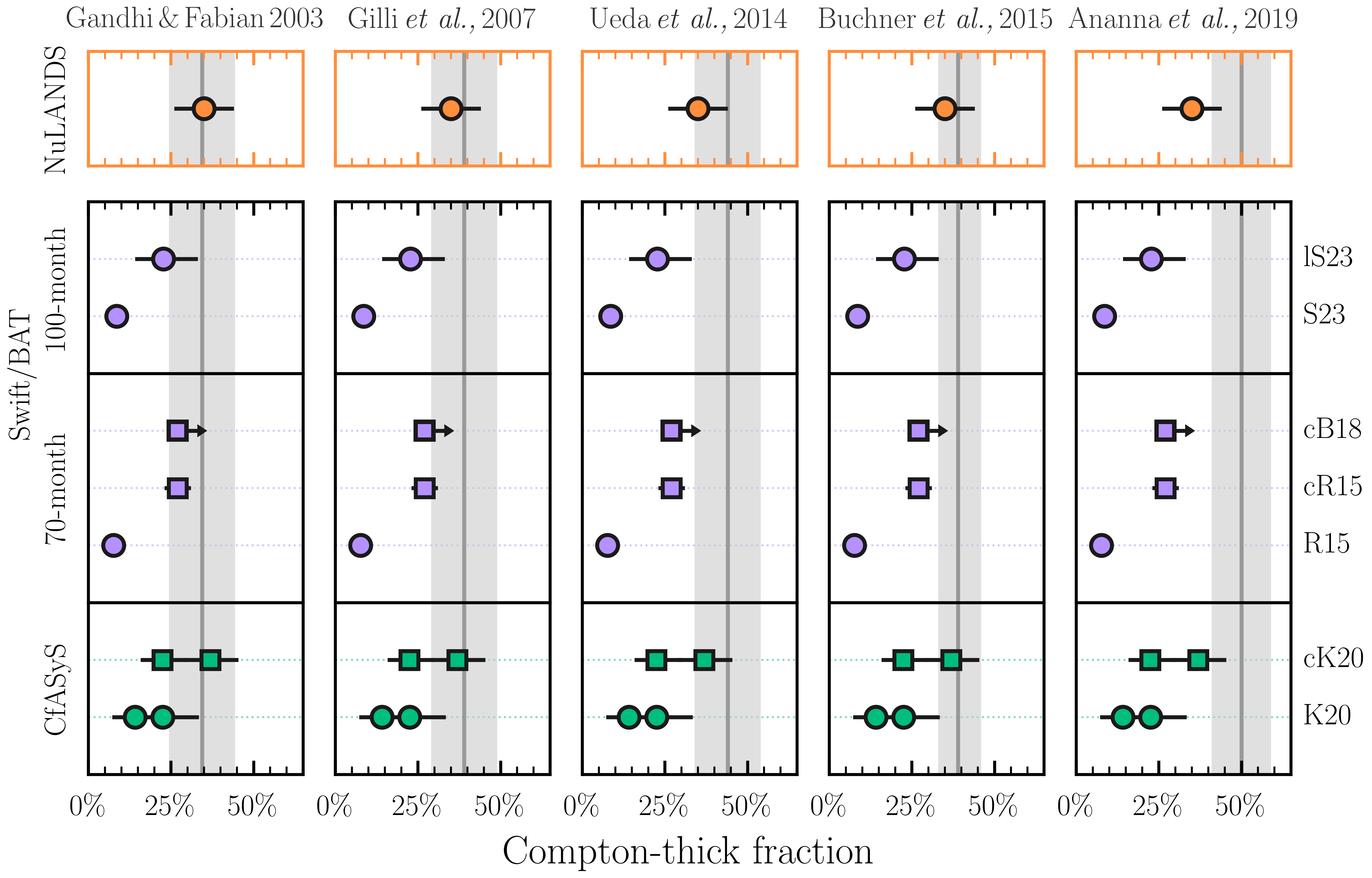
Figure 16: A compilation of Compton-thick AGN fractions derived in hard X-ray local AGN sample analyses compared to numerous population synthesis models from the literature. From bottom to top, the Compton-thick fractions are: K20; Kammoun et al. (2020), cK20; the completeness-corrected value derived in Section 7.3.2, R15; the observed fraction from Ricci et al. (2015), cR15; the bias-corrected value from Ricci et al. (2015), cB18; the bias-corrected value from Balokovic (2017), and S23/lS23; the observed fraction within $z$ $\leq$ 0.05/z $\leq$ 0.01 from the latest 100-month Palermo BAT sample of Sengupta et al. (2023), respectively. From left to right, the population synthesis models considered are from Gandhi & Fabian (2003), Gilli et al. (2007), Ueda et al. (2014), Buchner et al. (2015) and Ananna et al. (2019).

7.5 Variability

The soft X-ray observations analysed in this work were selected to be as quasi-simultaneous with NuSTAR as possible per source (see Section 4 for a breakdown). However, it is not unexpected for variability to affect the log $N_{\rm H}$ distribution results presented in this work to some degree (see Ricci & Trakhtenbrot 2023 for a recent review). Several studies have found obscuration variability in both type 1 and 2 AGN (e.g., Malizia et al. 1997; Risaliti et al. 2002; Kara et al. 2021), as well as between Compton-thin and thick obscuration levels which could affect our understanding of the Compton-thick fraction (e.g., Risaliti et al. 2005; Rivers et al. 2015; Ricci et al. 2016; Pizzetti et al. 2022; Marchesi et al. 2022; Torres-Albà et al. 2023; Lefkir et al. 2023; Pizzetti et al. 2024).

To make a preliminary assessment of any variability effects present in the observations analysed in this work, we use the cross-calibration constant for each model fit. Although cross-calibrations are supposed to account purely for instrumental effects when multi-instrument fits are performed, the posterior for the cross-calibration constant between FPMA and the soft X-ray instruments can be used to indicate the possible presence of variability to zeroth order. Figure 17 presents the median and 68th percentile range cross-calibration constants for all model fits selected for sources with joint NuSTAR and soft X-ray constraints as a function of the time difference of their respective observations. The median cross-calibrations are distributed as log $\mathcal{C}$ = -0.03$\pm$0.07, fully consistent with unity and also the cross-calibration constants determined by Madsen et al. (2015). The two sources with the highest cross-calibrations are KUG 0135–131 and IC 3639, though both still have values $\lesssim$ 2. There are also a number of XMM-Newton/EPN-based fits with cross-calibration values of $\sim$80% relative to NuSTAR/FPMA. As stated in the XMM-Newton calibration technical note, such large cross-calibration differences are not unexpected.

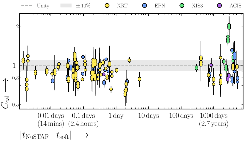
Figure 17: The difference between the start time of each NuSTAR and soft X-ray observation per source analysed in this sample vs. the cross calibration found in the spectral fitting for each model that is selected per source. No large evidence for variability in the sample is observed, with general agreement for each source with unity. The two offsets at large times are both type 2 AGN, and are discussed in Section 7.5.

7.6 Testing Sample Biases on the Column Density Distribution

7.6.1 Powerful AGN Missed by NuLANDS

NuLANDS is not designed to be a complete AGN population down to a fixed intrinsic luminosity, such that a number of bolometrically powerful AGN that are detected by IRAS are also missed by the warm IRAS mid-to-far infrared color classification. Two famous examples are NGC 4051 and NGC 6240, which both have $\alpha_{25,60}$ values indicative of cooler infrared spectra than we select. In this sub-section we check for any possible bias imposed on the $N_{\rm H}$ distribution (and Compton-thick fraction) by comparing a subset of the NuLANDS warm AGN to correspondingly cool mid-to-far infrared AGN. Our comparison sample is Swift/BAT since this is an efficient selector of bolometrically-luminous AGN ($L_{\rm bol}$ $\sim$ 10⁴⁴ – 10⁴⁶ erg s^-1) in the local universe provided the line-of-sight column density $N_{\rm H}$ $\lesssim$ 10²⁴ cm^-2.

To ensure as relevant a comparison for NuLANDS as possible, we match the 70-month Swift/BAT catalogue to the IRAS Point Source Catalogue v2.1 with a 1 arcmin matching radius, giving 331 matches. The choice of matching radius may introduce some mis-matches, but chance coincidence with contaminants is unlikely. In addition, since we are interested in population demographics, so long as a suitably large number of sources is considered in any single case, any such mis-matches should not introduce a systematic bias in a given column density bin over another. We then performed the same selection method as NuLANDS, namely removing low Galactic latitudes, the Magellanic Clouds and any sources with upper limits from IRAS at 25 $\mu$m or 60 $\mu$m. Finally we performed the same warm IRAS color selection between 25 and 60 $\mu$m to classify warm and correspondingly cool sources, giving 60 warm and 53 cool sources.

For consistency, the X-ray derived $N_{\rm H}$ values for each of the Swift/BAT warm and cool IRAS sources used the values derived in Ricci et al. (2017a). Using the $N_{\rm H}$ values from our analysis for the warm sources would likely increase the $N_{\rm H}$ distribution uncertainties for the warm sample (as opposed to the cool sample) since our analysis incorporates multiple model solutions per source. For each source, we use the torus model-derived $N_{\rm H}$ estimate from Ricci et al. (2017a) if available or the standard pexrav-derived value if not. We then convert the 90% uncertainties on $N_{\rm H}$ to 68% assuming a standard Gaussian distribution conversion before approximating the $N_{\rm H}$ parameter posteriors per source by a two-piece Gaussian distribution to incorporate asymmetric errorbars. Finally, we use the same PosteriorStacker method as with the main NuLANDS $N_{\rm H}$ distributions to construct a parent histogram distribution for both the warm and cool Swift/BAT sources. The corresponding corner plot for the parent distributions are shown in Figure 18.

We find remarkable agreement in the Compton-thick fraction between warm and cool Swift/BAT sources, with values of 26${}^{+10}_{-9}$% and 28$\pm$10% for the warm and cool sources, respectively. All remaining $N_{\rm H}$ fractions below the Compton-thick limit are consistent between warm and cool sources within 90% confidence, though with some offsets. The observed offsets do not follow an obvious trend with higher fractions for warm sources in the $N_{\rm H}$ = 10²⁰ – 10²¹ cm^-2 and 10²³ – 10²⁴ cm^-2 bins vs higher fractions for cool sources in the 10²¹ – 10²² cm^-2 and 10²² – 10²³ cm^-2 bins. Such a lack of trend is indicative of stochastic effects dominating the $N_{\rm H}$ distribution fractions as opposed to some systematic bias in the selection process itself, though quantifying any such effects is outside the scope of this paper.

Finally, we note there are a number of Swift/BAT AGN not detected by IRAS, which we have not considered here. Quantifying the effect of AGN not included in NuLANDS due to non-detections from IRAS cannot be easily tested in the same manner (e.g., by investigating the $N_{\rm H}$ distribution of AGN detected by Swift/BAT but not IRAS) since both instruments have their own unique selection functions.

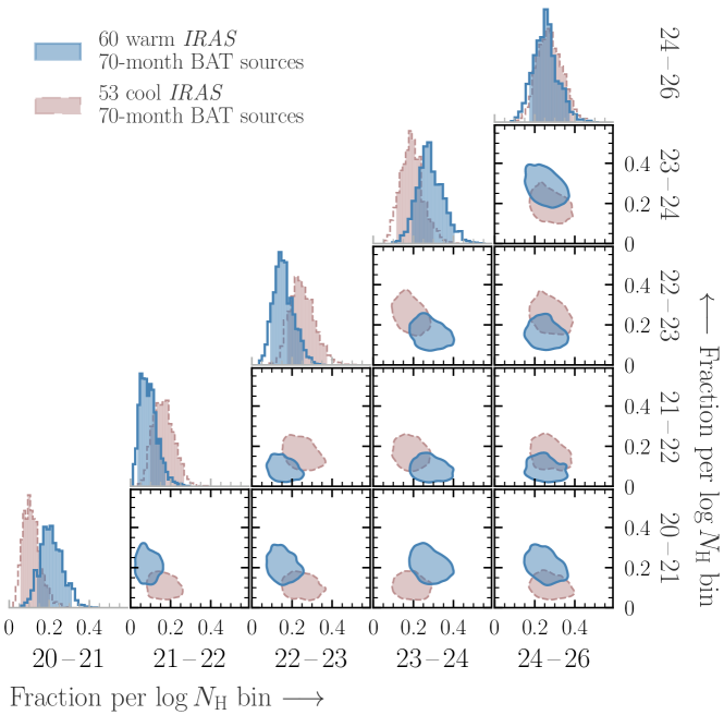
Figure 18: The log $N_{\rm H}$ distribution for the 70-month BAT sample, after identifying warm IRAS sources in the sample, selected and classified as AGN in the same way as for NuLANDS. ‘Cool’ IRAS sources are those which are not selected as warm based on their 25–60 $\mu$m spectral shape. All contours are consistent within 90%, with the strongest correspondence arising for the Compton-thick fraction.

7.6.2 Elusive AGN Missed by NuLANDS

As discussed earlier, the derivation of the NuLANDS sample includes optical spectroscopic classifications which can be affected by significant large-scale dust reddening (e.g., Goulding & Alexander 2009; Greenwell et al. 2021, 2022, 2024a). If missed, such elusive AGN would be predominantly associated with type 2 AGN due to the overall fainter continuum in such sources. From Figure 14, if a substantial number of such sources were missed in NuLANDS, a reduced number of Type 2 AGN would potentially increase the overall obscured fraction we report. To search for a possible dearth of Seyfert 2 AGN in our sample, we plot the type 1 and type 2 ratios as a function of distance in the left panel of Figure 19. A reduced overall number of type 2 AGN could be identified by a drop in the overall type 2 fraction with distance, or alternatively an increase in the type 1 ratio with distance. Neither effect is observed, with each bin being fully consistent with the total type 1 and type 2 fractions from the entire sample.

An additional test is shown in the right panel of Figure 19, in which the fractions of sources in incremental two dex bins of X-ray-derived $N_{\rm H}$ from Figure 11 are plotted in the same format as the left panel versus distance. A similar trend is observed, in which all fractions are found to be consistent with the values found for the entire sample.

Nevertheless the possibility of elusive AGN missed by the optical spectral classifications still remains, meaning that the obscured fraction for NuLANDS can be conservatively considered a lower limit. It is not implausible for a significant number of the HII-classified galaxies to contain Compton-thick AGN. In the subset of sources studied by Moran et al. (2002), 11/18 targets were found to display normal galaxy optical spectra, four of which ($\sim$36%) have since been confirmed as Compton-thick with NuSTAR-based analyses (NGC 1358; Marchesi et al. 2022, NGC 2273; Masini et al. 2016, NGC 3982; Saade et al. 2022 and NGC 5347; Kammoun et al. 2019). In principle one could test the hypothesis of a substantial fraction of obscured elusive AGN by comparing the host galaxy inclination distribution to the full underlying galaxy population distribution. Such comparisons would require careful consideration of a variety of possible biases, which is outside the scope of this work.

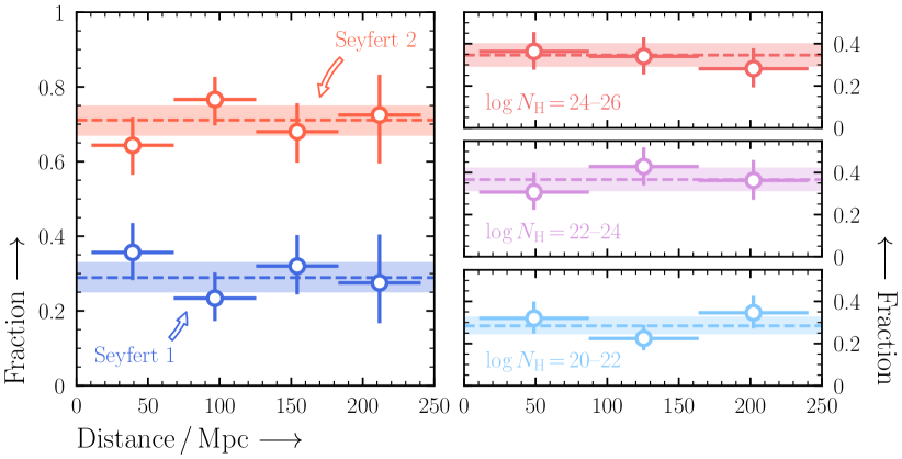
Figure 19: Left: The type 1 and type 2 fractions in NuLANDS as a function of distance. For both types, the fraction in each bin of distance is consistent within uncertainties of the average for the whole sample, shown with dashed lines and 68th percentile shading. Right: The fraction of sources in particular log $N_{\rm H}$ bins from the $N_{\rm H}$ distribution as a function of distance. All fractions are consistent with the values for the whole sample (shown with dashed lines and 68th percentile shading), as expected for an isotropically selected sample.

7.6.3 AGN Types Preferentially Selected by NuLANDS

Owing to the requirement for Point Source Catalogue v2.1 detections at 60 $\mu$m, the NuLANDS selection is flux-limited to $F_{60\,\mu{\rm m}}$ $\gtrsim$ 0.5 Jy. Other far-infrared flux-limited surveys (with albeit higher flux thresholds) often find large fractions of Ultra/Luminous InfraRed Galaxies (U/LIRGs) (e.g., Kewley et al. 2001; Sanders et al. 2003) which are found to be far more obscured on average relative to e.g., the Swift/BAT AGN sample (e.g., Koss et al. 2013; Ricci et al. 2017b, 2021). Thus a preferential selection of U/LIRGs in NuLANDS would likely lead to an enhanced obscured and Compton-thick fraction relative to the underlying AGN population.

As outlined in Section 3 and Figure 3, the flux ratios between [O iii] and the 25 and 60 $\mu$m fluxes for type 1s and type 2s indicate that a strong preference for dusty systems is not present in the sample, possibly partly due to the requirement for detected AGN-dominated [O iii] emission in the first place. A sample with considerable contamination from U/LIRGs would likely include a large contribution from large-scale host galaxy dust reddening in the optical (e.g., Veilleux et al. 1995, 1999).

For a more quantitative test for the presence of U/LIRGs in NuLANDS, we compare with the GOALS sample. As detailed in Section 7.3.5, the GOALS sample contains a complete LIRG subset of the Revised IRAS Bright Galaxy Sample within a volume of $z$ $<$ 0.088 (approximately twice the volume of NuLANDS). We determine how many GOALS sources have warm 25 – 60 $\mu$m spectra using the same classification as NuLANDS. Out of a total 202 GOALS sources, 7 have mid-to-far infrared spectral slopes consistent with NuLANDS – the remainder have much colder spectral slopes. Of the 7 matches, one is excluded since it has flux upper limits at 25 and 60 $\mu$m (VV 414) and a further two (IRAS 05223+1908 and NGC 1275) are excluded since the Galactic latitudes are outside that of the NuLANDS cut (see Section 2). Of the remaining four sources, one (the late-stage merger ESO 350-IG 038) is classified as an optical HII galaxy and thus not included in this work. Ricci et al. (2021) recently reported the 22.6 ks NuSTAR non-detection of this source, finding the Chandra spectrum to be described well with a pure star-forming component and no hard X-ray component. The final three sources are in the NuLANDS sample and included in this paper, consisting of two confirmed Compton-thick AGN – NGC 1068 (Bauer et al., 2015), NGC 7674 (Gandhi et al., 2017) – and a Compton-thin AGN – MCG -03-34-064 (Ricci et al., 2017a).

Figure 20 plots the NuLANDS, Swift/BAT and GOALS samples in the plane of 25-to-60 $\mu$m color vs. total infrared 8 – 1000 $\mu$m luminosity derived using the relation from Sanders & Mirabel (1996). The 25 – 60 $\mu$m color range used to classify warm IRAS sources is shown with a vertical shaded region. For a fair comparison with NuLANDS, we used fluxes reported in the IRAS point source catalog for all sources. Since the NuLANDS selection did not exclude flux upper limits at 12 or 100 $\mu$m and the point source catalog contained a number of flux upper limits in one or more IRAS bands for other sources, a number of the values plotted in Figure 20 are upper limits. We note that the total infrared luminosity is limited by the requirement for IRAS detections, such that the Swift/BAT data could potentially extend to lower luminosities than is plotted. However, good agreement is found between Swift/BAT and NuLANDS indicating that the warm IRAS color criterion is capable of identifying AGN efficiently. The lack of cross-over with GOALS is somewhat more revealing in this plot however, since the GOALS sources are found to be at systematically higher luminosities and significantly cooler mid-to-far infrared colors than NuLANDS. Such cooler colors are associated with mid-to-far infrared spectral energy distributions peaking at colder temperatures than a typical AGN, which indicates a dominant contribution from the host galaxy in the 25 – 60 $\mu$m spectra for the majority of GOALS sources. Indeed AGN are typically very difficult to identify in the GOALS sample owing to the strong nuclear obscuration and contamination from the host galaxy (Iwasawa et al., 2011; Torres-Albà et al., 2018; Vardoulaki et al., 2015; Díaz-Santos et al., 2017; Falstad et al., 2021). Nevertheless Figure 20 indicates that U/LIRGs typically occupy a different region of the mid-to-far infrared color vs. total infrared luminosity plane than NuLANDS, which suggests that the Compton-thick and obscured AGN fractions are not significantly boosted by a strong presence of such systems in the sample.

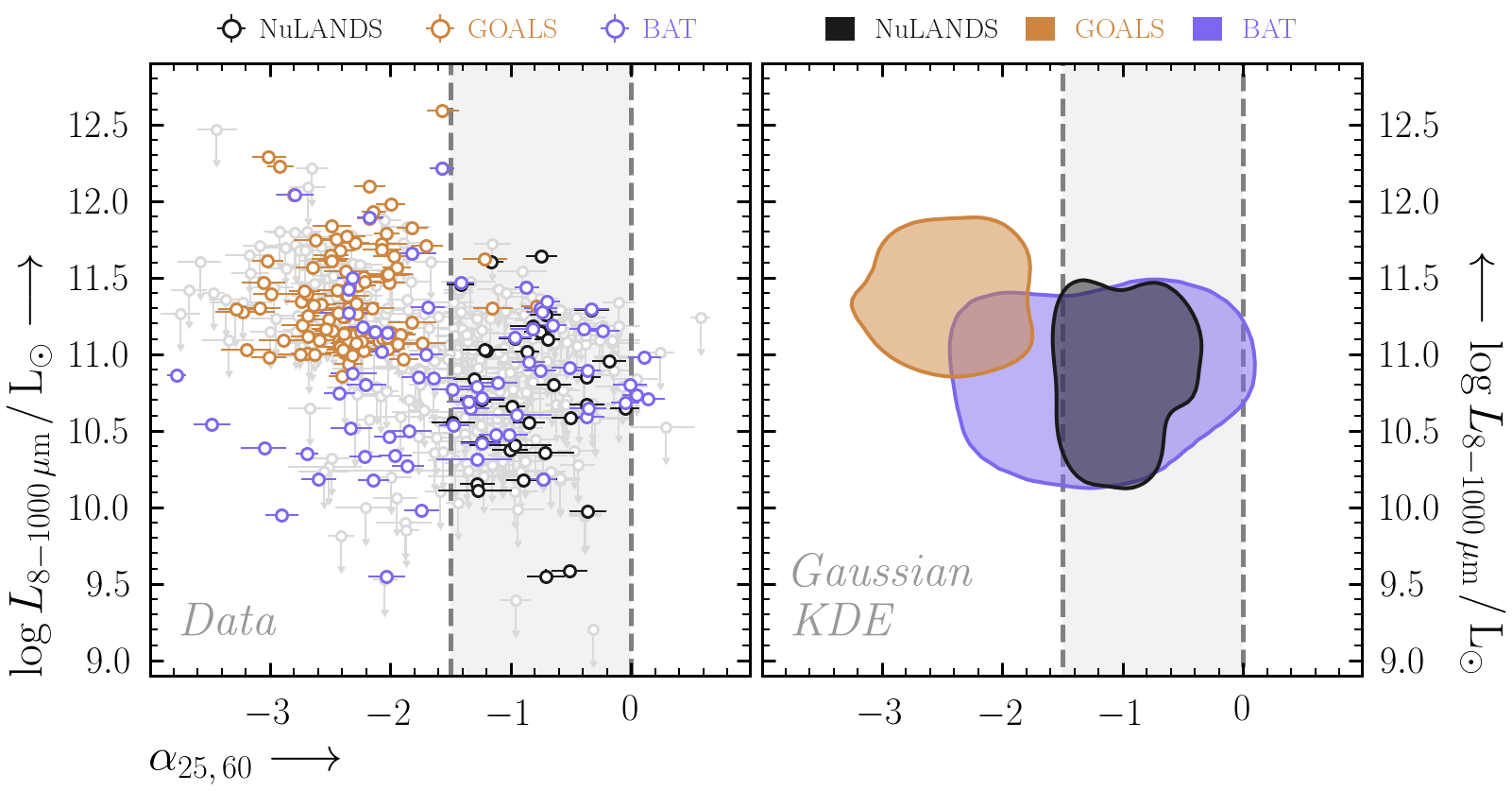
Figure 20: Mid-to-far infrared spectral slope (parameterised with $\alpha_{25,60}$) vs. total infrared luminosity, $L_{8-1000\,\mu{\rm m}}$ for the NuLANDS, GOALS and BAT samples. NuLANDS occupies a distinct area of the parameter space to that of GOALS, likely due to a reduced number of host galaxy-dominated mid-to-far infrared systems. Interestingly NuLANDS occupies a similar parameter space to BAT, indicating that NuLANDS does not over sample infrared-bright sources on average. The NuLANDS warm mid-to-far infrared spectral color is shown with a vertical shaded region bounded by dashed lines. Left and right panels show the same data, displayed in different ways for clarity. Left shows the detections with colored errorbars, and the upper limits are shown in grey in the background. Right shows a Gaussian Kernel Density Estimation containing 68% of each dataset, including upper limits as detections.

7.7 Outlook and Prospects for Broadband X-ray Spectroscopy of Local AGN

Robust Compton-thick classifications require robust constraints above 10 keV by definition to include the underlying reprocessed continuum. The majority of the Compton-thick sources revealed in this paper are too faint for any instrument but NuSTAR to do this. However, a subset of the Compton-thick candidates are still faint enough to yield upper limits on the observed X-ray continuum at high energies (see Section 7.2.5). In such cases, BXA is able to yield robust upper limits on intrinsic X-ray luminosity, but the line-of-sight column density posteriors likely allow a wide range of values. The High Energy X-ray Probe (HEX-P) is a probe-class mission concept proposed for launch in 2032 (Madsen et al., 2024). The HEX-P design includes two telescopes, one Low Energy Telescope (LET) operating between 0.2 – 25 keV and a High Energy Telescope (HET) operating between 2 – 80 keV. Together, the LET and HET provide simultaneous broadband X-ray spectra with dramatically improved spectral sensitivity relative to both XMM-Newton and NuSTAR combined. HEX-P thus holds promise for studying AGN in a wide variety of ways, from black-hole spins of large populations (Piotrowska et al., 2024), unveiling the physics of the corona (Kammoun et al., 2024), probing the circum-nuclear environment of heavily obscured and Compton-thick AGN (Boorman et al., 2024), understanding the demographics of obscured AGN across cosmic time (Civano et al., 2024) and studying the nature of dual AGN in exquisite detail (Pfeifle et al., 2024).

To showcase the importance of HEX-P for the NuLANDS sample in modelling the reprocessed continua of faint heavily obscured AGN in our sample, we select five of the faintest heavily obscured NuLANDS targets. To enable a like-for-like comparison with HEX-P, load the corresponding NuLANDS model P7 fit per source (based on the UXCLUMPY model) and simulate 200 ks of operational time using the same background and response files as the real observation. For HEX-P, we simulate the same best-fit model with the LET and HET, using the current best estimate response files (v07 - 17-04-2023). However, due to an overall factor of $\sim$ 2 improvement in observing efficiency relative to NuSTAR (Madsen et al., 2024), 200 ks of operational time with HEX-P is equivalent to 200 ks of exposure on-source compared to 100 ks with NuSTAR.

Figure 21 presents the corresponding simulated NuSTAR (3 – 78 keV) and HEX-P (0.2 – 80 keV) spectra, plotted in folded units normalised by the effective area and scaled logarithmically. over for NuSTAR and 0.2 – 80 keV bandpass provided by the LET and HET combined. HEX-P is able to reproduce the underlying reprocessed continuum from each AGN and thermal component in a single observation, enabling true broadband spectral modelling without any issues arising from non-simultaneous variability effects. In addition, the LET and HET provide sensitive overlapping spectra over the spectral range associated with the inflection point of the Compton hump between $\sim$ 8 – 24 keV, which has been shown to be critical in deciphering the nature of the circum-nuclear obscurer in detail (Buchner et al., 2019).

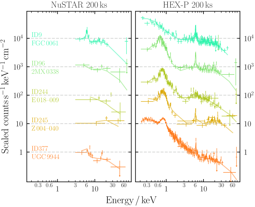
Figure 21: Comparing the current capabilities with NuSTAR (left column) to those of the High Energy X-ray Probe (HEX-P, right column) with five of the faintest heavily obscured candidates in the NuLANDS sample. Each spectrum is scaled logarithmically by their model flux at 5 keV and plotted in folded units normalised by the effective area. All spectra were simulated for 200 ks of operational time and then binned visually to have a minimum signal-to-noise ratio of three per bin. We note that 200 ks of operational time with NuSTAR is equivalent to 100 ks once Earth occultations are accounted for. However, there is no such exposure correction for HEX-P due to improved observing efficiencies (see Madsen et al. 2024 for more information). See Section 7.7 for more details of the simulations and Figure 5 for definitions of source identifier abbreviations.

8 Summary and Conclusions

In this work, we present the first paper from the NuSTAR Local AGN $N_{\rm H}$ Distribution Survey (NuLANDS). NuLANDS is an X-ray legacy survey of a mid-to-far infrared selected sample of AGN in the nearby universe ($z$ $<$ 0.044). NuLANDS was constructed to sample optically-classified type 1 AGN with approximately equal efficacy as optically-classified type 2 AGN, with the ultimate goal of providing a sample of AGN that is selected isotropically in terms of line-of-sight column density.

We fit a large library of 23 individual models to each source and check the column density distributions arising from each (Section 6.2). Following a Bayesian framework, our fitting process is automated with the PyMultiNest nested sampling implementation in BXA (Buchner et al., 2014). Our key findings are as follows:

1. Isotropic selection: We demonstrate that NuLANDS is isotropically selected based on indistinguishable flux ratios of [O iii] to the mid-to-far infrared 25 and 60 $\mu$m continuum emission for the optically-classified type 1 and 2 AGN (Section 3 and Figure 3). This means that derived quantities, like the distribution of line-of-sight obscuring column density, are closer to the intrinsic distribution than what is seen in X-ray-selected samples.

2. Significant model dependencies: We show that the choice of spectral model can have significant effects on the parent line-of-sight column density distribution derived for a given sample of sources with X-ray spectral fitting (Section 6.1). For sources not selected in the 70-month BAT catalog, we find that the line-of-sight column density can vary on average by a factor of $\sim$ 1.4 orders of magnitude between different models, reaching $>$ 2 orders of magnitude in extreme cases (Section 6.2, Tables 11 and 11). To overcome such issues, we develop a Monte Carlo-based Hierarchical Bayesian Model that conservatively propagates the systematic uncertainties associated with individual models into the parent column density distribution for the entire sample (Section 6.4).

3. The column density distribution: We find a Compton-thick fraction of 35 $\pm$ 9% to 90% confidence (35 $\pm$ 6% to 68% confidence), which is consistent with the latest estimates from the population synthesis model of Ananna et al. (2019) as well as many previous estimates (e.g., Ueda et al. 2014; Buchner et al. 2015). We discuss sample selection and classification biases, suggesting our obscured fraction could still be a lower limit.

4. Constant selection with distance: We find no significant systematic trends in any column density distribution bins with distance. Notably, the Compton-thick fraction does not significantly diminish with increased distance out to $\sim$ 200 Mpc.

5. Luminosity dependence: No significant effect is found for the Compton-thick fraction as a function of total infrared luminosity in the 8 – 1000 $\mu$m wavelength range. Using the Kennicutt (1998) relation, we correspondingly find no trend between the Compton-thick fraction and star formation rate though note that AGN contamination may affect our inference of star formation rates derived from infrared fluxes. We additionally find no increase in the Compton-thick fraction with intrinsic luminosities 10⁴² $<$ $L_{2-10\,{\rm keV}}$ $<$ 10⁴³ erg s^-1 and $L_{2-10\,{\rm keV}}$ $>$ 10⁴³ erg s^-1 within 90% confidence.

6. Tests for sample biases: We find no significant difference in the column density distribution between the warm and cool IRAS AGN selected from the Swift/BAT sample, indicating that any bolometrically-luminous AGN missed by NuLANDS are not missed in a manner biased against column density measurements (Section 7.6.1). We additionally compare the NuLANDS selection to that of GOALS, finding a significant difference in the infrared properties used to select either sample (Figure 20). Our findings suggest that NuLANDS does not select a disproportionate amount of U/LIRGs that could enhance the obscured and/or Compton-thick fractions of the sample (Figure 20 and Section 7.3.5).

The relatively high Compton-thick fraction reported here is in line with recent estimates that take into account biases against finding the most heavily obscured AGN, and is significantly higher than some older estimates. This implies a much larger fraction of supermassive black hole accretion that is missed by traditional optical and even X-ray surveys. Our work underlines the requirement for pairing multi-wavelength selection and classification techniques with sensitive broadband X-ray spectroscopy in the pursuit of an AGN census.

Appendix A Tables

=12mm

Table 8: Source properties of all optically-confirmed AGN in the NuLANDS sample, ordered by R. A.

IDa	NEDb	Simbadc	R. A.d	Dec.e	Morph.f	Inc.g	Typeh	Ref.i	$z^{j}$	Ref.k	$D^{l}$	log $N_{\rm H,\,Gal.}$ m
– Type 1 AGN (S1n, S1, S1.2, S1.5, S1.8) –
27	MRK 0359	MRK 359	21.885	19.179	S0	45.47	S1n	VV10	0.017390	NED	78.5	20.71
47	NGC 0931	NGC 931	37.060	31.312	Sbc	81.28	S1.0	VV10	0.016650	NED	48.0∗	20.95
54	NGC 0985	NGC 985	38.658	-8.788	I	45.21	S1.5	VV10	0.043140	NED	198.4	20.54
114	2MASS J04145265–0755396	2E 955	63.719	-7.928	$\cdots$	$\cdots$	S1.5	VV10	0.038160	NED	174.9	20.83
132	3C 120	MRK 1506	68.296	5.354	S0	65.05	S1.5	VV10	0.033010	NED	150.7	21.29
139	MRK 0618	MRK 618	69.093	-10.376	SBb	43.53	S1.0	VV10	0.035550	NED	162.6	20.76
160	2MASX J05014863–2253232	2MASX J05014863–2253232	75.453	-22.890	$\cdots$	30.07	S1n	VV10	0.040800	NED	187.3	20.41
171	ARK 120	MRK 1095	79.048	-0.150	E	51.78	S1.0	VV10	0.032710	NED	138.2∗	21.15
174	ESO 362– G 018	ESO 362–18	79.899	-32.658	S0-a	70.93	S1.5	VV10	0.012440	NED	55.9	20.26
209	IC 0450	IC 450	103.051	74.427	S0-a	63.19	S1.5	VV10	0.018810	NED	95.0∗	20.99
220	MRK 0009	MRK 9	114.238	58.770	S0	29.50	S1.5	VV10	0.039870	NED	182.9	20.75
225	UGC 03973	MRK 79	115.637	49.810	Sb	36.74	S1.2	VV10	0.022000	Hale	135.2∗	20.82
227	UGC 04013	MRK 10	116.871	60.934	SABb	67.82	S1.0	VV10	0.029000	Hale	82.4∗	20.75
233	IC 0486	IC 486	120.087	26.614	SBa	44.01	S1	VV10	0.026870	NED	119.0∗	20.57
260	MRK 1239	MRK 1239	148.080	-1.612	E	$\cdots$	S1n	VV10	0.019930	NED	90.1	20.65
278	NGC 3516	NGC 3516	166.705	72.573	S0	36.93	S1.5	NED	0.008840	NED	39.6	20.61
286	NGC 3783	NGC 3783	174.757	-37.739	SBa	26.65	S1.5	VV10	0.009730	NED	47.8∗	21.15
292	NGC 4253	NGC 4253	184.610	29.813	SBa	47.19	S1n	VV10	0.012930	NED	58.2	20.28
301	NGC 4593	NGC 4593	189.914	-5.344	Sb	34.03	S1.0	VV10	0.008344	Simbad	31.9∗	20.31
309	NGC 4748	NGC 4748	193.052	-13.415	S?	51.48	S1n	VV10	0.014630	NED	65.9	20.62
322	ESO 383– G 018	ESO 383–18	203.359	-34.015	Sb	90.00	S1.8	VV10	0.012410	NED	55.8	20.69
324	ESO 383– G 035	ESO 383–35	203.974	-34.296	Sab	58.78	S1.2	NED	0.007750	NED	34.7	20.68
344	NGC 5548	NGC 5548	214.498	25.137	S0-a	41.42	S1.5	VV10	0.017170	NED	35.8∗	20.21
350	UGC 09412	MRK 817	219.092	58.794	S0-a	24.59	S1.5	VV10	0.031450	NED	108.0∗	20.07
359	MRK 0841	MRK 841	226.005	10.438	E	$\cdots$	S1.5	VV10	0.036420	NED	166.7	20.39
369	UGC 09826	UGC 9826	230.387	39.201	SBc	51.95	S1.5	VV10	0.029440	NED	74.3∗	20.22
390	UGC 10120	MRK 493	239.790	35.030	Sb	55.68	S1n	VV10	0.031330	NED	54.0∗	20.36
398	IC 1198	IC 1198	242.152	12.331	SBab	63.45	S1.5	VV10	0.033660	NED	170.0∗	20.64
473	ESO 140– G 043	ESO 140–43	281.225	-62.365	SBbc	72.61	S1.5	VV10	0.014180	NED	50.9∗	20.98
484	ESO 141– G 055	ESO 141–55	290.309	-58.670	Sb	52.40	S1.2	VV10	0.037110	NED	169.9	20.81
497	NGC 6860	NGC 6860	302.195	-61.100	SBb	57.99	S1.5	VV10	0.015250	Simbad	68.7	20.56
509	MRK 0509	MRK 509	311.041	-10.724	$\cdots$	36.44	S1.5	VV10	0.034400	NED	240.5∗	20.71
531	ESO 344– G 016	ESO 344–16	333.675	-38.806	Sb	43.66	S1.5	VV10	0.039710	NED	182.2	20.11
537	MRK 0915	MRK 915	339.194	-12.545	Scd	67.00	S1.8	VV10	0.024110	NED	109.4	20.82
538	UGC 12138	UGC 12138	340.071	8.054	SBa	19.90	S1.8	VV10	0.024970	NED	113.3	20.95
– Type 1.9 AGN –
64	2MASX J02560264–1629159	2MASS J02560264–1629155	44.011	-16.488	$\cdots$	33.49	S1.9	VV10	0.03159	NED	144.1	20.60
68	NGC 1194	NGC 1194	45.955	-1.104	S0-a	71.50	S1.9	VV10	0.01360	NED	61.2	20.90
354	CGCG 164–019	2MASX J14453684+2702060	221.404	27.035	S0-a	$\cdots$	S1.9	VV10	0.02990	NED	136.2	20.43
495	2MASX J20005575–1810274	IRAS 19580–1818	300.232	-18.174	S0	60.23	S1.9	VV10	0.03700	Hale	169.4	21.05
548	NGC 7479	NGC 7479	346.236	12.323	SBbc	43.04	S1.9	VV10	0.00794	NED	27.7∗	20.89
– Type 2 AGN(S1h, S1i, S2, S) –
4	2MASX J00183589–0702555	2MASX J00183589–0702555	4.650	-7.049	E	90.00	S2	Hale	0.018000	Hale	81.3	20.58
9	FGC 0061	2MFGC 403	8.681	-0.041	Sb	83.90	S2	VV10	0.042200	NED	193.9	20.40
16	NGC 0262	NGC 262	12.196	31.957	S0-a	68.00	S1h	VV10	0.015030	NED	21.5∗	20.86
24	NGC 0424	NGC 424	17.865	-38.083	S0-a	78.48	S1h	VV10	0.011760	NED	50.7∗	20.21
26	NGC 0449	NGC 449	19.030	33.089	SBa	60.80	S2	VV10	0.015950	NED	71.9	20.81
30	KUG 0135–131	2MASX J01380539–1252105	24.522	-12.870	S0-a	54.30	S2	VV10	0.040210	NED	184.5	20.22
33	MRK 0573	MRK 573	25.991	2.350	S0-a	26.74	S1h	VV10	0.017180	NED	77.5	20.43
37	2MASX J01500266–0725482	ICRF J015002.6–072548	27.511	-7.430	$\cdots$	42.58	S1h	VV10	0.018030	NED	81.4	20.34
52	IC 1816	IC 1816	37.962	-36.672	SBab	15.23	S2	VV10	0.016950	NED	76.5	20.45
53	UGC 02024	UGC 2024	38.255	0.421	SBab	59.78	S2	VV10	0.022340	NED	101.2	20.35
57	NGC 1068	M 77	40.670	-0.013	Sb	34.70	S1h	VV10	0.003810	Simbad	10.5∗	20.51
63	2MASX J02553438+0223417	2MASX J02553438+0223417	43.893	2.395	$\cdots$	42.59	S2	Hale	0.028000	Hale	127.4	21.03
67	MCG –02–08–039	MCG –02–08–039	45.128	-11.416	Sa	55.85	S2	NED	0.029890	NED	127.0∗	20.79
70	2MASX J03023999–7242231	6DFGS GJ030240.0–724223	45.667	-72.706	$\cdots$	32.28	S2	NED	0.043460	NED	199.9	20.82
72	NGC 1229	NGC 1229	47.045	-22.960	SBbc	56.44	S2	VV10	0.036290	NED	166.1	20.26
75	2MFGC 02636	2XMM J031308.7–024319	48.287	-2.722	SABa	90.00	S2	Simbad	0.028290	NED	128.7	20.81
78	KUG 0312+013	2MASX J03150536+0130304	48.772	1.508	$\cdots$	57.24	S2	VV10	0.024020	NED	108.9	20.97
83	NGC 1320	NGC 1320	51.203	-3.042	Sa	80.53	S2	VV10	0.008880	NED	37.7∗	20.64
85	ESO 116– G 018	ESO 116–18	51.221	-60.739	S0-a	90.00	S2	VV10	0.018500	NED	83.6	20.56
96	2MASX J03381036+0114178	2MASX J03381036+0114178	54.543	1.238	$\cdots$	63.94	S2	NED	0.039780	NED	182.5	21.00
98	IRAS 03362–1641	LEDA 13422	54.640	-16.538	Sab	82.58	S2	NED	0.036900	NED	168.9	21.00
103	2MASX J03512799–0312099	6DFGS GJ035128.0–031210	57.867	-3.203	$\cdots$	57.10	S2	Hale	0.028000	Hale	127.4	21.15
122	2MASX J04250311–2521201	2MASX J04250311–2521201	66.263	-25.356	S0-a	66.29	S2	Simbad	0.041830	NED	192.2	20.63
141	2MASX J04405494–0822221	IRAS 04385–0828	70.229	-8.373	S0-a	82.23	S1h	VV10	0.014000	Hale	63.0	20.92
154	2MASX J04524451–0312571	IRAS 04502–0317	73.186	-3.216	S0-a	90.00	S2	Hale	0.016000	Hale	72.1	20.64
156	CGCG 420–015	2XMM J045325.7+040342	73.357	4.062	E	$\cdots$	S2	VV10	0.029390	NED	133.8	20.92
157	ESO 033– G 002	ESO 33–2	73.995	-75.541	S0	29.96	S2	VV10	0.018100	NED	81.7	21.10
168	ESO 362– G 008	ESO 362–8	77.788	-34.393	S0	81.07	S2	VV10	0.015750	NED	71.0	20.45
179	ESO 253– G 003	ESO 253–3	81.325	-46.006	Sa	65.00	S2	VV10	0.042490	NED	195.3	20.61
175	GALEXASC J052821.01+761708.4	IRAS 05212+7614	82.087	76.286	$\cdots$	$\cdots$	S2	Hale	0.037000	Hale	169.4	21.16
194	AM 0602–575	2MASX J06002140–5756210	90.089	-57.939	E	$\cdots$	S2	VV10	0.038150	Simbad	174.8	20.73
195	2MASX J06080957+6733394	2MASX J06080957+6733394	92.040	67.561	$\cdots$	$\cdots$	S2	Hale	0.017000	Hale	76.7	21.04
196	UGC 03426	MRK 3	93.901	71.037	S0	35.67	S1h	VV10	0.013510	NED	57.9∗	21.19
201	VII ZW 073	2MASX J06302561+6340411	97.606	63.678	$\cdots$	$\cdots$	S2	VV10	0.041330	NED	189.8	20.97
219	NGC 2410	NGC 2410	113.759	32.822	Sb	80.61	S2	VV10	0.015610	NED	63.5∗	20.71
224	MRK 0078	MRK 78	115.674	65.177	$\cdots$	49.47	S2	VV10	0.037000	Hale	169.4	20.59
226	UGC 03995B	UGC 3995 B	116.038	29.247	$\cdots$	$\cdots$	S2	VV10	0.015970	NED	58.6∗	20.64
236	UGC 04229	MRK 622	121.921	39.004	Sb	34.20	S2	VV10	0.023230	NED	105.3	20.77
244	ESO 018– G 009	ESO 18–9	126.033	-77.783	Sc	34.27	S2	NED	0.017820	NED	80.5	21.01
245	CGCG 004–040	2MASX J08301445–0252494	127.560	-2.881	Sab	48.30	S2	VV10	0.040560	NED	186.2	20.54
246	MRK 0093	MRK 93	129.176	66.233	Sa	48.41	S2	Hale	0.017000	Hale	76.7	20.69
253	MCG –01–24–012	MCG –01–24–012	140.193	-8.056	SABc	66.60	S2	VV10	0.019640	NED	88.8	20.53
263	KUG 1021+675	2MASX J10251299+6717493	156.304	67.297	Sc	0.00	S2	VV10	0.038600	NED	176.9	20.31
270	CGCG 333–049	MCG +12–10–067	161.036	70.405	Sb	66.92	S2	VV10	0.033580	NED	153.4	20.45
272	NGC 3393	NGC 3393	162.098	-25.162	SBa	30.94	S2	VV10	0.012510	NED	56.3	20.90
281	IRAS 11215–2806	IRAS 11215–2806	171.011	-28.388	Sb	79.23	S2	VV10	0.013990	NED	63.0	20.86
282	ESO 439– G 009	ESO 439–9	171.848	-29.258	SBab	80.49	S2	VV10	0.023890	NED	108.0∗	20.83
293	NGC 4388	NGC 4388	186.445	12.662	SBb	90.00	S1h	VV10	0.008420	NED	18.1∗	20.46
299	NGC 4507	NGC 4507	188.903	-39.909	Sab	32.45	S1h	VV10	0.011907	Simbad	53.5	20.98
302	IC 3639	IC 3639	190.220	-36.756	SBbc	21.76	S1h	VV10	0.011018	Simbad	49.5	20.87
306	NGC 4704	NGC 4704	192.193	41.921	SBbc	20.23	S2	VV10	0.027130	NED	105.0∗	20.12
310	ESO 323– G 032	ESO 323–32	193.335	-41.636	S0-a	42.66	S2	NED	0.016000	NED	72.1	21.08
312	NGC 4903	NGC 4903	195.345	-30.935	Sc	35.56	S2	VV10	0.016460	NED	61.5∗	20.92
313	NGC 4968	NGC 4968	196.775	-23.677	S0	90.00	S2	NED	0.009860	NED	44.3	21.09
314	2MASX J13084201–2422581	PKS 1306–241	197.175	-24.383	$\cdots$	69.96	S2	VV10	0.013930	NED	62.7	21.09
317	MCG –03–34–064	MCG –03–34–064	200.602	-16.728	S0	57.15	S1h	VV10	0.016540	NED	76.2∗	20.81
329	NGC 5347	NGC 5347	208.324	33.491	Sab	45.28	S2	VV10	0.007790	NED	21.2∗	20.20
341	NGC 5506	NGC 5506	213.312	-3.208	SABa	90.00	S1i	VV10	0.005890	Simbad	24.7∗	20.69
347	SBS 1426+573	2MASX J14281793+5710187	217.075	57.172	Sc	36.98	S2	VV10	0.042840	NED	197.0	20.10
348	2MASX J14312974–0317546	2MASX J14312974–0317546	217.874	-3.298	$\cdots$	80.15	S2	Hale	0.042000	Hale	193.0	20.82
349	2MASX J14344546–3250326	IRAS 14317–3237	218.689	-32.842	E?	46.58	S2	Simbad	0.025990	NED	118.1	20.85
352	MRK 0477	MRK 477	220.159	53.504	S0	51.34	S2	VV10	0.037730	NED	172.8	20.04
367	CGCG 077–080	2MASX J15205324+0823491	230.222	8.397	S0-a	65.45	S2	VV10	0.030920	NED	141.0	20.44
370	CGCG 077–117	2MASX J15241259+0832412	231.052	8.545	Sab	46.85	S2	VV10	0.037090	NED	45.9∗	20.49
377	UGC 09944	UGC 9944	233.949	73.451	Sbc	79.60	S2	VV10	0.024530	NED	111.3	20.50
379	CGCG 166–047	2MASX J15435731+2831269	235.989	28.524	SBbc	$\cdots$	S2	VV10	0.032180	NED	146.8	20.40
383	2MASX J15504152–0353175	IRAS 15480–0344	237.673	-3.888	E	53.22	S1h	VV10	0.030300	NED	138.1	21.29
447	CGCG 112–010	MCG +03–45–003	263.891	20.796	Sbc	34.79	S	VV10	0.024320	NED	110.3	20.97
461	NGC6552	NGC 6552	270.030	66.615	SBab	49.02	S1h	VV10	0.026490	Hale	120.4	20.66
471	FAIRALL 0049	FRL 49	279.243	-59.402	E-S0	$\cdots$	S1h	VV10	0.020020	NED	90.5	20.92
472	IC 4729	IC 4729	279.985	-67.426	Sc	60.44	S2	VV10	0.014810	NED	48.8∗	20.86
501	IC 4995	IC 4995	304.996	-52.622	S0	56.59	S2	VV10	0.016090	NED	72.5	20.68
504	2MASX J20340407–8142339	6DFGS GJ203404.0–814234	308.516	-81.709	$\cdots$	60.75	S2	VV10	0.034420	Simbad	157.3	21.21
510	NGC 6967	NGC 6967	311.892	0.412	S0-a	61.86	S2	VV10	0.012000	Hale	53.9	20.95
512	IC 5063	IC 5063	313.010	-57.069	S0-a	51.01	S1h	VV10	0.011350	NED	35.1∗	20.87
539	MRK 0308	MRK 308	340.483	20.262	S0-a	52.32	S2	NED	0.023710	NED	107.5	20.76
544	MCG –03–58–007	MCG –03–58–007	342.405	-19.274	SBb	44.49	S1h	VV10	0.031460	NED	124.0∗	20.35
549	UGC 12348	UGC 12348	346.328	0.190	SBa	90.00	S2	VV10	0.025450	NED	83.6∗	20.66
555	NGC 7674	NGC 7674	351.986	8.779	SBbc	26.68	S1h	VV10	0.028920	NED	67.1∗	20.72
557	CGCG 432–031	MCG +02–60–017	356.788	15.597	SBab	49.44	S2	VV10	0.026280	NED	119.4	20.46
559	CGCG 498–038	2MASX J23554421+3012439	358.934	30.212	S0	41.42	S2	VV10	0.030820	NED	140.5	20.74
560	2MASX J23571330+1931172	2MASX J23571330+1931172	359.305	19.521	$\cdots$	59.02	S2	Hale	0.026000	Hale	118.1	20.63

Table 9: Multi-wavelength fluxes used to test the representative nature of the NuLANDS optically-confirmed AGN.

IDa	NED b	Simbad c	$F_{25\,\mu{\rm m}}$ d	$F_{60\,\mu{\rm m}}$ e	$\alpha_{25,60}$ f	log $\nu F_{\rm[OIII]}$ g	log $EF_{14-195\,{\rm keV}}$ h
– Type 1 AGN (S1n, S1, S1.2, S1.5, S1.8) –
27	MRK 0359	MRK 359	0.48 $\pm$ 0.07	1.26 $\pm$ 0.14	-1.12 ${}^{+0.20}_{-0.21}$	-13.06	-10.87 ${}^{+0.05}_{-0.09}$
47	NGC 0931	NGC 931	1.31 $\pm$ 0.11	2.76 $\pm$ 0.25	-0.85 $\pm$ 0.14	-13.13	-10.21 $\pm$ 0.02
54	NGC 0985	NGC 985	0.55 $\pm$ 0.06	1.44 $\pm$ 0.13	-1.11 $\pm$ 0.16	-12.65	-10.52 ${}^{+0.04}_{-0.03}$
114	2MASS J04145265–0755396	2E 955	0.54 $\pm$ 0.05	0.66 $\pm$ 0.06	-0.24 $\pm$ 0.15	-12.20	-10.71 ${}^{+0.05}_{-0.03}$
132	3C 120	MRK 1506	0.71 $\pm$ 0.06	1.31 $\pm$ 0.09	-0.71 $\pm$ 0.13	-12.52	-10.02 $\pm$ 0.01
139	MRK 0618	MRK 618	0.79 $\pm$ 0.06	2.75 $\pm$ 0.19	-1.42 $\pm$ 0.11	-12.80	-10.74 ${}^{+0.06}_{-0.05}$
160	2MASX J05014863–2253232	2MASX J05014863–2253232	0.26 $\pm$ 0.04	0.80 $\pm$ 0.08	-1.27 ${}^{+0.20}_{-0.22}$	-13.40	$\cdots$
171	ARK 120	MRK 1095	0.47 $\pm$ 0.05	0.66 $\pm$ 0.07	-0.37 $\pm$ 0.16	-13.31	-10.13 ${}^{+0.01}_{-0.02}$
174	ESO 362– G 018	ESO 362–18	0.59 $\pm$ 0.05	1.49 $\pm$ 0.12	-1.06 $\pm$ 0.13	-12.47	-10.31 $\pm$ 0.02
209	IC 0450	IC 450	0.68 $\pm$ 0.06	1.12 $\pm$ 0.10	-0.57 $\pm$ 0.14	-12.16	-10.25 $\pm$ 0.02
220	MRK 0009	MRK 9	0.53 $\pm$ 0.05	0.88 $\pm$ 0.08	-0.59 $\pm$ 0.15	$\cdots$	-11.01 ${}^{+0.09}_{-0.11}$
225	UGC 03973	MRK 79	0.78 $\pm$ 0.06	1.50 $\pm$ 0.12	-0.75 $\pm$ 0.13	$\cdots$	-10.37 ${}^{+0.02}_{-0.03}$
227	UGC 04013	MRK 10	0.28 $\pm$ 0.04	0.85 $\pm$ 0.07	-1.25 ${}^{+0.18}_{-0.19}$	$\cdots$	-10.82 ${}^{+0.06}_{-0.08}$
233	IC 0486	IC 486	0.44 $\pm$ 0.05	0.99 $\pm$ 0.08	-0.93 ${}^{+0.16}_{-0.17}$	$>$ -12.73	-10.47 ${}^{+0.03}_{-0.06}$
260	MRK 1239	MRK 1239	1.21 $\pm$ 0.11	1.41 $\pm$ 0.13	-0.18 $\pm$ 0.15	-12.33	$\cdots$
278	NGC 3516	NGC 3516	0.92 $\pm$ 0.06	1.74 $\pm$ 0.12	-0.73 $\pm$ 0.11	-12.91	-9.95 $\pm$ 0.01
286	NGC 3783	NGC 3783	2.44 $\pm$ 0.17	3.37 $\pm$ 0.37	-0.37 $\pm$ 0.15	-12.12	-9.76 $\pm$ 0.01
292	NGC 4253	NGC 4253	1.38 $\pm$ 0.15	4.06 $\pm$ 0.49	-1.24 ${}^{+0.19}_{-0.18}$	-12.34	-10.58 ${}^{+0.03}_{-0.04}$
301	NGC 4593	NGC 4593	0.92 $\pm$ 0.22	2.81 $\pm$ 0.34	-1.28 ${}^{+0.29}_{-0.33}$	-12.87	-10.05 $\pm$ 0.01
309	NGC 4748	NGC 4748	0.50 $\pm$ 0.09	1.19 $\pm$ 0.13	-0.98 ${}^{+0.22}_{-0.24}$	-12.44	-11.03 ${}^{+0.12}_{-0.18}$
322	ESO 383– G 018	ESO 383–18	0.39 $\pm$ 0.05	0.65 $\pm$ 0.06	-0.59 ${}^{+0.17}_{-0.18}$	-12.82	-10.74 ${}^{+0.05}_{-0.06}$
324	ESO 383– G 035	ESO 383–35	0.81 $\pm$ 0.07	1.12 $\pm$ 0.09	-0.38 ${}^{+0.13}_{-0.14}$	-13.12	-10.23 $\pm$ 0.02
344	NGC 5548	NGC 5548	0.76 $\pm$ 0.08	1.04 $\pm$ 0.09	-0.36 $\pm$ 0.15	-12.44	-10.06 $\pm$ 0.01
350	UGC 09412	MRK 817	1.22 $\pm$ 0.07	2.24 $\pm$ 0.16	-0.70 ${}^{+0.10}_{-0.11}$	-12.92	-10.54 $\pm$ 0.03
359	MRK 0841	MRK 841	0.45 $\pm$ 0.05	0.49 $\pm$ 0.05	-0.10 $\pm$ 0.18	-12.48	-10.48 $\pm$ 0.03
369	UGC 09826	UGC 9826	0.16 $\pm$ 0.02	0.50 $\pm$ 0.04	-1.27 ${}^{+0.19}_{-0.21}$	-13.28	$\cdots$
390	UGC 10120	MRK 493	0.27 $\pm$ 0.05	0.64 $\pm$ 0.04	-0.97 ${}^{+0.20}_{-0.22}$	-13.70	$\cdots$
398	IC 1198	IC 1198	0.36 $\pm$ 0.05	0.82 $\pm$ 0.11	-0.94 $\pm$ 0.22	-13.22	-10.95 ${}^{+0.09}_{-0.15}$
473	ESO 140– G 043	ESO 140–43	0.86 $\pm$ 0.24	2.00 $\pm$ 0.16	-0.96 ${}^{+0.29}_{-0.39}$	-12.72	-10.44 $\pm$ 0.03
484	ESO 141– G 055	ESO 141–55	0.35 $\pm$ 0.03	0.62 $\pm$ 0.04	-0.63 $\pm$ 0.13	-12.78	-10.23 $\pm$ 0.02
497	NGC 6860	NGC 6860	0.35 $\pm$ 0.04	1.05 $\pm$ 0.08	-1.24 ${}^{+0.16}_{-0.17}$	-13.60	-10.29 $\pm$ 0.02
509	MRK 0509	MRK 509	0.74 $\pm$ 0.06	1.43 $\pm$ 0.11	-0.74 $\pm$ 0.13	-12.27	-10.00 $\pm$ 0.01
531	ESO 344– G 016	ESO 344–16	0.45 $\pm$ 0.14	0.77 $\pm$ 0.14	-0.59 ${}^{+0.38}_{-0.47}$	-13.69	-10.93 ${}^{+0.12}_{-0.14}$
537	MRK 0915	MRK 915	0.32 $\pm$ 0.05	0.45 $\pm$ 0.08	-0.40 $\pm$ 0.29	-12.51	-10.49 ${}^{+0.04}_{-0.05}$
538	UGC 12138	UGC 12138	0.41 $\pm$ 0.05	0.86 $\pm$ 0.08	-0.83 ${}^{+0.17}_{-0.18}$	-12.84	-10.73 ${}^{+0.06}_{-0.07}$
– Type 1.9 AGN –
64	2MASX J02560264–1629159	2MASS J02560264–1629155	0.29 $\pm$ 0.04	0.72 $\pm$ 0.06	-1.05 ${}^{+0.17}_{-0.18}$	-12.96	$\cdots$
68	NGC 1194	NGC 1194	0.54 $\pm$ 0.05	0.79 $\pm$ 0.06	-0.44 ${}^{+0.14}_{-0.15}$	$>$ -13.84	-10.44 $\pm$ 0.04
354	CGCG 164–019	2MASX J14453684+2702060	0.34 $\pm$ 0.04	0.78 $\pm$ 0.06	-0.96 ${}^{+0.15}_{-0.16}$	-12.83	-10.86 ${}^{+0.08}_{-0.11}$
495	2MASX J20005575–1810274	IRAS 19580–1818	0.69 $\pm$ 0.06	0.92 $\pm$ 0.08	-0.33 ${}^{+0.15}_{-0.14}$	$\cdots$	-10.61 ${}^{+0.05}_{-0.06}$
548	NGC 7479	NGC 7479	3.32 $\pm$ 0.30	12.12 $\pm$ 1.58	-1.48 ${}^{+0.19}_{-0.17}$	$>$ -14.64	-10.77 ${}^{+0.08}_{-0.06}$
– Type 2 AGN (S1h, S1i, S2, S) –
4	2MASX J00183589–0702555	2MASX J00183589–0702555	0.63 $\pm$ 0.09	1.79 $\pm$ 0.23	-1.20 ${}^{+0.21}_{-0.22}$	$>$ -14.40	$\cdots$
9	FGC 0061	2MFGC 403	0.31 $\pm$ 0.05	1.01 $\pm$ 0.10	-1.33 ${}^{+0.22}_{-0.24}$	-13.99	$\cdots$
16	NGC 0262	NGC 262	0.77 $\pm$ 0.08	1.44 $\pm$ 0.14	-0.71 $\pm$ 0.16	-12.44	-9.84 $\pm$ 0.01
24	NGC 0424	NGC 424	1.76 $\pm$ 0.12	1.84 $\pm$ 0.15	-0.05 $\pm$ 0.12	$\cdots$	-10.67 ${}^{+0.06}_{-0.05}$
26	NGC 0449	NGC 449	0.80 $\pm$ 0.13	2.30 $\pm$ 0.30	-1.21 ${}^{+0.23}_{-0.24}$	-12.46	$\cdots$
30	KUG 0135–131	2MASX J01380539–1252105	0.47 $\pm$ 0.05	0.97 $\pm$ 0.10	-0.83 $\pm$ 0.17	-12.77	$\cdots$
33	MRK 0573	MRK 573	0.80 $\pm$ 0.09	1.27 $\pm$ 0.15	-0.53 ${}^{+0.19}_{-0.18}$	-12.03	$\cdots$
37	2MASX J01500266–0725482	ICRF J015002.6–072548	0.83 $\pm$ 0.10	1.10 $\pm$ 0.12	-0.33 $\pm$ 0.19	-13.27	$\cdots$
52	IC 1816	IC 1816	0.42 $\pm$ 0.03	1.42 $\pm$ 0.10	-1.38 $\pm$ 0.11	-12.56	-10.68 $\pm$ 0.05
53	UGC 02024	UGC 2024	0.87 $\pm$ 0.08	2.77 $\pm$ 0.28	-1.33 ${}^{+0.16}_{-0.15}$	$>$ -13.61	$\cdots$
57	NGC 1068	M 77	86.83 $\pm$ 3.47	185.80 $\pm$ 14.86	-0.87 ${}^{+0.11}_{-0.10}$	-11.31	-10.42 $\pm$ 0.03
63	2MASX J02553438+0223417	2MASX J02553438+0223417	0.81 $\pm$ 0.11	2.77 $\pm$ 0.28	-1.40 ${}^{+0.18}_{-0.20}$	$\cdots$	$\cdots$
67	MCG –02–08–039	MCG –02–08–039	0.49 $\pm$ 0.05	0.56 $\pm$ 0.04	-0.15 ${}^{+0.14}_{-0.15}$	-12.74	$\cdots$
70	2MASX J03023999–7242231	6DFGS GJ030240.0–724223	0.26 $\pm$ 0.04	0.79 $\pm$ 0.06	-1.28 ${}^{+0.18}_{-0.19}$	$>$ -14.25	$\cdots$
72	NGC 1229	NGC 1229	0.80 $\pm$ 0.07	1.55 $\pm$ 0.12	-0.75 $\pm$ 0.14	-12.95	-10.86 ${}^{+0.08}_{-0.09}$
75	2MFGC 02636	2XMM J031308.7–024319	0.42 $\pm$ 0.05	1.10 $\pm$ 0.09	-1.10 ${}^{+0.16}_{-0.17}$	$>$ -13.63	$\cdots$
78	KUG 0312+013	2MASX J03150536+0130304	0.28 $\pm$ 0.04	0.85 $\pm$ 0.07	-1.26 ${}^{+0.17}_{-0.19}$	-13.21	$\cdots$
83	NGC 1320	NGC 1320	1.08 $\pm$ 0.09	2.36 $\pm$ 0.24	-0.90 ${}^{+0.15}_{-0.14}$	-12.91	-10.88 ${}^{+0.10}_{-0.13}$
85	ESO 116– G 018	ESO 116–18	0.63 $\pm$ 0.04	1.51 $\pm$ 0.11	-0.99 $\pm$ 0.11	$>$ -13.28	$\cdots$
96	2MASX J03381036+0114178	2MASX J03381036+0114178	0.46 $\pm$ 0.04	0.67 $\pm$ 0.06	-0.42 ${}^{+0.14}_{-0.15}$	-13.12	$\cdots$
98	IRAS 03362–1641	LEDA 13422	0.54 $\pm$ 0.05	1.05 $\pm$ 0.09	-0.75 ${}^{+0.15}_{-0.16}$	-13.75	$\cdots$
103	2MASX J03512799–0312099	6DFGS GJ035128.0–031210	0.26 $\pm$ 0.04	0.91 $\pm$ 0.07	-1.45 ${}^{+0.20}_{-0.21}$	$\cdots$	$\cdots$
122	2MASX J04250311–2521201	2MASX J04250311–2521201	0.32 $\pm$ 0.05	1.11 $\pm$ 0.11	-1.42 ${}^{+0.20}_{-0.21}$	$>$ -13.51	$\cdots$
141	2MASX J04405494–0822221	IRAS 04385–0828	1.67 $\pm$ 0.13	2.95 $\pm$ 0.29	-0.64 $\pm$ 0.15	$>$ -14.21	$\cdots$
154	2MASX J04524451–0312571	IRAS 04502–0317	0.43 $\pm$ 0.05	0.91 $\pm$ 0.09	-0.85 $\pm$ 0.18	$>$ -13.11	$\cdots$
156	CGCG 420–015	2XMM J045325.7+040342	0.58 $\pm$ 0.06	0.66 $\pm$ 0.07	-0.14 $\pm$ 0.17	-12.57	-10.58 ${}^{+0.04}_{-0.06}$
157	ESO 033– G 002	ESO 33–2	0.44 $\pm$ 0.03	0.70 $\pm$ 0.03	-0.51 $\pm$ 0.09	$>$ -13.25	-10.61 ${}^{+0.04}_{-0.05}$
168	ESO 362– G 008	ESO 362–8	0.19 $\pm$ 0.03	0.64 $\pm$ 0.04	-1.36 ${}^{+0.17}_{-0.19}$	$\cdots$	$\cdots$
179	ESO 253– G 003	ESO 253–3	1.01 $\pm$ 0.06	2.80 $\pm$ 0.20	-1.17 ${}^{+0.11}_{-0.10}$	-13.00	$\cdots$
175	GALEXASC J052821.01+761708.4	IRAS 05212+7614	0.17 $\pm$ 0.02	0.57 $\pm$ 0.06	-1.35 ${}^{+0.19}_{-0.20}$	$\cdots$	$\cdots$
194	AM 0602–575	2MASX J06002140–5756210	0.23 $\pm$ 0.02	0.77 $\pm$ 0.05	-1.40 ${}^{+0.13}_{-0.14}$	$>$ -13.20	$\cdots$
195	2MASX J06080957+6733394	2MASX J06080957+6733394	0.31 $\pm$ 0.04	1.14 $\pm$ 0.13	-1.49 ${}^{+0.20}_{-0.21}$	$\cdots$	$\cdots$
196	UGC 03426	MRK 3	2.84 $\pm$ 0.17	3.91 $\pm$ 0.31	-0.37 ${}^{+0.12}_{-0.11}$	-11.97	-9.82 $\pm$ 0.01
201	VII ZW 073	2MASX J06302561+6340411	0.50 $\pm$ 0.04	1.76 $\pm$ 0.12	-1.43 $\pm$ 0.12	-13.13	-11.00 ${}^{+0.15}_{-0.13}$
219	NGC 2410	NGC 2410	0.45 $\pm$ 0.07	1.62 $\pm$ 0.15	-1.46 ${}^{+0.19}_{-0.21}$	$\cdots$	$\cdots$
224	MRK 0078	MRK 78	0.54 $\pm$ 0.05	1.12 $\pm$ 0.07	-0.84 ${}^{+0.12}_{-0.13}$	$\cdots$	-11.00 ${}^{+0.08}_{-0.14}$
226	UGC 03995B	UGC 3995 B	0.30 $\pm$ 0.06	0.67 $\pm$ 0.05	-0.91 ${}^{+0.23}_{-0.27}$	$\cdots$	-10.65 ${}^{+0.05}_{-0.06}$
236	UGC 04229	MRK 622	0.45 $\pm$ 0.14	1.38 $\pm$ 0.12	-1.29 ${}^{+0.34}_{-0.43}$	$\cdots$	-10.99 ${}^{+0.11}_{-0.09}$
244	ESO 018– G 009	ESO 18–9	0.45 $\pm$ 0.06	1.32 $\pm$ 0.13	-1.21 ${}^{+0.18}_{-0.20}$	-13.50	$\cdots$
245	CGCG 004–040	2MASX J08301445–0252494	0.42 $\pm$ 0.05	1.52 $\pm$ 0.14	-1.48 $\pm$ 0.17	-12.91	$\cdots$
246	MRK 0093	MRK 93	0.49 $\pm$ 0.04	1.58 $\pm$ 0.14	-1.34 $\pm$ 0.14	$\cdots$	$\cdots$
253	MCG –01–24–012	MCG –01–24–012	0.48 $\pm$ 0.13	0.62 $\pm$ 0.07	-0.30 ${}^{+0.32}_{-0.40}$	-13.05	-10.33 ${}^{+0.03}_{-0.02}$
263	KUG 1021+675	2MASX J10251299+6717493	0.43 $\pm$ 0.03	0.77 $\pm$ 0.05	-0.67 $\pm$ 0.11	-12.93	$\cdots$
270	CGCG 333–049	MCG +12–10–067	0.26 $\pm$ 0.03	0.95 $\pm$ 0.09	-1.46 $\pm$ 0.16	-13.24	-10.83 ${}^{+0.06}_{-0.07}$
272	NGC 3393	NGC 3393	0.71 $\pm$ 0.08	2.38 $\pm$ 0.29	-1.38 $\pm$ 0.19	-12.01	-10.56 ${}^{+0.04}_{-0.05}$
281	IRAS 11215–2806	IRAS 11215–2806	0.31 $\pm$ 0.04	0.59 $\pm$ 0.07	-0.73 ${}^{+0.19}_{-0.21}$	$>$ -13.29	$\cdots$
282	ESO 439– G 009	ESO 439–9	0.29 $\pm$ 0.04	0.66 $\pm$ 0.07	-0.92 ${}^{+0.20}_{-0.21}$	-12.94	-10.84 $\pm$ 0.08
293	NGC 4388	NGC 4388	3.55 $\pm$ 0.25	10.90 $\pm$ 1.20	-1.28 $\pm$ 0.15	-12.25	-9.55 ${}^{+0.00}_{-0.01}$
299	NGC 4507	NGC 4507	1.41 $\pm$ 0.14	4.58 $\pm$ 0.55	-1.35 $\pm$ 0.18	-12.08	-9.73 $\pm$ 0.01
302	IC 3639	IC 3639	2.30 $\pm$ 0.21	7.21 $\pm$ 0.86	-1.30 ${}^{+0.18}_{-0.17}$	-12.50	$\cdots$
306	NGC 4704	NGC 4704	0.48 $\pm$ 0.05	1.70 $\pm$ 0.17	-1.44 $\pm$ 0.16	$>$ -13.03	$\cdots$
310	ESO 323– G 032	ESO 323–32	0.30 $\pm$ 0.04	0.98 $\pm$ 0.15	-1.37 ${}^{+0.23}_{-0.22}$	$>$ -13.09	-10.82 ${}^{+0.08}_{-0.12}$
312	NGC 4903	NGC 4903	0.26 $\pm$ 0.04	0.95 $\pm$ 0.09	-1.46 ${}^{+0.21}_{-0.23}$	$\cdots$	$\cdots$
313	NGC 4968	NGC 4968	1.25 $\pm$ 0.24	2.34 $\pm$ 0.28	-0.71 ${}^{+0.25}_{-0.28}$	-12.75	$\cdots$
314	2MASX J13084201–2422581	PKS 1306–241	0.71 $\pm$ 0.08	1.41 $\pm$ 0.16	-0.79 $\pm$ 0.18	$>$ -13.93	$\cdots$
317	MCG –03–34–064	MCG –03–34–064	2.79 $\pm$ 0.28	5.71 $\pm$ 0.74	-0.82 ${}^{+0.19}_{-0.18}$	-11.82	-10.51 ${}^{+0.04}_{-0.03}$
329	NGC 5347	NGC 5347	0.92 $\pm$ 0.08	1.44 $\pm$ 0.13	-0.51 ${}^{+0.14}_{-0.15}$	$>$ -13.35	$\cdots$
341	NGC 5506	NGC 5506	3.64 $\pm$ 0.25	8.81 $\pm$ 0.97	-1.01 ${}^{+0.15}_{-0.14}$	$\cdots$	-9.62 ${}^{+0.01}_{-0.00}$
347	SBS 1426+573	2MASX J14281793+5710187	0.17 $\pm$ 0.02	0.52 $\pm$ 0.05	-1.27 ${}^{+0.18}_{-0.20}$	-13.26	$\cdots$
348	2MASX J14312974–0317546	2MASX J14312974–0317546	0.30 $\pm$ 0.05	0.75 $\pm$ 0.08	-1.05 ${}^{+0.21}_{-0.22}$	$\cdots$	$\cdots$
349	2MASX J14344546–3250326	IRAS 14317–3237	0.32 $\pm$ 0.09	0.94 $\pm$ 0.07	-1.23 ${}^{+0.28}_{-0.38}$	$>$ -13.67	$\cdots$
352	MRK 0477	MRK 477	0.54 $\pm$ 0.04	1.34 $\pm$ 0.08	-1.05 ${}^{+0.10}_{-0.11}$	-11.81	-10.86 $\pm$ 0.06
367	CGCG 077–080	2MASX J15205324+0823491	0.25 $\pm$ 0.04	0.89 $\pm$ 0.10	-1.45 ${}^{+0.22}_{-0.23}$	-13.17	$\cdots$
370	CGCG 077–117	2MASX J15241259+0832412	0.34 $\pm$ 0.05	0.78 $\pm$ 0.09	-0.94 ${}^{+0.21}_{-0.24}$	$>$ -13.88	$\cdots$
377	UGC 09944	UGC 9944	0.61 $\pm$ 0.04	1.31 $\pm$ 0.08	-0.88 $\pm$ 0.11	-13.33	$\cdots$
379	CGCG 166–047	2MASX J15435731+2831269	0.38 $\pm$ 0.03	1.24 $\pm$ 0.07	-1.36 ${}^{+0.11}_{-0.12}$	-12.93	$\cdots$
383	2MASX J15504152–0353175	IRAS 15480–0344	0.74 $\pm$ 0.07	1.18 $\pm$ 0.09	-0.52 $\pm$ 0.14	-12.86	$\cdots$
447	CGCG 112–010	MCG +03–45–003	0.39 $\pm$ 0.04	0.70 $\pm$ 0.08	-0.65 $\pm$ 0.18	-12.59	-10.97 ${}^{+0.09}_{-0.16}$
461	NGC6552	NGC 6552	0.71 $\pm$ 0.03	2.04 $\pm$ 0.10	-1.21 $\pm$ 0.07	$\cdots$	-10.68 ${}^{+0.04}_{-0.07}$
471	FAIRALL 0049	FRL 49	1.37 $\pm$ 0.11	3.21 $\pm$ 0.29	-0.97 $\pm$ 0.14	-12.65	-10.86 ${}^{+0.06}_{-0.05}$
472	IC 4729	IC 4729	0.30 $\pm$ 0.46	1.46 $\pm$ 0.13	-1.38 ${}^{+0.76}_{-1.27}$	$\cdots$	$\cdots$
501	IC 4995	IC 4995	0.36 $\pm$ 0.03	0.90 $\pm$ 0.06	-1.04 ${}^{+0.13}_{-0.14}$	-12.55	$\cdots$
504	2MASX J20340407–8142339	6DFGS GJ203404.0–814234	0.67 $\pm$ 0.05	1.16 $\pm$ 0.10	-0.64 $\pm$ 0.14	$>$ -13.44	$\cdots$
510	NGC 6967	NGC 6967	0.41 $\pm$ 0.05	1.14 $\pm$ 0.10	-1.16 ${}^{+0.18}_{-0.19}$	$>$ -13.59	$\cdots$
512	IC 5063	IC 5063	3.84 $\pm$ 0.27	5.98 $\pm$ 0.72	-0.51 ${}^{+0.16}_{-0.15}$	-12.25	-10.17 ${}^{+0.01}_{-0.02}$
539	MRK 0308	MRK 308	0.78 $\pm$ 0.09	2.50 $\pm$ 0.30	-1.32 $\pm$ 0.18	-12.67	$\cdots$
544	MCG –03–58–007	MCG –03–58–007	0.88 $\pm$ 0.10	2.45 $\pm$ 0.29	-1.16 ${}^{+0.18}_{-0.19}$	$>$ -12.89	$\cdots$
549	UGC 12348	UGC 12348	0.49 $\pm$ 0.18	1.06 $\pm$ 0.11	-0.88 ${}^{+0.39}_{-0.54}$	-12.88	-10.89 ${}^{+0.08}_{-0.15}$
555	NGC 7674	NGC 7674	1.92 $\pm$ 0.21	5.57 $\pm$ 0.67	-1.21 ${}^{+0.18}_{-0.19}$	-12.14	-10.90 ${}^{+0.08}_{-0.13}$
557	CGCG 432–031	MCG +02–60–017	1.22 $\pm$ 0.11	4.20 $\pm$ 0.42	-1.41 $\pm$ 0.15	$>$ -14.48	$\cdots$
559	CGCG 498–038	2MASX J23554421+3012439	0.39 $\pm$ 0.05	0.70 $\pm$ 0.08	-0.68 ${}^{+0.20}_{-0.21}$	-12.46	$\cdots$
560	2MASX J23571330+1931172	2MASX J23571330+1931172	0.33 $\pm$ 0.04	1.04 $\pm$ 0.15	-1.32 $\pm$ 0.22	$\cdots$	$\cdots$

=12mm

Table 10: Details of all X-ray data used for the Type 1n AGN in the NuLANDS sample.

IDa	NuSTAR ID b	NuSTAR time c	FPM d	TFPM e	$N_{\rm src}^{\rm FPM}$ f	$N_{\rm bkg}^{\rm FPM*}$ g	S/NFPM h	Soft Inst. i	Soft ID j	$\delta$ / days k	Tsoft l	$N_{\rm src}^{\rm soft}$ m	$N_{\rm bkg}^{\rm soft*}$ n	S/Nsoft o
	NuSTAR Observations							Soft X-ray Observations
4	$\cdots$	$\cdots$	$\cdots$	$\cdots$	$\cdots$	$\cdots$	$\cdots$	$\cdots$	$\cdots$	$\cdots$	$\cdots$	$\cdots$	$\cdots$	$\cdots$
9	60361020002	2019 Jun 26, 23:46:09	FPMA	42.8	408	294.3	5.8	XRT	00035141001	-5150.41	14.7	10	1.7	4.3
			FPMB	42.5	430	368.2	2.8
16	60160026002	2015 Oct 28, 06:56:08	FPMA	21.3	23930	152.0	242.1	XRT	00080866001	0.09	6.7	1127	6.6	77.1
			FPMB	21.2	22371	208.8	231.4
24	60061007002	2013 Jan 26, 06:36:07	FPMA	15.5	897	92.5	41.9	XRT	00080014001	-0.00	6.5	115	3.7	21.2
			FPMB	15.5	931	135.8	38.4
26	60360002002	2017 Dec 08, 08:36:09	FPMA	31.5	361	205.8	8.7	XIS3	701047010	-3983.83	126.4	2984	2038.0	14.8
			FPMB	31.8	335	264.1	3.8
27	60402021002	2019 Jan 24, 20:26:09	FPMA	50.9	6844	344.6	129.7	EPN	0830550801	0.30	25.8	82138	702.5	326.5
			FPMB	52.2	6691	460.9	121.3
30	60361018002	2019 Feb 11, 18:31:09	FPMA	38.4	297	271.7	1.4	XIS3	805035010	-2970.61	101.3	1089	475.6	22.6
			FPMB	38.0	370	335.1	1.7
33	60360004002	2018 Jan 06, 13:26:09	FPMA	32.0	693	203.3	23.6	ACIS	13124	-2668.10	52.4	3807	35.6	138.9
			FPMB	31.9	686	274.1	18.6
37	60360005002	2019 Jun 16, 15:51:09	FPMA	30.5	579	203.0	18.3	XRT	00081985001	0.05	6.3	104	3.3	20.2
			FPMB	30.1	553	268.0	13.1
47	60101002004	2015 Aug 15, 04:56:08	FPMA	53.9	31314	390.2	312.7	EPN	0760530301	0.05	69.4	486383	647.9	815.7
			FPMB	54.1	30604	461.4	305.2
52	60061023002	2020 Aug 26, 15:16:09	FPMA	21.1	1337	146.8	50.1	ACIS	14035	-2916.83	5.0	141	1.4	28.0
			FPMB	20.9	1280	167.0	46.9
53	$\cdots$	$\cdots$	$\cdots$	$\cdots$	$\cdots$	$\cdots$	$\cdots$	EPN	0655380601	2010 Jul 24	1.7	111	25.0	7.7
54	60061025002	2013 Aug 11, 11:31:07	FPMA	13.9	3428	98.0	92.8	EPN	0690870501	-0.59	71.3	105462	1232.3	366.6
			FPMB	13.9	3459	106.7	92.4
57	60002030002	2012 Dec 18, 16:01:07	FPMA	57.9	9865	377.4	157.3	XRT	00080252001	0.34	2.0	879	2.3	70.1
			FPMB	57.8	9511	482.5	148.7
63	$\cdots$	$\cdots$	$\cdots$	$\cdots$	$\cdots$	$\cdots$	$\cdots$	$\cdots$	$\cdots$	$\cdots$	$\cdots$	$\cdots$	$\cdots$	$\cdots$
64	60362027002	2019 Feb 21, 20:01:09	FPMA	39.8	2351	248.5	64.8	XRT	00088007002	0.20	4.8	422	3.8	46.1
			FPMB	39.5	2361	323.8	60.2
67	60360010002	2018 Mar 11, 20:31:09	FPMA	27.4	592	183.3	21.3	XRT	00081990001	0.18	5.5	30	2.5	9.1
			FPMB	27.3	625	229.2	19.3
68	60061035002	2015 Feb 28, 10:36:07	FPMA	30.3	2241	173.3	70.6	XIS3	704046010	-2036.75	50.6	2220	823.8	31.6
			FPMB	30.1	2081	235.9	61.9
70	$\cdots$	$\cdots$	$\cdots$	$\cdots$	$\cdots$	$\cdots$	$\cdots$	$\cdots$	$\cdots$	$\cdots$	$\cdots$	$\cdots$	$\cdots$	$\cdots$
72	60061325002	2013 Jul 05, 09:16:07	FPMA	24.9	1114	151.8	42.8	XRT	00041743001	-990.13	7.5	38	4.4	9.2
			FPMB	24.9	1095	208.4	37.6
75	$\cdots$	$\cdots$	$\cdots$	$\cdots$	$\cdots$	$\cdots$	$\cdots$	EPN	0307000201	2005 Aug 05	10.0	465	96.9	16.2
78	60360007002	2019 Jun 30, 08:21:09	FPMA	30.3	467	210.6	13.8	XRT	00081987001	0.05	7.0	20	3.7	5.6
			FPMB	30.1	521	280.1	11.7
83	60061036004	2013 Feb 10, 07:16:07	FPMA	28.0	963	162.5	37.1	XRT	00080314002	0.00	6.6	82	4.5	16.3
			FPMB	28.0	928	212.9	31.8
85	60301027002	2017 Nov 01, 18:56:09	FPMA	45.1	1174	274.3	33.2	EPN	0795680201	0.03	49.4	2210	487.0	34.5
			FPMB	45.0	1115	337.5	28.0
96	60362026002	2018 Dec 27, 12:51:09	FPMA	36.6	299	250.1	2.7	XRT	00037223001	-3928.48	15.6	16	3.4	4.9
			FPMB	36.3	312	319.6	1.0
98	60362030002	2019 Feb 12, 18:41:09	FPMA	45.1	707	273.3	19.7	XRT	00088010001	-0.23	5.4	0	0.4	1.0
			FPMB	44.8	757	374.2	15.8
103	$\cdots$	$\cdots$	$\cdots$	$\cdots$	$\cdots$	$\cdots$	$\cdots$	$\cdots$	$\cdots$	$\cdots$	$\cdots$	$\cdots$	$\cdots$	$\cdots$
114	$\cdots$	$\cdots$	$\cdots$	$\cdots$	$\cdots$	$\cdots$	$\cdots$	ACIS	17120	2015 Sep 27	9.7	2812	8.6	126.6
122	$\cdots$	$\cdots$	$\cdots$	$\cdots$	$\cdots$	$\cdots$	$\cdots$	$\cdots$	$\cdots$	$\cdots$	$\cdots$	$\cdots$	$\cdots$	$\cdots$
132	60001042003	2013 Feb 06, 23:51:07	FPMA	127.7	140506	935.4	602.7	EPN	0693781601	-0.46	37.3	786956	1174.4	1036.0
			FPMB	127.7	138404	1154.1	592.6
139	$\cdots$	$\cdots$	$\cdots$	$\cdots$	$\cdots$	$\cdots$	$\cdots$	EPN	0307001301	2006 Feb 15	3.6	25592	68.1	186.0
141	$\cdots$	$\cdots$	$\cdots$	$\cdots$	$\cdots$	$\cdots$	$\cdots$	XRT	00049704002	2013 Apr 14	3.7	6	2.6	1.7
154	$\cdots$	$\cdots$	$\cdots$	$\cdots$	$\cdots$	$\cdots$	$\cdots$	EPN	0307002501	2006 Feb 15	14.2	468	136.0	13.9
156	60001158002	2014 Nov 10, 06:41:07	FPMA	93.4	10189	619.2	158.0	XRT	00080821002	1.93	2.0	25	1.8	8.5
			FPMB	92.5	9656	749.2	146.5
157	60061054002	2014 May 04, 00:46:07	FPMA	21.2	5814	168.4	127.8	XRT	00080345001	0.07	6.9	1090	7.8	75.1
			FPMB	21.2	5590	215.8	121.3
160	$\cdots$	$\cdots$	$\cdots$	$\cdots$	$\cdots$	$\cdots$	$\cdots$	$\cdots$	$\cdots$	$\cdots$	$\cdots$	$\cdots$	$\cdots$	$\cdots$
168	$\cdots$	$\cdots$	$\cdots$	$\cdots$	$\cdots$	$\cdots$	$\cdots$	EPN	0307001401	2006 Feb 13	8.9	458	93.9	16.2
171	60001044004	2014 Mar 22, 09:31:07	FPMA	65.5	54305	431.6	441.4	EPN	0721600401	-0.04	80.5	1756284	4285.5	1542.3
			FPMB	65.3	55158	568.5	439.4
174	60201046002	2016 Sep 24, 19:46:08	FPMA	100.3	27138	709.0	287.4	EPN	0790810101	0.01	83.2	237070	1216.3	561.1
			FPMB	99.8	25878	872.8	272.3
175	$\cdots$	$\cdots$	$\cdots$	$\cdots$	$\cdots$	$\cdots$	$\cdots$	$\cdots$	$\cdots$	$\cdots$	$\cdots$	$\cdots$	$\cdots$	$\cdots$
179	60101014002	2015 Aug 21, 20:41:08	FPMA	20.6	1162	120.6	47.5	EPN	0762920501	-2.19	21.4	6993	243.5	88.8
			FPMB	20.7	1189	167.4	43.9
194	$\cdots$	$\cdots$	$\cdots$	$\cdots$	$\cdots$	$\cdots$	$\cdots$	$\cdots$	$\cdots$	$\cdots$	$\cdots$	$\cdots$	$\cdots$	$\cdots$
195	$\cdots$	$\cdots$	$\cdots$	$\cdots$	$\cdots$	$\cdots$	$\cdots$	$\cdots$	$\cdots$	$\cdots$	$\cdots$	$\cdots$	$\cdots$	$\cdots$
196	60002048004	2014 Sep 14, 10:51:07	FPMA	33.5	24788	209.5	285.5	XRT	00080368002	0.07	4.0	285	2.6	37.8
			FPMB	33.4	24209	271.7	278.4
201	60061067002	2012 Nov 08, 07:41:07	FPMA	17.0	722	106.9	34.0	XRT	00080372001	-0.32	5.9	30	2.9	8.6
			FPMB	17.0	614	109.0	29.4
209	60102044002	2015 Apr 21, 02:51:07	FPMA	62.5	11840	389.8	183.2	XIS3	710001010	0.47	51.3	6488	1064.5	82.7
			FPMB	62.4	11372	496.4	173.0
219	$\cdots$	$\cdots$	$\cdots$	$\cdots$	$\cdots$	$\cdots$	$\cdots$	XRT	00037230001	2008 Jan 29	21.8	21	4.3	5.8
220	60061326002	2013 Oct 29, 08:26:07	FPMA	21.6	1650	138.8	59.6	XRT	00080535001	0.00	6.4	391	5.7	42.8
			FPMB	21.6	1608	165.5	56.3
224	60061336002	2018 Nov 19, 08:36:09	FPMA	24.0	1511	167.0	51.9	XRT	00080671002	0.20	2.0	18	1.5	7.0
			FPMB	23.8	1423	201.7	46.8
225	$\cdots$	$\cdots$	$\cdots$	$\cdots$	$\cdots$	$\cdots$	$\cdots$	EPN	0502091001	2008 Apr 26	49.4	102991	823.0	366.3
226	60061352002	2014 Nov 08, 17:36:07	FPMA	23.3	2309	151.0	74.4	XRT	00080687002	-0.11	6.6	88	4.3	17.4
			FPMB	23.3	2318	201.1	70.1
227	$\cdots$	$\cdots$	$\cdots$	$\cdots$	$\cdots$	$\cdots$	$\cdots$	XRT	00037126001	2007 Oct 05	19.2	4769	20.0	160.9
233	$\cdots$	$\cdots$	$\cdots$	$\cdots$	$\cdots$	$\cdots$	$\cdots$	EPN	0504101201	2007 Oct 28	17.5	9546	212.0	107.2
236	$\cdots$	$\cdots$	$\cdots$	$\cdots$	$\cdots$	$\cdots$	$\cdots$	EPN	0138951401	2003 May 05	4.8	254	32.7	14.0
244	60362029002	2017 Oct 29, 12:51:09	FPMA	28.8	225	178.0	2.9	EPN	0805150401	0.31	6.1	245	88.2	8.8
			FPMB	28.7	248	228.4	1.1
245	60361019002	2019 May 18, 11:41:09	FPMA	39.9	350	292.0	3.0	XRT	00081999004	-0.63	6.2	12	3.3	3.6
			FPMB	39.7	366	316.1	2.4
246	$\cdots$	$\cdots$	$\cdots$	$\cdots$	$\cdots$	$\cdots$	$\cdots$	$\cdots$	$\cdots$	$\cdots$	$\cdots$	$\cdots$	$\cdots$	$\cdots$
253	60061091010	2013 May 12, 12:31:07	FPMA	15.3	6963	83.7	134.8	XRT	00080415005	0.23	1.8	256	1.5	36.8
			FPMB	15.3	7001	120.4	132.2
260	60360006002	2019 Jun 17, 10:06:09	FPMA	21.1	1658	136.1	56.4	XRT	00081986001	0.12	6.2	208	4.8	29.8
			FPMB	21.0	1602	164.6	52.6
263	60361016002	2018 Jul 30, 00:21:09	FPMA	52.0	2436	325.6	63.7	XRT	00087104004	697.53	3.8	28	1.6	9.5
			FPMB	51.7	2330	406.2	57.0
270	60061204002	2015 Jan 15, 11:01:07	FPMA	24.0	1504	141.6	54.4	XRT	00080040001	0.03	6.5	86	5.4	16.3
			FPMB	24.2	1422	185.8	48.6
272	60061205002	2013 Jan 28, 14:06:07	FPMA	15.7	951	103.9	42.5	XRT	00080042001	-0.00	7.1	84	3.7	17.3
			FPMB	15.6	873	113.3	39.0
278	60002042004	2014 Jul 11, 14:56:07	FPMA	72.1	10983	448.0	162.3	XRT	00080749004	0.41	6.7	537	4.5	52.2
			FPMB	71.9	10492	563.7	152.4
281	$\cdots$	$\cdots$	$\cdots$	$\cdots$	$\cdots$	$\cdots$	$\cdots$	$\cdots$	$\cdots$	$\cdots$	$\cdots$	$\cdots$	$\cdots$	$\cdots$
282	60101012002	2015 Dec 20, 09:01:08	FPMA	20.4	1201	135.8	47.2	XRT	00081580001	0.23	2.0	26	2.0	8.6
			FPMB	20.4	1177	166.7	43.7
286	60101110004	2016 Aug 24, 21:16:08	FPMA	40.9	35455	291.9	339.7	XRT	00081760001	-2.56	1.1	677	2.0	61.3
			FPMB	41.2	34342	361.8	331.1
292	60001048002	2015 Jan 24, 12:31:07	FPMA	90.2	39064	611.1	327.2	XRT	00080076002	0.48	4.9	4473	9.8	158.9
			FPMB	90.0	36449	769.0	309.2
293	60501018002	2019 Dec 25, 05:06:09	FPMA	50.4	70012	405.9	458.9	EPN	0852380101	0.57	20.0	42582	1051.2	224.7
			FPMB	50.0	68646	502.0	459.4
299	60102051004	2015 Jun 10, 19:16:07	FPMA	33.7	18965	225.4	228.5	XRT	00081458004	0.27	2.0	116	1.9	23.1
			FPMB	34.1	18107	291.4	219.3
301	60001149002	2014 Dec 29, 00:41:07	FPMA	19.2	10177	136.9	185.4	EPN	0740920201	0.21	14.5	139374	240.0	435.9
			FPMB	19.2	9842	165.8	179.6
302	60001164002	2015 Jan 09, 20:31:07	FPMA	55.8	968	334.4	25.3	XIS3	702011010	-2738.66	53.4	1827	613.0	38.1
			FPMB	55.5	942	429.5	19.4
306	$\cdots$	$\cdots$	$\cdots$	$\cdots$	$\cdots$	$\cdots$	$\cdots$	$\cdots$	$\cdots$	$\cdots$	$\cdots$	$\cdots$	$\cdots$	$\cdots$
309	$\cdots$	$\cdots$	$\cdots$	$\cdots$	$\cdots$	$\cdots$	$\cdots$	EPN	0723100401	2014 Jan 14	26.3	192406	305.0	512.5
310	$\cdots$	$\cdots$	$\cdots$	$\cdots$	$\cdots$	$\cdots$	$\cdots$	XIS3	702119010	2007 Dec 22	80.8	2614	1691.4	17.5
312	$\cdots$	$\cdots$	$\cdots$	$\cdots$	$\cdots$	$\cdots$	$\cdots$	$\cdots$	$\cdots$	$\cdots$	$\cdots$	$\cdots$	$\cdots$	$\cdots$
313	60302006002	2017 Jun 26, 06:16:09	FPMA	21.0	302	135.7	10.9	ACIS	17126	-839.72	49.4	762	28.1	55.6
			FPMB	21.0	345	159.5	11.3
314	$\cdots$	$\cdots$	$\cdots$	$\cdots$	$\cdots$	$\cdots$	$\cdots$	$\cdots$	$\cdots$	$\cdots$	$\cdots$	$\cdots$	$\cdots$	$\cdots$
317	60101020002	2016 Jan 17, 07:16:08	FPMA	76.9	9029	512.0	149.7	EPN	0763220201	0.04	75.8	32874	844.5	226.1
			FPMB	78.1	8624	627.2	140.4
322	60261002002	2016 Jan 20, 14:36:08	FPMA	99.6	18825	624.5	232.7	EPN	0307000901	-3662.49	12.5	5664	151.3	81.5
			FPMB	99.3	18279	789.8	221.9
324	60001047003	2013 Jan 30, 00:11:07	FPMA	126.1	123083	1030.6	615.3	EPN	0693781201	-0.50	86.0	2211647	3012.4	1737.1
			FPMB	125.4	119823	1230.3	602.9
329	60001163002	2015 Jan 16, 14:16:07	FPMA	46.5	774	276.8	20.6	XIS3	703011010	-2410.93	42.2	850	655.8	6.0
			FPMB	46.1	744	353.1	15.4
341	60061323002	2014 Apr 01, 23:41:07	FPMA	55.9	69604	459.9	452.7	XRT	00080515001	0.53	2.6	1016	3.2	75.0
			FPMB	55.6	65932	516.3	437.3
344	60002044006	2013 Sep 10, 21:21:07	FPMA	51.5	44352	423.0	338.4	XRT	00091711139	-0.70	2.0	486	2.1	51.4
			FPMB	51.4	42985	498.5	328.9
347	60361021002	2018 Sep 24, 03:21:09	FPMA	44.0	368	270.3	5.1	XRT	00088001001	0.06	7.1	18	5.0	4.3
			FPMB	43.7	360	364.9	1.0
348	$\cdots$	$\cdots$	$\cdots$	$\cdots$	$\cdots$	$\cdots$	$\cdots$	$\cdots$	$\cdots$	$\cdots$	$\cdots$	$\cdots$	$\cdots$	$\cdots$
349	$\cdots$	$\cdots$	$\cdots$	$\cdots$	$\cdots$	$\cdots$	$\cdots$	EPN	0307001101	2006 Feb 09	11.2	311	228.2	3.6
350	60160590002	2015 Jul 25, 11:26:08	FPMA	20.9	3834	119.3	106.5	XRT	00081167001	-0.02	6.9	1201	7.3	79.5
			FPMB	21.0	3713	164.5	100.5
352	60061255002	2014 May 15, 04:36:07	FPMA	18.1	2028	116.0	64.7	XRT	00080134002	5.27	4.2	91	3.2	18.7
			FPMB	18.0	2005	140.9	62.0
354	60061327004	2020 Mar 12, 12:41:09	FPMA	35.9	831	232.3	27.0	XRT	00080536003	2.06	6.4	16	4.0	4.3
			FPMB	35.6	838	303.1	22.6
359	60101023002	2015 Jul 14, 17:36:08	FPMA	19.3	7314	129.8	136.4	EPN	0763790501	0.09	13.7	116811	237.0	398.6
			FPMB	19.3	7014	174.7	129.8
367	60362028002	2019 Mar 01, 15:51:09	FPMA	40.5	562	293.5	12.0	XRT	00088008001	-0.01	5.9	16	6.3	3.1
			FPMB	40.1	654	366.8	11.7
369	60360008002	2017 Oct 11, 09:46:09	FPMA	18.0	860	104.1	39.0	XRT	00081988002	-0.18	4.7	51	2.1	13.6
			FPMB	17.9	837	124.9	36.1
370	$\cdots$	$\cdots$	$\cdots$	$\cdots$	$\cdots$	$\cdots$	$\cdots$	$\cdots$	$\cdots$	$\cdots$	$\cdots$	$\cdots$	$\cdots$	$\cdots$
377	60361023002	2017 Jun 09, 21:46:09	FPMA	27.1	224	170.7	3.4	EPN	0307002401	-4369.36	10.2	1023	124.9	28.3
			FPMB	27.1	215	227.6	1.0
379	60362024002	2018 Dec 09, 21:01:09	FPMA	42.5	326	268.3	3.1	XRT	00013075001	404.15	5.8	15	3.4	4.4
			FPMB	42.3	329	330.0	1.0
383	90601603002	2020 Mar 23, 01:36:09	FPMA	48.0	1211	322.7	33.4	EPN	0600690201	-3704.07	24.8	2119	385.8	36.3
			FPMB	47.5	1207	412.2	28.4
390	60361013002	2018 Mar 22, 13:41:09	FPMA	26.0	1541	178.0	51.3	XRT	00081993003	0.06	5.3	779	3.7	64.7
			FPMB	25.9	1449	225.0	45.4
398	60361014002	2017 May 07, 06:31:09	FPMA	26.9	2734	172.6	81.1	XRT	00081994001	0.05	6.6	283	6.0	35.1
			FPMB	26.8	2674	215.8	76.3
447	60061278002	2015 Jan 29, 07:21:07	FPMA	22.8	1038	147.0	41.0	XRT	00080186001	0.03	6.3	28	4.1	7.3
			FPMB	22.6	982	179.6	36.3
461	60561046002	2019 Aug 20, 07:51:09	FPMA	48.6	2019	320.6	54.9	EPN	0852180901	0.43	10.9	948	124.3	26.8
			FPMB	48.3	1928	404.6	47.8
471	60301028002	2017 Sep 08, 17:21:09	FPMA	78.7	36510	1113.8	280.2	EPN	0795690101	0.60	36.1	171807	715.6	479.6
			FPMB	80.3	35794	1126.6	277.2
472	$\cdots$	$\cdots$	$\cdots$	$\cdots$	$\cdots$	$\cdots$	$\cdots$	$\cdots$	$\cdots$	$\cdots$	$\cdots$	$\cdots$	$\cdots$	$\cdots$
473	60402014002	2018 Jun 22, 07:46:09	FPMA	58.9	12853	417.8	185.9	ACIS	21107	0.42	45.0	2788	32.2	117.5
			FPMB	58.7	12127	498.1	175.2
484	60201042002	2016 Jul 15, 16:26:08	FPMA	91.9	51103	655.1	398.6	XRT	00081875001	1.05	2.0	1672	5.0	96.3
			FPMB	91.5	47256	746.3	376.1
495	60061295002	2016 Oct 25, 08:06:08	FPMA	21.3	4494	135.9	108.2	XRT	00080260001	0.02	6.6	495	7.8	47.8
			FPMB	21.3	4342	171.0	102.8
497	$\cdots$	$\cdots$	$\cdots$	$\cdots$	$\cdots$	$\cdots$	$\cdots$	EPN	0552170301	2009 Mar 29	34.5	265160	613.3	670.8
501	60360003002	2019 Jun 03, 03:36:09	FPMA	28.0	678	210.4	22.8	EPN	0200430601	-5363.82	6.0	474	80.1	17.6
			FPMB	27.3	615	251.7	17.4
504	$\cdots$	$\cdots$	$\cdots$	$\cdots$	$\cdots$	$\cdots$	$\cdots$	$\cdots$	$\cdots$	$\cdots$	$\cdots$	$\cdots$	$\cdots$	$\cdots$
509	60101043002	2015 Apr 29, 14:26:07	FPMA	165.9	166803	1367.8	727.0	XRT	00081459001	-0.74	2.3	3549	8.0	141.5
			FPMB	165.5	161167	1483.5	710.3
510	$\cdots$	$\cdots$	$\cdots$	$\cdots$	$\cdots$	$\cdots$	$\cdots$	XRT	00049943001	2014 Dec 20	6.4	14	1.3	6.4
512	60061302002	2013 Jul 08, 07:51:07	FPMA	18.4	6254	124.6	124.1	XRT	00080269001	-0.01	7.1	313	6.3	37.1
			FPMB	18.4	6051	147.8	119.6
531	60361017002	2017 Jun 29, 09:11:09	FPMA	24.0	5032	173.8	112.7	XRT	00081997001	-0.34	5.7	1235	5.4	81.8
			FPMB	24.0	4792	199.4	107.6
537	60002060004	2014 Dec 07, 06:51:07	FPMA	52.7	8042	303.8	150.5	EPN	0744490501	0.07	34.3	27475	389.5	257.3
			FPMB	52.8	7922	405.1	143.1
538	60061343002	2014 Nov 18, 11:06:07	FPMA	21.4	2199	112.8	75.4	XRT	00080678001	0.01	7.2	946	6.1	70.3
			FPMB	21.3	2139	171.2	68.4
539	$\cdots$	$\cdots$	$\cdots$	$\cdots$	$\cdots$	$\cdots$	$\cdots$	$\cdots$	$\cdots$	$\cdots$	$\cdots$	$\cdots$	$\cdots$	$\cdots$
544	60101027002	2015 Dec 06, 10:36:08	FPMA	111.6	6183	739.2	105.4	EPN	0764010101	0.10	53.9	11903	653.0	110.7
			FPMB	112.4	6081	961.7	95.5
548	60201037002	2016 May 12, 12:16:08	FPMA	17.2	597	106.0	28.7	EPN	0824450601	748.04	64.4	3316	622.9	47.2
			FPMB	17.4	594	152.0	24.0
549	60001147002	2014 Dec 09, 16:56:07	FPMA	26.7	2842	173.2	83.2	EPN	0743010501	0.03	12.7	7731	156.0	97.0
			FPMB	26.6	3008	216.3	83.0
555	60001151002	2014 Sep 30, 08:51:07	FPMA	52.0	1959	355.0	51.4	XIS3	708023010	-295.49	52.2	2524	912.9	34.4
			FPMB	51.9	1771	390.5	45.0
557	$\cdots$	$\cdots$	$\cdots$	$\cdots$	$\cdots$	$\cdots$	$\cdots$	EPN	0655381501	2010 Dec 22	10.4	304	75.0	12.2
559	60361012002	2018 Jan 10, 04:16:09	FPMA	42.5	459	275.7	9.1	XRT	00049753001	-1634.35	17.3	46	2.6	13.2
			FPMB	42.4	507	368.6	6.2
560	$\cdots$	$\cdots$	$\cdots$	$\cdots$	$\cdots$	$\cdots$	$\cdots$	$\cdots$	$\cdots$	$\cdots$	$\cdots$	$\cdots$	$\cdots$	$\cdots$

Table 11: Posterior quantile values for the line-of-sight column density derived from spectral fitting for any type 1 NuLANDS AGN not detected in the 70-month BAT survey. Each row contains the median line-of-sight column densities with associated 90th percentile interquartile ranges found for each model that was selected following the model selection criteria described in Section 6.2.

IDa	NEDb	U1	U2	U3	U4	Highest Zc
260	MRK 1239	–	–	$21.48_{-0.10}^{+0.08}$	$21.49\,\pm\,0.10$	U4
369	UGC 09826	$22.81_{-0.20}^{+0.18}$	$22.84_{-0.19}^{+0.16}$	$22.78_{-0.29}^{+0.17}$	$22.80_{-0.23}^{+0.18}$	U3
390	UGC 10120	$20.13_{-0.12}^{+0.28}$	$20.16_{-0.15}^{+0.34}$	$20.13_{-0.12}^{+0.24}$	$20.16_{-0.15}^{+0.27}$	U4
398	IC 1198	$22.35\,\pm\,0.10$	$22.37_{-0.12}^{+0.11}$	$20.69_{-0.62}^{+1.64}$	$22.31_{-0.88}^{+0.14}$	U3
531	ESO 344–G016	–	–	$20.34_{-0.29}^{+0.30}$	$20.33_{-0.29}^{+0.32}$	U4

=12mm

Table 12: Posterior quantile values for the line-of-sight column density derived from spectral fitting for any type 2 NuLANDS AGN not detected in the 70-month BAT survey. Each row contains the median line-of-sight column densities with associated 90th percentile interquartile ranges found for each model that was selected following the model selection criteria described in Section 6.2.

IDa	NEDb	P1	P2	P3	P4	P5A	P5B	P6	P7	P8	Highest Zc
9	FGC 0061	$23.76_{-0.26}^{+0.24}$	–	$24.04_{-0.24}^{+0.67}$	$24.40_{-0.49}^{+0.98}$	$24.06_{-1.86}^{+0.85}$	$23.89_{-1.70}^{+1.00}$	$23.94_{-0.21}^{+0.15}$	$25.18_{-1.51}^{+0.72}$	–	P5B
26	NGC 0449	–	–	$24.69_{-0.55}^{+0.69}$	$24.60_{-0.48}^{+0.81}$	$24.07_{-2.01}^{+0.72}$	$24.05_{-2.00}^{+0.72}$	$24.15_{-0.17}^{+0.81}$	$25.29_{-0.81}^{+0.63}$	$24.58_{-0.45}^{+1.21}$	P4
30	KUG 0135–131	$20.78_{-0.71}^{+5.13}$	$21.42_{-0.00}^{+0.37}$	$25.28_{-0.38}^{+0.20}$	$24.99_{-0.51}^{+0.45}$	$24.80_{-0.31}^{+0.18}$	$24.81_{-0.32}^{+0.17}$	$20.00_{-u}^{+6.00}$	$20.41_{-0.37}^{+0.49}$	$20.54_{-0.48}^{+0.59}$	P2
33	MRK 0573	–	–	$24.25_{-0.05}^{+0.07}$	–	–	–	–	–	$25.24_{-0.51}^{+0.58}$	P8
37	2MASX J01500266–0725482	$21.96_{-0.33}^{+0.29}$	$22.03_{-0.16}^{+0.17}$	$22.16_{-0.13}^{+0.19}$	$22.16_{-0.14}^{+0.16}$	$22.09_{-0.08}^{+0.16}$	$22.08_{-0.07}^{+0.13}$	$22.22_{-0.20}^{+0.21}$	$21.90_{-0.17}^{+0.16}$	$22.37_{-0.32}^{+0.15}$	P4
53	UGC 02024	$24.46_{-4.19}^{+1.39}$	$23.36_{-1.50}^{+1.32}$	$24.43_{-2.18}^{+0.96}$	$24.05_{-1.83}^{+1.27}$	$24.02_{-1.79}^{+0.89}$	$23.89_{-1.63}^{+1.01}$	$24.22_{-u}^{+1.40}$	$21.52_{-1.38}^{+4.13}$	$22.35_{-2.16}^{+3.42}$	P2
64	2MASX J02560264–1629159	$20.73_{-0.59}^{+5.07}$	$21.91_{-0.82}^{+0.10}$	–	$25.09_{-0.34}^{+0.35}$	$24.90_{-0.14}^{+0.09}$	–	$20.66_{-u}^{+0.90}$	$20.83_{-0.47}^{+0.38}$	$21.16_{-0.53}^{+0.48}$	P6
67	MCG –02–08–039	$23.74\,\pm\,0.22$	–	$24.11_{-0.20}^{+1.19}$	$24.07_{-0.24}^{+0.98}$	$24.28_{-1.57}^{+0.66}$	$23.99_{-1.76}^{+0.81}$	–	–	–	P4
75	2MFGC 02636	–	$24.57_{-0.30}^{+0.31}$	$24.69_{-0.49}^{+0.68}$	$24.82_{-0.62}^{+0.61}$	$24.49_{-2.14}^{+0.46}$	$24.46_{-2.26}^{+0.49}$	$25.30_{-0.76}^{+0.54}$	$25.21_{-0.83}^{+0.70}$	$25.47_{-0.70}^{+0.44}$	P4
78	KUG 0312+013	$23.51_{-0.27}^{+0.26}$	$23.60_{-0.16}^{+0.12}$	$23.78_{-0.17}^{+0.15}$	$23.81\,\pm\,0.17$	$23.61_{-0.15}^{+0.13}$	$23.60_{-0.16}^{+0.14}$	$23.77_{-0.17}^{+0.16}$	$23.57_{-0.22}^{+0.14}$	–	P4
83	NGC 1320	–	–	$24.46_{-0.14}^{+0.20}$	$24.85_{-0.48}^{+0.58}$	–	–	–	–	$25.50_{-0.43}^{+0.33}$	P3
85	ESO 116–G018	–	–	$24.25_{-0.16}^{+0.22}$	$24.17_{-0.10}^{+0.13}$	$23.82_{-0.18}^{+0.14}$	$23.81_{-0.17}^{+0.14}$	–	$25.30_{-0.74}^{+0.63}$	–	P4
96	2MASX J03381036+0114178	$23.37_{-0.70}^{+0.43}$	–	$24.60_{-1.32}^{+0.80}$	$24.96_{-1.01}^{+0.48}$	$23.94_{-1.62}^{+0.98}$	$23.50_{-1.15}^{+1.37}$	$23.51_{-0.51}^{+0.42}$	$23.57_{-0.85}^{+2.25}$	$23.45_{-1.08}^{+0.45}$	P5B
98	IRAS 03362–1641	–	$24.18_{-0.12}^{+0.13}$	$24.25_{-0.15}^{+0.35}$	$24.40_{-0.26}^{+0.99}$	$24.07_{-0.18}^{+0.20}$	$24.12_{-0.10}^{+0.09}$	$24.24_{-0.12}^{+0.16}$	$24.26_{-0.17}^{+0.18}$	$24.59_{-0.10}^{+0.04}$	P6
141	2MASX J04405494–0822221	$23.65_{-3.37}^{+2.04}$	$23.48_{-1.42}^{+1.17}$	$24.05_{-1.81}^{+1.24}$	$23.91_{-1.64}^{+1.41}$	$23.79_{-1.52}^{+1.06}$	$23.72_{-1.51}^{+1.15}$	$24.28_{-4.10}^{+1.30}$	$23.05_{-2.77}^{+2.66}$	$23.04_{-2.73}^{+2.64}$	P4
154	2MASX J04524451–0312571	$24.73_{-0.68}^{+0.55}$	$24.38_{-0.32}^{+0.37}$	$24.86_{-0.58}^{+0.53}$	$24.83_{-0.64}^{+0.58}$	$24.49_{-0.50}^{+0.45}$	$24.54_{-0.42}^{+0.39}$	$25.07_{-0.70}^{+0.65}$	$25.13_{-0.86}^{+0.75}$	$25.17_{-0.60}^{+0.69}$	P6
168	ESO 362–G008	$24.58_{-4.01}^{+0.69}$	$22.80_{-0.31}^{+0.74}$	$24.79_{-0.80}^{+0.63}$	$24.73_{-0.80}^{+0.70}$	$24.45_{-0.78}^{+0.48}$	$24.54_{-0.79}^{+0.41}$	$24.91_{-0.96}^{+0.80}$	$25.05_{-4.22}^{+0.85}$	$25.18_{-4.14}^{+0.70}$	P3
179	ESO 253–G003	–	–	$25.00_{-0.88}^{+0.44}$	$23.98_{-0.07}^{+1.20}$	–	–	$24.04_{-0.11}^{+0.26}$	–	–	P6
219	NGC 2410	$24.11_{-3.04}^{+1.11}$	$23.18_{-1.15}^{+1.45}$	$24.15_{-1.79}^{+1.09}$	$24.22_{-1.90}^{+1.13}$	$23.77_{-1.58}^{+1.08}$	$23.80_{-1.62}^{+1.06}$	$24.64_{-1.94}^{+1.01}$	$24.66_{-3.27}^{+1.21}$	$24.34_{-3.34}^{+1.42}$	P5B
244	ESO 018–G009	$23.54_{-0.42}^{+0.32}$	$23.55_{-0.29}^{+0.23}$	$23.75_{-0.32}^{+1.16}$	$24.48_{-0.94}^{+0.91}$	$23.78_{-1.54}^{+1.11}$	$23.48_{-1.12}^{+1.29}$	$23.70_{-0.37}^{+0.27}$	$23.56_{-0.43}^{+2.19}$	$23.50_{-2.23}^{+0.40}$	P5B
245	CGCG 004–040	$24.11_{-2.05}^{+1.08}$	$24.47_{-1.21}^{+0.43}$	$24.78_{-0.95}^{+0.64}$	$24.53_{-0.99}^{+0.88}$	$23.87_{-1.58}^{+1.00}$	$23.92_{-1.63}^{+0.97}$	$24.90_{-1.03}^{+0.83}$	$25.02_{-1.30}^{+0.85}$	$25.18_{-3.01}^{+0.70}$	P7
263	KUG 1021+675	$23.27_{-0.22}^{+0.20}$	–	–	$23.41_{-0.08}^{+0.07}$	$23.23_{-0.09}^{+0.07}$	$23.24_{-0.10}^{+0.07}$	$23.45_{-0.11}^{+0.08}$	–	$23.57_{-0.20}^{+0.18}$	P4
282	ESO 439–G009	–	$23.61_{-0.09}^{+0.10}$	$23.81\,\pm\,0.10$	$23.86\,\pm\,0.10$	$23.65_{-0.10}^{+0.09}$	$23.64\,\pm\,0.09$	$23.84_{-0.13}^{+0.16}$	$23.61\,\pm\,0.09$	–	P5A
302	IC 3639	–	–	$25.04_{-0.46}^{+0.40}$	$24.94_{-0.49}^{+0.50}$	–	–	$25.32_{-0.40}^{+0.56}$	$25.26_{-0.51}^{+0.65}$	$25.49_{-0.50}^{+0.35}$	P8
313	NGC 4968	–	–	$24.91_{-0.38}^{+0.49}$	$24.98_{-0.49}^{+0.46}$	–	–	–	–	–	P3
329	NGC 5347	–	$24.71_{-0.19}^{+0.18}$	$24.76_{-0.33}^{+0.62}$	$24.89_{-0.49}^{+0.53}$	$22.68_{-0.59}^{+2.23}$	$22.51_{-0.44}^{+2.35}$	$25.50_{-0.53}^{+0.36}$	$25.35_{-0.62}^{+0.57}$	–	P6
347	SBS 1426+573	$23.00_{-2.59}^{+2.73}$	$22.99_{-0.78}^{+0.52}$	$23.39_{-0.91}^{+1.64}$	$23.32_{-0.92}^{+1.39}$	$23.14_{-0.84}^{+1.33}$	$23.11_{-0.84}^{+1.04}$	$23.40_{-3.14}^{+2.08}$	$22.73_{-2.48}^{+0.96}$	$22.68_{-2.49}^{+2.89}$	P4
349	2MASX J14344546–3250326	$23.08_{-2.23}^{+2.38}$	$23.13_{-0.70}^{+1.29}$	$23.33_{-0.75}^{+1.70}$	$23.36_{-0.81}^{+1.84}$	$23.15_{-0.70}^{+1.41}$	$23.14_{-0.72}^{+1.47}$	$23.39_{-0.62}^{+1.72}$	$23.12_{-2.13}^{+2.38}$	$23.55_{-2.04}^{+1.83}$	P6
367	CGCG 077–080	$24.09_{-0.23}^{+0.17}$	$24.32_{-0.22}^{+0.36}$	$24.35_{-0.24}^{+0.93}$	$24.37_{-0.29}^{+0.95}$	$23.97_{-1.68}^{+0.81}$	$23.94_{-1.71}^{+0.88}$	$24.36_{-0.23}^{+0.50}$	$25.13\,\pm\,0.76$	$24.63_{-0.18}^{+1.28}$	P7
377	UGC 09944	$24.00_{-0.35}^{+0.44}$	$22.83_{-1.42}^{+0.87}$	$24.72_{-0.81}^{+0.70}$	$24.69\,\pm\,0.71$	$24.14_{-0.44}^{+0.78}$	$24.03_{-0.32}^{+0.86}$	$24.75_{-0.80}^{+1.03}$	$25.20_{-0.85}^{+0.70}$	$25.33_{-1.02}^{+0.59}$	P8
379	CGCG 166–047	$20.94_{-0.86}^{+4.94}$	$22.50_{-0.93}^{+1.09}$	$24.29_{-1.81}^{+1.10}$	$24.51_{-2.08}^{+0.89}$	$24.37_{-2.06}^{+0.58}$	$23.56_{-1.38}^{+1.33}$	$20.76_{-u}^{+4.94}$	$20.58_{-0.52}^{+1.13}$	$20.69_{-0.61}^{+1.34}$	P2
383	2MASX J15504152–0353175	–	–	$24.41_{-0.12}^{+0.15}$	$24.80_{-0.50}^{+0.63}$	–	$24.72_{-0.40}^{+0.25}$	–	–	$25.23_{-0.41}^{+0.60}$	P8
447	CGCG 112–010	–	–	–	$23.51_{-0.11}^{+0.10}$	$23.32_{-0.11}^{+0.09}$	$23.32_{-0.11}^{+0.09}$	$23.65_{-0.15}^{+0.16}$	$23.26_{-0.11}^{+0.10}$	$23.57_{-0.22}^{+0.27}$	P6
501	IC 4995	$23.75_{-0.20}^{+0.16}$	–	$25.11_{-0.89}^{+0.36}$	$24.03_{-0.19}^{+1.23}$	$23.48_{-0.85}^{+1.13}$	$23.46_{-0.68}^{+1.14}$	–	$25.38_{-0.60}^{+0.55}$	–	P4
510	NGC 6967	$23.56_{-0.51}^{+0.93}$	$23.79_{-0.64}^{+0.94}$	$23.82_{-0.51}^{+1.37}$	$24.02_{-0.70}^{+1.28}$	$23.77_{-1.09}^{+1.07}$	$23.70_{-1.00}^{+1.12}$	$24.13_{-0.71}^{+1.38}$	$24.73_{-1.41}^{+1.11}$	$25.01_{-1.54}^{+0.87}$	P6
544	MCG –03–58–007	–	–	–	–	$23.19\,\pm\,0.02$	$23.19_{-0.02}^{+0.01}$	$23.42_{-0.03}^{+0.04}$	–	$23.62_{-0.24}^{+0.18}$	P5A
549	UGC 12348	$22.50_{-0.13}^{+0.19}$	–	–	–	–	–	–	$22.42_{-0.03}^{+0.02}$	$22.65_{-0.00}^{+0.01}$	P1
555	NGC 7674	–	–	–	–	$23.30_{-0.13}^{+0.12}$	$23.30_{-0.13}^{+0.12}$	$24.43_{-0.16}^{+0.08}$	–	–	P6
557	CGCG 432–031	$21.13_{-0.79}^{+4.47}$	$22.36_{-0.60}^{+1.48}$	$24.72_{-2.70}^{+0.70}$	$24.91_{-0.55}^{+0.52}$	$24.56_{-0.45}^{+0.39}$	$24.60_{-0.50}^{+0.35}$	$21.48_{-u}^{+4.05}$	$21.01_{-0.70}^{+0.49}$	$21.41_{-0.96}^{+0.49}$	P8
559	CGCG 498–038	$24.05_{-0.17}^{+0.20}$	–	$24.53_{-0.29}^{+0.82}$	$24.74_{-0.49}^{+0.66}$	$24.04_{-1.72}^{+0.87}$	$23.97_{-1.70}^{+0.94}$	–	$25.35_{-0.69}^{+0.56}$	$25.13_{-0.42}^{+0.65}$	P5A

References

- Agostino & Salim (2019) Agostino, C. J., & Salim, S. 2019, ApJ, 876, 12, doi: 10.3847/1538-4357/ab1094
- Aird et al. (2015) Aird, J., Coil, A. L., Georgakakis, A., et al. 2015, MNRAS, 451, 1892, doi: 10.1093/mnras/stv1062
- Akaike (1974) Akaike, H. 1974, IEEE Transactions on Automatic Control, 19, 716
- Alexander (2001) Alexander, D. M. 2001, MNRAS, 320, L15, doi: 10.1046/j.1365-8711.2001.04131.x
- Alexander & Hickox (2012) Alexander, D. M., & Hickox, R. C. 2012, New A Rev., 56, 93, doi: 10.1016/j.newar.2011.11.003
- Alonso-Tetilla et al. (2024) Alonso-Tetilla, A. V., Shankar, F., Fontanot, F., et al. 2024, MNRAS, 527, 10878, doi: 10.1093/mnras/stad3265
- Ananna et al. (2020) Ananna, T. T., Treister, E., Urry, C. M., et al. 2020, ApJ, 889, 17, doi: 10.3847/1538-4357/ab5aef
- Ananna et al. (2019) —. 2019, ApJ, 871, 240, doi: 10.3847/1538-4357/aafb77
- Ananna et al. (2022) Ananna, T. T., Urry, C. M., Ricci, C., et al. 2022, ApJ, 939, L13, doi: 10.3847/2041-8213/ac9979
- Anders & Grevesse (1989) Anders, E., & Grevesse, N. 1989, Geochim. Cosmochim. Acta, 53, 197, doi: 10.1016/0016-7037(89)90286-X
- Andonie et al. (2022) Andonie, C., Bauer, F. E., Carraro, R., et al. 2022, A&A, 664, A46, doi: 10.1051/0004-6361/202142473
- Andonie et al. (2024) Andonie, C., Alexander, D. M., Greenwell, C., et al. 2024, MNRAS, 527, L144, doi: 10.1093/mnrasl/slad144
- Annuar et al. (2015) Annuar, A., Gandhi, P., Alexander, D. M., et al. 2015, ApJ, 815, 36, doi: 10.1088/0004-637X/815/1/36
- Annuar et al. (2017) Annuar, A., Alexander, D. M., Gandhi, P., et al. 2017, ApJ, 836, 165, doi: 10.3847/1538-4357/836/2/165
- Annuar et al. (2020) —. 2020, MNRAS, 497, 229, doi: 10.1093/mnras/staa1820
- Antonucci (1993) Antonucci, R. 1993, ARA&A, 31, 473, doi: 10.1146/annurev.aa.31.090193.002353
- Arévalo et al. (2014) Arévalo, P., Bauer, F. E., Puccetti, S., et al. 2014, ApJ, 791, 81, doi: 10.1088/0004-637X/791/2/81
- Armus et al. (2009) Armus, L., Mazzarella, J. M., Evans, A. S., et al. 2009, PASP, 121, 559, doi: 10.1086/600092
- Arnaud (1996) Arnaud, K. A. 1996, in Astronomical Society of the Pacific Conference Series, Vol. 101, Astronomical Data Analysis Software and Systems V, ed. G. H. Jacoby & J. Barnes, 17
- Asmus (2019) Asmus, D. 2019, MNRAS, 489, 2177, doi: 10.1093/mnras/stz2289
- Asmus et al. (2015) Asmus, D., Gandhi, P., Hönig, S. F., Smette, A., & Duschl, W. J. 2015, MNRAS, 454, 766, doi: 10.1093/mnras/stv1950
- Asmus et al. (2016) Asmus, D., Hönig, S. F., & Gandhi, P. 2016, ApJ, 822, 109, doi: 10.3847/0004-637X/822/2/109
- Asmus et al. (2020) Asmus, D., Greenwell, C. L., Gandhi, P., et al. 2020, MNRAS, 494, 1784, doi: 10.1093/mnras/staa766
- Assef et al. (2018) Assef, R. J., Stern, D., Noirot, G., et al. 2018, ApJS, 234, 23, doi: 10.3847/1538-4365/aaa00a
- Astropy Collaboration et al. (2013) Astropy Collaboration, Robitaille, T. P., Tollerud, E. J., et al. 2013, A&A, 558, A33, doi: 10.1051/0004-6361/201322068
- Auge et al. (2023) Auge, C., Sanders, D., Treister, E., et al. 2023, ApJ, 957, 19, doi: 10.3847/1538-4357/acf21a
- Avirett-Mackenzie & Ballantyne (2019) Avirett-Mackenzie, M. S., & Ballantyne, D. R. 2019, MNRAS, 486, 3488, doi: 10.1093/mnras/stz1065
- Baldi et al. (2018) Baldi, R. D., Williams, D. R. A., McHardy, I. M., et al. 2018, MNRAS, 476, 3478, doi: 10.1093/mnras/sty342
- Balokovic (2017) Balokovic, M. 2017, PhD thesis, California Institute of Technology
- Baloković et al. (2018) Baloković, M., Brightman, M., Harrison, F. A., et al. 2018, ApJ, 854, 42, doi: 10.3847/1538-4357/aaa7eb
- Baloković et al. (2020) Baloković, M., Harrison, F. A., Madejski, G., et al. 2020, ApJ, 905, 41, doi: 10.3847/1538-4357/abc342
- Barchiesi et al. (2024) Barchiesi, L., Vignali, C., Pozzi, F., et al. 2024, A&A, 685, A141, doi: 10.1051/0004-6361/202245288
- Baronchelli et al. (2018) Baronchelli, L., Nandra, K., & Buchner, J. 2018, MNRAS, 480, 2377, doi: 10.1093/mnras/sty2026
- Baronchelli et al. (2020) —. 2020, MNRAS, 498, 5284, doi: 10.1093/mnras/staa2684
- Barret & Dupourqué (2024) Barret, D., & Dupourqué, S. 2024, A&A, 686, A133, doi: 10.1051/0004-6361/202449214
- Barret et al. (2023) Barret, D., Albouys, V., Herder, J.-W. d., et al. 2023, Experimental Astronomy, 55, 373, doi: 10.1007/s10686-022-09880-7
- Bassani et al. (1999) Bassani, L., Dadina, M., Maiolino, R., et al. 1999, ApJS, 121, 473, doi: 10.1086/313202
- Bauer et al. (2015) Bauer, F. E., Arévalo, P., Walton, D. J., et al. 2015, ApJ, 812, 116, doi: 10.1088/0004-637X/812/2/116
- Baumgartner et al. (2013) Baumgartner, W. H., Tueller, J., Markwardt, C. B., et al. 2013, ApJS, 207, 19, doi: 10.1088/0067-0049/207/2/19
- Beichman et al. (1988) Beichman, C. A., Neugebauer, G., Habing, H. J., Clegg, P. E., & Chester, T. J., eds. 1988, Infrared astronomical satellite (IRAS) catalogs and atlases. Volume 1: Explanatory supplement, Vol. 1
- Berney et al. (2015) Berney, S., Koss, M., Trakhtenbrot, B., et al. 2015, MNRAS, 454, 3622, doi: 10.1093/mnras/stv2181
- Bianchi et al. (2006) Bianchi, S., Guainazzi, M., & Chiaberge, M. 2006, A&A, 448, 499, doi: 10.1051/0004-6361:20054091
- Bianchi et al. (2008) Bianchi, S., La Franca, F., Matt, G., et al. 2008, MNRAS, 389, L52, doi: 10.1111/j.1745-3933.2008.00521.x
- Boissay et al. (2016) Boissay, R., Ricci, C., & Paltani, S. 2016, A&A, 588, A70, doi: 10.1051/0004-6361/201526982
- Boorman et al. (2018) Boorman, P. G., Gandhi, P., Baloković, M., et al. 2018, MNRAS, 477, 3775, doi: 10.1093/mnras/sty861
- Boorman et al. (2024) Boorman, P. G., Torres-Albà, N., Annuar, A., et al. 2024, Frontiers in Astronomy and Space Sciences, 11, 1335459, doi: 10.3389/fspas.2024.1335459
- Boroson & Green (1992) Boroson, T. A., & Green, R. F. 1992, ApJS, 80, 109, doi: 10.1086/191661
- Brandt & Alexander (2015) Brandt, W. N., & Alexander, D. M. 2015, A&A Rev., 23, 1, doi: 10.1007/s00159-014-0081-z
- Brandt & Yang (2022) Brandt, W. N., & Yang, G. 2022, in Handbook of X-ray and Gamma-ray Astrophysics, 78, doi: 10.1007/978-981-16-4544-0_130-1
- Brenneman & Reynolds (2006) Brenneman, L. W., & Reynolds, C. S. 2006, ApJ, 652, 1028, doi: 10.1086/508146
- Brightman & Nandra (2011a) Brightman, M., & Nandra, K. 2011a, MNRAS, 414, 3084, doi: 10.1111/j.1365-2966.2011.18612.x
- Brightman & Nandra (2011b) —. 2011b, MNRAS, 413, 1206, doi: 10.1111/j.1365-2966.2011.18207.x
- Brightman et al. (2015) Brightman, M., Baloković, M., Stern, D., et al. 2015, ApJ, 805, 41, doi: 10.1088/0004-637X/805/1/41
- Buchanan et al. (2006) Buchanan, C. L., Gallimore, J. F., O’Dea, C. P., et al. 2006, AJ, 132, 401, doi: 10.1086/505022
- Buchner (2021) Buchner, J. 2021, The Journal of Open Source Software, 6, 3001, doi: 10.21105/joss.03001
- Buchner (2023) —. 2023, Statistics Surveys, 17, 169, doi: 10.1214/23-SS144
- Buchner & Bauer (2017) Buchner, J., & Bauer, F. E. 2017, MNRAS, 465, 4348, doi: 10.1093/mnras/stw2955
- Buchner & Boorman (2023) Buchner, J., & Boorman, P. 2023, arXiv e-prints, arXiv:2309.05705, doi: 10.48550/arXiv.2309.05705
- Buchner et al. (2021) Buchner, J., Brightman, M., Baloković, M., et al. 2021, A&A, 651, A58, doi: 10.1051/0004-6361/201834963
- Buchner et al. (2019) Buchner, J., Brightman, M., Nandra, K., Nikutta, R., & Bauer, F. E. 2019, A&A, 629, A16, doi: 10.1051/0004-6361/201834771
- Buchner et al. (2017) Buchner, J., Schulze, S., & Bauer, F. E. 2017, MNRAS, 464, 4545, doi: 10.1093/mnras/stw2423
- Buchner et al. (2014) Buchner, J., Georgakakis, A., Nandra, K., et al. 2014, A&A, 564, A125, doi: 10.1051/0004-6361/201322971
- Buchner et al. (2015) —. 2015, ApJ, 802, 89, doi: 10.1088/0004-637X/802/2/89
- Burlon et al. (2011) Burlon, D., Ajello, M., Greiner, J., et al. 2011, ApJ, 728, 58, doi: 10.1088/0004-637X/728/1/58
- Burrows et al. (2004) Burrows, D. N., Hill, J. E., Nousek, J. A., et al. 2004, in Society of Photo-Optical Instrumentation Engineers (SPIE) Conference Series, Vol. 5165, X-Ray and Gamma-Ray Instrumentation for Astronomy XIII, ed. K. A. Flanagan & O. H. W. Siegmund, 201–216, doi: 10.1117/12.504868
- Cash (1979) Cash, W. 1979, ApJ, 228, 939, doi: 10.1086/156922
- Civano et al. (2015) Civano, F., Hickox, R. C., Puccetti, S., et al. 2015, ApJ, 808, 185, doi: 10.1088/0004-637X/808/2/185
- Civano et al. (2024) Civano, F., Zhao, X., Boorman, P. G., et al. 2024, Frontiers in Astronomy and Space Sciences, 11, 1340719, doi: 10.3389/fspas.2024.1340719
- Cleri et al. (2023) Cleri, N. J., Yang, G., Papovich, C., et al. 2023, ApJ, 948, 112, doi: 10.3847/1538-4357/acc1e6
- Comastri et al. (2015) Comastri, A., Gilli, R., Marconi, A., Risaliti, G., & Salvati, M. 2015, A&A, 574, L10, doi: 10.1051/0004-6361/201425496
- Comastri et al. (1995) Comastri, A., Setti, G., Zamorani, G., & Hasinger, G. 1995, A&A, 296, 1
- Corral et al. (2005) Corral, A., Barcons, X., Carrera, F. J., Ceballos, M. T., & Mateos, S. 2005, A&A, 431, 97, doi: 10.1051/0004-6361:20041690
- Crummy et al. (2006) Crummy, J., Fabian, A. C., Gallo, L., & Ross, R. R. 2006, MNRAS, 365, 1067, doi: 10.1111/j.1365-2966.2005.09844.x
- Czerny & Elvis (1987) Czerny, B., & Elvis, M. 1987, ApJ, 321, 305, doi: 10.1086/165630
- Dale et al. (2001) Dale, D. A., Helou, G., Contursi, A., Silbermann, N. A., & Kolhatkar, S. 2001, ApJ, 549, 215, doi: 10.1086/319077
- Davies et al. (2024) Davies, R., Shimizu, T., Pereira-Santaella, M., et al. 2024, arXiv e-prints, arXiv:2406.17072, doi: 10.48550/arXiv.2406.17072
- de Grijp et al. (1992) de Grijp, M. H. K., Keel, W. C., Miley, G. K., Goudfrooij, P., & Lub, J. 1992, A&AS, 96, 389
- de Grijp et al. (1987) de Grijp, M. H. K., Lub, J., & Miley, G. K. 1987, A&AS, 70, 95
- de Grijp et al. (1985) de Grijp, M. H. K., Miley, G. K., Lub, J., & de Jong, T. 1985, Nature, 314, 240, doi: 10.1038/314240a0
- Diamond-Stanic et al. (2009) Diamond-Stanic, A. M., Rieke, G. H., & Rigby, J. R. 2009, ApJ, 698, 623, doi: 10.1088/0004-637X/698/1/623
- Díaz-Santos et al. (2017) Díaz-Santos, T., Armus, L., Charmandaris, V., et al. 2017, ApJ, 846, 32, doi: 10.3847/1538-4357/aa81d7
- Dicken et al. (2014) Dicken, D., Tadhunter, C., Morganti, R., et al. 2014, ApJ, 788, 98, doi: 10.1088/0004-637X/788/2/98
- Done et al. (2012) Done, C., Davis, S. W., Jin, C., Blaes, O., & Ward, M. 2012, MNRAS, 420, 1848, doi: 10.1111/j.1365-2966.2011.19779.x
- Dovčiak et al. (2014) Dovčiak, M., Svoboda, J., Goosmann, R. W., et al. 2014, in Proceedings of RAGtime 14-16, 51–82. https://arxiv.org/abs/1412.8627
- Eckart et al. (2010) Eckart, M. E., McGreer, I. D., Stern, D., Harrison, F. A., & Helfand, D. J. 2010, ApJ, 708, 584, doi: 10.1088/0004-637X/708/1/584
- Elvis et al. (1994) Elvis, M., Wilkes, B. J., McDowell, J. C., et al. 1994, ApJS, 95, 1, doi: 10.1086/192093
- Fabbiano et al. (2017) Fabbiano, G., Elvis, M., Paggi, A., et al. 2017, ApJ, 842, L4, doi: 10.3847/2041-8213/aa7551
- Fabian et al. (2000) Fabian, A. C., Iwasawa, K., Reynolds, C. S., & Young, A. J. 2000, PASP, 112, 1145, doi: 10.1086/316610
- Fabian et al. (1989) Fabian, A. C., Rees, M. J., Stella, L., & White, N. E. 1989, MNRAS, 238, 729, doi: 10.1093/mnras/238.3.729
- Fabian et al. (2008) Fabian, A. C., Vasudevan, R. V., & Gandhi, P. 2008, MNRAS, 385, L43, doi: 10.1111/j.1745-3933.2008.00430.x
- Fabian et al. (2009) Fabian, A. C., Zoghbi, A., Ross, R. R., et al. 2009, Nature, 459, 540, doi: 10.1038/nature08007
- Falstad et al. (2021) Falstad, N., Aalto, S., König, S., et al. 2021, A&A, 649, A105, doi: 10.1051/0004-6361/202039291
- Feroz & Hobson (2008) Feroz, F., & Hobson, M. P. 2008, MNRAS, 384, 449, doi: 10.1111/j.1365-2966.2007.12353.x
- Feroz et al. (2009) Feroz, F., Hobson, M. P., & Bridges, M. 2009, MNRAS, 398, 1601, doi: 10.1111/j.1365-2966.2009.14548.x
- Finlez et al. (2022) Finlez, C., Treister, E., Bauer, F., et al. 2022, ApJ, 936, 88, doi: 10.3847/1538-4357/ac854e
- Fiore et al. (1998) Fiore, F., Giommi, P., La Franca, F., et al. 1998, in Science with XMM
- Freeman et al. (2001) Freeman, P., Doe, S., & Siemiginowska, A. 2001, in Society of Photo-Optical Instrumentation Engineers (SPIE) Conference Series, Vol. 4477, Astronomical Data Analysis, ed. J.-L. Starck & F. D. Murtagh, 76–87, doi: 10.1117/12.447161
- Fruscione et al. (2006) Fruscione, A., McDowell, J. C., Allen, G. E., et al. 2006, in Society of Photo-Optical Instrumentation Engineers (SPIE) Conference Series, Vol. 6270, Society of Photo-Optical Instrumentation Engineers (SPIE) Conference Series, ed. D. R. Silva & R. E. Doxsey, 62701V, doi: 10.1117/12.671760
- Fuller et al. (2019) Fuller, L., Lopez-Rodriguez, E., Packham, C., et al. 2019, MNRAS, 483, 3404, doi: 10.1093/mnras/sty3338
- Gabriel et al. (2004) Gabriel, C., Denby, M., Fyfe, D. J., et al. 2004, in Astronomical Society of the Pacific Conference Series, Vol. 314, Astronomical Data Analysis Software and Systems (ADASS) XIII, ed. F. Ochsenbein, M. G. Allen, & D. Egret, 759
- Gandhi & Fabian (2003) Gandhi, P., & Fabian, A. C. 2003, MNRAS, 339, 1095, doi: 10.1046/j.1365-8711.2003.06259.x
- Gandhi et al. (2007) Gandhi, P., Fabian, A. C., Suebsuwong, T., et al. 2007, MNRAS, 382, 1005, doi: 10.1111/j.1365-2966.2007.12462.x
- Gandhi et al. (2015a) Gandhi, P., Hönig, S. F., & Kishimoto, M. 2015a, ApJ, 812, 113, doi: 10.1088/0004-637X/812/2/113
- Gandhi et al. (2009) Gandhi, P., Horst, H., Smette, A., et al. 2009, A&A, 502, 457, doi: 10.1051/0004-6361/200811368
- Gandhi et al. (2015b) Gandhi, P., Yamada, S., Ricci, C., et al. 2015b, MNRAS, 449, 1845, doi: 10.1093/mnras/stv344
- Gandhi et al. (2017) Gandhi, P., Annuar, A., Lansbury, G. B., et al. 2017, MNRAS, 467, 4606, doi: 10.1093/mnras/stx357
- Gandhi et al. (2022) Gandhi, P., Kawamuro, T., Díaz Trigo, M., et al. 2022, Nature Astronomy, 6, 1364, doi: 10.1038/s41550-022-01857-y
- García et al. (2015) García, J. A., Dauser, T., Steiner, J. F., et al. 2015, ApJ, 808, L37, doi: 10.1088/2041-8205/808/2/L37
- García et al. (2019) García, J. A., Kara, E., Walton, D., et al. 2019, ApJ, 871, 88, doi: 10.3847/1538-4357/aaf739
- García-Bernete et al. (2024) García-Bernete, I., Alonso-Herrero, A., Rigopoulou, D., et al. 2024, A&A, 681, L7, doi: 10.1051/0004-6361/202348266
- García-Burillo et al. (2021) García-Burillo, S., Alonso-Herrero, A., Ramos Almeida, C., et al. 2021, A&A, 652, A98, doi: 10.1051/0004-6361/202141075
- Gardner et al. (2023) Gardner, J. P., Mather, J. C., Abbott, R., et al. 2023, PASP, 135, 068001, doi: 10.1088/1538-3873/acd1b5
- Garmire et al. (2003) Garmire, G. P., Bautz, M. W., Ford, P. G., Nousek, J. A., & Ricker, George R., J. 2003, in Society of Photo-Optical Instrumentation Engineers (SPIE) Conference Series, Vol. 4851, X-Ray and Gamma-Ray Telescopes and Instruments for Astronomy., ed. J. E. Truemper & H. D. Tananbaum, 28–44, doi: 10.1117/12.461599
- Gehrels et al. (2004) Gehrels, N., Chincarini, G., Giommi, P., et al. 2004, ApJ, 611, 1005, doi: 10.1086/422091
- Georgantopoulos & Akylas (2019) Georgantopoulos, I., & Akylas, A. 2019, A&A, 621, A28, doi: 10.1051/0004-6361/201833038
- Giacconi et al. (1962) Giacconi, R., Gursky, H., Paolini, F. R., & Rossi, B. B. 1962, Physical Review Letters, 9, 439, doi: 10.1103/PhysRevLett.9.439
- Gierliński & Done (2004) Gierliński, M., & Done, C. 2004, MNRAS, 349, L7, doi: 10.1111/j.1365-2966.2004.07687.x
- Gilli et al. (2007) Gilli, R., Comastri, A., & Hasinger, G. 2007, A&A, 463, 79, doi: 10.1051/0004-6361:20066334
- Gilli et al. (2010) Gilli, R., Vignali, C., Mignoli, M., et al. 2010, A&A, 519, A92, doi: 10.1051/0004-6361/201014039
- Gilli et al. (2022) Gilli, R., Norman, C., Calura, F., et al. 2022, A&A, 666, A17, doi: 10.1051/0004-6361/202243708
- Giuricin et al. (1990) Giuricin, G., Mardirossian, F., Mezzetti, M., & Bertotti, G. 1990, ApJS, 72, 551, doi: 10.1086/191425
- Gordon & Arnaud (2021) Gordon, C., & Arnaud, K. 2021, PyXspec: Python interface to XSPEC spectral-fitting program, Astrophysics Source Code Library, record ascl:2101.014. http://ascl.net/2101.014
- Goulding & Alexander (2009) Goulding, A. D., & Alexander, D. M. 2009, MNRAS, 398, 1165, doi: 10.1111/j.1365-2966.2009.15194.x
- Greenwell et al. (2022) Greenwell, C., Gandhi, P., Lansbury, G., et al. 2022, ApJ, 934, L34, doi: 10.3847/2041-8213/ac83a0
- Greenwell et al. (2021) Greenwell, C., Gandhi, P., Stern, D., et al. 2021, MNRAS, 503, L80, doi: 10.1093/mnrasl/slab019
- Greenwell et al. (2024a) —. 2024a, MNRAS, 527, 12065, doi: 10.1093/mnras/stad3964
- Greenwell et al. (2024b) Greenwell, C. L., Klindt, L., Lansbury, G. B., et al. 2024b, arXiv e-prints, arXiv:2404.17637, doi: 10.48550/arXiv.2404.17637
- Guainazzi & Bianchi (2007) Guainazzi, M., & Bianchi, S. 2007, MNRAS, 374, 1290, doi: 10.1111/j.1365-2966.2006.11229.x
- Guainazzi et al. (2009) Guainazzi, M., Risaliti, G., Nucita, A., et al. 2009, A&A, 505, 589, doi: 10.1051/0004-6361/200912758
- Gürkan et al. (2019) Gürkan, G., Hardcastle, M. J., Best, P. N., et al. 2019, A&A, 622, A11, doi: 10.1051/0004-6361/201833892
- Haidar et al. (2024) Haidar, H., Rosario, D. J., Alonso-Herrero, A., et al. 2024, MNRAS, 532, 4645, doi: 10.1093/mnras/stae1596
- Hao et al. (2010) Hao, H., Elvis, M., Civano, F., et al. 2010, ApJ, 724, L59, doi: 10.1088/2041-8205/724/1/L59
- Hardcastle & Croston (2020) Hardcastle, M. J., & Croston, J. H. 2020, New A Rev., 88, 101539, doi: 10.1016/j.newar.2020.101539
- Hardcastle et al. (2019) Hardcastle, M. J., Williams, W. L., Best, P. N., et al. 2019, A&A, 622, A12, doi: 10.1051/0004-6361/201833893
- Harrison et al. (2014) Harrison, C. M., Alexander, D. M., Mullaney, J. R., & Swinbank, A. M. 2014, MNRAS, 441, 3306, doi: 10.1093/mnras/stu515
- Harrison et al. (2013) Harrison, F. A., Craig, W. W., Christensen, F. E., et al. 2013, ApJ, 770, 103, doi: 10.1088/0004-637X/770/2/103
- Hermosa Muñoz et al. (2024) Hermosa Muñoz, L., Alonso-Herrero, A., Pereira-Santaella, M., et al. 2024, arXiv e-prints, arXiv:2407.15807, doi: 10.48550/arXiv.2407.15807
- Hickox & Alexander (2018) Hickox, R. C., & Alexander, D. M. 2018, ARA&A, 56, 625, doi: 10.1146/annurev-astro-081817-051803
- Hickox et al. (2014) Hickox, R. C., Mullaney, J. R., Alexander, D. M., et al. 2014, ApJ, 782, 9, doi: 10.1088/0004-637X/782/1/9
- Holten (2006) Holten, D. 2006, IEEE Transactions on Visualization and Computer Graphics, 12, 741, doi: 10.1109/TVCG.2006.147
- Hönig et al. (2011) Hönig, S. F., Leipski, C., Antonucci, R., & Haas, M. 2011, ApJ, 736, 26, doi: 10.1088/0004-637X/736/1/26
- Hönig et al. (2013) Hönig, S. F., Kishimoto, M., Tristram, K. R. W., et al. 2013, ApJ, 771, 87, doi: 10.1088/0004-637X/771/2/87
- Huchra & Burg (1992) Huchra, J., & Burg, R. 1992, ApJ, 393, 90, doi: 10.1086/171488
- Huchra et al. (1983) Huchra, J., Davis, M., Latham, D., & Tonry, J. 1983, ApJS, 52, 89, doi: 10.1086/190860
- Humphrey et al. (2009) Humphrey, P. J., Liu, W., & Buote, D. A. 2009, ApJ, 693, 822, doi: 10.1088/0004-637X/693/1/822
- Hunter (2007) Hunter, J. D. 2007, Computing In Science & Engineering, 9, 90, doi: 10.1109/MCSE.2007.55
- Ichikawa et al. (2019) Ichikawa, K., Ricci, C., Ueda, Y., et al. 2019, ApJ, 870, 31, doi: 10.3847/1538-4357/aaef8f
- Igo et al. (2024) Igo, Z., Merloni, A., Hoang, D., et al. 2024, arXiv e-prints, arXiv:2402.16943, doi: 10.48550/arXiv.2402.16943
- Iwasawa et al. (2011) Iwasawa, K., Sanders, D. B., Teng, S. H., et al. 2011, A&A, 529, A106, doi: 10.1051/0004-6361/201015264
- Iwasawa et al. (2020) Iwasawa, K., Ricci, C., Privon, G. C., et al. 2020, A&A, 640, A95, doi: 10.1051/0004-6361/202038513
- Jansen et al. (2001) Jansen, F., Lumb, D., Altieri, B., et al. 2001, A&A, 365, L1, doi: 10.1051/0004-6361:20000036
- Jarrett et al. (2011) Jarrett, T. H., Cohen, M., Masci, F., et al. 2011, ApJ, 735, 112, doi: 10.1088/0004-637X/735/2/112
- Jarvis et al. (2019) Jarvis, M. E., Harrison, C. M., Thomson, A. P., et al. 2019, MNRAS, 485, 2710, doi: 10.1093/mnras/stz556
- Jarvis (2007) Jarvis, M. J. 2007, in Astronomical Society of the Pacific Conference Series, Vol. 380, Deepest Astronomical Surveys, ed. J. Afonso, H. C. Ferguson, B. Mobasher, & R. Norris, 251
- Jeffreys (1998) Jeffreys, H. 1998, The Theory of Probability, Oxford Classic Texts in the Physical Sciences (OUP Oxford). https://books.google.co.uk/books?id=vh9Act9rtzQC
- Jin et al. (2009) Jin, C., Done, C., Ward, M., Gierliński, M., & Mullaney, J. 2009, MNRAS, 398, L16, doi: 10.1111/j.1745-3933.2009.00697.x
- Jones et al. (2016) Jones, M. L., Hickox, R. C., Black, C. S., et al. 2016, ApJ, 826, 12, doi: 10.3847/0004-637X/826/1/12
- Kaastra et al. (1996) Kaastra, J. S., Mewe, R., & Nieuwenhuijzen, H. 1996, in UV and X-ray Spectroscopy of Astrophysical and Laboratory Plasmas, 411–414
- Kallová et al. (2024) Kallová, K., Boorman, P. G., & Ricci, C. 2024, ApJ, 966, 116, doi: 10.3847/1538-4357/ad3235
- Kammoun et al. (2024) Kammoun, E., Lohfink, A. M., Masterson, M., et al. 2024, Frontiers in Astronomy and Space Sciences, 10, 1308056, doi: 10.3389/fspas.2023.1308056
- Kammoun et al. (2019) Kammoun, E. S., Miller, J. M., Zoghbi, A., et al. 2019, ApJ, 877, 102, doi: 10.3847/1538-4357/ab1c5f
- Kammoun et al. (2020) Kammoun, E. S., Miller, J. M., Koss, M., et al. 2020, ApJ, 901, 161, doi: 10.3847/1538-4357/abb29f
- Kara et al. (2021) Kara, E., Mehdipour, M., Kriss, G. A., et al. 2021, ApJ, 922, 151, doi: 10.3847/1538-4357/ac2159
- Kawamuro et al. (2022) Kawamuro, T., Ricci, C., Imanishi, M., et al. 2022, ApJ, 938, 87, doi: 10.3847/1538-4357/ac8794
- Keel et al. (1994) Keel, W. C., de Grijp, M. H. K., Miley, G. K., & Zheng, W. 1994, A&A, 283, 791
- Kennicutt (1998) Kennicutt, Robert C., J. 1998, ARA&A, 36, 189, doi: 10.1146/annurev.astro.36.1.189
- Kewley et al. (2001) Kewley, L. J., Heisler, C. A., Dopita, M. A., & Lumsden, S. 2001, ApJS, 132, 37, doi: 10.1086/318944
- Koss et al. (2013) Koss, M., Mushotzky, R., Baumgartner, W., et al. 2013, ApJ, 765, L26, doi: 10.1088/2041-8205/765/2/L26
- Koss et al. (2010) Koss, M., Mushotzky, R., Veilleux, S., & Winter, L. 2010, ApJ, 716, L125, doi: 10.1088/2041-8205/716/2/L125
- Koss et al. (2017) Koss, M., Trakhtenbrot, B., Ricci, C., et al. 2017, ApJ, 850, 74, doi: 10.3847/1538-4357/aa8ec9
- Koss et al. (2016) Koss, M. J., Assef, R., Baloković, M., et al. 2016, ApJ, 825, 85, doi: 10.3847/0004-637X/825/2/85
- Koyama et al. (2007) Koyama, K., Tsunemi, H., Dotani, T., et al. 2007, PASJ, 59, 23, doi: 10.1093/pasj/59.sp1.S23
- Krause (1979) Krause, M. O. 1979, Journal of Physical and Chemical Reference Data, 8, 307, doi: 10.1063/1.555594
- Kuraszkiewicz et al. (2021) Kuraszkiewicz, J., Wilkes, B. J., Atanas, A., et al. 2021, ApJ, 913, 134, doi: 10.3847/1538-4357/abf3c0
- La Caria et al. (2019) La Caria, M. M., Vignali, C., Lanzuisi, G., Gruppioni, C., & Pozzi, F. 2019, MNRAS, 487, 1662, doi: 10.1093/mnras/stz1381
- Lacy et al. (2007) Lacy, M., Petric, A. O., Sajina, A., et al. 2007, AJ, 133, 186, doi: 10.1086/509617
- LaMassa et al. (2019) LaMassa, S. M., Georgakakis, A., Vivek, M., et al. 2019, arXiv e-prints, arXiv:1902.09408. https://arxiv.org/abs/1902.09408
- LaMassa et al. (2010) LaMassa, S. M., Heckman, T. M., Ptak, A., et al. 2010, ApJ, 720, 786, doi: 10.1088/0004-637X/720/1/786
- Lansbury et al. (2017) Lansbury, G. B., Alexander, D. M., Aird, J., et al. 2017, ApJ, 846, 20, doi: 10.3847/1538-4357/aa8176
- Lefkir et al. (2023) Lefkir, M., Kammoun, E., Barret, D., et al. 2023, MNRAS, 522, 1169, doi: 10.1093/mnras/stad995
- Levenberg (1944) Levenberg, K. 1944, Quarterly of Applied Mathematics, 2, 164. http://www.jstor.org/stable/43633451
- Levenson et al. (2009) Levenson, N. A., Radomski, J. T., Packham, C., et al. 2009, ApJ, 703, 390, doi: 10.1088/0004-637X/703/1/390
- Li & Ma (1983) Li, T. P., & Ma, Y. Q. 1983, ApJ, 272, 317, doi: 10.1086/161295
- Lightman & White (1988) Lightman, A. P., & White, T. R. 1988, ApJ, 335, 57, doi: 10.1086/166905
- Madsen et al. (2017) Madsen, K. K., Christensen, F. E., Craig, W. W., et al. 2017, Journal of Astronomical Telescopes, Instruments, and Systems, 3, 044003, doi: 10.1117/1.JATIS.3.4.044003
- Madsen et al. (2015) Madsen, K. K., Harrison, F. A., Markwardt, C. B., et al. 2015, ApJS, 220, 8, doi: 10.1088/0067-0049/220/1/8
- Madsen et al. (2024) Madsen, K. K., García, J. A., Stern, D., et al. 2024, Frontiers in Astronomy and Space Sciences, 11, 1357834, doi: 10.3389/fspas.2024.1357834
- Magdziarz & Zdziarski (1995) Magdziarz, P., & Zdziarski, A. A. 1995, MNRAS, 273, 837, doi: 10.1093/mnras/273.3.837
- Malizia et al. (1997) Malizia, A., Bassani, L., Stephen, J. B., Malaguti, G., & Palumbo, G. G. C. 1997, ApJS, 113, 311, doi: 10.1086/313057
- Malizia et al. (2009) Malizia, A., Stephen, J. B., Bassani, L., et al. 2009, MNRAS, 399, 944, doi: 10.1111/j.1365-2966.2009.15330.x
- Marchesi et al. (2018) Marchesi, S., Ajello, M., Marcotulli, L., et al. 2018, ApJ, 854, 49, doi: 10.3847/1538-4357/aaa410
- Marchesi et al. (2019a) Marchesi, S., Ajello, M., Zhao, X., et al. 2019a, ApJ, 882, 162, doi: 10.3847/1538-4357/ab340a
- Marchesi et al. (2019b) —. 2019b, ApJ, 872, 8, doi: 10.3847/1538-4357/aafbeb
- Marchesi et al. (2022) Marchesi, S., Zhao, X., Torres-Albà, N., et al. 2022, ApJ, 935, 114, doi: 10.3847/1538-4357/ac80be
- Marinucci et al. (2014) Marinucci, A., Matt, G., Miniutti, G., et al. 2014, ApJ, 787, 83, doi: 10.1088/0004-637X/787/1/83
- Marquardt (1963) Marquardt, D. W. 1963, Journal of the Society for Industrial and Applied Mathematics, 11, 431. http://www.jstor.org/stable/2098941
- Masini et al. (2016) Masini, A., Comastri, A., Baloković, M., et al. 2016, A&A, 589, A59, doi: 10.1051/0004-6361/201527689
- Masini et al. (2018) Masini, A., Civano, F., Comastri, A., et al. 2018, ApJS, 235, 17, doi: 10.3847/1538-4365/aaa83d
- Mateos et al. (2013) Mateos, S., Alonso-Herrero, A., Carrera, F. J., et al. 2013, MNRAS, 434, 941, doi: 10.1093/mnras/stt953
- Mateos et al. (2012) —. 2012, MNRAS, 426, 3271, doi: 10.1111/j.1365-2966.2012.21843.x
- Mateos et al. (2015) Mateos, S., Carrera, F. J., Alonso-Herrero, A., et al. 2015, MNRAS, 449, 1422, doi: 10.1093/mnras/stv299
- Matt et al. (2000) Matt, G., Fabian, A. C., Guainazzi, M., et al. 2000, MNRAS, 318, 173, doi: 10.1046/j.1365-8711.2000.03721.x
- Matt & Iwasawa (2019) Matt, G., & Iwasawa, K. 2019, MNRAS, 482, 151, doi: 10.1093/mnras/sty2697
- Matt et al. (2014) Matt, G., Marinucci, A., Guainazzi, M., et al. 2014, MNRAS, 439, 3016, doi: 10.1093/mnras/stu159
- Matzeu et al. (2022) Matzeu, G. A., Lieu, M., Costa, M. T., et al. 2022, MNRAS, 515, 6172, doi: 10.1093/mnras/stac2155
- Mazzolari et al. (2024) Mazzolari, G., Gilli, R., Brusa, M., et al. 2024, arXiv e-prints, arXiv:2402.00109, doi: 10.48550/arXiv.2402.00109
- McKinney (2010) McKinney, W. 2010, in Proceedings of the 9th Python in Science Conference, ed. S. van der Walt & J. Millman, 51 – 56
- Meléndez et al. (2008) Meléndez, M., Kraemer, S. B., Armentrout, B. K., et al. 2008, ApJ, 682, 94, doi: 10.1086/588807
- Merloni et al. (2014) Merloni, A., Bongiorno, A., Brusa, M., et al. 2014, MNRAS, 437, 3550, doi: 10.1093/mnras/stt2149
- Middleton et al. (2007) Middleton, M., Done, C., & Gierliński, M. 2007, MNRAS, 381, 1426, doi: 10.1111/j.1365-2966.2007.12341.x
- Middleton et al. (2009) Middleton, M., Done, C., Ward, M., Gierliński, M., & Schurch, N. 2009, MNRAS, 394, 250, doi: 10.1111/j.1365-2966.2008.14255.x
- Miller et al. (2015) Miller, J. M., Kaastra, J. S., Miller, M. C., et al. 2015, Nature, 526, 542, doi: 10.1038/nature15708
- Miller et al. (2006) Miller, L., Turner, T. J., Reeves, J. N., et al. 2006, A&A, 453, L13, doi: 10.1051/0004-6361:20065276
- Minezaki & Matsushita (2015) Minezaki, T., & Matsushita, K. 2015, ApJ, 802, 98, doi: 10.1088/0004-637X/802/2/98
- Mingo et al. (2016) Mingo, B., Watson, M. G., Rosen, S. R., et al. 2016, MNRAS, 462, 2631, doi: 10.1093/mnras/stw1826
- Mitsuda et al. (2007) Mitsuda, K., Bautz, M., Inoue, H., et al. 2007, PASJ, 59, S1, doi: 10.1093/pasj/59.sp1.S1
- Miyakawa et al. (2012) Miyakawa, T., Ebisawa, K., & Inoue, H. 2012, PASJ, 64, 140, doi: 10.1093/pasj/64.6.140
- Molina et al. (2024) Molina, M., Malizia, A., & Bassani, L. 2024, MNRAS, 527, 2549, doi: 10.1093/mnras/stad3270
- Moran et al. (2002) Moran, E. C., Filippenko, A. V., & Chornock, R. 2002, ApJ, 579, L71, doi: 10.1086/345314
- Mullaney et al. (2011) Mullaney, J. R., Alexander, D. M., Goulding, A. D., & Hickox, R. C. 2011, MNRAS, 414, 1082, doi: 10.1111/j.1365-2966.2011.18448.x
- Murphy et al. (2009) Murphy, E. J., Chary, R. R., Alexander, D. M., et al. 2009, ApJ, 698, 1380, doi: 10.1088/0004-637X/698/2/1380
- Murphy & Yaqoob (2009) Murphy, K. D., & Yaqoob, T. 2009, MNRAS, 397, 1549, doi: 10.1111/j.1365-2966.2009.15025.x
- Mushotzky et al. (2000) Mushotzky, R. F., Cowie, L. L., Barger, A. J., & Arnaud, K. A. 2000, Nature, 404, 459
- Mushotzky et al. (1993) Mushotzky, R. F., Done, C., & Pounds, K. A. 1993, ARA&A, 31, 717, doi: 10.1146/annurev.aa.31.090193.003441
- Netzer (2015) Netzer, H. 2015, ARA&A, 53, 365, doi: 10.1146/annurev-astro-082214-122302
- Netzer & Laor (1993) Netzer, H., & Laor, A. 1993, ApJ, 404, L51, doi: 10.1086/186741
- Neugebauer et al. (1984) Neugebauer, G., Habing, H. J., van Duinen, R., et al. 1984, ApJ, 278, L1, doi: 10.1086/184209
- Oh et al. (2018) Oh, K., Koss, M., Markwardt, C. B., et al. 2018, ApJS, 235, 4, doi: 10.3847/1538-4365/aaa7fd
- Orr & Browne (1982) Orr, M. J. L., & Browne, I. W. A. 1982, MNRAS, 200, 1067, doi: 10.1093/mnras/200.4.1067
- Padovani et al. (2017) Padovani, P., Alexander, D. M., Assef, R. J., et al. 2017, A&A Rev., 25, 2, doi: 10.1007/s00159-017-0102-9
- Paltani & Ricci (2017) Paltani, S., & Ricci, C. 2017, A&A, 607, A31, doi: 10.1051/0004-6361/201629623
- Panessa et al. (2019) Panessa, F., Baldi, R. D., Laor, A., et al. 2019, arXiv e-prints, arXiv:1902.05917. https://arxiv.org/abs/1902.05917
- Panessa et al. (2016) Panessa, F., Bassani, L., Landi, R., et al. 2016, MNRAS, 461, 3153, doi: 10.1093/mnras/stw1438
- Parker et al. (2022) Parker, M. L., Matzeu, G. A., Matthews, J. H., et al. 2022, MNRAS, 513, 551, doi: 10.1093/mnras/stac877
- Parker et al. (2019) Parker, M. L., Longinotti, A. L., Schartel, N., et al. 2019, MNRAS, 490, 683, doi: 10.1093/mnras/stz2566
- Pfeifle et al. (2022) Pfeifle, R. W., Ricci, C., Boorman, P. G., et al. 2022, ApJS, 261, 3, doi: 10.3847/1538-4365/ac5b65
- Pfeifle et al. (2024) Pfeifle, R. W., Boorman, P. G., Weaver, K. A., et al. 2024, Frontiers in Astronomy and Space Sciences, 11, 1304652, doi: 10.3389/fspas.2024.1304652
- Piotrowska et al. (2024) Piotrowska, J. M., García, J. A., Walton, D. J., et al. 2024, Frontiers in Astronomy and Space Sciences, 11, 1324796, doi: 10.3389/fspas.2024.1324796
- Pizzetti et al. (2022) Pizzetti, A., Torres-Albà, N., Marchesi, S., et al. 2022, ApJ, 936, 149, doi: 10.3847/1538-4357/ac86c6
- Pizzetti et al. (2024) Pizzetti, A., Torres-Alba, N., Marchesi, S., et al. 2024, arXiv e-prints, arXiv:2403.06919, doi: 10.48550/arXiv.2403.06919
- Planck Collaboration (2014) Planck Collaboration. 2014, A&A, 571, A16, doi: 10.1051/0004-6361/201321591
- Ponti et al. (2013) Ponti, G., Cappi, M., Costantini, E., et al. 2013, A&A, 549, A72, doi: 10.1051/0004-6361/201219450
- Ramos Almeida & Ricci (2017) Ramos Almeida, C., & Ricci, C. 2017, Nature Astronomy, 1, 679, doi: 10.1038/s41550-017-0232-z
- Rani & Stalin (2018) Rani, P., & Stalin, C. S. 2018, ApJ, 856, 120, doi: 10.3847/1538-4357/aab356
- Reynolds (1999) Reynolds, C. S. 1999, in Astronomical Society of the Pacific Conference Series, Vol. 161, High Energy Processes in Accreting Black Holes, ed. J. Poutanen & R. Svensson, 178
- Ricci & Paltani (2023) Ricci, C., & Paltani, S. 2023, ApJ, 945, 55, doi: 10.3847/1538-4357/acb5a6
- Ricci & Trakhtenbrot (2023) Ricci, C., & Trakhtenbrot, B. 2023, Nature Astronomy, 7, 1282, doi: 10.1038/s41550-023-02108-4
- Ricci et al. (2015) Ricci, C., Ueda, Y., Koss, M. J., et al. 2015, ApJ, 815, L13, doi: 10.1088/2041-8205/815/1/L13
- Ricci et al. (2014) Ricci, C., Ueda, Y., Paltani, S., et al. 2014, MNRAS, 441, 3622, doi: 10.1093/mnras/stu735
- Ricci et al. (2016) Ricci, C., Bauer, F. E., Arevalo, P., et al. 2016, ApJ, 820, 5, doi: 10.3847/0004-637X/820/1/5
- Ricci et al. (2017a) Ricci, C., Trakhtenbrot, B., Koss, M. J., et al. 2017a, ApJS, 233, 17, doi: 10.3847/1538-4365/aa96ad
- Ricci et al. (2017b) Ricci, C., Bauer, F. E., Treister, E., et al. 2017b, MNRAS, 468, 1273, doi: 10.1093/mnras/stx173
- Ricci et al. (2017c) Ricci, C., Trakhtenbrot, B., Koss, M. J., et al. 2017c, Nature, 549, 488, doi: 10.1038/nature23906
- Ricci et al. (2021) Ricci, C., Privon, G. C., Pfeifle, R. W., et al. 2021, MNRAS, 506, 5935, doi: 10.1093/mnras/stab2052
- Ricci et al. (2022) Ricci, C., Ananna, T. T., Temple, M. J., et al. 2022, ApJ, 938, 67, doi: 10.3847/1538-4357/ac8e67
- Ricci et al. (2023) Ricci, C., Chang, C.-S., Kawamuro, T., et al. 2023, ApJ, 952, L28, doi: 10.3847/2041-8213/acda27
- Rieke et al. (2015) Rieke, G. H., Wright, G. S., Böker, T., et al. 2015, PASP, 127, 584, doi: 10.1086/682252
- Rigby et al. (2009) Rigby, J. R., Diamond-Stanic, A. M., & Aniano, G. 2009, ApJ, 700, 1878, doi: 10.1088/0004-637X/700/2/1878
- Rigby et al. (2006) Rigby, J. R., Rieke, G. H., Donley, J. L., Alonso-Herrero, A., & Pérez-González, P. G. 2006, ApJ, 645, 115, doi: 10.1086/504067
- Risaliti et al. (2005) Risaliti, G., Elvis, M., Fabbiano, G., Baldi, A., & Zezas, A. 2005, ApJ, 623, L93, doi: 10.1086/430252
- Risaliti et al. (2002) Risaliti, G., Elvis, M., & Nicastro, F. 2002, ApJ, 571, 234, doi: 10.1086/324146
- Risaliti et al. (1999) Risaliti, G., Maiolino, R., & Salvati, M. 1999, ApJ, 522, 157, doi: 10.1086/307623
- Rivers et al. (2015) Rivers, E., Baloković, M., Arévalo, P., et al. 2015, ApJ, 815, 55, doi: 10.1088/0004-637X/815/1/55
- Rush et al. (1993) Rush, B., Malkan, M. A., & Spinoglio, L. 1993, ApJS, 89, 1, doi: 10.1086/191837
- Saade et al. (2022) Saade, M. L., Brightman, M., Stern, D., Malkan, M. A., & García, J. A. 2022, ApJ, 936, 162, doi: 10.3847/1538-4357/ac88cf
- Sabater et al. (2019) Sabater, J., Best, P. N., Hardcastle, M. J., et al. 2019, A&A, 622, A17, doi: 10.1051/0004-6361/201833883
- Saha et al. (2022) Saha, T., Markowitz, A. G., & Buchner, J. 2022, MNRAS, 509, 5485, doi: 10.1093/mnras/stab3250
- Salamanca et al. (1994) Salamanca, I., Alloin, D., Baribaud, T., et al. 1994, A&A, 282, 742
- Sanders et al. (2003) Sanders, D. B., Mazzarella, J. M., Kim, D. C., Surace, J. A., & Soifer, B. T. 2003, AJ, 126, 1607, doi: 10.1086/376841
- Sanders & Mirabel (1996) Sanders, D. B., & Mirabel, I. F. 1996, ARA&A, 34, 749, doi: 10.1146/annurev.astro.34.1.749
- Sanders et al. (1988) Sanders, D. B., Soifer, B. T., Elias, J. H., et al. 1988, ApJ, 325, 74, doi: 10.1086/165983
- Satyapal et al. (2018) Satyapal, S., Abel, N. P., & Secrest, N. J. 2018, ApJ, 858, 38, doi: 10.3847/1538-4357/aab7f8
- Saunders et al. (1989) Saunders, R., Baldwin, J. E., Rawlings, S., Warner, P. J., & Miller, L. 1989, MNRAS, 238, 777, doi: 10.1093/mnras/238.3.777
- Sazonov et al. (2015) Sazonov, S., Churazov, E., & Krivonos, R. 2015, MNRAS, 454, 1202, doi: 10.1093/mnras/stv2069
- Sengupta et al. (2023) Sengupta, D., Marchesi, S., Vignali, C., et al. 2023, A&A, 676, A103, doi: 10.1051/0004-6361/202245646
- Setti & Woltjer (1989) Setti, G., & Woltjer, L. 1989, A&A, 224, L21
- Shimizu et al. (2018) Shimizu, T. T., Davies, R. I., Koss, M., et al. 2018, ApJ, 856, 154, doi: 10.3847/1538-4357/aab09e
- Shu et al. (2010) Shu, X. W., Yaqoob, T., & Wang, J. X. 2010, ApJS, 187, 581, doi: 10.1088/0067-0049/187/2/581
- Silverman et al. (2023) Silverman, J. D., Mainieri, V., Ding, X., et al. 2023, ApJ, 951, L41, doi: 10.3847/2041-8213/acdef4
- Simmonds et al. (2018) Simmonds, C., Buchner, J., Salvato, M., Hsu, L. T., & Bauer, F. E. 2018, A&A, 618, A66, doi: 10.1051/0004-6361/201833412
- Singh et al. (2013) Singh, V., Shastri, P., Ishwara-Chandra, C. H., & Athreya, R. 2013, A&A, 554, A85, doi: 10.1051/0004-6361/201221003
- Skilling (2004) Skilling, J. 2004, in American Institute of Physics Conference Series, Vol. 735, Bayesian Inference and Maximum Entropy Methods in Science and Engineering: 24th International Workshop on Bayesian Inference and Maximum Entropy Methods in Science and Engineering, ed. R. Fischer, R. Preuss, & U. V. Toussaint, 395–405, doi: 10.1063/1.1835238
- Smith et al. (2020) Smith, K. L., Mushotzky, R. F., Koss, M., et al. 2020, MNRAS, 492, 4216, doi: 10.1093/mnras/stz3608
- Smith & Guainazzi (2016) Smith, M., & Guainazzi, M. 2016, XMM-SOC-CAL-TN-0018, 1. https://xmmweb.esac.esa.int/docs/documents/CAL-TN-0018.pdf
- Smith et al. (2001) Smith, R. K., Brickhouse, N. S., Liedahl, D. A., & Raymond, J. C. 2001, ApJ, 556, L91, doi: 10.1086/322992
- Spinoglio & Malkan (1989) Spinoglio, L., & Malkan, M. A. 1989, ApJ, 342, 83, doi: 10.1086/167577
- Stern et al. (2012) Stern, D., Assef, R. J., Benford, D. J., et al. 2012, ApJ, 753, 30, doi: 10.1088/0004-637X/753/1/30
- Strüder et al. (2001) Strüder, L., Briel, U., Dennerl, K., et al. 2001, A&A, 365, L18, doi: 10.1051/0004-6361:20000066
- Tanimoto et al. (2018) Tanimoto, A., Ueda, Y., Kawamuro, T., et al. 2018, ApJ, 853, 146, doi: 10.3847/1538-4357/aaa47c
- Tanimoto et al. (2022) Tanimoto, A., Ueda, Y., Odaka, H., Yamada, S., & Ricci, C. 2022, ApJS, 260, 30, doi: 10.3847/1538-4365/ac5f59
- Tashiro et al. (2020) Tashiro, M., Maejima, H., Toda, K., et al. 2020, in Society of Photo-Optical Instrumentation Engineers (SPIE) Conference Series, Vol. 11444, Space Telescopes and Instrumentation 2020: Ultraviolet to Gamma Ray, ed. J.-W. A. den Herder, S. Nikzad, & K. Nakazawa, 1144422, doi: 10.1117/12.2565812
- Tombesi et al. (2013) Tombesi, F., Cappi, M., Reeves, J. N., et al. 2013, MNRAS, 430, 1102, doi: 10.1093/mnras/sts692
- Torres-Albà et al. (2023) Torres-Albà, N., Marchesi, S., Zhao, X., et al. 2023, A&A, 678, A154, doi: 10.1051/0004-6361/202345947
- Torres-Albà et al. (2018) Torres-Albà, N., Iwasawa, K., Díaz-Santos, T., et al. 2018, A&A, 620, A140, doi: 10.1051/0004-6361/201834105
- Torres-Albà et al. (2021) Torres-Albà, N., Marchesi, S., Zhao, X., et al. 2021, ApJ, 922, 252, doi: 10.3847/1538-4357/ac1c73
- Traina et al. (2021) Traina, A., Marchesi, S., Vignali, C., et al. 2021, ApJ, 922, 159, doi: 10.3847/1538-4357/ac1fee
- Treister et al. (2009) Treister, E., Urry, C. M., & Virani, S. 2009, ApJ, 696, 110, doi: 10.1088/0004-637X/696/1/110
- Turner et al. (2001) Turner, M. J. L., Abbey, A., Arnaud, M., et al. 2001, A&A, 365, L27, doi: 10.1051/0004-6361:20000087
- Turner & Miller (2009) Turner, T. J., & Miller, L. 2009, A&A Rev., 17, 47, doi: 10.1007/s00159-009-0017-1
- Tzanavaris et al. (2021) Tzanavaris, P., Yaqoob, T., LaMassa, S., Ptak, A., & Yukita, M. 2021, ApJ, 922, 85, doi: 10.3847/1538-4357/ac1ff6
- Ueda et al. (2014) Ueda, Y., Akiyama, M., Hasinger, G., Miyaji, T., & Watson, M. G. 2014, ApJ, 786, 104, doi: 10.1088/0004-637X/786/2/104
- Ueda et al. (2007) Ueda, Y., Eguchi, S., Terashima, Y., et al. 2007, ApJ, 664, L79, doi: 10.1086/520576
- Ueda et al. (2015) Ueda, Y., Hashimoto, Y., Ichikawa, K., et al. 2015, ApJ, 815, 1, doi: 10.1088/0004-637X/815/1/1
- Uematsu et al. (2021) Uematsu, R., Ueda, Y., Tanimoto, A., et al. 2021, ApJ, 913, 17, doi: 10.3847/1538-4357/abf0a2
- Urry & Padovani (1995) Urry, C. M., & Padovani, P. 1995, PASP, 107, 803, doi: 10.1086/133630
- Van Der Walt et al. (2011) Van Der Walt, S., Colbert, S. C., & Varoquaux, G. 2011, ArXiv e-prints. https://arxiv.org/abs/1102.1523
- van Dyk et al. (2001) van Dyk, D. A., Connors, A., Kashyap, V. L., & Siemiginowska, A. 2001, ApJ, 548, 224, doi: 10.1086/318656
- Vardoulaki et al. (2015) Vardoulaki, E., Charmandaris, V., Murphy, E. J., et al. 2015, A&A, 574, A4, doi: 10.1051/0004-6361/201424125
- Vasudevan et al. (2016) Vasudevan, R. V., Fabian, A. C., Reynolds, C. S., et al. 2016, MNRAS, 458, 2012, doi: 10.1093/mnras/stw363
- Vasudevan et al. (2014) Vasudevan, R. V., Mushotzky, R. F., Reynolds, C. S., et al. 2014, ApJ, 785, 30, doi: 10.1088/0004-637X/785/1/30
- Veilleux et al. (1999) Veilleux, S., Kim, D. C., & Sanders, D. B. 1999, ApJ, 522, 113, doi: 10.1086/307634
- Veilleux et al. (1995) Veilleux, S., Kim, D. C., Sanders, D. B., Mazzarella, J. M., & Soifer, B. T. 1995, ApJS, 98, 171, doi: 10.1086/192158
- Véron-Cetty & Véron (2010) Véron-Cetty, M.-P., & Véron, P. 2010, A&A, 518, A10, doi: 10.1051/0004-6361/201014188
- Vianello (2018) Vianello, G. 2018, ApJS, 236, 17, doi: 10.3847/1538-4365/aab780
- Villarroel et al. (2017) Villarroel, B., Nyholm, A., Karlsson, T., et al. 2017, ApJ, 837, 110, doi: 10.3847/1538-4357/aa5d5a
- Virtanen et al. (2020) Virtanen, P., Gommers, R., Oliphant, T. E., et al. 2020, Nature Methods, 17, 261, doi: 10.1038/s41592-019-0686-2
- Wachter et al. (1979) Wachter, K., Leach, R., & Kellogg, E. 1979, ApJ, 230, 274, doi: 10.1086/157084
- Walton et al. (2013) Walton, D. J., Nardini, E., Fabian, A. C., Gallo, L. C., & Reis, R. C. 2013, MNRAS, 428, 2901, doi: 10.1093/mnras/sts227
- Weisskopf et al. (2000) Weisskopf, M. C., Tananbaum, H. D., Van Speybroeck, L. P., & O’Dell, S. L. 2000, in Society of Photo-Optical Instrumentation Engineers (SPIE) Conference Series, Vol. 4012, X-Ray Optics, Instruments, and Missions III, ed. J. E. Truemper & B. Aschenbach, 2–16, doi: 10.1117/12.391545
- Wells et al. (2015) Wells, M., Pel, J. W., Glasse, A., et al. 2015, PASP, 127, 646, doi: 10.1086/682281
- Werner et al. (2004) Werner, M. W., Roellig, T. L., Low, F. J., et al. 2004, ApJS, 154, 1, doi: 10.1086/422992
- Wik et al. (2014) Wik, D. R., Hornstrup, A., Molendi, S., et al. 2014, ApJ, 792, 48, doi: 10.1088/0004-637X/792/1/48
- Wilkes et al. (2013) Wilkes, B. J., Kuraszkiewicz, J., Haas, M., et al. 2013, ApJ, 773, 15, doi: 10.1088/0004-637X/773/1/15
- Wilkins (2019) Wilkins, D. R. 2019, MNRAS, 489, 1957, doi: 10.1093/mnras/stz2269
- Williams et al. (2022) Williams, D. R. A., Pahari, M., Baldi, R. D., et al. 2022, MNRAS, 510, 4909, doi: 10.1093/mnras/stab3310
- Willingale et al. (2013) Willingale, R., Starling, R. L. C., Beardmore, A. P., Tanvir, N. R., & O’Brien, P. T. 2013, MNRAS, 431, 394, doi: 10.1093/mnras/stt175
- Wilms et al. (2000) Wilms, J., Allen, A., & McCray, R. 2000, ApJ, 542, 914, doi: 10.1086/317016
- Wright et al. (2015) Wright, G. S., Wright, D., Goodson, G. B., et al. 2015, PASP, 127, 595, doi: 10.1086/682253
- Yamada et al. (2021) Yamada, S., Ueda, Y., Tanimoto, A., et al. 2021, ApJS, 257, 61, doi: 10.3847/1538-4365/ac17f5
- Yamada et al. (2020) —. 2020, ApJ, 897, 107, doi: 10.3847/1538-4357/ab94b1
- Yang et al. (2015) Yang, H., Wang, J., & Liu, T. 2015, ApJ, 799, 91, doi: 10.1088/0004-637X/799/1/91
- Yaqoob (1997) Yaqoob, T. 1997, ApJ, 479, 184, doi: 10.1086/303843
- Yaqoob (2012) —. 2012, MNRAS, 423, 3360, doi: 10.1111/j.1365-2966.2012.21129.x
- Zakamska et al. (2003) Zakamska, N. L., Strauss, M. A., Krolik, J. H., et al. 2003, AJ, 126, 2125, doi: 10.1086/378610
- Zhao et al. (2021) Zhao, X., Marchesi, S., Ajello, M., et al. 2021, A&A, 650, A57, doi: 10.1051/0004-6361/202140297
- Zoghbi et al. (2008) Zoghbi, A., Fabian, A. C., & Gallo, L. C. 2008, MNRAS, 391, 2003, doi: 10.1111/j.1365-2966.2008.14078.x
- Zou et al. (2019) Zou, F., Yang, G., Brandt, W. N., & Xue, Y. 2019, arXiv e-prints, arXiv:1904.13286. https://arxiv.org/abs/1904.13286