Stuffed Mamba: State Collapse and State Capacity of RNN-Based Long-Context Modeling

Abstract

One essential advantage of recurrent neural networks (RNNs) over transformer-based language models is their linear computational complexity concerning the sequence length, which makes them much faster in handling long sequences during inference. However, most publicly available RNNs (e.g., Mamba and RWKV) are trained on sequences with less than 10K tokens, and their effectiveness in longer contexts remains largely unsatisfying so far. In this paper, we study the cause of the inability to process long context for RNNs and suggest critical mitigations. We examine two practical concerns when applying state-of-the-art RNNs to long contexts: (1) the inability to extrapolate to inputs longer than the training length and (2) the upper bound of memory capacity. Addressing the first concern, we first investigate state collapse (SC), a phenomenon that causes severe performance degradation on sequence lengths not encountered during training. With controlled experiments, we attribute this to overfitting due to the recurrent state being overparameterized for the training length. For the second concern, we train a series of Mamba-2 models on long documents to empirically estimate the recurrent state capacity in language modeling and passkey retrieval. Then, three SC mitigation methods are proposed to improve Mamba-2’s length generalizability, allowing the model to process more than 1M tokens without SC. We also find that the recurrent state capacity in passkey retrieval scales exponentially to the state size, and we empirically train a Mamba-2 370M with near-perfect passkey retrieval accuracy on 256K context length. This suggests a promising future for RNN-based long-context modeling.

1 Introduction

Recent transformer-based language models (Vaswani et al., 2017; Brown et al., 2020; Touvron et al., 2023; Achiam et al., 2023; Dubey et al., 2024) have demonstrated impressive capabilities in reasoning over long sequences with thousands and even millions of tokens (Team, 2024a; b; GLM et al., 2024). However, they rely on the attention mechanism that scales quadratically regarding the sequence length, making them extremely costly for inference over long sequences. In contrast, recurrent neural networks (RNNs) (Bengio et al., 1994) have a contextual memory with constant state size. Thus, during inference, their per-token computational and memory complexity scales linearly with the sequence length, making them much more efficient in processing long sequences.

Despite the promising future of RNNs to process long contexts in terms of efficiency, their long-context performances are far from satisfying. Most recent state-of-the-art (SOTA) RNN-based language models (hereafter referred to as RNNs for simplicity), such as Mamba-1 (Gu & Dao, 2023), Mamba-2 (Dao & Gu, 2024), the RWKV series (Peng et al., 2023a; 2024), and GLA (Yang et al., 2023) are trained on sequences with less than 10K tokens. Existing works have shown that Mamba-1 and RWKV-4 suffer from severe performance drops when the context length exceeds their training length (Ben-Kish et al., 2024; Zhang et al., 2024a; Waleffe et al., 2024).

In this paper, we study the problem of what causes the current RNNs’ inability to handle long contexts and the possible solutions for supporting long contexts. When applying RNNs to longer contexts, we observe two critical problems. (1) RNNs are unable to generalize along the sequence length. They exhibit abnormal behavior when the context length exceeds the training length, resulting in poor long-context performance. (2) Since their memory size is constant, although they can process infinitely long inputs, there is an upper bound to the amount of information the state can represent. Therefore, there is an upper bound of the contextual memory capacity (the maximum number of tokens that can be remembered), and tokens beyond that limit will be forgotten.

Then we dive deeper into the formation of the above problems. We first attribute the cause of the length generalization failure of SOTA RNNs to a phenomenon we call state collapse (SC). We inspect the memory state distribution over time and discover that its collapse is caused by a few dominant outlier channels with exploding values. These outliers cause vanishing values in other channels when the output hidden representation is normalized. By analyzing various components of the state update rule, we show that SC is caused by the inability to forget the earliest tokens (by decaying the state with a smaller multiplier) when there is more information than it can remember.

Underpinned by these analyses, we propose three training-free techniques for mitigating the collapse and one mitigation method based on continual training on longer sequences. Our methods rely on forcing the model to forget contextual information by reducing the memory retention and insertion strength, normalizing the recurrent state, or reformulating the recurrence into an equivalent sliding window state.

Empirical results on Mamba-2 reveal that our training-free SC mitigation methods allow the model to consume more than 1M tokens without SC. By further training on longer sequences that exceed the model’s state capacity, we empirically verify that for a given state size, there is a threshold for training length beyond which the model will not exhibit SC. This insight allows us to establish a relationship between state capacity and state size. Then, by training Mamba-2 models of different sizes, we establish that the capacity is a linear function of the state size. Furthermore, we conduct the same experiments on the widely used passkey retrieval task (Mohtashami & Jaggi, 2023), and show that the length where Mamba-2 has near-perfect passkey retrieval accuracy is an exponential function of the state size. The experiment results in a Mamba-2 370M model that can achieve near-perfect passkey retrieval accuracy on 256K context length, significantly outperforming transformer-based models of the same size in both retrieval accuracy and length generalizability. Our results show that the commonly used training lengths for RNN-based models may be suboptimal and that RNN-based long-context modeling has promising potential.

Our contributions can be summarized as follows.

• We provide the first systematic study regarding state collapse, a phenomenon that results in the length generalization failure of RNNs.

• We propose three training-free mitigation methods and one method based on continual training to improve the length generalizability of RNNs.

• By analyzing the hidden representations, we attribute state collapse to state overparameterization, which establishes the connection to state capacity. Based on this analysis, we empirically estimate the state capacity of Mamba-2 as a function of the state size.

• We train and release the first RNN-based language model with near-perfect accuracy on passkey retrieval with 256K tokens. It has only 370M parameters, making it the smallest model with near-perfect passkey retrieval accuracy at this length at the time of writing.

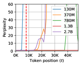
(a) Mamba-2 Series on the “newlines” prompt (only “\n” characters).

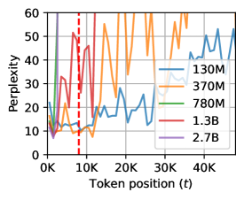
(b) Mamba-2 series on long documents from RedPajama.

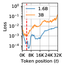
(c) RWKV-6 1.6B and 3B on the “newlines” prompt.

Figure 1: The perplexity of Mamba-2 and RWKV-6 as a function of token position on real and synthetic data. The red dotted line represents the models’ training lengths. They all fail to extrapolate.

Model checkpoints and source code are released at https://www.github.com/thunlp/stuffed-mamba.

2 Related Works

RNN-Based Language Models

There is a recent surge of interest in RNN-based language models, because, contrary to transformer-based ones, their per-token inference cost does not increase with the sequence length. Linear Attention (Katharopoulos et al., 2020) replaces the softmax attention in transformer-based models with kernel-based approximations that have equivalent recurrent formulations. Some notable recent RNNs include the RWKV series (Peng et al., 2023a; 2024), the Mamba series (Gu & Dao, 2023; Dao & Gu, 2024), Gated Linear Attention (Yang et al., 2023), among others (Zhang et al., 2024b; Yang et al., 2024; De et al., 2024; Arora et al., 2024; Orvieto et al., 2023; Sun et al., 2023). These models have shown strong capabilities in many language processing tasks, sometimes outperforming transformer-based models. However, as we will empirically show, some of these models fail to extrapolate much beyond their training length.

Some transformer-based models have adopted sliding window attention (Beltagy et al., 2020; Jiang et al., 2023), which essentially turns them into RNNs. However, these models have been shown to perform poorly in long-context tasks and fail to extrapolate to very long contexts (Zhang et al., 2024a).

Length Generalization

Most SOTA language models in the last few years have been based on the transformer (Vaswani et al., 2017) architecture. These models, when using certain variants of position encoding, can process arbitrarily long sequences. However, they exhibit severe performance drops on tokens beyond the training length (Zhao et al., 2024). To alleviate this shortcoming, many works have focused on modifying positional encoding (Peng et al., 2023b; Zhu et al., 2023; Ding et al., 2024; Jin et al., 2024), some achieving training-free length generalization to certain extents. Similarly in spirit, this study also explores some post-training modifications for enhancing RNN-based models’ length generalization capabilities.

Length Generalization of Mamba

Some concurrent works have explored extending Mamba’s context length by controlling the discretization term ($\Delta_{t}$ in Eq. 3) (Ben-Kish et al., 2024), such as dividing it by a constant to make it smaller. This essentially makes the memory decay factor ($\alpha_{t}$ in Eq. 4) closer to 1, which makes the state retain more contextual information. However, it also unnecessarily diminishes the inserted information on all tokens. Consequently, although it can mitigate SC, it results in poor performance in the passkey retrieval task (details in Appendix C).

3 Preliminary

Most experiments in this study focus on Mamba-2 (Dao & Gu, 2024) because it has shown strong capabilities on several tasks and has publicly available checkpoints of multiple sizes, allowing us to explore the relationship between state sizes and length limits. Moreover, it is more widely studied than other RNNs, making it easier to use existing works as a reference.

Mamba-2

The Mamba-2 architecture consists of a stack of $L$ Mamba-2 layers, each Mamba-2 layer consists of $H$ heads that are computed in parallel, and the output of a layer is the sum of the output of each head. Each head in each layer can be formulated as follows.

$$y_{t} =\text{Norm}(o_{t}\odot u_{t}W_{\text{gate}})W_{o}\in\mathbb{R}^{d}$$ (1)

$$o_{t} =C_{t}h_{t}+D\odot x_{t}\in\mathbb{R}^{P}$$ (2)

$$h_{t} =h_{t-1}\overline{A}_{t}+\overline{B}_{t}^{T}x_{t}\in\mathbb{R}^{N\times P}$$ (3)

where $t$ denotes the current time step, $u_{t},y_{t}\in\mathbb{R}^{d}$ are the input and output hidden representations of the $t$-th token, $\text{Norm}(\cdot)$ denotes the RMS normalization (Zhang & Sennrich, 2019), $D\in\mathbb{R}^{P}$, $W_{\text{gate}}\in\mathbb{R}^{d\times P}$, and $W_{o}\in\mathbb{R}^{P\times d}$ are trainable parameters, $\odot$ denotes element-wise product, and $d,N,P$ are hyperparameters, denoting the hidden dimensionality, state dimension, and head dimension, respectively. The other variables are parameterized as follows:

$$\overline{A}_{t} =\alpha_{t}I\in\mathbb{R}^{P\times P}$$ (4)

$$\overline{B}_{t} =\Delta_{t}B_{t}\in\mathbb{R}^{N}$$ (5)

$$\alpha_{t} =\exp(-\Delta_{t}\exp(A))\in\mathbb{R}$$ (6)

$$C_{t} =\sigma(\text{Conv}(u_{t}W_{C}))\in\mathbb{R}^{N}$$ (7)

$$B_{t} =\sigma(\text{Conv}(u_{t}W_{B}))\in\mathbb{R}^{N}$$ (8)

$$x_{t} =\sigma(\text{Conv}(u_{t}W_{x}))\in\mathbb{R}^{P}$$ (9)

$$\Delta_{t} =\text{Softplus}(u_{t}W_{\Delta}+b_{\Delta})\in\mathbb{R}$$ (10)

where $\left(W_{C},W_{B}\in\mathbb{R}^{d\times N},W_{x}\in\mathbb{R}^{d\times P},W_{\Delta}\in\mathbb{R}^{d\times 1},b_{\Delta},A\in\mathbb{R}\right)$ are trainable model parameters. $\text{Conv}(\cdot)$ denotes a channel-wise one-dimensional convolutional layer (more details in Appendix A.2). $\sigma$ denotes the SiLU function (Elfwing et al., 2017). Importantly, $h_{t}$ is called the hidden state or recurrent state, which is contextual memory that stores information from all tokens up to $t$. $\alpha_{t}$ is the decay multiplier that controls the strength of memory decay (i.e., forgetting). A more detailed formulation is given in Appendix A.

It is worth mentioning that since $\overline{A}_{t}$ is scalar-identity, the update rule can be seen as a variant of Gated Linear Attention (Yang et al., 2023) and is very similar to many existing RNNs such as RWKV (Peng et al., 2024) and RetNet (Sun et al., 2023). Thus, much of the experiments and insights may apply to other architectures. We leave such exhaustive ablation studies for future work.

4 State Collapse

We first examine state collapse (SC)—a phenomenon that causes RNN models to exhibit abnormal behaviors on inputs longer than those seen during training. We analyze the effects of SC on language modelings and the passkey retrieval task. Then we trace SC to the components of the state’s update rule and provide an explanation regarding training length overfitting. Finally, we propose three training-free mitigation methods by modifying the update rule and one method based on continual pre-training on longer sequences to avoid overfitting.

4.1 Length Generalization Failure

Language Modeling

Figure 1 shows the language modeling loss of Mamba-2 and RWKV-6 beyond their training lengths. For controllability and to synthesize prompts of arbitrary lengths, this loss is computed on a prompt consisting of only the “\n” characters, which we refer to as the “newlines” prompt. However, we emphasize that the same observation also exists when processing texts from the pre-training corpus. The result shows that both RNNs suffer great performance degradation when the context length is much longer than their training lengths, converging around the loss of random guessing.

Passkey Retrieval Evaluation

Language modeling may not reflect downstream capabilities, thus, we evaluate several strong RNNs on the passkey retrieval task (Mohtashami & Jaggi, 2023; Zhang et al., 2024a), a simple synthetic task where a model is prompted to recall a 5-digit passkey from a lengthy context. The hyperparameters and results of other RNNs can be found in Appendix B and D. The results for Mamba-2 are reported in Figure 2. We find that Mamba-2 models fail to generalize to sequences longer than the training length. For instance, Mamba-2, trained on 8K context windows, has near-perfect retrieval accuracy within 8K contexts (except for the smaller 130M checkpoint), but poor or even zero accuracy on sequences longer than 16K, regardless of model sizes.

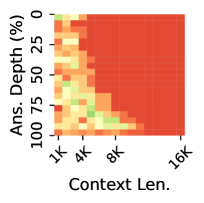
(a) 130M

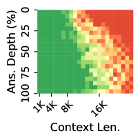
(b) 370M

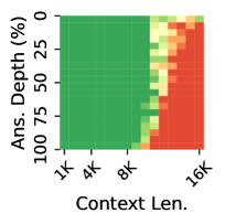
(c) 780M

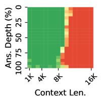
(d) 1.3B

Figure 2: The performance of Mamba-2 official checkpoints on the passkey retrieval task.

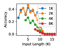
(a) 130M

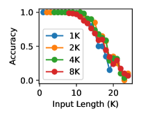
(b) 370M

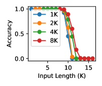
(c) 780M

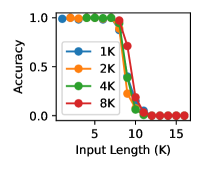
(d) 1.3B

Figure 3: The accuracy of Mamba-2 official checkpoints on the passkey retrieval task where the answer is in the last $n$ tokens, with $n$=1K, 2K, 4K, and 8K.

This behavior is unexpected because the update rule (Eq. 3) has a stable exponential memory decay (it converges to a constant value if the variables are fixed). Therefore, we expect that RNNs of such form should have a good retrieval accuracy on the last $k$ tokens, and tokens earlier than that are forgotten. This unexpected finding also implies that when processing contexts longer than the training length $T_{\text{train}}$, it is better to keep just the last $T_{\text{train}}$ tokens and discard everything else. However, this is not trivial in an online inference scenario because all token information is compressed into a single state.

4.2 What is the Cause of State Collapse?

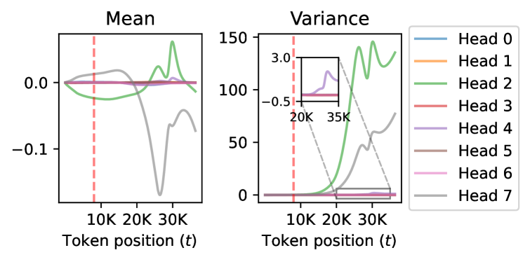
Figure 4: The mean and variance of the first 8 heads in the 38th layer of Mamba-2 370M. It exhibits a clear explosion when $t$ is greater than the training length. The red dotted line indicates the training length.

Figure 5: The distribution of the channels in a collapsing state (head 2 for the 38th layer) at two different time steps.

Since the recurrent state’s dimensionality does not change over time, the sharp change of behavior during state collapsing must be a result of a change in the state’s value. We inspect the statistics of the recurrent states of each layer in Mamba-2 370M and find that the mean and variance of some heads change sharply when the context length exceeds the training length, as shown in Figure 5. Appendix G includes a more detailed report on the statistics of each head. The state at $t=20K$ of one head with exploding variance is shown in Figure 5. From it, we discover that this variance explosion can be largely attributed to a few outlier channels, while most channels are relatively stable.

We emphasize that SC occurs largely independent of the prompt, occurring in both pre-training data samples and generated meaningless texts, even for prompts consisting of only whitespace characters (Figure 1 (a) and (b) shows SC on two different prompts). This means that the information inserted into the state does not cause its collapse.

To further attribute to the specific variables that cause SC, we inspect the values of $\Delta_{t}$, $B_{t}$, and $x_{t}$ on various heads with collapsing states. Figure 6 reports one example of the inspection, we can see that $x_{t}$ is relatively stable compared to the $\Delta_{t}$ and $B_{t}$, even though they are all functions of $u_{t}$. We also notice that $B_{t}$ explodes earlier than $\Delta_{t}$. Therefore, we conclude that the collapse is largely attributable to $B_{t}$. Further inspection reveals that the convolutional weights that generate $\Delta_{t}$ and $B_{t}$ (Eq. 8 and 10) are noticeably greater in variance than those for $x_{t}$ (Eq. 9). We leave a more in-depth attribution study for future work.

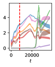
(a) $\Delta_{t}$. Each curve represents a head.

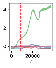
(b) $B_{t}$. Each curve represents a channel.

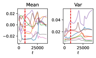
(c) The statistics of $x_{t}$ over time. Each curve represents a head.

Figure 6: The value of the components in the update rule ($\Delta_{t}$, $B_{t}$, and $x_{t}$) on some heads with SC in the 38th layer in Mamba-2 370M. The red dotted line indicates the training length.

4.2.1 State Collapse as a Result of State Overparameterization

Figure 7: The cumulative decay of the first token ($\alpha_{1:t}$) over time. Each line represents a head. The statistics are collected from the 38th layer of Mamba-2 370M.

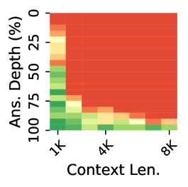
(a) 10B tokens.

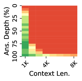
(b) 20B tokens.

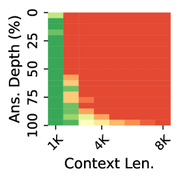
(c) 40B tokens.

Figure 8: The passkey retrieval results of intermediate checkpoints during the pre-training of Mamba-2 370M on 512 sequence length. SC only occurs in the model beyond a certain amount of training data.

Here, we present a high-level explanation for SC. We argue that SC arises from state overparameterization relative to the training length. In other words, the state capacity is excessively large for the training length, allowing the model to achieve strong language modeling performance without learning how to forget when the state is about to overflow. To support this argument, we formulate the hidden state as a weighted sum of previously inserted information:

$$h_{t}=\sum_{i=1}^{t}\alpha_{i:t}\overline{B}_{i}x_{i},\quad\alpha_{i:t}=\left(\prod_{j=i}^{t}\alpha_{j}\right)\in(0,1)$$ (11)

Therefore, $\alpha_{i:t}$ describes the memory strength about the $i$-th token at $t$ time step. Figure 8 shows the memory strength of the first token at different time steps, and we find that the exploded heads (heads 2, 4, and 7 in the 38th layer) have a strong inclination toward retaining all information within the training length, with a memory strength of over 0.8 at $t$=8K. This implies that the model has not learned to forget information (by producing a smaller decay $\alpha_{j}$) in a manner to avoid overflowing the state with too much information. Furthermore, we pre-train Mamba-2 from scratch with $T_{\text{train}}=512$ and evaluate the intermediate checkpoints on passkey retrieval, as reported in Figure 8. It shows that SC is only exhibited by checkpoints beyond a certain amount of training, which coincides with behaviors of overfitting—a result of overparameterization. One can also notice that the overfitted checkpoint outperforms earlier checkpoints on shorter sequences, which further strengthens the hypothesis that the model converges to less forgetting. Finally, as we will show in Section 4.3.2, for any given training length, there exists a state size where SC will be exhibited if and only if the model’s state size is greater.

4.3 How to Mitigate State Collapse?

Based on the analyses in the previous section, we propose several SC mitigation methods to make the model generalize better along the sequence length. In brief, we propose three training-free methods by modifying the update rule to avoid overflowing the state. Additionally, we directly train on longer sequences to encourage learning to smoothly forget the earliest information when the context is too long.

4.3.1 Training-Free Mitigation Methods

Method 1: Forget More and Remember Less

Since the variance of the state explodes during SC, we can reduce this by increasing the amount of state decay (i.e., forget more) or reducing the amount of inserted information (i.e., remember less). Based on the analysis in Section 4.2, we choose to intervene in the components $B_{t}$ and $\alpha_{t}$, which control the insertion strength and memory decay strength, respectively. Existing works have experimented with modifying $\Delta_{t}$, but it controls both the insertion and decay strength, making it hard to analyze and control.

Method 2: State Normalization

The main idea is to normalize the state after each update to ensure that the state’s norm is always below a threshold $p\in\mathbb{R}$. Specifically, we decay the state $h_{t}$ at each time step to ensure that $\|h_{t}\|\leq p$. Thus, we get the following update rule.

$$\hat{h}_{t} =h_{t-1}\overline{A}_{t}+\overline{B}^{T}x_{t}$$ (12)

$$h_{t} =\begin{cases}\hat{h}_{t}p/\|\hat{h}_{t}\|&\text{ if }\|\hat{h}_{t}\|>p\\ \hat{h}_{t}&\text{ if }\|\hat{h}_{t}\|\leq p\\ \end{cases}$$ (13)

It is worth mentioning that this converts the model into a non-linear RNN and cannot be parallelized in the same manner as the original model, making it much slower at pre-filling.

Method 3: Sliding Window by State Difference

We can utilize the fact that the state $h_{t}$ can be written as a weighted sum (Eq. 11) to simulate a sliding window mechanism without re-processing from the start of the window at every step. Let $w\in\mathbb{N}$ denote the window size and $h_{t}^{(r)}\in\mathbb{R}^{N\times P}$ denote the hidden state when applying the model on the last $w$ tokens at time step $t$. We can then compute $h_{t}^{(r)}$ exactly as the difference between two states:

$$h_{t}^{(r)}=\sum_{i=t-r+1}^{t}\alpha_{i:t}\hat{R}_{i}=\sum_{i=1}^{t}\alpha_{i:t}\overline{B}_{i}^{T}x_{i}-\alpha_{t-r+1:t}\sum_{i=1}^{t-r}\alpha_{i:t-r}\overline{B}_{i}^{T}x_{i}=h_{t}-\alpha_{t-r+1:t}h_{t-r}$$ (14)

During streaming generation, we only have to maintain $(h_{t-1},h_{t-r},\alpha_{t-r+1:t})$, and advance each of them in parallel. However, directly computing $\alpha_{t:t-r}$ may suffer from instability due to floating-point imprecision. Therefore, we maintain $\Delta_{t-r:t}=\sum_{i=t-r}^{t}\Delta_{t}$ instead, and re-compute $\alpha_{t-r:t}=\exp\left(-\Delta_{t-r:t}\exp(A)\right)$ at every step, which incurs minimal computational cost.

This method applies to all RNNs that can be written as a weighted sum, which includes RWKV 5 and 6, RetNet, GLA, etc. It doubles the computation and memory cost for generation, but we believe that it is an acceptable trade-off because RNNs have a very low generation cost compared to transformer-based models and the context processing cost is unchanged.

4.3.2 Training on Longer Sequences

Based on the hypothesis that SC is caused by state overparameterization (described in Section 4.2.1), we can simply train on lengths that exceed the state capacity, which we conduct in this section.

Data Engineering

To ensure that the data contains as much long-term structure as possible, we filter out sequences with less than 4K tokens. Buckman & Gelada (2024) have shown that this is critical for training effective long-context models. Although we train on sequences longer than 4K tokens, we do not use a higher length threshold because the above threshold already removes about 97.6% of the data in the original corpus. To train on longer sequences, we simply concatenate sequences and delimit them with a special EOS (End-of-Sequence) token.

Truncated Backpropagation Through Time

In the vanilla Mamba-2, the states are initialized to zeros for each data sample. Instead, we initialize the states as the final state of the previous sequence. This is equivalent to concatenating multiple sequences, but stopping the backpropagation of gradients at certain intervals. This technique has been shown to help extend the context length of RNNs (Yang et al., 2023) and alleviate the memory cost of caching activations for computing gradients. Based on Yang et al. (2023) and our preliminary tests, we use concatenate 12 sequences with this technique by default.

5 State Capacity

Based on the discussion in Section 4.2.1, SC occurs if and only if the training length contains less information than the state capacity. Thus, we can indirectly estimate state capacity by sweeping different training lengths for different state sizes, and observing when the state does not collapse. In this section, we empirically investigate the relationship between state capacity and state size.

Specifically, we conduct the same training as in Section 4.3.2. To determine whether a state has collapsed, we feed the “newlines” prompt with 1M tokens to the model, and define collapse as the point where perplexity is more than 2x the maximum perplexity in its training length. We train multiple Mamba-2 with different state sizes and training lengths, and we regard the minimum training length at which SC does not occur as the state capacity.

5.1 State Capacity in Passkey Retrieval

The language modeling performance may not reflect the downstream capabilities well (Fu et al., 2024). Therefore, we also search for the state capacity on the passkey retrieval task. Similar to the previous section, we train with different lengths for different state sizes and identify the maximum context length where the model has an accuracy over 95%, which we regard as the state capacity in passkey retrieval. In this task, the noisy context is repetitive, thus, the amount of contextual information is largely independent of the context length, therefore, the capacity should grow roughly exponentially with the state size.

It is worth emphasizing that, if we train Mamba-2 on passkey retrieval data, the model can theoretically handle infinitely long contexts by ignoring all irrelevant tokens. Here, the model is only trained with the next token prediction objective, which means the model will not ignore the irrelevant context, and the ability to retain information for extended time emerges from language modeling.

6 Experiments

We briefly describe the experimental details for length extrapolation experiments.

Data

We start from RedPajama-V2 (Computer, 2023), an open dataset with 30T tokens extracted from CommonCrawl, and we perform deduplication to ensure data quality. During evaluation, we sample documents longer than 16K tokens and concatenate them if it is not long enough.

Models

We experiment with seven model configurations with different state sizes to find the relationship between state capacity and size. For each of them, we perform an extensive search with training lengths up to 256K tokens. To save cost, we continue pre-train from three official checkpoints of Mamba-2 of size 130M, 370M, and 780M. They are all trained on 8K sequences. The other three model configurations (36M, 47M, and 85M) are trained from scratch. The detailed configurations are given in Appendix F.1.

Hyperparameters

We use the WSD (Hu et al., 2024) with 10% decay steps. This scheduler is chosen because it is competitive with the commonly used cosine scheduler while allowing simple resumption from intermediate checkpoints, saving large amounts of computational resources. We report the result of the best checkpoint selection by validation on passkey retrieval. More hyperparameters are reported in the Appendix F.

7 Results

7.1 Training-Free Length Generalization

Figure 9 reports the result of the training-free length generalization methods on Mamba-2 780M. We can see that while LongMamba can greatly improve the length generalizability of the model by more than 3x, it causes noticeably greater perplexity on shorter sequences and still inevitably exhibits SC. All our methods successfully suppress SC, allowing the model to generalize to more than 64K tokens, although State Normalization greatly underperforms other methods on shorter sequences. One explanation for this underperformance is that normalizing collapsing states changes the ratio of norms between heads, and this disrupts the learned mechanisms.

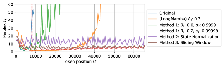
Figure 9: Result of training-free length generalization methods described in Section 4.3.1. Perplexity is computed on long documents from RedPajama (Computer, 2023). The red dotted line represents the training length.

7.2 Length Generalization by Training on Longer Sequences

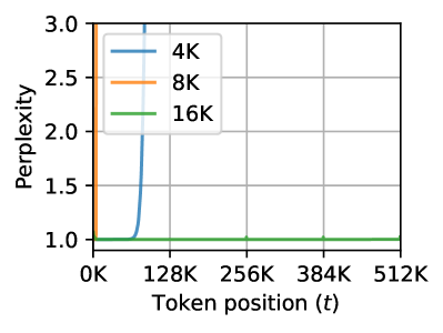
(a) 130M.

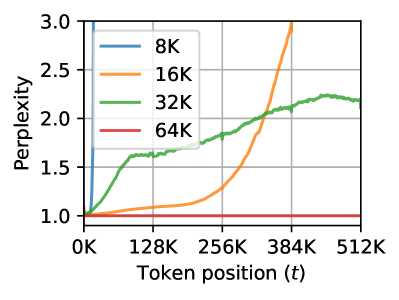
(b) 370M.

Figure 10: The perplexity as a function of token position for Mamba-2 130M on the “newlines” prompt with three different training lengths.

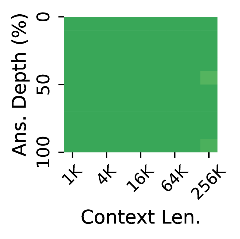
Figure 11: Passkey retrieval Performance of the best checkpoint of Mamba-2 370M. The x-axis is in the log scale.

In Figure 11, we plot the language modeling perplexity as a function of token position for Mamba-2 130M and 370M with different training lengths. We can see that for each model size, there is a training length threshold, beyond which the model has much better length extrapolation, which supports our arguments discussed in Section 4.3.2.

7.3 State Capacity as a Function of State Size

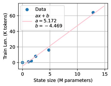
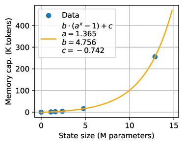
Figure 12: The left figure shows the training length beyond which the model does not exhibit SC. The right figure shows the memory capacity on passkey retrieval as a function of state size.

Figure 12 shows the state capacity of Mamba-2 on language modeling and passkey retrieval. The rightmost data point in both plots corresponds to Mamba-2 370M. We have confirmed that 780M also exhibits SC at training lengths below 128K, but do not have enough resources to train the model beyond this length. The results establish a linear relationship $T_{\text{train}}=5.172\cdot S-4.469$ between the length $T_{\text{train}}$ at which SC stops occurring and the state size $S$.

The second plot of Figure 12 shows that the capacity of Mamba-2 on passkey retrieval is exponential concerning the state size. This is because the amount of information in the context does not increase with its length. In other words, we are storing a constant amount of information while the number of combinations of the state grows exponentially with the number of elements. Figure 11 shows the best checkpoint of Mamba-2 370M on passkey retrieval. The result is very promising because, to the best of our knowledge, no previous models with less than 1B model parameters have near-perfect accuracy at 128K tokens in this task.

8 Conclusion

This paper discovers and presents the first systemic study on state collapse (SC), a phenomenon in RNNs that causes length generalization failure. With an inspection of the activations and controlled experiments on Mamba-2, we conclude that this phenomenon is caused by an overparameterized state with excessive state capacity. Based on the analyses, we have proposed three training-free methods for mitigating SC up to 1M tokens. Then, we show that SC can be mitigated by training on context lengths that exceed the state capacity. With this insight, we empirically estimate the state capacity of Mamba-2 on language modeling and the passkey retrieval task. With some simple data engineering and state initialization tricks, we achieve much better performance with Mamba-2 on the passkey retrieval task than existing models. Our results indicate that Mamba-2 not only is highly efficient in handling long sequences but also has great performance potential.

Limitations

All models studied in this work can be seen as a specific case of linear attention models, whose recurrent state is decayed by an element-wise or scalar gate (they can be viewed as variants of Gated Linear Attention (Yang et al., 2023)). We have chosen to study these models because of their strong capabilities, yet, some conclusions may not be directly transferred to other variants of RNNs.

Our continued pre-training approach for extending the context length of RNNs is rather expensive, some of the models require training with up to 50B tokens, which is 1/6 of their pre-training amount of data. Also, to ensure simplicity, controllability, and generality, we have not used more advanced techniques for training long-context models, such as upsampling longer data samples, better data order or format, using data with more long-distance dependencies, etc.

The passkey retrieval task that we used extensively in this study is very simple. Hence, high accuracy on this task may not reflect the capabilities of the model on real-world long-context tasks, because that requires more advanced capabilities such as high-resolution retrieval, reasoning, state-tracking, etc. The result is nonetheless promising because it indicates that the model can recall the correct information and further capabilities may be achieved by building on the recalled information.

SC is somewhat prompt-dependent. While we found that for models with greatly overparameterized states, SC is highly consistent across different prompts, certain models with less overparameterization may exhibit SC on some prompts while successfully extrapolating indefinitely on others. Attributing SC to specific features of the prompt is a promising future research direction.

Appendix A Mamba-2 Architecture

For completeness, we give a more detailed formulation of the Mamba-2 architecture here, although we recommend the readers refer to the original paper (Dao & Gu, 2024) or a detailed blog post by the authors. The model accepts a sequence of $T$ token IDs as input $\mathbf{I}=[i_{1},\cdots,i_{T}]\in\mathbb{R}^{T},i_{t}\in\{1,2,\cdots,V\}$, where $V$ denotes the vocabulary size. It performs next token prediction by predicting the probability distribution over the vocabulary as each time step, denoted as $P\in\mathbb{R}^{T\times V}$. The model can be formulated as follows.

$$\mathbf{U}^{(0)} =\text{Embed}_{\text{in}}(\mathbf{I})\in\mathbb{R}^{T\times d}$$

$$\mathbf{U}^{(l)} =\text{Mamba}^{(l)}\left(\text{Norm}\left[\mathbf{U}^{(l-1)}\right]\right)\in R^{T\times d}$$

$$\mathbf{P} =\text{Embed}_{\text{out}}\left(\text{Norm}\left[\mathbf{U}^{(L)}\right]\right)\in\mathbb{R}^{T\times V}$$

where $L$ denotes the number of layers, $l\in\{1,\cdots,L\}$ denotes the layer index, $\mathbf{U}^{(l)}\in\mathbb{R}^{T\times d}$ represents the input of the $l$-th layer, $\mathbf{U}^{(0)}$ represents the input of the first layer. $\text{Mamba}^{(l)}(\cdot)$ denotes the $l$-th Mamba layer, $\text{Embed}_{\text{in}}(\cdot)$ and $\text{Embed}_{\text{out}}(\cdot)$ denote the input and output embedding layers, and $\text{Norm}(\cdot)$ denotes RMS normalization (Zhang & Sennrich, 2019). $d$ denotes the number of dimensions of each token embedding. Similar to many other models, Mamba-2 ties the weight of the input and output embedding layers.

Each Mamba layer consists of $H$ “heads” that are computed in parallel. The result of which is summed together. The $t$-th token ($t\in\{1,\cdots,T\}$) in a head is computed as follows.

$$y_{t} =\text{Norm}(o_{t}\odot u_{t}W_{\text{gate}})W_{o}\in\mathbb{R}^{d}$$

$$o_{t} =C_{t}h_{t}+D\odot x_{t}\in\mathbb{R}^{P}$$

$$h_{t} =h_{t-1}\exp(-\Delta_{t}\exp(A))+\Delta_{t}B_{t}^{T}x_{t}\in\mathbb{R}^{N\times P}$$

$$C_{t} =\sigma(\text{Conv}(u_{t}W_{C}))\in\mathbb{R}^{N}$$

$$B_{t} =\sigma(\text{Conv}(u_{t}W_{B}))\in\mathbb{R}^{N}$$

$$x_{t} =\sigma(\text{Conv}(u_{t}W_{x}))\in\mathbb{R}^{P}$$

$$\Delta_{t} =\text{Softplus}(u_{t}W_{\Delta}+b_{\Delta})\in\mathbb{R}$$

$u_{t}$ denotes the $t$-th input representation. In other words, for the $l$-th layer, we have $\mathbf{U}^{(l)}=\left[u_{1}^{(l)},\cdots,u_{T}^{(l)}\right]$, $\mathbf{U}^{(l+1)}=\left[y_{1}^{(l)},\cdots,y_{T}^{(l)}\right]$, and $u_{t}^{(l+1)}=y_{t}^{(l)}$. $\text{Conv}(\cdot)$ denotes a channel-wise one-dimensional convolutional layer with a kernel size of 4, and $\sigma$ denotes the SiLU activation function (Elfwing et al., 2017). All vectors are row vectors, and the result of a matrix multiplied by a scalar is the matrix with each element multiplied by that scalar.

$\left(W_{\text{gate}},W_{x}\in\mathbb{R}^{d\times P},W_{o}\in\mathbb{R}^{P\times d},W_{C},W_{B}\in\mathbb{R}^{d\times N},W_{\Delta}\in\mathbb{R}^{d\times 1},b_{\Delta},A\in\mathbb{R}\right)$ are trainable parameters of the layer, and $P,N$ are hyperparameters. The authors call $P$ the head dimension and $N$ the state size. In practice, the weights of $W_{B},W_{C}$ are shared among different heads.

A.1 State Size

The authors of Mamba-2 always set $P=64$, $N=128$, and $H=2d/P$. Thus, the state size of each Mamba-2 layer is $HPN=2dN=256d$. In transformer-based models, when using multi-headed attention, usually, the product of the head count $H$ and head dimension $P$ equals the hidden dimension $d$. Therefore, the KV cache of a transformer-based model is $2Td$, which means that when using the same hidden dimension, the state of a Mamba-2 layer is equal in size to a KV cache of 128 tokens.

Compared to many other recurrent models (e.g., the RWKV series (Peng et al., 2023a; 2024), GLA (Yang et al., 2023), and RetNet (Sun et al., 2023)), Mamba-2 does not have a state-less feed-forward network and has considerably more heads in each layer, making the state size much larger than other recurrent models. Compared to Mamba-1 (Gu & Dao, 2023), Mamba-1 uses $N=16$, which means that the state size in Mamba-2 is 8 times larger than the state in a Mamba-1 model of roughly the model parameter count. Figure 13 shows the relationship between state size and model size of the RNN models in this study.

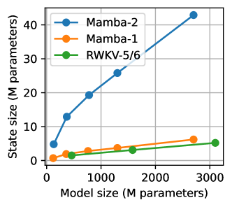
Figure 13: The relationship between state size and model size of various RNN models considered in this paper.

A.2 Short Convolution

The $\text{Conv}(\cdot)$ function in Mamba-2 is a one-dimensional convolutional layer applied to each channel separately. For $i$-th channel, it can be formulated as follows.

$$y_{t,i}=\sum_{j=1}^{k}w_{j,i}x_{t-j,i}\in\mathbb{R},\quad i=1,\cdots,n_{c}$$

$k$ denotes the kernel size (set to 4 by default). $i$ denotes the channel index, $n_{c}$ denotes the number of channels. $y_{t,i}\in\mathbb{R}$ denotes the $i$-th channel of the output vector at $t$-th time step. $x_{t,i}$ represents the $i$-th channel of the input vector at $t$-th time step. $w_{j,i}\in\mathbb{R}$ denotes the $j$-th value in the convolutional kernel for channel $i$.

This model component accepts the last 4 token embeddings at the input. Therefore, it also has a state that contains information about the context, which we refer to as the convolutional state. To be concrete, due to information propagation through the layers, the short convolutional layer is a function of the last $4L$ tokens. For the 370M model size, this length is $4\times 48=192$. Therefore, we can reasonably assume that this component contains much less contextual information relative to the recurrent state $h_{t}$. Thus, we have largely ignored this state in various discussions in this paper. However, we have also reported the distribution of the input to this short convolutional layer over time in Figure 18, for reference. As we can see, the convolutional state is relatively stable over time.

Appendix B Passkey Retrieval Inference Parameters

Throughout the whole paper, we use greedy decoding, not just for reproducibility, but also because our preliminary results show that other decoding parameters give noticeably worse performance on passkey retrieval.

We use 32-bit floating point precision for both model parameters and activations during inference, to ensure that precision errors do not introduce noise to the result. We have conducted some preliminary evaluations with BF16 and FP16 and found that there are no noticeable differences with using FP16, but computing some activations, especially the $\Delta_{t}$ and $\alpha_{t}$ with BF16 introduces an error around 1e-3. However, the explosion of channels in the states is consistently observed despite this precision error.

B.1 Passkey Retrieval Prompt

The prompt that we use for the passkey retrieval task is as follows, using 34847 as the passkey for example, which is adapted from existing works (Zhang et al., 2024a). We also evaluate with slight variations to the template in preliminary experiments but do not observe considerable differences in the results.

There is important info hidden inside a lot of irrelevant text. Find it and memorize it.
The grass is green. The sky is blue. The sun is yellow. Here we go. There and back again.
...
The grass is green. The sky is blue. The sun is yellow. Here we go. There and back again.
The passkey is 34847. Remember it. 34847 is the passkey.
The grass is green. The sky is blue. The sun is yellow. Here we go. There and back again.
...
The grass is green. The sky is blue. The sun is yellow. Here we go. There and back again.
What is the passkey? The passkey is

We sweep different context lengths $T\in\{1K,2K,...,256K\}$, and for each length $T$, we generate $n$ prompts with evenly distributed needle positions, i.e., the $i$-th needle ($i\in\{0,\cdots,n-1\}$) of a sample is inserted at position $T\times i/n-1$, from the beginning.

Appendix C Mamba-2 with Modified $\Delta_{t}$ on passkey retrieval

Ben-Kish et al. (2024) and GitHub user jzhang28 propose to improve Mamba’s length generalization by reducing the value of $\Delta_{t}$. Ben-Kish et al. (2024) propose a heuristic method for identifying which head to modify and how to modify $\Delta_{t}$. However, their method requires task-dependent tweaking, so we do not consider comparing against it. jzhang28 propose to simply multiply $\Delta_{t}$ by a constant (they used 0.5). We apply this method and sweep different $\Delta_{t}$ for the best passkey retrieval performance, but they all result in worse performance than the original model across all context lengths.

Appendix D Passkey Retrieval Evaluation with Other Architectures

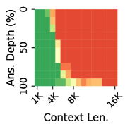
(a) 1.5B

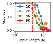
(b) 1.5B

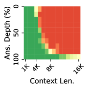
(c) 3B

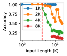
(d) 3B

Figure 14: The performance of RWKV-5 official checkpoints on the passkey retrieval task. Each curve in (b) and (d) represents the accuracy of retrieving the needle when it is within the last $r$ tokens, with $r\in\{1K,2K,4K,8K\}$.

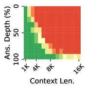
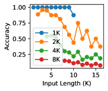
Figure 15: RWKV-6 1.6B result on the passkey retrieval task. The left plot shows the retrieval accuracy of the needle when it appears in the last $r=\{1K,2K,4K,8K\}$ tokens.

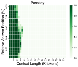
(a) 790M

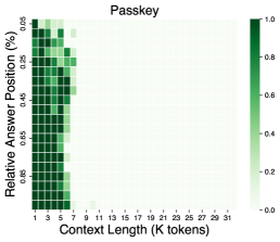
(b) 1.4B

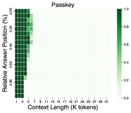
(c) 2.8B

Figure 16: The performance of Mamba-1 official checkpoints on the Passkey task. We can see a clear exhibition of state collapse, similar to Mamba-2.

Here, we also evaluate RWKV-5, RWKV-6, and Mamba-1 (some popular and strong RNNs) on the passkey retrieval task. The result is reported in Figure 14, 15 and 16. We can see that SC is observed in Mamba-1, but it is less severe for RWKV-5 and RWKV-6. We hypothesize that this difference is a result of architectural differences and that the state size is smaller in RWKV-5 and RWKV-6.

Appendix E Pre-Trained Checkpoints

The pre-trained checkpoints used in our experiments are given in Table 1.

Model	Checkpoint URLs
RWKV-5	https://huggingface.co/RWKV/rwkv-5-world-all-pth
RWKV-6	https://huggingface.co/RWKV/v6-Finch-1B6-HF https://huggingface.co/RWKV/v6-Finch-3B-HF
Mamba-1	https://huggingface.co/state-spaces/mamba-130m https://huggingface.co/state-spaces/mamba-370m https://huggingface.co/state-spaces/mamba-790m https://huggingface.co/state-spaces/mamba-1.4b https://huggingface.co/state-spaces/mamba-2.8b
Mamba-2	https://huggingface.co/state-spaces/mamba2-130m https://huggingface.co/state-spaces/mamba2-370m https://huggingface.co/state-spaces/mamba2-780m https://huggingface.co/state-spaces/mamba2-1.3b https://huggingface.co/state-spaces/mamba2-2.7b

Table 1: The pre-trained checkpoints used in our experiments.

Appendix F Length Extrapolation Training Details

We perform a hyperparameter search on learning rates, sweeping $\{1\mathrm{e}-5,2\mathrm{e}-5,5\mathrm{e}-5,1\mathrm{e}-4,2\mathrm{e}-4,5\mathrm{e}-4,\mathrm{1e-3}\}$, selecting the best performing one by validation on passkey retrieval. Regarding the WSD scheduler, it warms up linearly for 1000 steps and decays linearly with 50K steps. This setup is inspired by the authors of WSD (Hu et al., 2024).

Other hyperparameters are kept as similar to the original papers for Mamba-2 as possible. That means we use 0.5M tokens per batch, because we found this to give more stable results for continual pre-training instead of the 1M batch size from the original paper. Training is done mainly in BF16, with some activations in FP32 (in the same manner as the official implementation). The optimizer is AdamW, with a 0.1 weight decay. Moreover, we use 1.0 gradient clipping.

All experiments are run on A800 80G, some are run with multiple nodes, and others with multiple GPUs on a single node.

F.1 Model Configurations

For the models smaller than the 130M official checkpoint, we pre-train from scratch using the configurations reported in Table 2. We try to follow the same depth-to-width ratio found in the official checkpoints, although the ratio is not entirely consistent in those checkpoints. Hyperparameters not mentioned are kept the same as the 130M checkpoint.

Model size	State size	# Layers	Hidden dim.	# heads
Official checkpoints
780M	19.3M	48	1536	48
370M	12.9M	48	1024	32
130M	4.8M	24	768	24
Our checkpoints trained from scratch
84.6M	2.4M	12	768	24
47.0M	1.6M	12	512	16
36.4M	0.8M	6	512	16

Table 2: The configurations of the models used in finding the passkey retrieval memory capacity as a function of the state size.

Appendix G State Statistics over Context Length

Here, we provide a more detailed result on the inspection of SC over time.

G.1 The “newlines” Prompt

In this paper, we collect the statistics of the state computed on a “newlines” prompt, a prompt where every token is the newline token, as shown below.

\n\n\n\n\n\n\n\n\n\n\n\n\n\n\n\n\n\n...

However, we again emphasize that SC is observed on prompts extracted from the pre-training corpus, the passkey retrieval task, or other randomly generated sequences. We have chosen the “newlines” prompt because the samples from the pre-training corpus are too short, and this prompt produces the most consistent and smooth layer statistics.

Figure 17 shows the hidden state of the recurrent mechanism described in Eq. 3. Additionally, $B_{t}$, $C_{t}$, and $x_{t}$ in Mamba-2 are generated with a short channel-wise convolutional layer with a kernel size of 4:

$$B_{t}=\sigma(\text{Conv}[u_{t}W_{B}])$$

$$C_{t}=\sigma(\text{Conv}[u_{t}W_{C}])$$

$$x_{t}=\sigma(\text{Conv}[u_{t}W_{x}])$$

where $\sigma$ is the SiLU activation function. This function is also stateful because it operates on the last 4 tokens, therefore, we also collect the statistics of this convolutional state and report them in Figure 18. As we can see, the convolutional states are much more stable compared to the recurrent states. This is because only the last 4 tokens contribute to this state which avoids the explosion as a result of cumulative sum.

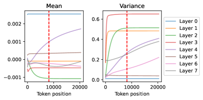
(a) Layer 0-7

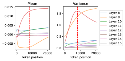
(b) Layer 8-15

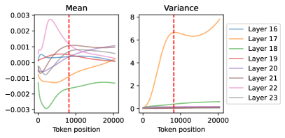
(c) Layer 16-23

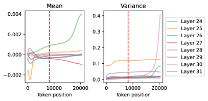
(d) Layer 23-31

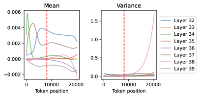
(e) Layer 32-39

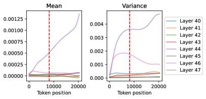
(f) Layer 40-48

Figure 17: The mean and variance of the hidden state of each layer of Mamba-2 370M, computed on the “newlines” prompt.

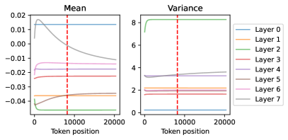
(a) Layer 0-7

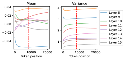
(b) Layer 8-15

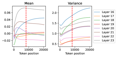
(c) Layer 16-23

(d) Layer 23-31

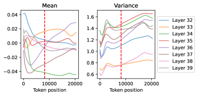
(e) Layer 32-39

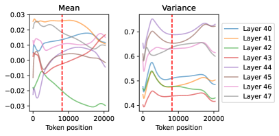
(f) Layer 40-48

Figure 18: The mean and variance of the convolutional states (the representation of the last four tokens) of each layer in Mamba-2 370M, computed on the “newlines” prompt.

References

- Achiam et al. (2023) Josh Achiam, Steven Adler, Sandhini Agarwal, Lama Ahmad, Ilge Akkaya, Florencia Leoni Aleman, Diogo Almeida, Janko Altenschmidt, Sam Altman, Shyamal Anadkat, et al. Gpt-4 technical report. arXiv preprint arXiv:2303.08774, 2023.
- Arora et al. (2024) Simran Arora, Sabri Eyuboglu, Michael Zhang, Aman Timalsina, Silas Alberti, Dylan Zinsley, James Zou, Atri Rudra, and Christopher Re. Simple linear attention language models balance the recall-throughput tradeoff. In Workshop on Efficient Systems for Foundation Models II @ ICML2024, volume abs/2402.18668, 2024.
- Beltagy et al. (2020) Iz Beltagy, Matthew E Peters, and Arman Cohan. Longformer: The long-document transformer. arXiv preprint arXiv:2004.05150, 2020.
- Ben-Kish et al. (2024) Assaf Ben-Kish, Itamar Zimerman, Shady Abu-Hussein, Nadav Cohen, Amir Globerson, Lior Wolf, and Raja Giryes. Decimamba: Exploring the length extrapolation potential of mamba, 2024.
- Bengio et al. (1994) Yoshua Bengio, Patrice Simard, and Palo Frasconi. Learning long-term dependencies with gradient descent is difficult. IEEE transactions on neural networks, 5(2):157–166, 1994.
- Brown et al. (2020) Tom B. Brown, Benjamin Mann, Nick Ryder, Melanie Subbiah, Jared Kaplan, Prafulla Dhariwal, Arvind Neelakantan, Pranav Shyam, Girish Sastry, Amanda Askell, Sandhini Agarwal, Ariel Herbert-Voss, Gretchen Krueger, Tom Henighan, Rewon Child, Aditya Ramesh, Daniel M. Ziegler, Jeffrey Wu, Clemens Winter, Christopher Hesse, Mark Chen, Eric Sigler, Mateusz Litwin, Scott Gray, Benjamin Chess, Jack Clark, Christopher Berner, Sam McCandlish, Alec Radford, Ilya Sutskever, and Dario Amodei. Language models are few-shot learners, 2020. URL https://arxiv.org/abs/2005.14165.
- Buckman & Gelada (2024) Jacob Buckman and Carles Gelada. Compute-optimal Context Size, 2024.
- Computer (2023) Together Computer. Redpajama: an open dataset for training large language models, October 2023. URL https://github.com/togethercomputer/RedPajama-Data.
- Dao & Gu (2024) Tri Dao and Albert Gu. Transformers are ssms: Generalized models and efficient algorithms through structured state space duality. arXiv preprint arXiv:2405.21060, 2024.
- De et al. (2024) Soham De, Samuel L. Smith, Anushan Fernando, Aleksandar Botev, George-Cristian Muraru, Albert Gu, Ruba Haroun, Leonard Berrada, Yutian Chen, Srivatsan Srinivasan, Guillaume Desjardins, Arnaud Doucet, David Budden, Yee Whye Teh, Razvan Pascanu, Nando de Freitas, and Caglar Gulcehre. Griffin: Mixing Gated Linear Recurrences with Local Attention for Efficient Language Models. arXiv, abs/2402.19427, 2024.
- Ding et al. (2024) Yiran Ding, Li Lyna Zhang, Chengruidong Zhang, Yuanyuan Xu, Ning Shang, Jiahang Xu, Fan Yang, and Mao Yang. Longrope: Extending llm context window beyond 2 million tokens. arXiv preprint arXiv:2402.13753, 2024.
- Dubey et al. (2024) Abhimanyu Dubey, Abhinav Jauhri, Abhinav Pandey, Abhishek Kadian, Ahmad Al-Dahle, Aiesha Letman, Akhil Mathur, Alan Schelten, Amy Yang, Angela Fan, et al. The llama 3 herd of models. arXiv preprint arXiv:2407.21783, 2024.
- Elfwing et al. (2017) Stefan Elfwing, Eiji Uchibe, and Kenji Doya. Sigmoid-weighted linear units for neural network function approximation in reinforcement learning, 2017. URL https://arxiv.org/abs/1702.03118.
- Fu et al. (2024) Yao Fu, Rameswar Panda, Xinyao Niu, Xiang Yue, Hannaneh Hajishirzi, Yoon Kim, and Hao Peng. Data engineering for scaling language models to 128k context, 2024. URL https://arxiv.org/abs/2402.10171.
- GLM et al. (2024) Team GLM, Aohan Zeng, Bin Xu, Bowen Wang, Chenhui Zhang, Da Yin, Diego Rojas, Guanyu Feng, Hanlin Zhao, Hanyu Lai, Hao Yu, Hongning Wang, Jiadai Sun, Jiajie Zhang, Jiale Cheng, Jiayi Gui, Jie Tang, Jing Zhang, Juanzi Li, Lei Zhao, Lindong Wu, Lucen Zhong, Mingdao Liu, Minlie Huang, Peng Zhang, Qinkai Zheng, Rui Lu, Shuaiqi Duan, Shudan Zhang, Shulin Cao, Shuxun Yang, Weng Lam Tam, Wenyi Zhao, Xiao Liu, Xiao Xia, Xiaohan Zhang, Xiaotao Gu, Xin Lv, Xinghan Liu, Xinyi Liu, Xinyue Yang, Xixuan Song, Xunkai Zhang, Yifan An, Yifan Xu, Yilin Niu, Yuantao Yang, Yueyan Li, Yushi Bai, Yuxiao Dong, Zehan Qi, Zhaoyu Wang, Zhen Yang, Zhengxiao Du, Zhenyu Hou, and Zihan Wang. Chatglm: A family of large language models from glm-130b to glm-4 all tools, 2024.
- Gu & Dao (2023) Albert Gu and Tri Dao. Mamba: Linear-time sequence modeling with selective state spaces. ArXiv, abs/2312.00752, 2023. URL https://api.semanticscholar.org/CorpusID:265551773.
- Hu et al. (2024) Shengding Hu, Yuge Tu, Xu Han, Chaoqun He, Ganqu Cui, Xiang Long, Zhi Zheng, Yewei Fang, Yuxiang Huang, Weilin Zhao, et al. Minicpm: Unveiling the potential of small language models with scalable training strategies. arXiv preprint arXiv:2404.06395, 2024.
- Jiang et al. (2023) Albert Q Jiang, Alexandre Sablayrolles, Arthur Mensch, Chris Bamford, Devendra Singh Chaplot, Diego de las Casas, Florian Bressand, Gianna Lengyel, Guillaume Lample, Lucile Saulnier, et al. Mistral 7b. arXiv preprint arXiv:2310.06825, 2023.
- Jin et al. (2024) Hongye Jin, Xiaotian Han, Jingfeng Yang, Zhimeng Jiang, Zirui Liu, Chia-Yuan Chang, Huiyuan Chen, and Xia Hu. Llm maybe longlm: Self-extend llm context window without tuning. arXiv preprint arXiv:2401.01325, 2024.
- Katharopoulos et al. (2020) Angelos Katharopoulos, Apoorv Vyas, Nikolaos Pappas, and François Fleuret. Transformers are rnns: Fast autoregressive transformers with linear attention. In International conference on machine learning, pp. 5156–5165. PMLR, 2020.
- Mohtashami & Jaggi (2023) Amirkeivan Mohtashami and Martin Jaggi. Landmark attention: Random-access infinite context length for transformers. In Workshop on Efficient Systems for Foundation Models@ ICML2023, 2023.
- Orvieto et al. (2023) Antonio Orvieto, Samuel L Smith, Albert Gu, Anushan Fernando, Caglar Gulcehre, Razvan Pascanu, and Soham De. Resurrecting recurrent neural networks for long sequences, 2023. URL https://arxiv.org/abs/2303.06349.
- Peng et al. (2023a) Bo Peng, Eric Alcaide, Quentin G. Anthony, Alon Albalak, Samuel Arcadinho, Stella Biderman, Huanqi Cao, Xin Cheng, Michael Chung, Matteo Grella, G Kranthikiran, Xuming He, Haowen Hou, Przemyslaw Kazienko, Jan Kocoń, Jiaming Kong, Bartlomiej Koptyra, Hayden Lau, Krishna Sri Ipsit Mantri, Ferdinand Mom, Atsushi Saito, Xiangru Tang, Bolun Wang, Johan Sokrates Wind, Stansilaw Wozniak, Ruichong Zhang, Zhenyuan Zhang, Qihang Zhao, Peng Zhou, Jian Zhu, and Rui Zhu. Rwkv: Reinventing rnns for the transformer era. In Conference on Empirical Methods in Natural Language Processing, 2023a. URL https://api.semanticscholar.org/CorpusID:258832459.
- Peng et al. (2024) Bo Peng, Daniel Goldstein, Quentin Anthony, Alon Albalak, Eric Alcaide, Stella Biderman, Eugene Cheah, Xingjian Du, Teddy Ferdinan, Haowen Hou, Przemysław Kazienko, Kranthi Kiran GV, Jan Kocoń, Bartłomiej Koptyra, Satyapriya Krishna, Ronald McClelland Jr., Niklas Muennighoff, Fares Obeid, Atsushi Saito, Guangyu Song, Haoqin Tu, Stanisław Woźniak, Ruichong Zhang, Bingchen Zhao, Qihang Zhao, Peng Zhou, Jian Zhu, and Rui-Jie Zhu. Eagle and Finch: Rwkv with Matrix-Valued States and Dynamic Recurrence. arXiv, abs/2404.05892, 2024.
- Peng et al. (2023b) Bowen Peng, Jeffrey Quesnelle, Honglu Fan, and Enrico Shippole. Yarn: Efficient context window extension of large language models. arXiv preprint arXiv:2309.00071, 2023b.
- Sun et al. (2023) Yutao Sun, Li Dong, Shaohan Huang, Shuming Ma, Yuqing Xia, Jilong Xue, Jianyong Wang, and Furu Wei. Retentive Network: A Successor to Transformer for Large Language Models. arXiv, abs/2307.08621, 2023.
- Team (2024a) Gemini Team. Gemini 1.5: Unlocking multimodal understanding across millions of tokens of context. arXiv, 2024a.
- Team (2024b) Magic Team. 100m token context windows, 2024b. URL https://magic.dev/blog/100m-token-context-windows.
- Touvron et al. (2023) Hugo Touvron, Thibaut Lavril, Gautier Izacard, Xavier Martinet, Marie-Anne Lachaux, Timothée Lacroix, Baptiste Rozière, Naman Goyal, Eric Hambro, Faisal Azhar, Aurelien Rodriguez, Armand Joulin, Edouard Grave, and Guillaume Lample. Llama: Open and efficient foundation language models, 2023. URL https://arxiv.org/abs/2302.13971.
- Vaswani et al. (2017) Ashish Vaswani, Noam Shazeer, Niki Parmar, Jakob Uszkoreit, Llion Jones, Aidan N Gomez, Łukasz Kaiser, and Illia Polosukhin. Attention is all you need. Advances in neural information processing systems, 30, 2017.
- Waleffe et al. (2024) Roger Waleffe, Wonmin Byeon, Duncan Riach, Brandon Norick, Vijay Korthikanti, Tri Dao, Albert Gu, Ali Hatamizadeh, Sudhakar Singh, Deepak Narayanan, Garvit Kulshreshtha, Vartika Singh, Jared Casper, Jan Kautz, Mohammad Shoeybi, and Bryan Catanzaro. An empirical study of mamba-based language models, 2024.
- Yang et al. (2023) Songlin Yang, Bailin Wang, Yikang Shen, Rameswar Panda, and Yoon Kim. Gated linear attention transformers with hardware-efficient training. arXiv preprint arXiv:2312.06635, 2023.
- Yang et al. (2024) Songlin Yang, Bailin Wang, Yu Zhang, Yikang Shen, and Yoon Kim. Parallelizing Linear Transformers with the Delta Rule over Sequence Length. arXiv, abs/2406.06484, 2024.
- Zhang & Sennrich (2019) Biao Zhang and Rico Sennrich. Root mean square layer normalization, 2019. URL https://arxiv.org/abs/1910.07467.
- Zhang et al. (2024a) Xinrong Zhang, Yingfa Chen, Shengding Hu, Zihang Xu, Junhao Chen, Moo Hao, Xu Han, Zhen Thai, Shuo Wang, Zhiyuan Liu, and Maosong Sun. Bench: Extending long context evaluation beyond 100K tokens. In Lun-Wei Ku, Andre Martins, and Vivek Srikumar (eds.), Proceedings of the 62nd Annual Meeting of the Association for Computational Linguistics (Volume 1: Long Papers), pp. 15262–15277, Bangkok, Thailand, August 2024a. Association for Computational Linguistics. doi: 10.18653/v1/2024.acl-long.814. URL https://aclanthology.org/2024.acl-long.814.
- Zhang et al. (2024b) Yu Zhang, Songlin Yang, Ruijie Zhu, Yue Zhang, Leyang Cui, Yiqiao Wang, Bolun Wang, Freda Shi, Bailin Wang, Wei Bi, Peng Zhou, and Guohong Fu. Gated slot attention for efficient linear-time sequence modeling, 2024b. URL https://arxiv.org/abs/2409.07146.
- Zhao et al. (2024) Liang Zhao, Xiaocheng Feng, Xiachong Feng, Dongliang Xu, Qing Yang, Hongtao Liu, Bing Qin, and Ting Liu. Length extrapolation of transformers: A survey from the perspective of positional encoding, 2024. URL https://arxiv.org/abs/2312.17044.
- Zhu et al. (2023) Dawei Zhu, Nan Yang, Liang Wang, Yifan Song, Wenhao Wu, Furu Wei, and Sujian Li. Pose: Efficient context window extension of llms via positional skip-wise training. arXiv preprint arXiv:2309.10400, 2023.