Flexible floaters align with the direction of wave propagation

Abstract

We investigate the slow, second order motion of thin flexible floating strips drifting in surface gravity waves. We introduce a diffractionless model (Froude-Krylov approximation) that neglects viscosity, surface tension, and radiation effects. This model predicts a mean yaw moment that favors a longitudinal orientation of the strip, along the direction of wave propagation, and a small reduction in the Stokes drift velocity. Laboratory experiments with thin rectangular strips of polypropylene show a systematic rotation of the strips towards the longitudinal position, in good agreement with our model. We finally observe that the mean angular velocity toward the stable longitudinal orientation decreases as the strip length increases, an effect likely due to dissipation, which is not accounted for in our inviscid model.

I Introduction

Modeling the motion of floaters in surface gravity waves is a classical problem in fluid-structure interaction with evident applications in ocean engineering [1, 2, 3] or microplastic transport [4, 5, 6]. In low amplitude gravity waves it is common to split the floater motion in a first order harmonic response and a second order slow drift in both position and orientation angle (yaw angle). For solid floaters with fixed shapes, the theory is well established, in particular in the inviscid, potential flow limit [1]. The case of deformable structures is more complex because they can change shape in response to waves, which is the primary focus of hydroelastic theory [7, 8]. The specific case of very large and flexible floating structures has received much attention, due to its relevance to ice floes [9] and also to projects of offshore floating photovoltaic farms or floating airports [10].

While most hydroelastic studies focus on the first-order harmonic response and the bending moment in the structure, some studies, such as Ref. [11], also analyze the mean drift force and yaw moment acting on the structure. The slow second-order motion resulting from a second-order load on free, non-moored flexible structures has, however, been less frequently studied. Several experiments conducted with elongated flexible strips in waves have measured second-order drift in position [12, 13, 14], showing an increased drift velocity compared to the classical Stokes drift prediction for material points  [15, 16]. However, to our knowledge, a drift in yaw angle was only observed in the experiments of Wong et al. [13], although no quantitative measurements were provided.

We recently addressed the second order angular motion of small elongated solid floaters drifting in propagating gravity waves [17]. Our experiments show that such floaters rotate towards a preferential orientation: short and heavy floaters align with the direction of incidence (longitudinal orientation), whereas light and long floater align parallel to the wave crests (transverse orientation). First observed a century ago by Suheyiro [18], it was Newman [19] who offered a first theoretical explanation trough his calculation of the second order mean yaw moment. However, Newman’s model only predicts a mean yaw moment towards the transverse position, missing part of the physical mechanism responsible for the longitudinal-transverse transition. Our asymptotic theory, which neglects diffraction (Froude-Krylov approximation) and assumes small floater size compared to the wavelength, suggests that the changing preferential orientation is the result of two opposing mean yaw moments [17]. The part of the mean yaw moment that favors the longitudinal equilibrium arises trough a slight difference in amplitude between the instantaneous yaw moment at the wave crests (inducing a rotation towards longitudinal) and wave troughs (inducing a rotation towards transverse). The second part of the mean yaw moment that favors the transverse equilibrium arises from the variation of the submersion depth along the long axis of the floaters: Longer floaters have their tips more submersed in trough positions than in the crest positions, which significantly amplifies the instantaneous yaw moment in trough positions, favoring the rotation towards the transverse position.

These competing mechanisms for solid floaters naturally raise the question of the preferential orientation of flexible floaters. For perfectly flexible floaters, that deform and adapt to the shape of the interface, we expect a constant submersion depth, eliminating the mechanism responsible for the transverse orientation. This should result in principle in their systematic longitudinal orientation. The goal of this paper is to test this prediction.

We performed experiments with elongated rectangular, thin strips of polypropylene or paper. This is an idealisation of what may be floating leaves, drifting nets [20], agglomerated microplastic blobs [5] and even extended oil spill patches [14]. When placed in a monochromatic incoming wave, these thin structures perfectly adapt their shape to the wave, leading to negligible wave diffraction and damping. In this limit, we can construct an inviscid and diffractionless theory (Froude-Krylov model) for the first and second order motion, similar to that of Ref. [17]. Our theory predicts a systematic longitudinal orientation of flexible floaters in propagating gravity waves, in good agreement with our experiments. An interesting by-product of the theory is that it also predicts a small shape-induced correction to the classical Stokes drift formula [15].

II Theory

We introduce a model to describe the mean motion of a thin floating strip drifting at the surface of inviscid water waves. The strip is assumed to be infinitely bendable so that it adapts to the instantaneous shape of the interface. Wave diffraction on this adapting structure will likely be negligible because of the weak differential motion with the surrounding fluid flow. We can therefore use a Froude-Krylov model, ignoring diffraction, to describe the action of the waves on the strip.

II.1 Equations of motion

We consider that the incoming wave is the classical potential wave solution in infinitely deep water. The surface elevation and velocity potential are

$$\zeta = a\sin(kx-\omega t),\hskip 14.22636pt{\phi}=-\frac{a\omega}{k}e^{kz}\cos(kx-\omega t),$$ (1)

with $a$ is the wave amplitude, $k$ the wavenumber, and $\omega=\sqrt{gk}$ the frequency. The fluid velocity is $\bm{u}=\nabla\phi$ and the pressure is $p=p_{0}-\rho gz-\rho\partial_{t}\phi$, where $p_{0}$ is the atmospheric pressure, $g$ the gravitational acceleration and $\rho$ the fluid density.

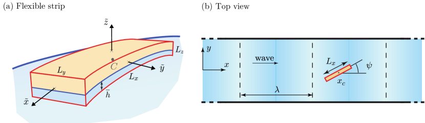
Figure 1: (a) Flexible strip with dimensions $L_{x},L_{y},L_{z}$, floating at the water surface with a constant immersion depth $\overline{h}$. (b) Top view of the strip drifting in a propagating wave. The yaw angle $\psi$ is the angle between the strip long axis and the direction of wave propagation.

The strip, sketched in Fig. 1(a), is a flexible rectangle of length, width and height ordered as $L_{x}\gg L_{y}\gg L_{z}$, and density $\rho_{s}<\rho$. Although the final result pertains to a thin strip, we need to consider a finite thickness in order to express the buoyancy force and torque in terms of volume integrals. We assume that the strip has zero bending rigidity in the thin direction, but is inextensible in the other directions, so that it follows exactly the surface of the waves. We can therefore consider that the strip is everywhere immersed at the equilibrium submersion depth $\overline{h}$, as shown in Fig. 1(a). We note that this equilibrium submersion depth is simply given by $\overline{h}=\rho_{s}L_{z}/\rho$ if only the buoyancy force is considered, but it can be slightly different because of capillary forces.

We parameterize the volume $V$ using curvilinear coordinates $(\tilde{x},\tilde{y},\tilde{z})$ along the long, middle and short axis, with $\tilde{x}\in[-L_{x}/2,L_{x}/2]$, $\tilde{y}\in[-L_{y}/2,L_{y}/2]$ and $\tilde{z}\in[-L_{z}/2,L_{z}/2]$. These coordinates are connected to the laboratory frame by

$$x\approx x_{c}(t)+\tilde{x}\cos\psi(t),\quad\quad y\approx y_{c}+\tilde{x}\sin\psi(t),\quad\quad z\approx\zeta(x,t).$$ (2)

The coordinates $x_{c}(t)$ and $y_{c}$ carry the horizontal position, and $\psi(t)$ denotes the yaw angle, i.e., the angle between the strip long axis and the direction of wave propagation, as shown in Fig. 1(b). We ignore the variation along $\tilde{y}$ and $\tilde{z}$ that are treated as short directions. The submerged volume $V_{sub}$ is parametrized using the same coordinates, except that $\tilde{z}\in[-L_{z}/2,-L_{z}/2+\overline{h}]$. The velocity of a point $\bm{r}$ on the strip is

$$\bm{v}\approx(\dot{x}_{c}-\dot{\psi}\tilde{x}\sin\psi)\bm{e}_{x}+\dot{\psi}\tilde{x}\cos\psi\bm{e}_{y}+\partial_{t}\zeta\bm{e}_{z}.$$ (3)

Equations of motion for $x_{c}(t)$ and $\psi(t)$ are given by Newton’s law ($x$-component) and the angular momentum theorem ($z$-component),

$$\frac{d}{dt}\underbrace{\left(\int_{V}\rho_{s}v_{x}\,dV\right)}_{=\,M\dot{x}_{c}}=F_{x},\quad\quad\frac{d}{dt}\underbrace{\left(\int_{V}\rho_{s}\,\bm{e}_{z}\cdot(\bm{r}-\bm{r}_{c})\times\bm{v}\,dV\right)}_{=\,I_{zz}\dot{\psi}}=K_{z},$$ (4)

with $M=\rho_{s}L_{x}L_{y}L_{z}$ the mass and $I_{zz}\approx ML_{x}^{2}/12$ the moment of inertia of the floater. We ignore capillary and viscous effects, and suppose that $F_{x}$ and $K_{z}$ is only due to the dynamic pressure of the incoming wave in the absence of floater. This hypothesis corresponds to the Froude-Krylov approximation, which neglects diffraction and radiation.

Denoting $d\bm{S}$ the surface element on the floater, towards the liquid, $S_{Sub}$ the submerged part of the floater surface and $V_{sub}$ the submerged volume, we then have

$$F_{x} = -\int_{S_{sub}}(p-p_{0})\bm{dS}\cdot\bm{e}_{x}=-\int_{V_{sub}}\partial_{x}p\,dV=\int_{V_{sub}}\rho\Big{(}\partial_{t}u_{x}+\underbrace{(\mathbf{u}\cdot\bm{\nabla})u_{x}}_{\sim\,\sin 2(kx-\omega t)}\Big{)}dV$$ (5a)

$$K_{z} = -\int_{S_{sub}}\left((\bm{r}-\bm{r}_{c})\times(p-p_{0})\bm{dS}\right)\cdot\bm{e}_{z}=-\int_{V_{sub}}\rho(y-y_{c})\Big{(}\partial_{t}u_{x}+\underbrace{(\mathbf{u}\cdot\bm{\nabla})u_{x}}_{\sim\,\sin 2(kx-\omega t)}\Big{)}dV.$$ (5b)

We have used the divergence theorem and Euler’s law to rewrite $F_{x}$ and $K_{z}$ using volume integrals. Injecting the flow profiles, we can compute these integrals. The underbraced terms involving $(\mathbf{u}\cdot\bm{\nabla})u_{x}\sim\sin 2(kx-\omega t)$ are negligible in what follows. Of second order in wave magnitude, they do not affect the first order motion of $x_{c}$ and $\psi$ and since they have a vanishing time-average, they do not influence the slow motion at second order.

II.2 First and second order mean motion

We scale space in units of $k^{-1}$, time in units $\omega^{-1}$, and mass in units $M$. We denote $\epsilon=ka$ the wave slope, $\delta_{x,y,z}=kL_{x,y,z}$ the non-dimensional floater size, and $\overline{\delta}_{h}=k\overline{h}$ the non-dimensional immersion depth. In non-dimensional units, the local fluid acceleration is $\partial_{t}u_{x}(x,z,t)=-\epsilon e^{z}\cos{(x-t)}$, and the surface elevation is $\zeta(x,t)=\epsilon\sin(x-t)$. For thin elongated strips, we can approximate the volume integrals over $V_{sub}$ as line integrals, yielding a non-dimensional force and moment

$$F_{x}\approx-\epsilon\overline{\delta}_{h}\delta_{y}\int_{-\delta_{x}/2}^{\delta_{x}/2}e^{z}\,\cos{(x-t)}\,d\tilde{x},\quad\quad K_{z}\approx\epsilon\overline{\delta}_{h}\delta_{y}\int_{-\delta_{x}/2}^{\delta_{x}/2}(y-y_{c})\,e^{z}\,\cos{(x-t)}\,d\tilde{x}.$$ (6)

We replace $x,y,z$ with (2) and notice that this force and moment can be rewritten in conservative form

$${F}_{x}\approx-\frac{\partial V}{\partial x_{c}},\quad\quad{K}_{z}\approx-\frac{\partial V}{\partial\psi}$$ (7)

by introducing a potential

$$V = \overline{\delta}_{h}\delta_{y}\int_{-\delta_{x}/2}^{\delta_{x}/2}e^{\epsilon\sin(x_{c}+c_{\psi}\tilde{x}-t)}\,d\tilde{x}$$ (8)

$$\approx \overline{\delta}_{h}\delta_{x}\delta_{y}\left\{1+\epsilon\operatorname{sinc}\left(c_{\psi}\frac{\delta_{x}}{2}\right)\sin(x_{c}-t)\right.\left.+\frac{\epsilon^{2}}{4}\left[1-\operatorname{sinc}\left(c_{\psi}\delta_{x}\right)\cos 2(x_{c}-t)\right]+O(\epsilon^{3})\right\}.$$

We denote in short $c_{\psi}=\cos\psi$. To get the second expression, we have expanded the exponential in the integrandum in powers of $\epsilon$, up to second order. The $O(\epsilon^{2})$ term in this potential is shown here, but it has no impact on the second order slow motion: the uniform and stationary part does not create motion and the term $\sim\cos 2(x_{c}-t)$ only creates second order harmonics. As a result, the first order harmonic motion and the second order, slow drift of $x_{c}$ and $\psi$ are determined by

$$\ddot{x}_{c}\approx-\frac{\partial}{\partial x_{c}}\left[\epsilon\operatorname{sinc}\left(\frac{\delta_{x}}{2}c_{\psi}\right)\sin(x_{c}-t)\right],\quad\quad\ddot{\psi}\approx-\frac{\partial}{\partial\psi}\left[\epsilon{\frac{12}{\delta_{x}^{2}}}\operatorname{sinc}\left(\frac{\delta_{x}}{2}c_{\psi}\right)\sin(x_{c}-t)\right].$$ (9)

We now expand the motion as $x_{c}\approx\overline{x}_{c}+x^{\prime}_{c}$, $\psi\approx\overline{\psi}+\psi^{\prime}$. The barred variables are $O(1)$ and we admit that they vary on the slow time scale $\tau=\epsilon t$, whereas the primed variables carry the $O(\epsilon)$ harmonic response of the floater to the wave. Injecting the expansion into the system and expanding in Taylor series, we find at order $O(\epsilon)$, differential equations for $x_{c}^{\prime}$ and $\psi^{\prime}$ that are readily integrated to

$$x^{\prime}_{c}=\epsilon\operatorname{sinc}\left(\overline{c}_{\psi}\frac{\delta_{x}}{2}\right)\cos(\overline{x}_{c}-t),\quad\quad\psi^{\prime}=\epsilon{\frac{12}{\delta_{x}^{2}}}\frac{\partial}{\partial\overline{\psi}}\left[\operatorname{sinc}\left(\overline{c}_{\psi}\frac{\delta_{x}}{2}\right)\right]\sin(\overline{x}_{c}-t).$$ (10)

Here $\overline{c}_{\psi}=\cos\overline{\psi}$. Averaging the $O(\epsilon^{2})$ problem over time, we find the equations for the slow variation of the mean variables:

$$\ddot{\overline{x}}_{c} = 0\hskip 42.67912pt\text{and}$$ (11)

$$\ddot{\overline{\psi}} = -\frac{\partial\overline{V}}{\partial\overline{\psi}},\quad\quad\text{with }\overline{V}=\frac{3\epsilon^{2}}{\delta_{x}^{2}}\left[\underbrace{\operatorname{sinc}^{2}\left(\overline{c}_{\psi}\frac{\delta_{x}}{2}\right)-1}_{\text{due to }x^{\prime}_{c}}\quad+\quad\underbrace{{\frac{12}{\delta_{x}^{2}}}\left(\frac{\partial}{\partial\overline{\psi}}\left[\operatorname{sinc}\left(\overline{c}_{\psi}\frac{\delta_{x}}{2}\right)\right]\right)^{2}}_{\text{due to }\psi^{\prime}}\right].$$ (12)

The equation on $\overline{x}_{c}$ implies a constant drift velocity that is calculated in section C.

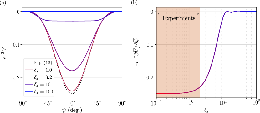
Figure 2: (a) Effective potential $\epsilon^{-2}\overline{V}$ (12) governing the mean yaw angle for various strip lengths $\delta_{x}$. The black dotted line represents the small $\delta_{x}$ limit (13). (b) Non-dimensional moment $-\epsilon^{-2}\partial\overline{V}/\partial\overline{\psi}$ for a mean yaw angle $\overline{\psi}=45^{\circ}$.

The slow rotation of $\overline{\psi}$ is therefore controlled by an effective potential $\overline{V}(\overline{\psi})$, which contains a contribution due to the fast back-and-forth displacement $x^{\prime}_{c}$ and a contribution due to the fast yaw oscillations $\psi^{\prime}$. The function $\epsilon^{-2}\overline{V}(\overline{\psi})$ is plotted in Fig. 2(a) for various strip lengths $\delta_{x}$. The minimum and maximum of $\overline{V}$ are always located at $\overline{\psi}=0^{o}$ and $\pm 90^{o}$, demonstrating that the longitudinal orientation $\overline{\psi}=0^{o}$ is always stable and the transverse orientation is always unstable. The minimum at $\overline{\psi}=0^{o}$ is well pronounced for small $\delta_{x}$, suggesting a robust stability of the longitudinal orientation for small strips. However, as $\delta_{x}$ is increased, the effective potential becomes gradually flatter, suggesting a weaker preference for the longitudinal orientation. This decreasing influence of waves on strips of large $\delta_{x}$ is better seen by computing the non-dimensional moment $-\epsilon^{-2}\partial\overline{V}/\partial\overline{\psi}$ for a fixed value of $\overline{\psi}$, here taken equal to 45^o (see Fig.  2b). It is systematically negative for short strips, indicating a slow rotation towards the longitudinal orientation $\overline{\psi}=0^{o}$, for which we can offer a simple physical interpretation. During the passage of each wave crest, the strip experiences a negative torque, causing it to rotate longitudinally, in the direction of wave propagation. Conversely, at each wave trough, a positive torque rotates the strip transversely. Due to the asymmetry in dynamic pressure, which is slightly larger at the crests than at the troughs, a small net negative torque is generated, favoring the longitudinal orientation. For $\delta_{x}>O(10)$, i.e. for $L_{x}>2\lambda$, the moment becomes essentially zero with small oscillations, which can be seen as a cancelling of the contributions of the large number of wave crests and troughs along the strip.

At this point, no assumption has been made on the strip length $\delta_{x}$. The short-strip limit, relevant to the experiments presented in the next section, provides an interesting simplification of the problem. In this limit, the effective potential (12) becomes

$$\overline{V}=-\frac{\epsilon^{2}}{4}\overline{c}_{\psi}^{4}+O(\epsilon^{2}\delta_{x}^{2}),$$ (13)

also plotted in Fig. 2(a) as the dotted line and clearly favors the longitudinal orientation. It is interesting to compare this effective potential for a flexible floater to the one obtained by Herreman et al. [17] for a rigid floater,

$$\overline{V}_{rigid}=-\frac{\epsilon^{2}}{4}\overline{c}_{\psi}^{4}\left(1-\frac{\delta_{x}^{2}}{60\overline{\delta}_{h}}\right).$$ (14)

The extra term in Eq. (14) produces a change of sign of $\overline{V}_{rigid}$ when the non-dimensional parameter $F=\delta_{x}^{2}/\overline{\delta}_{h}$ (or $kL_{x}^{2}/\overline{h}$) crosses the critical value 60. In other words, a long rigid floater with $F>60$ admits $\overline{\psi}=90^{o}$ (transverse orientation) as a stable equilibrium. We showed in Ref. [17] that this transverse equilibrium originates from the variation of the submersion depth along the floater length, which increases the torque in the trough positions, when the tips are more submersed. Because of the constant submersion depth for flexible floaters, this additional mechanism is absent, resulting in their systematic longitudinal orientation.

II.3 Drift velocity

In the previous section we have found that $\overline{F}_{x}=0+O(\epsilon^{3})$, resulting in $\ddot{\overline{x}}_{c}=0$. This suggests a constant drift velocity, which we compute as follows. We notice in the expression of the force $F_{x}$ (5a) that the time derivative can be taken outside the integral using Reynolds transport theorem. Equation (5a) can therefore be written as

$$F_{x}=\frac{d}{dt}\left(\int_{V_{sub}}\rho u_{x}\,dV\right)+\int_{V_{sub}}\rho\underbrace{\left((\bm{u}-\bm{v})\cdot\bm{\nabla}\right)u_{x}}_{\sim\,\sin(2(k\overline{x}_{c}-\omega t))}\,dV.$$ (15)

Here $\bm{v}$ is the velocity of the strip as defined in Eq. (3). The second term of Eq. (15) is of order $\epsilon^{2}$ and it can be shown, plugging in the first order movement $(x^{\prime}_{c},\psi^{\prime})$ of equations (10), that it does not contribute to the mean motion at second order of the wave amplitude. The equation for the translation $m\ddot{x}_{c}=F_{x}$ is then integrated once, yielding

$$m\dot{x}_{c}=\int_{V_{sub}}\rho u_{x}dV+cst.$$ (16)

The integration constant is defined by the initial conditions, and can take arbitrary values in a perfect fluid. However, if we want the model to recover the classical formula for the Stokes drift of material points (limit $V_{sub}\rightarrow 0$), we need to set this integration constant to zero. We nondimensionalize and calculate the integrals with the same techniques as before. This yields the equation

$$\dot{x}_{c}=\epsilon\operatorname{sinc}\left(c_{\psi}\frac{\delta_{x}}{2}\right)\sin(x_{c}-t)+\epsilon^{2}/2.$$ (17)

We inject $x_{c}=\overline{x}_{c}+x_{c}^{\prime}$ and $\psi=\overline{\psi}+\psi^{\prime}$ and Taylor expand the right hand side up to order $O(\epsilon^{2})$. At order $O(\epsilon)$, we retrieve the same first order movement $x^{\prime}_{c}$ as found in Eq. (10). At second order we inject the fast oscillating movement in translation ($x^{\prime}_{c}$) and rotation ($\psi^{\prime}$) in Eq. (17) and we find the mean velocity

$$\dot{\overline{x}}_{c} = \epsilon^{2}+\frac{\epsilon^{2}}{2}\left[\underbrace{\operatorname{sinc}^{2}\left(\overline{c}_{\psi}\frac{\delta_{x}}{2}\right)-1}_{\text{due to }x^{\prime}_{c}}\quad+\quad\underbrace{{\frac{12}{\delta_{x}^{2}}}\left(\frac{\partial}{\partial\overline{\psi}}\left[\operatorname{sinc}\left(\overline{c}_{\psi}\frac{\delta_{x}}{2}\right)\right]\right)^{2}}_{\text{due to }\psi^{\prime}}\right].$$ (18)

We note that the term in bracket is, with a factor $6/\delta_{x}^{2}$, identical to effective potential governing the angular drift (12). In the limit $\delta_{x}\rightarrow 0$, we recover the classical Stokes drift velocity for a material point, $\dot{\overline{x}}_{c}=\epsilon^{2}$ (or $\epsilon^{2}\omega/k$ in dimensional units). The term in brackets is the correction to Stokes drift due to finite size and orientation, and it is always negative according to this inviscid Froude-Krylov model. For infinitely long strips, it yields $\dot{\overline{x}}_{c}=\epsilon^{2}/2$, exactly half of the material-point Stokes drift. This result can be understood as follows: for very long strips the fast oscillating first order motion (10) vanishes ($x^{\prime}_{c}\rightarrow 0$ and $\psi^{\prime}\rightarrow 0$). The strips do not move in the horizontal direction on short time scales, but still deform vertically to adapt to the interface. Through this vertical motion, the vertical velocity gradients of the flow are seen by the strip and this results in a $\epsilon^{2}/2$ term that also appears in the derivation of the Stokes drift velocity of material points. Finally in the small strip limit that applies to our experiments, the drift velocity (18) simplifies to

$$\dot{\overline{x}}_{c}=\epsilon^{2}\left(1-\frac{1}{24}\delta_{x}^{2}{\overline{c}_{\psi}^{4}}\right)+O(\epsilon^{2}\delta_{x}^{4}).$$ (19)

This expression clearly shows a decrease of the drift velocity compared to the material-point Stokes drift prediction, which is more pronounced for a strip aligned along the direction of wave propagation.

II.4 Discussion

To summarize, we derived a set of coupled equations, (12) and (18), that describes the slow evolution of the strip velocity and yaw angle $(\dot{\overline{x}}_{c},\overline{\psi})$. We note that this coupling is unidirectional: the drift velocity $\dot{\overline{x}}_{c}$ depends on the mean yaw angle ${\overline{\psi}}$, but the evolution of $\overline{\psi}$ is independent of $\dot{\overline{x}}_{c}$. To solve for this set of equations, we must therefore first integrate in time the mean yaw angle from Eq. (12), and then compute the resulting drift velocity $\dot{\overline{x}}_{c}$ from Eq. (18). These coupled equations predict slow periodic oscillations of both $\overline{\psi}$ and $\dot{\overline{x}}_{c}$, at a frequency of order $\epsilon\omega$ that depends on the initial condition: the mean angle $\overline{\psi}(t)$ slowly oscillates around the stable fixed point $0^{o}$ (longitudinal orientation), while the drift velocity $\dot{\overline{x}}_{c}$ slowly oscillates around a mean value smaller than the material-point Stokes drift $\epsilon^{2}$, with a lower bound at $\epsilon^{2}(1+\operatorname{sinc}^{2}(\delta_{x}/2))/2$.

These periodic oscillations directly follow from the assumption of inviscid dynamics, and are not expected in a realistic experiment with dissipation. Including dissipation in the model would probably yield damped oscillations converging toward $\overline{\psi}=0^{o}$, together with a final drift velocity in principle smaller than $\epsilon^{2}$. While the first prediction for the constant longitudinal orientation $\overline{\psi}=0^{o}$ seems natural, the second prediction for a reduced drift velocity is questionable: viscosity is known to increase the drift velocity of an extended flexible sheet [21, 22], to an amount that may exceed the reduction predicted here.

III Experiments

III.1 Experimental setup

We have performed a series of laboratory experiments to study the slow motion of flexible floaters drifting in surface waves. Experiments were conducted in a rectangular water channel sketched in Fig. 3(a). The tank is $4$ m long, $18$ cm wide, and is filled with water at height $H=22$ cm. Waves are generated by a piston-type wavemaker oscillating at a frequency $f=\omega/2\pi$ between 1 and 2 Hz, corresponding to wavelengths in the range $\lambda\simeq 0.4-1.2$ m, and are attenuated at the end of the tank by a sloping beach. In this range of frequencies, capillary effects can be neglected, and the waves obey the gravity-wave dispersion relation in finite depth, $\omega^{2}=gk\tanh{kH}$. For each frequency, the wave amplitude $a$ is chosen so that the slope remains approximately constant, $\epsilon=ak\simeq 0.14\pm 0.01$. This value is sufficiently large to create a significantly rapid drift and reorientation, and keeps the waves within the linear regime.

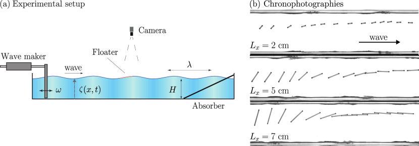
Figure 3: Experimental setup. (a) Side view. A $4$ m long, $18$ cm large wave tank is filled at height $H=22$ cm. A wave maker oscillates at a frequency $\omega$, generating waves of velocity $c$ and wavelength $\lambda$. (b) Chronophotographies of flexible strips of varying lengths $L_{x}$, taken at intervals of three wave periods, showing their systematic orientation along the direction of the wave propagation.

The floaters are rectangular strips of width $L_{y}=5$ mm and lengths $L_{x}$ ranging from $1$ to $13$ cm (corresponding to $\delta_{x}=kL_{x}\simeq 0.1-2$), cut from polypropylene sheets of thickness $L_{z}\approx 53\pm 1$ $\mu$m and surface density $\rho_{\sigma}=48\pm 1$ g/m². At rest, such thin strips lay flat at the water surface, due to the combined effects of capillary forces and rigidity. Capillary forces at the perimeter of the strip induce a tension $\gamma\approx 0.07$ N/m, and the rigidity is characterized by the bending modulus

$$D=\frac{EL_{z}^{3}}{12(1-\nu^{2})}\approx(1.5\pm 0.2)\,10^{-6}\text{ N~{}m,}$$

with $E$ the Young’s modulus and $\nu$ the Poisson coefficient ($E\approx 0.09\pm 0.01$ GPa and $\nu\approx 0.5$ for poylpropylene). Gravity waves are unaffected by the tension $\gamma$ in the strip and its rigidity $D$ if [23]

$$|\rho g\zeta|\gg|\gamma\partial^{2}_{xx}\zeta|,\,|D\partial^{4}_{xxxx}\zeta|.$$

This requires wavelengths much larger than both the flexural-gravitary wavelength and the gravito-capillary wavelength,

$$\lambda\gg\lambda_{gD}=2\pi\left(\frac{D}{\rho g}\right)^{1/4}\approx 2.2~{}\mbox{cm},\quad\text{and}\quad\lambda\gg\lambda_{gc}=2\pi\sqrt{\frac{\gamma}{\rho g}}\approx 1.7~{}\mbox{cm}.$$

With $\lambda$ in the range $0.4-1.2$ m in our experiments, these approximations are comfortably satisfied, indicating that the strips can be considered as infinitely bendable and that they perfectly adapt to the surface shape.

III.2 Tracking and drift velocity

Experiments to investigate the orientation dynamics and drift velocity of floating strips are conducted as follows. A strip is cautiously deposited on the water surface at rest, at an initial yaw angle $\psi$ in the range $60-80^{o}$, ensuring no air bubbles are trapped beneath it. The wave maker is switched on and the motion of the strip is recorded during approximately 1 minute using a camera located above the wave tank. We repeat the experiments several times for each strip length, and retain trajectories that remain approximately centered in the channel to discard possible interaction with the side walls. After each run, we wait approximately 10 minutes for the waves and currents to dissipate.

The chronophotographies in Fig. 3(b), obtained by superimposing images at intervals of three wave periods, illustrate the motion of the strip for three different lengths, $L_{x}=2,5$ and 7 cm. We observe a reorientation of the strips in the direction of the wave propagation, in good agreement with the theoretical prediction. All experiments, carried out with varying strip lengths $L_{x}$ and wave frequencies $f$, systematically demonstrated longitudinal orientation.

To further characterize the motion of the strip, we measure on each frame the position of its center of mass $x_{c}$ and its yaw angle $\psi$ using the TrackMate plug-in of ImageJ. This is done by tracking the position of two black dots located at each end of the strip. An example of time series of $x_{c}(t)$ and $\psi(t)$ is given in Fig. 4 for a strip of length $L_{x}=8$ cm. Both quantities clearly show rapid first-order oscillations at the wave frequency, superimposed to slow second-order trends. The yaw angle shows a slow decrease, followed by small erratic motions around the longitudinal direction $\psi=0\pm 10^{\circ}$.

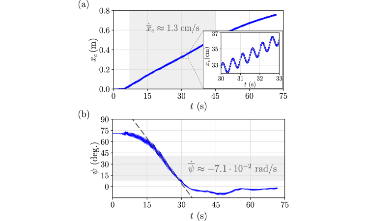
Figure 4: (a) Position and (b) yaw angle of a strip of length $L_{x}=8$ cm drifting in a wave of frequency $f=2$ Hz, wavelength $\lambda=0.39$ m, and wave slope $ak=0.14$. The mean angular velocity is shown as a dashed line.

In Fig. 4(a), we see that the strip rapidly acquires a nearly constant drift velocity $\dot{\overline{x}}_{c}$ once the waves are established, approximately 5 s after the start of the wavemaker, but it significantly decelerates after $t\simeq 45$ s. This slower drift is likely due to the gradual development of a streaming flow, originating from the diffusion of vorticity produced in the oscillating boundary layers into the bulk [24, 25]. The resulting correction to the mean flow, which occurs typically after 45 s in our experiments, limits the duration of each run. In the following, the drift velocity is computed in this first time interval, where it is approximately constant. In the example shown in Fig. 4(a), we obtain $\dot{\overline{x}}_{c}\approx 1.3\pm 0.2$ cm s^-1, a value close to the expected Stokes drift of a point particle, $c\epsilon^{2}\approx 1.5$ cm s^-1 (with $c=\omega/k$ the phase velocity). This small discrepancy can be explained by the influence of the return flow, unavoidably present in a tank of finite depth: Mass conservation requires a zero flow rate through any vertical cross section, implying that a negative flow takes place to balance the positive Stokes drift [16]. With the assumption of a homogeneous return flow, we expect a correction of the order of $c\epsilon^{2}/(2kH\tanh{kH})$, resulting in a $10$ to $20\%$ reduction in the net Eulerian surface velocity, close to what we observe experimentally.

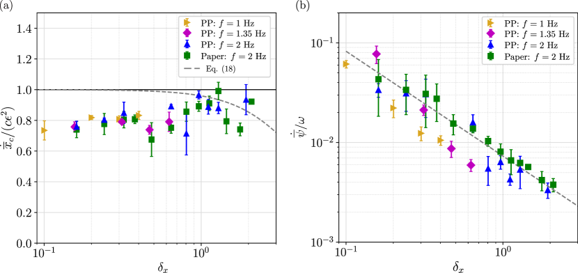
Figure 5: (a) Normalized drift velocity $\dot{\overline{x}}_{c}/(c\epsilon^{2})$ as a function of the non dimensional length $\delta_{x}=kL_{x}$ (PP: polypropylene). The full line at 1 is the expected material-point Stokes drift, and the dashed line is the predicted drift velocity for a floater in the longitudinal orientation [Eq. (18) evaluated for $\overline{\psi}=0^{o}$]. (b) Normalized angular velocity $\dot{\overline{\psi}}/\omega$ as a function of $\delta_{x}$. The dashed line shows the power law (20).

We repeated the experiment for strips of various lengths and for various wave frequencies, and show in Fig. 5(a) the normalized drift velocity $\dot{\overline{x}}_{c}/(c\epsilon^{2})$ as a function of the normalized length $\delta_{x}=kL_{x}$. Each point is calculated as the average over three to ten measurements, with error bars representing the standard deviations. Our measurements show a systematic deviation of $10-20\%$ below the material-point Stokes drift prediction $\dot{\overline{x}}_{c}/(c\epsilon^{2})=1$, consistent with the expected return flow contribution. In this figure we also show in dotted line the lower bound of the predicted drift velocity (18) for a perfectly longitudinal strip, $\dot{\overline{x}}_{c}/(c\epsilon^{2})=(1+\operatorname{sinc}^{2}(\delta_{x}/2))/2$. In the range of strip lengths considered here, $\delta_{x}=0.1-2$, this correction is less than 15%, and falls within the uncertainties due to the return flow and possibly to early streaming effects. We can conclude that the measured drift velocities, within the experimental precision, are indistinguishable from the simple material-point Stokes drift prediction.

III.3 Reorientation dynamics

We now turn to the orientation dynamics of the strips. Our systematic observations of longitudinal orientation for all strip lengths is consistent with the theoretical prediction of a stable fixed point of the effective potential at $\overline{\psi}=0^{o}$. However, the theory predicts periodic oscillations around this stable fixed point, while experiments show a relaxation toward $\overline{\psi}=0^{o}$. This relaxation must originate from dissipation, not considered in the theory, likely from the viscous boundary layer beneath the strips, or to a lesser extent from wave emission.

To characterize this relaxation dynamics, we measure the mean angular rate $\dot{\overline{\psi}}$ by a linear fit of $\psi(t)$ in a time interval such that it decreases approximately linearly, as illustrated in Fig. 4(b). In practice, we observe that between $40^{\circ}$ and $10^{\circ}$ the decrease is linear and independent of the initial condition. We note that this range occurs within the time interval during which the drift velocity is constant. The resulting (absolute) angular velocity $\dot{\overline{\psi}}$ normalized by the wave frequency $\omega$ is plotted in Fig. 5(b) as a function of the normalized length $\delta_{x}=kL_{x}$. Here again, the error bars represent the standard deviations from 3 to 10 experiments. We observe a good collapse of the data, compatible with a power-law $\delta_{x}^{-1}$. To account for the slow time scale $\epsilon\omega^{-1}$ of the reorientation dynamics, we write this power law in the form

$$\frac{\dot{\overline{\psi}}}{\omega}\simeq\alpha\epsilon\delta_{x}^{-1}.$$ (20)

Fitting our data with this law gives $\alpha\simeq(7\pm 1)\,10^{-3}$.

To check the robustness of our observations, we have repeated the experiments with rectangular strips of paper, with the same width $L_{y}$ and range of lengths $L_{x}$ as before. The surfacic density of dry paper is $\rho_{\sigma}=80$ g/m² but, contrary to polypropylene, paper absorbs water, so the relevant surface density is that of wet paper, $\rho_{\sigma}\approx 180\pm 10$ g/m² (we estimate $\rho_{\sigma}$ by first soaking the paper strip in water and then weighing it, ensuring that no excess water droplets are present). We note that paper is heavier than water, so its flotation is ensured by capillary forces. The rigidity of wet paper is comparable to that of polypropylene, $D\approx(1.1\pm 0.5)\times 10^{-6}$ N m, resulting in a similar flexural-gravitary crossover wavelength, $\lambda_{gD}\approx 2$ cm. Experiments with these paper strips also show a systematic longitudinal orientation, with mean angular rates $\dot{\overline{\psi}}/\omega$, plotted in Fig. 5(b), in good agreement with that of polypropylene strips. This is consistent with our model, which predicts that the value of the immersion depth does not affect the angular dynamics of the strips, the only requirement being that they remain at the surface and deform with the waves.

Finally, we note that our results are also consistent with the qualitative observations of Wong et al. [13] performed with polyethylene sheets of elliptical shape. The authors also report a systematic trend for longitudinal orientation. From the images they provide in their paper for the parameters $f=0.98$ Hz, $ak=0.165$ and $\delta_{x}\approx 4.0$, we estimate a re-orientation rate $\dot{\overline{\psi}}/\omega\approx 5.10^{-4}$. This value is consistent with our data, although twice smaller than our empirical fit (20). This can be explained by the fact that floaters start from $\overline{\psi}\approx 90^{\circ}$ in the study of Wong et al., and for these angles we expect a much smaller yaw moment.

IV Conclusion

In this paper, we introduced a Froude-Krylov model to describe the slow motion of a thin flexible strip drifting in surface gravity waves. This model predicts a mean yaw moment that favors a longitudinal orientation of the strip, in the direction of wave propagation, and a small reduction of the drift velocity compared to the material-point Stokes drift. We performed laboratory experiments using strips of polypropylene of various lengths, that confirm the systematic longitudinal orientation, but cannot confirm the small reduction in drift velocity because of limited resolution. Although our experiments are performed for centimeter-scale strips, close to the capillary-gravity wavelength, capillary forces are not expected to play a significant role in the second-order forces and moments acting on the strip, suggesting that our results should hold for large-scale flexible structures.

The systematic longitudinal orientation of flexible floaters strongly differs from the behavior found for rigid floaters. While short and heavy rigid floaters also show a preferential longitudinal orientation, long and light rigid floaters orient transversely, parallel to the wave crests [17]. This transverse equilibrium arises from the variation of the submersion depth along the long axis of the floaters, which significantly increases the yaw moment in the trough positions. Since there is no variation in the submersion depth for perfectly flexible floaters, this additional mechanism is absent, resulting in their systematic longitudinal orientation. This difference between rigid and flexible floaters suggests a change in behavior governed by the bending rigidity of the floater. For floaters of intermediate rigidity, a situation relevant to large floating structures or ice floes [10], the hydroelastic response of the structure should result in a variable immersion depth along the floater, and we expect a behavior between the flexible and rigid limits, i.e., a longitudinal-transverse transition governed by the floater length, density and rigidity.

Finally, our experiments suggest that the mean angular velocity of flexible floaters toward the stable longitudinal orientation decreases as $L_{x}^{-1}$, with $L_{x}$ the floater length. This effect is likely due to dissipation, and is not accounted for in our inviscid model, which predicts slow periodic oscillations around the longitudinal orientation. Introducing dissipation in our model would require a detailed resolution of the second-order flow in the oscillating boundary layer beneath the floater. This approach was only considered for infinite floating sheets, yielding an increased drift velocity induced by the streaming in the oscillating boundary layer [21, 22]. Extending this approach to flexible floaters of finite size that are not aligned with the direction of wave propagation is necessary to provide a full description of their slow second-order angular dynamics, but would represent a considerable task.