Through the Looking Glass:
Mirror Schrödinger Bridges
Abstract
Resampling from a target measure whose density is unknown is a fundamental problem in mathematical statistics and machine learning. A setting that dominates the machine learning literature consists of learning a map from an easy-to-sample prior, such as the Gaussian distribution, to a target measure. Under this model, samples from the prior are pushed forward to generate a new sample on the target measure, which is often difficult to sample from directly. In this paper, we propose a new model for conditional resampling called mirror Schrödinger bridges. Our key observation is that solving the Schrödinger bridge problem between a distribution and itself provides a natural way to produce new samples from conditional distributions, giving in-distribution variations of an input data point. We show how to efficiently solve this largely overlooked version of the Schrödinger bridge problem. We prove that our proposed method leads to significant algorithmic simplifications over existing alternatives, in addition to providing control over in-distribution variation. Empirically, we demonstrate how these benefits can be leveraged to produce proximal samples in a number of application domains.
1Massachusetts Institute of Technology 2Columbia University
1 Introduction
Mapping one probability distribution to another is a central technique in mathematical statistics and machine learning. Myriad computational tools have been proposed for this critical yet often challenging task. Models and techniques for optimal transport provide one class of examples, where methods like the Hungarian algorithm (Kuhn, 1955) map one distribution to another with optimal cost. Adding entropic regularization to the static optimal transport problem yields efficient algorithms like Sinkhorn’s method (Deming & Stephan, 1940; Sinkhorn, 1964), which have been widely adopted in machine learning since their introduction by Cuturi (2013). Static entropy-regularized optimal transportation is equivalent to a dynamical formulation known as the Schrödinger bridge problem (Schrödinger, 1932; Léonard, 2014), which has proven useful to efficiently compute an approximation of the optimal map paired with an interpolant between the input measures.
Inspired by these mathematical constructions and efficient optimization algorithms, several methods in machine learning rely on learning a map from one distribution to another. Beyond optimal transport, diffusion models, for instance, learn to reverse a diffusion process that maps data to a noisy prior. Special attention has been given to learning methods that accomplish this in a stochastic manner, i.e., modeling the forward noising process using a stochastic differential equation (SDE).
The most common learning applications of distribution mapping attempt to find a map from a simple prior distribution and a complex data distribution, either using a score-matching strategy (Song & Ermon, 2019; Ho et al., 2020; Song et al., 2021) or leveraging a formulation of the Schrödinger bridge problem (De Bortoli et al., 2021; Shi et al., 2022; 2023; Zhou et al., 2024); other learning applications map one complex data distribution to another (Cuturi, 2013; Courty et al., 2017).
In this paper, we focus instead on the understudied problem of mapping a probability distribution to itself, that is, finding a joint distribution whose marginals are both the same data distribution . This task might seem inane at first glance, since two simple couplings satisfy our constraints: one is the independent coupling , and the other is the “diagonal” map given by . The space of couplings between a measure and itself, however, is far richer than these two extremes and includes models whose conditional distributions are neither identical nor measures.
We focus on the class of self-maps obtained by entropy-regularized transport from a measure to itself. Formally, we define a mirror Schrödinger bridge to be the minimizer of the KL divergence over path measures with both initial and final marginal distributions equal to , where is an Ornstein-Uhlenbeck process with noise . Mirror Schrödinger bridges are the stochastic counterpart to minimizing , where is the probability density of the joint distribution associated with the path measure , over the joint distributions on satisfying the linear constraints and . While the former minimizes the Kullback-Leibler divergence on path space, the latter is a minimization over density couplings.
Despite its simplicity, this setting of the Schrödinger bridge problem suggests a rich application space. Couplings with the same marginal constraints have already proven useful to enhance model accuracy in vision and natural language processing by reinterpreting attention matrices as transport plans (Sander et al., 2022). Few works, however, consider this task from the perspective of optimizing over path measures or provide control over the entropy of the matching at test time. Albergo et al. (2023) propose a stochastic interpolant between a distribution and itself, but their interpolants are not minimal in the relative entropy sense and do not solve the Schrödinger bridge problem, even with optimization. Minimal interpolants in the relative entropy sense are those with minimal kinectic energy, and in applications, minimizing the kinectic energy of a path has been correlated to faster sampling (Shaul et al., 2023).
Contributions. We investigate the mirror Schrödinger bridge problem and demonstrate how it can be leveraged to obtain in-distribution variants of a given input sample. In particular, given a sample , we build a stochastic process with minimal relative entropy under which the sample arrives at some with proximal but not identical to .
Our contributions in this direction are twofold: first, on the theoretical side, we use the time symmetry of the mirror Schrödinger bridge to prove that it can be obtained as the limit of iterates produced via an alternating minimization procedure; and second, in applications, the implementation of our method allows for sampling from the conditional distribution in such a way that we can control how proximal a generated sample is relative to the input sample .
2 Related Works
Entropy regularized optimal transport. A few recent works employ the idea of a coupling with the same marginal constraints. Feydy et al. (2019); Mensch et al. (2019) use static entropy-regularized optimal transportation from a distribution to itself to build a cost function correlated to uncertainty. Sander et al. (2022) reinterpret attention matrices in transformers as transport plans from a distribution to itself, while Agarwal et al. (2024) analyze this reinterpretation in the context of gradient flows. Also relevant is the work of Kurras (2015), who shows that, over discrete state spaces, Sinkhorn’s algorithm can be simplified in the case of identical marginal constraints. These works do not consider the coupling with the same marginal constraints from the perspective of path measures on continuous-state spaces. In our paper, we focus on the path measure formulation instead of viewing it as a self-transport map and present a practical algorithm to solve it.
Expectation maximization. Our methodology can be broadly categorized under the umbrella of expectation maximization algorithms, drawing from the theory of information geometry. A number of recent papers introduce related formulations to machine learning; most relevant to us are the works of Brekelmans & Neklyudov (2023); Vargas & Nüsken (2023). These works, however, focus on the case of finding a path measure with two distinct marginal constraints, overlooking the potential application to resampling and algorithmic simplifications obtained for the case in which the marginal constraints are the same. In our work, we derive an algorithm that is distinct, yet similar in flavor, to address this overlooked version of the problem, i.e. the mirror Schrödinger bridge.
Schrödinger bridges and stochastic interpolants. Schrödinger bridges have been used to obtain generative models by flowing samples from a prior distribution to an empirical data distribution from which new data is to be sampled. Several methods have been proposed to this end: De Bortoli et al. (2021); Vargas et al. (2021) iteratively estimate the drift of the SDE associated with the diffusion processes of half-bridge formulations. While the first uses neural networks and score matching, the latter employs Gaussian processes. From these, a number of extensions or alternative methods have been presented; most relevant are (Shi et al., 2023; Peluchetti, 2023), which extend (De Bortoli et al., 2021) but differ with respect to the projection sets used to define their half-bridge formulations.
To the best of our knowledge, the work of Albergo et al. (2023) is the only one in the literature on generative modeling that maps from a distribution to itself. In their paper, flow matching learns a drift function associated with a stochastic path from the data distribution to itself. Their stochastic interpolants, however, are not optimal with respect to any functional. In particular, they lack optimality in the relative entropy sense, a property correlated to sampling effectiveness and generation quality (Shaul et al., 2023) and hence of practical importance. By contrast, our method discovers the coupling with minimal relative entropy, akin to methods such as (De Bortoli et al., 2021; Shi et al., 2023); our method, however, presents certain algorithmic advantages over these, which can only be derived for the mirror case.
3 Mathematical Preliminaries
Definition. Let be an integer, and let be a reference measure in the space of path measures. Following (Jamison, 1975; Léonard, 2014), we define the Schrödinger bridge problem to be the problem of finding a path measure interpolating between prescribed initial and final marginals and that is the closest to the reference measure with respect to the Kullback-Leibler divergence . To be precise, we define to be the solution of the following optimization problem:
| (1) |
where denotes the set of path measures with marginals and . In other words, we say that is the direct projection of onto the space .
The reference path measure is typically chosen to be associated with a diffusion process, which is defined to be any stochastic process governed by a forward SDE of the form
where denotes the forward drift function, is the noise coefficient, and denotes the Wiener process. Such a process corresponds to a unique path measure once an initial or final condition is specified. An important aspect of diffusion processes is that their time-reversals are diffusion processes of the same noise coefficient . Specifically, if is a diffusion process with time-reversal denoted by , then is governed by a backward SDE of the form
where denotes the backward drift function (see (Winkler et al., 2023, section 2.3)).
In the case where arises from a diffusion process, any path measure with finite KL divergence with respect to , including the Schrödinger bridge , necessarily also arises from a diffusion process with noise (Vargas et al., 2021). Consequently, by adjusting the initial condition of the reference SDE, we can assume that the reference process has a prescribed initial marginal , without changing the solution to (1).
Iterative Proportional Fitting Procedure. In the literature, the typical strategy for solving the problem (1) is to apply a general technique known as the Iterative Proportional Fitting Procedure (IPFP) (Fortet, 1940; Kullback, 1968). This procedure obtains the Schrödinger bridge by iteratively solving the following pair of half-bridge problems:
| (2) |
where , respectively, , denotes the space of path measures with final (resp., initial) marginal fixed to be (resp., ). Ruschendorf (1995) proves that the sequence of iterates converges in total variation to as . IPFP can be thought of as an extension of Sinkhorn’s algorithm to continuous state spaces, where the rescaling updates characteristic of Sinkhorn are replaced by iterated direct projections onto sets of distributions with fixed initial or final marginal (Essid & Pavon, 2019).
Applications. Suppose is given by a data distribution and take to be an easy-to-sample distribution , e.g., . The backward diffusion process associated with gives a model for sampling from . In practice, the IPFP iterates in (2) can be solved using an algorithm known as the diffusion Schrödinger bridge (DSB), developed by De Bortoli et al. (2021). DSB relies on the following observation, which is a consequence of Girsanov’s theorem: is the path measure whose backward drift is equal to the time-reversal of the forward drift of , and is the path measure whose forward drift is equal to the time-reversal of the backward drift of . Leveraging this fact, DSB solves for by training neural networks to learn the forward and backward drift functions associated with the IPFP iterates.
4 Mirror Schrödinger Bridges
Given a reference path measure and a prescribed marginal distribution , we consider the Schrödinger bridge problem between and itself with respect to . In the case where is time-symmetric, the Schrödinger bridge will inherit the time-symmetry, in which case we call it the mirror Schrödinger bridge from to itself with respect to . Mathematically, we write
| (3) |
so that is the path measure with identical prescribed marginals equal to that is closest to the reference measure with respect to the KL divergence .
A naïve approach to solving the mirror Schrödinger bridge problem (3) is to apply IPFP with both marginals set equal to . In practice, this requires iterative training of two neural networks and , the first modeling the drift of the forward diffusion process associated to and the latter modeling the drift of the corresponding backward process. But this straightforward application of IPFP leads to unnecessary computational expense, as it fails to use the time-symmetry of the problem (3). In particular, at optimality the forward and backward drifts of must be equal, because the mirror Schrödinger bridge is time-symmetric.
In section 4.1, we develop a method for solving (3) by leveraging time-symmetry in conjunction with a general technique from information geometry known as the Alternating Minimization Procedure (AMP), which was first formalized by Csiszár & Tusnády (1984). Then, in section 4.3, we derive an efficient algorithm that involves training a single neural network modeling the drift of the diffusion process associated to and requires half of the computational expense in terms of training iterations for the mirror problem, when compared to other IPFP-based algorithms.
4.1 Alternating Minimization Procedure
Take the reference path measure to be time-symmetric. As an example, we can take to be associated to an Ornstein–Uhlenbeck process given by an SDE of the form , for , or more generally any reversible diffusion process. We propose the following iterative scheme:
| (direct projection) | (4) | |||
| (reverse projection) | (5) |
where is the set of time-symmetric path measures with no marginal constraints. This scheme is an instance of AMP and differs from IPFP in that it alternates between direct and reverse projections. To see this, note that (4) is a direct projection and coincides with the odd-numbered steps in the IPFP iterations (2), whereas (5) is a reverse projection, as the KL divergence is being computed against the optimization parameter instead of the previously produced path measure . That is to say, each iteration of the AMP scheme in (4)-(5) is designed to obtain the time-symmetric measure that minimizes the objective while remaining close in KL divergence to the measure obtained in the previous half iteration, which satisfies the initial marginal constraint .
It is natural to ask why we consider reverse projections, as opposed to direct projections, onto the space of symmetric path measures. In fact, replacing (5) with a direct projection would result in a viable symmetrized variant of IPFP, and by (Ruschendorf, 1995), the resulting iterates would converge in total variation to the mirror Schrödinger bridge. The difficulty is in computing the direct projection of a path measure onto . As we will demonstrate in section 4.3, it is considerably easier to compute the reverse projection onto , as this particular projection can be done completely analytically.
4.2 Convergence
For the scheme in steps (4)-(5) to be practical, we must prove that the iterates converge to the mirror Schrödinger bridge . The pointwise convergence of schemes like steps (4)-(5) was established by Csiszár & Tusnády (1984) in the special case where the state space is finite. In our setting, however, we work with infinite state spaces of the form for some dimension . In the following theorem, we prove that the sequence obtained in the AMP scheme converges in total variation to the mirror Schrödinger bridge, without relying on the finiteness assumption for the state space. To our knowledge, this result has not been established previously in the literature.
Theorem 1.
Our proof strategy for Theorem 1 is inspired by the convergence proofs for IPFP given in (Ruschendorf, 1995, Proposition 2.1) and (De Bortoli et al., 2021, Theorem 36). The basic idea is to prove that the sequence is Cauchy with respect to the metric induced by total variation; we then conclude using completeness of the space of path measures together with optimality of the Schrödinger bridge. The crucial distinction between our setting and theirs is that one of our projections is reversed, which presents an additional complication for establishing convergence to the mirror Schrödinger bridge. To overcome this challenge, we make use of an observation made by Vargas & Nüsken (2023, section 4.1 and proof of Proposition 4.1): in traditional IPFP, we can reverse one or both of the direct projections (2) while preserving the sequence of iterates obtained. In particular, they prove:
Lemma 2.
Let be probability distributions on , and let be any path measure. Then we have the following identities relating direct to reverse projections:
Using Lemma 2, we obtain the following result, which states that the Schrödinger bridge can be equivalently defined in terms of reverse . We defer the proof to Appendix A.
Proposition 3.
Let be probability distributions on and let be any path measure. Then the Schrödinger bridge with respect to is the unique solution to the following pair of optimization problems:
Proof of Theorem 1.
Equipped with Lemma 2, we can reverse the projections in the steps given by (4). Then we obtain the following sequence of pairs of reverse projections:
| (reverse projection) | |||
| (reverse projection) |
We apply the Pythagorean theorem for reverse projections, which shows that
| (6) |
Since KL divergences are always nonnegative, the sequence of partial sums in (6) is nondecreasing and bounded, so the sum must converge. Thus, for any , we can choose sufficiently large to ensure that for all . By Pinsker’s Inequality, we have that the same property holds with replaced by , i.e., the metric induced by total variation. Thus, the sequence is Cauchy with respect to . Since the space of path measures is complete with respect to this metric, there exists a limit . But just as we argued in the proof of Proposition 3, we can show that , so by uniqueness of the Schrödinger bridge with respect to reverse , as shown in Proposition 3, it follows that . ∎
4.3 Practical Algorithm
In this section, we describe an algorithm to solve the mirror Schrödinger bridge problem numerically, based on the AMP scheme that we introduced in section 4.1. We choose our reference path measure to be associated to an Ornstein-Uhlenbeck process given by an SDE of the form , for .
Recall that our proposed AMP scheme alternates between direct projections on the set of path measures with a prescribed initial marginal distribution and reverse projections on the set of time-symmetric path measures. We now explain how each of these projections is computed in practice. Our algorithm then follows by iteratively applying this pair of projections and is summarized in Algorithm 1.
Direct projection. We can compute the projection onto the set of path measures with a prescribed initial marginal distribution following the trajectory-caching method developed and applied in (Vargas et al., 2021; De Bortoli et al., 2021). Let be a probability distribution on , and let and be path measures corresponding to diffusion processes. Write and for the forward and backward drift functions corresponding to , and write for the drift of . As a consequence of Girsanov’s theorem, we can write explicitly in terms of and , or equivalently in terms of and ; for references, see (Chen et al., 2016, section 3) as well as (Winkler et al., 2023, sections 2.2, 2.3). Indeed, for some constants , we have
| (7) | ||||
| (8) |
In light of the identities (7) and (8), and because drift functions are much more amenable to modeling and estimation than path measures, it is convenient to recast the steps of our AMP scheme as iterative computations of drift functions associated to projections.
It follows immediately from (7) that the direct projection of onto the space is given by the unique path measure with initial marginal and forward drift equal to the drift of . In our AMP scheme, we employ this by taking to have drift equal to that of for each . But as we will see in our analysis of the reverse projection, it does not suffice for us to know only the forward drift associated to our path measure iterates. We need to know the backward drift too, but in practice, we do not have access to it. We use trajectory caching to estimate the backward drift . Trajectory caching is principled on the fact that can be expressed in terms of the expected rate of change in over time. Concretely, we have the following formula, which can be taken as a formal definition of the backward drift of a diffusion process:
| (9) |
To apply (9) in practice, take a positive integer and let be a sequence of discrete time steps with sequence of partial sums . Then we construct a discrete representation of the stochastic process by using the Euler-Maruyama method to generate a collection of sample trajectories starting at the initial distribution in accordance with the SDE , where we know the forward drift because we matched it to the drift of . Explicitly, we have for all and that
| (10) |
The limiting quantity in (9) is then leveraged as the target of the loss function used to train a neural network , which approximates the backward drift for a specified range of values . Specifically, we define the following loss function in terms of the optimization parameter :
| (11) |
Observe that the first two terms in the loss constitute the difference between the drift and the infinitesimal rate of change of the process , i.e., the discretization of the difference between the left- and right-hand sides of (9). The network parameters are then learned via gradient descent with respect to the loss function . The resulting function , where minimizes the loss , approximates the desired backward drift, as is suggested by De Bortoli et al. (2021, Proposition 3).
Reverse projection. We now describe how to compute the reverse projection onto the set of time-symmetric path measures. We are interested in computing the associated time-symmetric drift, rather than the path measure itself. To this end, let be a probability distribution on , and let and be path measures corresponding to diffusion processes. Suppose we seek to minimize over all . Using (7) and (8), we can write explicitly in terms of the forward and backward drift functions of the SDE corresponding to the path measures and . A key benefit of considering the reverse projection is that the expectation values in (7) and (8) are taken with respect to the fixed path measure , and not with respect to the varying path measure . This allows us to apply calculus of variations to compute a closed-form expression for the drift of the minimizer of over . First, observe that we can combine (7) and (8) to rewrite in a time-symmetric formulation as follows:
where is a constant. Note that the sum of squares inside the expectation on the right-hand side above is always nonnegative. Consequently, to minimize , it suffices to choose so that it minimizes this sum of squares pointwise everywhere. Taking the first variation of this sum of squares with respect to , setting the resulting expression equal to zero, and solving for the optimal , we find that
| (12) |
That is, the choice of minimizing has drift function given by the average of the forward and backward drifts of .
In our AMP scheme, we employ (12) by taking the forward and backward drifts corresponding to and averaging them to obtain the drift of the symmetric path measure . Practically speaking, if the drift of is a parametrized by a neural network for each , we take the drift of to be the average of the outputs of the neural networks and . In Algorithm 1, we denote the limiting drift as .
4.4 Sampling with In-distribution Variation
In this section, we provide a short intuitive explanation of how our method allows for resampling with prescribed proximity to an input sample. Given such a sample , we solve the SDE corresponding to the Schrödinger bridge to push forward in time, arriving at a final sample . We want to be a variation of , where the proximity of to correlates with the size of the noise coefficient . Justifying this mathematically requires understanding how the conditional distribution , specifically its mean and variance, depend on . While these quantities do not in general have closed form expressions, it is possible to compute them exactly in the case where is a -dimensional Gaussian.
In this case, let denote the diffusion process associated to the Schrödinger bridge, where the reference path measure corresponds to an Ornstein-Uhlenbeck reference process with drift coefficient . In Proposition 4 (see Appendix B for the statement and proof) we determine the joint distribution of and in terms of a quantity , which is a function of and that grows approximately as for some function . Let denote the probability density function of the joint distribution of and , and recall that is the product of the conditional PDF of with the PDF of . Using this fact in conjunction with Proposition 4, the PDF of is
From the right-hand side, we see that is Gaussian with mean and variance given by
Thus, changing the noise value alters both the mean and variance of samples pushed forward via the Schrödinger bridge. Indeed, in the case of the mean, it grows inversely proportional to . Consequently, if , then we should expect the Schrödinger bridge to push samples away from the distribution mean, whereas if , then the opposite occurs, and samples experience mean reversion. As for the variance, note that grows at least as fast as , so we should expect the Schrödinger bridge to produce samples with spread that increases as increases. We expect that similar effects occur even when the marginal distribution is not Gaussian: i.e., the value of should be directly related to the proximity of generated samples in an analogous way.
5 Experiments
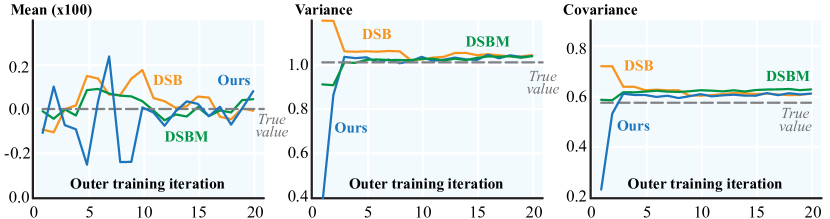
We demonstrate the flexibility of our method on a number of conditional sampling tasks. We first show numerical convergence against the solution of the mirror Schrödinger bridge in a case where an analytical solution is available. Next, we consider resampling from -dimensional datasets and demonstrate control over the in-distribution variation of new data points, which is an added feature of our method. Lastly, we provide examples of image resampling, illustrating how our method can be used to produce image variations with control over the proximity to the original.
5.1 Gaussian Transport
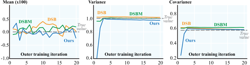
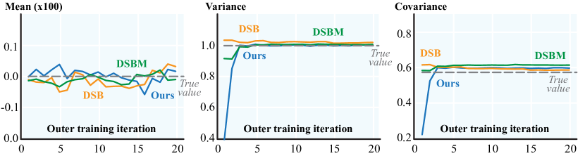
We start by comparing our method with two alternative algorithms, DSB (De Bortoli et al., 2021) and DSBM (Shi et al., 2023), when applied to the mirror Schrödinger bridge case on Gaussians of varying dimension. Figure 1 shows that, in the case of dimension , as the number of outer iterations increases, the empirical convergence of our method performs on par with both DSB and DSBM with the added benefit that each outer iteration with our algorithm requires half the training iterations. Recall that our method trains a single neural network to model a time-symmetrized drift function rather than a neural network for each of the forward and backward drift functions. More details on the derivation of the analytical solution for this experiment, as well as information on parameters, can be found in Appendix B. Additional results for dimensions can be found in Figure 6.
5.2 2D Datasets
To illustrate the behavior of our method, we use our algorithm to resample from 2-dimensional distributions. Unlike the mirror Schrödinger bridge with Gaussians, an analytical solution for mirror bridge with these more general distributions is not known. We consider learning the drift function associated with the mirror Schrödinger bridge that flows samples from to itself. The goal is to obtain new samples that are in the distribution but exhibit some level of variation, i.e., in-distribution variation, correlated to the noise coefficient in the diffusion process. Note that computing mirror Schrödinger bridges with a range of noise values by training one neural network is not possible using existing alternative methods.
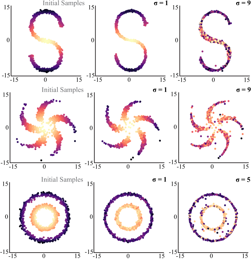
In the columns of Figure 2, we show the result of flowing samples via the mirror Schrödinger bridge with varying values of noise. We observe that the in-distribution variation of data points is controlled by the choice of value, which can indeed be detected by the mixing of colors, or lack of thereof, in each terminal distribution shown. For instance, in the bottom row, we find mixing from samples between the inner and outer circles with the largest value of , compared with no mixing of samples between circles with the smallest value of sigma.
5.3 Image Resampling
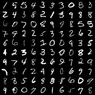
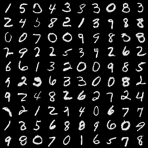
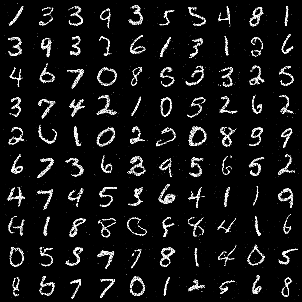
We also train our algorithm on each of the MNIST, CelebA, and Flower datasets. Details on training parameters and architecture for all experiments using images can be found in Appendix C. Our results show that mirror Schrödinger bridges can be used to produce new samples from an image dataset with control over the proximity to the initial sample. In Figure 3, we resample from MNIST using varying levels of noise. We find that pushforward images obtained with a lower fixed value of noise (3(b)) are visually closer to the initial images (3(a)) obtained with a higher fixed value of noise (3(c)).
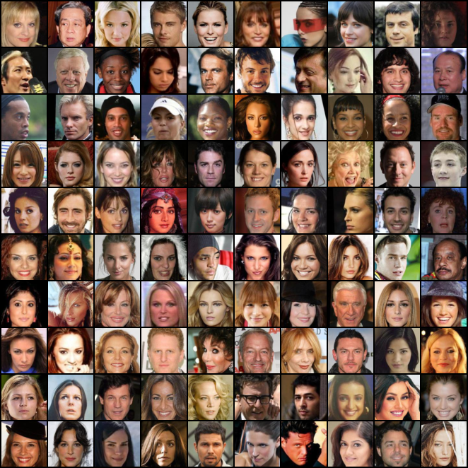
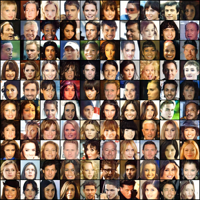
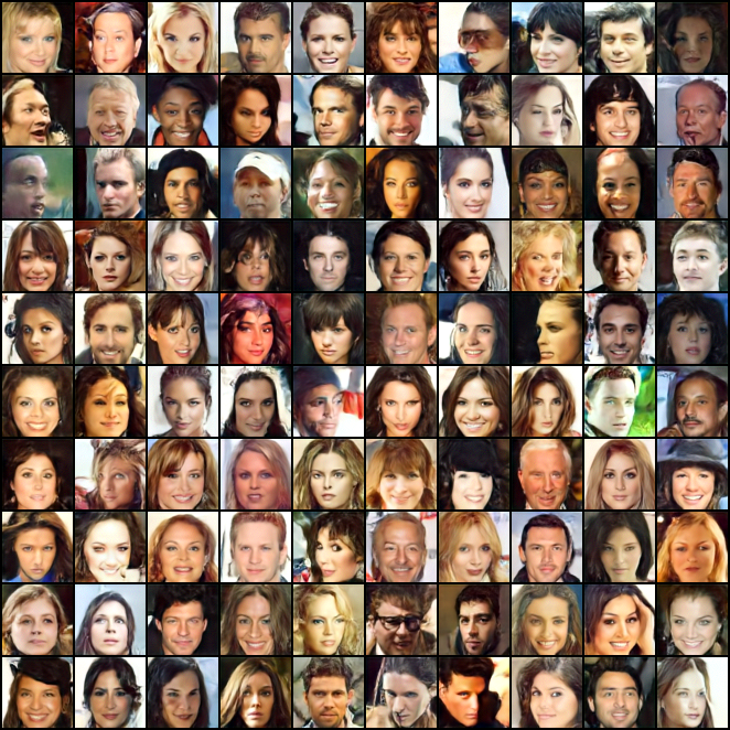
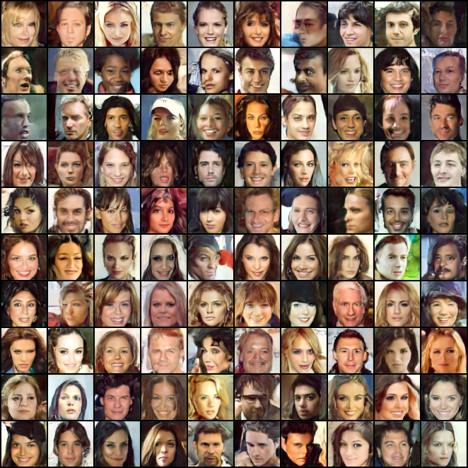
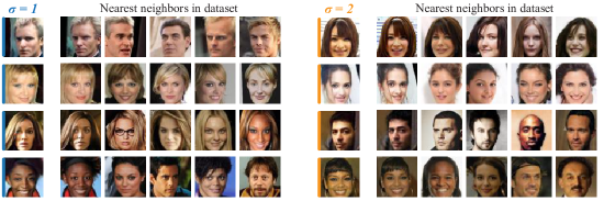
Figure 4 demonstrates the same control over the in-distribution variation of pushforward samples using the RGB dataset CelebA. In each column, we exhibit a different sample from the dataset and, from top to bottom, we show the pushforward samples obtained with varying levels of noise. Across a fixed column, all images resemble the initial sample to varying degrees. In particular, note that the images on the bottom are the least similar to the initial sample, whereas the images on the second row are the most proximal. Images across rows were obtained without retraining the network. This can be done as long as the values chosen for the noise are within the range of values on which the network was trained. Figure 8 includes more results using the CelebA dataset, and Figure 7 shows the nearest neighbors in the dataset to the generated images. In the latter Figure, as desired, the nearest neighbor of the generated sample is the initial sample itself, and the generated sample is distinct from all of its nearest neighbors, showing that our model does not simply regurgitate nearest neighbors of the initial sample as proximal outputs.
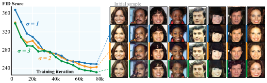
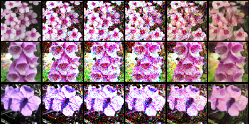
Figure 5 highlights how mirror Schrödinger bridges can be used as a flexible and well-principled tool to perform small edits to RGB images while guaranteeing the result to be in-distribution. This task can be performed by choosing an appropriately small value for .
6 Conclusion
By studying an overlooked version of the Schrödinger bridge problem, which we coin the mirror Schrödinger bridge, we present an algorithm to sample with control over the in-distribution variation of new data points. Our method is flexible and requires fewer training iterations than existing alternatives (De Bortoli et al., 2021; Shi et al., 2023) designed for the general Schrödinger bridge problem. From a theoretical perspective, our method presents advantages over mirror interpolants (Albergo et al., 2023), specifically by obtaining kinetic optimality. While one might consider optimizing fixed mirror interpolants, the resulting - optimization problem is intractable (Shaul et al., 2023). By contrast, our method is numerically tractable, is well-principled, and cuts down training in applications where control over in-distribution variation is desired. On the application front, we demonstrate that our method is a flexible tool to obtain new data points from empirical distributions in a variety of domains, including -dimensional measures and image datasets.
Acknowledgments
The authors would like to thank Lingxiao Li, Artem Lukoianov and Christopher Scarvelis for discussion and feedback. We are also grateful to Suvrit Sra and Francisco Vargas for thoughtful insights on related work. We thank Ahmed Mahmoud for proofreading. Leticia Mattos Da Silva acknowledges the generous support of a MathWorks Engineering Fellowship. Silvia Sellán is supported by an MIT Postdoctoral Fellowship for Engineering Excellence. The MIT Geometric Data Processing Group acknowledges the generous support of Army Research Office grants W911NF2010168 and W911NF2110293, of National Science Foundation grant IIS-2335492, from the CSAIL Future of Data program, from the MIT–IBM Watson AI Laboratory, from the Toyota–CSAIL Joint Research Center, and from the Wistron Corporation.
References
- Agarwal et al. (2024) Medha Agarwal, Zaid Harchaoui, Garrett Mulcahy, and Soumik Pal. Iterated Schrödinger bridge approximation to Wasserstein gradient flows, 2024. URL https://arxiv.org/abs/2406.10823.
- Albergo et al. (2023) Michael S. Albergo, Nicholas M. Boffi, and Eric Vanden-Eijnden. Stochastic interpolants: A unifying framework for flows and diffusions, 2023. URL https://arxiv.org/abs/2303.08797.
- Brekelmans & Neklyudov (2023) Rob Brekelmans and Kirill Neklyudov. On Schrödinger bridge matching and expectation maximization. In NeurIPS 2023 Workshop Optimal Transport and Machine Learning, 2023. URL https://openreview.net/forum?id=Bd4DTPzOGO.
- Chen et al. (2016) Yongxin Chen, Tryphon T. Georgiou, and Michele Pavon. On the relation between optimal transport and Schrödinger bridges: a stochastic control viewpoint. J. Optim. Theory Appl., 169(2):671–691, 2016. ISSN 0022-3239,1573-2878. doi: 10.1007/s10957-015-0803-z. URL https://doi.org/10.1007/s10957-015-0803-z.
- Courty et al. (2017) Nicolas Courty, Rémi Flamary, Devis Tuia, and Alain Rakotomamonjy. Optimal transport for domain adaptation. IEEE Trans. Pattern Anal. Mach. Intell., 39(9):1853–1865, sep 2017. ISSN 0162-8828.
- Csiszár & Matus (2003) Imre Csiszár and Frantisek Matus. Information projections revisited. IEEE Transactions on Information Theory, 49(6):1474–1490, 2003. doi: 10.1109/TIT.2003.810633.
- Csiszár & Tusnády (1984) Imre Csiszár and Gábor Tusnády. Information geometry and alternating minimization procedures. pp. 205–237. 1984. Recent results in estimation theory and related topics.
- Cuturi (2013) Marco Cuturi. Sinkhorn distances: Lightspeed computation of optimal transport. In C.J. Burges, L. Bottou, M. Welling, Z. Ghahramani, and K.Q. Weinberger (eds.), Advances in Neural Information Processing Systems, volume 26. Curran Associates, Inc., 2013. URL https://proceedings.neurips.cc/paper_files/paper/2013/file/af21d0c97db2e27e13572cbf59eb343d-Paper.pdf.
- De Bortoli et al. (2021) Valentin De Bortoli, James Thornton, Jeremy Heng, and Arnaud Doucet. Diffusion Schrödinger bridge with applications to score-based generative modeling. In A. Beygelzimer, Y. Dauphin, P. Liang, and J. Wortman Vaughan (eds.), Advances in Neural Information Processing Systems, 2021. URL https://openreview.net/forum?id=9BnCwiXB0ty.
- Deming & Stephan (1940) W. Edwards Deming and Frederick F. Stephan. On a Least Squares Adjustment of a Sampled Frequency Table When the Expected Marginal Totals are Known. The Annals of Mathematical Statistics, 11(4):427 – 444, 1940. doi: 10.1214/aoms/1177731829. URL https://doi.org/10.1214/aoms/1177731829.
- Essid & Pavon (2019) Montacer Essid and Michele Pavon. Traversing the Schrödinger bridge strait: Robert Fortet’s marvelous proof redux. J. Optim. Theory Appl., 181(1):23–60, 2019. ISSN 0022-3239,1573-2878. doi: 10.1007/s10957-018-1436-9. URL https://doi.org/10.1007/s10957-018-1436-9.
- Feydy et al. (2019) Jean Feydy, Thibault Séjourné, François-Xavier Vialard, Shun-ichi Amari, Alain Trouvé, and Gabriel Peyré. Interpolating between optimal transport and mmd using sinkhorn divergences. In The 22nd International Conference on Artificial Intelligence and Statistics, pp. 2681–2690. PMLR, 2019.
- Fortet (1940) Robert Fortet. Résolution d’un système d’équations de M. Schrödinger. J. Math. Pures Appl. (9), 19:83–105, 1940. ISSN 0021-7824.
- He et al. (2016) Kaiming He, Xiangyu Zhang, Shaoqing Ren, and Jian Sun. Deep residual learning for image recognition. In Proceedings of the IEEE conference on computer vision and pattern recognition, pp. 770–778, 2016.
- Ho et al. (2020) Jonathan Ho, Ajay Jain, and Pieter Abbeel. Denoising diffusion probabilistic models. In H. Larochelle, M. Ranzato, R. Hadsell, M.F. Balcan, and H. Lin (eds.), Advances in Neural Information Processing Systems, volume 33, pp. 6840–6851. Curran Associates, Inc., 2020. URL https://proceedings.neurips.cc/paper_files/paper/2020/file/4c5bcfec8584af0d967f1ab10179ca4b-Paper.pdf.
- Jamison (1975) Benton Jamison. The Markov processes of Schrödinger. Z. Wahrscheinlichkeitstheorie und Verw. Gebiete, 32(4):323–331, 1975. doi: 10.1007/BF00535844. URL https://doi.org/10.1007/BF00535844.
- Kuhn (1955) Harold W. Kuhn. The Hungarian method for the assignment problem. Naval Research Logistics Quarterly, 2(1-2):83–97, 1955.
- Kullback (1968) Solomon Kullback. Probability Densities with Given Marginals. The Annals of Mathematical Statistics, 39(4):1236 – 1243, 1968.
- Kurras (2015) Sven Kurras. Symmetric Iterative Proportional Fitting. In Guy Lebanon and S. V. N. Vishwanathan (eds.), Proceedings of the Eighteenth International Conference on Artificial Intelligence and Statistics, volume 38 of Proceedings of Machine Learning Research, pp. 526–534, San Diego, California, USA, 09–12 May 2015. PMLR.
- Léonard (2014) Christian Léonard. Some Properties of Path Measures, pp. 207–230. Springer International Publishing, Cham, 2014. ISBN 978-3-319-11970-0. doi: 10.1007/978-3-319-11970-0˙8. URL https://doi.org/10.1007/978-3-319-11970-0_8.
- Léonard (2014) Christian Léonard. A survey of the Schrödinger problem and some of its connections with optimal transport. Discrete Contin. Dyn. Syst., 34(4):1533–1574, 2014. ISSN 1078-0947,1553-5231. doi: 10.3934/dcds.2014.34.1533. URL https://doi.org/10.3934/dcds.2014.34.1533.
- Mensch et al. (2019) Arthur Mensch, Mathieu Blondel, and Gabriel Peyré. Geometric losses for distributional learning. In International Conference on Machine Learning, pp. 4516–4525. PMLR, 2019.
- Peluchetti (2023) Stefano Peluchetti. Diffusion bridge mixture transports, Schrödinger bridge problems and generative modeling. Journal of Machine Learning Research, 24(374):1–51, 2023. URL http://jmlr.org/papers/v24/23-0527.html.
- Ruschendorf (1995) Ludger Ruschendorf. Convergence of the Iterative Proportional Fitting Procedure. The Annals of Statistics, 23(4):1160 – 1174, 1995.
- Sander et al. (2022) Michael E. Sander, Pierre Ablin, Mathieu Blondel, and Gabriel Peyré. Sinkformers: Transformers with doubly stochastic attention. In Gustau Camps-Valls, Francisco J. R. Ruiz, and Isabel Valera (eds.), International Conference on Artificial Intelligence and Statistics, AISTATS 2022, 28-30 March 2022, Virtual Event, volume 151 of Proceedings of Machine Learning Research, pp. 3515–3530. PMLR, 2022. URL https://proceedings.mlr.press/v151/sander22a.html.
- Schrödinger (1932) Erwin Schrödinger. Sur la théorie relativiste de l’électron et l’interprétation de la mécanique quantique. Annales de l’institut Henri Poincaré, 3:269–310, 1932. URL http://dml.mathdoc.fr/item/AIHP_1932__2_4_269_0.
- Shaul et al. (2023) Neta Shaul, Ricky T. Q. Chen, Maximilian Nickel, Matt Le, and Yaron Lipman. On kinetic optimal probability paths for generative models. In Proceedings of the 40th International Conference on Machine Learning, ICML’23. JMLR.org, 2023.
- Shi et al. (2022) Yuyang Shi, Valentin De Bortoli, George Deligiannidis, and Arnaud Doucet. Conditional simulation using diffusion Schrödinger bridges. In James Cussens and Kun Zhang (eds.), Proceedings of the Thirty-Eighth Conference on Uncertainty in Artificial Intelligence, volume 180 of Proceedings of Machine Learning Research, pp. 1792–1802. PMLR, 01–05 Aug 2022. URL https://proceedings.mlr.press/v180/shi22a.html.
- Shi et al. (2023) Yuyang Shi, Valentin De Bortoli, Andrew Campbell, and Arnaud Doucet. Diffusion Schrödinger bridge matching. In Thirty-seventh Conference on Neural Information Processing Systems, 2023. URL https://openreview.net/forum?id=qy07OHsJT5.
- Sinkhorn (1964) Richard Sinkhorn. A relationship between arbitrary positive matrices and doubly stochastic matrices. Annals of Mathematical Statistics, 35:876–879, 1964.
- Song & Ermon (2019) Yang Song and Stefano Ermon. Generative modeling by estimating gradients of the data distribution. In H. Wallach, H. Larochelle, A. Beygelzimer, F. d'Alché-Buc, E. Fox, and R. Garnett (eds.), Advances in Neural Information Processing Systems, volume 32. Curran Associates, Inc., 2019. URL https://proceedings.neurips.cc/paper_files/paper/2019/file/3001ef257407d5a371a96dcd947c7d93-Paper.pdf.
- Song et al. (2021) Yang Song, Jascha Sohl-Dickstein, Diederik P Kingma, Abhishek Kumar, Stefano Ermon, and Ben Poole. Score-based generative modeling through stochastic differential equations. In International Conference on Learning Representations, 2021. URL https://openreview.net/forum?id=PxTIG12RRHS.
- Trajanovski et al. (2023) Pece Trajanovski, Petar Jolakoski, Kiril Zelenkovski, Alexander Iomin, Ljupco Kocarev, and Trifce Sandev. Ornstein-Uhlenbeck process and generalizations: particle dynamics under comb constraints and stochastic resetting. Phys. Rev. E, 107(5):Paper No. 054129, 18, 2023. ISSN 2470-0045,2470-0053. doi: 10.1103/physreve.107.054129. URL https://doi.org/10.1103/physreve.107.054129.
- Vargas & Nüsken (2023) Francisco Vargas and Nikolas Nüsken. Transport, VI, and diffusions. In ICML Workshop on New Frontiers in Learning, Control, and Dynamical Systems, 2023. URL https://openreview.net/forum?id=Ay1b1W7Mjy.
- Vargas et al. (2021) Francisco Vargas, Pierre Thodoroff, Austen Lamacraft, and Neil Lawrence. Solving Schrödinger bridges via maximum likelihood. Entropy, 23(9), 2021.
- Vaswani et al. (2017) Ashish Vaswani, Noam Shazeer, Niki Parmar, Jakob Uszkoreit, Llion Jones, Aidan N Gomez, Ł ukasz Kaiser, and Illia Polosukhin. Attention is all you need. In I. Guyon, U. Von Luxburg, S. Bengio, H. Wallach, R. Fergus, S. Vishwanathan, and R. Garnett (eds.), Advances in Neural Information Processing Systems, volume 30. Curran Associates, Inc., 2017.
- Weis (2014) Stephan Weis. Information topologies on non-commutative state spaces. J. Convex Anal., 21(2):339–399, 2014. ISSN 0944-6532,2363-6394.
- Winkler et al. (2023) Ludwig Winkler, Cesar Ojeda, and Manfred Opper. A score-based approach for training schrödinger bridges for data modelling. Entropy, 25(2), 2023. ISSN 1099-4300. doi: 10.3390/e25020316. URL https://www.mdpi.com/1099-4300/25/2/316.
- Zhou et al. (2024) Linqi Zhou, Aaron Lou, Samar Khanna, and Stefano Ermon. Denoising diffusion bridge models. In The Twelfth International Conference on Learning Representations, 2024. URL https://openreview.net/forum?id=FKksTayvGo.
Appendix A Proof of Proposition 3
The first claimed expression is the very definition of . As for the second claimed expression, let be the sequence of IPFP iterates. Note that by Lemma 2, we have
Since belongs to both projection sets, the Pythagorean theorem for reverse projections (Brekelmans & Neklyudov, 2023, Theorem 3.4) (see also (Csiszár & Matus, 2003, Theorem 5)) yields that for each we have
| (13) |
Now the sequence converges to zero because the sequence converges to zero (see, e.g., (Weis, 2014, Theorem 3.21.4)). Thus, taking the limit as , we deduce that
Now, write . A similar argument shows that
where the last inequality above follows from the nonnegativity of the KL divergence. It follows that also achieves the desired minimum , i.e., we have . Finally, we must rule out the possibility that this minimizer is not unique. To do this, observe that, by the squeeze theorem, we must have
We can now apply Pinsker’s Inequality, which tells us that the KL divergence is at least a constant multiple of the square of the metric induced by total variation. More precisely,we have that . We deduce that
which implies that converges to in total variation. We conclude that . ∎
Appendix B Analytical Solution for Gaussian Experiment
Proposition 4.
Consider the static Schrödinger bridge problem with initial and final marginals equal to the -dimensional Gaussian distribution with zero mean and unit variance, where we take the reference measure corresponding to the OU process running from to . The solution to this problem is a -dimensional Gaussian with zero mean and covariance matrix given by
Proof.
We follow the proof of (De Bortoli et al., 2021, Proposition 46), which established the corresponding result in the case where the reference process has zero drift. Imitating the proof of (De Bortoli et al., 2021, Proposition 43), we see that the static Schrödinger bridge exists and is a -dimensional Gaussian. That the mean equals zero follows from the fact that both marginals have zero mean. The rest of the proof is devoted to determining the covariance matrix of .
The fact that marginals have unit variance implies that . To compute and , we start by computing the probability density function (PDF) of the reference measure , where . Recall that is the product of the conditional PDF of with the PDF of . Thus, we have
Note that has zero mean and unit variance, so up to normalization we have
On the other hand, the mean and variance of the conditional distribution are computed in (Trajanovski et al., 2023, section II), where it is shown that they are respectively given by
It follows that
Combining these calculations, we conclude that the joint distribution has PDF given by
This distribution is evidently a Gaussian with zero mean and covariance matrix given by
Note in particular that the variance of the marginal of at is equal to the coefficient of the bottom-right entry of , which is . Now, the KL divergence between a -dimensional Gaussian distribution with zero mean and covariance matrix and the distribution is given explicitly by
If we take to be of the form
which matches the form of the covariance for , then
where is a nonzero constant independent of . As argued in (De Bortoli et al., 2021, proof of Proposition 46), we can assume is a symmetric matrix, as doing so will only decrease , so is diagonalizable. Let denote the eigenvalues of , counted with multiplicity. Using the well-known formula for the determinant of a block matrix, we find that
Thus, we obtain
Note in particular that since is a covariance matrix, it is positive semi-definite, and so its eigenvalues must be nonnegative, implying that for each .
Minimizing then amounts to take in such a way that is minimized. Observe that the equation
is solved by
We then choose the sign to be to ensure that . ∎
Appendix C Implementation Details
In this section we give further details on our experimental setup.
C.1 Gaussian Transport
We use the MLP large network from (De Bortoli et al., 2021) for DSB and DSBM in all Gaussian transport experiments. For our method, we modify this network to take as an input. The values of are uniformly sampled from the (inclusive) interval from to for training, and at test time we fix for all samples to compare with DSB and DSBM, which do not take as a network input, but each use via the SDE discretization. We run the same experiment for dimension and (in Figure 6), and (in Figure 1). The number of samples for all experiments is . We use timesteps and train for inner iterations for each of outer iterations.
C.2 2D Datasets
We modify the network architecture with positional encoding from (Vaswani et al., 2017), which is used by De Bortoli et al. (2021), to take values of noise rather than tuples of only and . The values of are concatenated to the spatial features before the first MLP block is applied. This modified network is used to parametrize our drift function. We use Adam optimizer with learning rate and momentum . We train each example for inner iterations per outer iteration of the algorithm. Figure 2 shows the terminal samples obtained for outer iteration for all example datasets. The noise values are sampled uniformly in the range from to for training. At test time, a fixed value is chosen for all sample trajectories. We train with samples, which are refreshed each iterations. We use timesteps of size each. All -dimensional experiments run on CPU.
C.3 Image Resampling
For the image dataset experiments, we modify the U-Net architecture used in (De Bortoli et al., 2021; Shi et al., 2023) to take values of noise . Each value is expanded to match image size and concatenated to channels of their corresponding sample image before the input block is applied. For all image experiments we follow the timestep schedule used in De Bortoli et al. (2021) with and . We use Adam optimizer with learning rate and momentum . Experiments with image datasets were run on limited shared GPU resources; lower-resolution image sizes and number of samples in cache were chosen accordingly.
MNIST. For the experiment in Figure 3, we use cached images of size ; the batch size is and the number of timesteps is . The noise values are sampled uniformly in the interval from to (inclusive) during training. We train for iterations per outer iterations, and cached samples are refreshed every inner iterations. The terminal samples shown are for outer iteration .
CelebA. In Figures 4 and 8, we use cached images of size and batch size . The cache is refreshed every inner iterations and we train for iterations per outer iterations. The number of timesteps is ; the values are uniformly sampled in the interval from to . The terminal sample images are shown for outer iteration . The FID score in Figure 4 is computed using images.
Flowers102. For Figure 5, we use cached images of size . The batch size is and cache is refreshed every inner iterations. We train for inner iterations per outer iteration. Terminal samples are shown for outer iteration . The values are uniformly sampled in the interval from to ; the number of timesteps is .
Appendix D Additional Experimental Results