$\beta$-calibration of Language Model Confidence Scores
for Generative QA

Abstract

To use generative question-and-answering (QA) systems for decision-making and in any critical application, these systems need to provide well-calibrated confidence scores that reflect the correctness of their answers. Existing calibration methods aim to ensure that the confidence score is on average indicative of the likelihood that the answer is correct. We argue, however, that this standard (average-case) notion of calibration is difficult to interpret for decision-making in generative QA. To address this, we generalize the standard notion of average calibration and introduce $\beta$-calibration, which ensures calibration holds across different question-and-answer groups. We then propose discretized posthoc calibration schemes for achieving $\beta$-calibration.

Keywords: calibration; question-answering

1 Introduction

Language models (LMs) built on transformer-based architectures are capable of producing texts that are both coherent and contextually relevant for a large range of applications (Brown et al., 2020; Chowdhery et al., 2023; Achiam et al., 2023). In question-and-answering (QA) systems, these models generally perform well, but occasionally produce inaccurate answers – a phenomenon generally referred to as hallucination (Huang et al., 2023). Confidence estimates that are paired with the answers can be used as an interpretable indicator of the LM’s accuracy (Steyvers et al., 2024). But for this, these confidence scores have to be well-calibrated, i.e., match the actual accuracy of the model.

To evaluate whether the obtained confidence scores are actually well-calibrated, a common criterion is the expected (average-case) calibration error (Tian et al., 2023; Xiong et al., 2024). Suppose a model claims that its answer has a confidence of $p$. Based on only this one answer it is not possible to know whether this confidence was well-calibrated or not. But when considering multiple question-answer pairs, let’s say $N_{p}$ with claimed confidence $p$, we can verify how many answers were actually correct and measure the error between the claimed confidence and the model’s accuracy. By averaging over all these errors, we can measure the calibration of the model’s confidence scores.

While this average-case calibration measure makes sense for models trained and evaluated on specific tasks, its applicability for generative QA is highly questionable due to the averaging is now over all QA pairs. The reason being that generative QA systems can be applied in various domains and topics, e.g., to answer questions about geography as well as about politics or medicine. Consider, for instance, the QA pairs shown in Figure 1. On average this model has a calibration error of $0.5$. But as far as User 1 is concerned, the calibration is much worse with an error of $0.8$. User 2, on the other hand, makes a completely different experience, as for them the model seems to be much better calibrated than indicated by the average calibration error. This motivates our notion of $\beta$-calibration, where the calibration target is conditional on the group of the question-and-answer pair.

Previous works have explored group-wise calibration for classifiers, using pre-specified groupings of their covariates (e.g., race or gender) (Kleinberg et al., 2017; Pleiss et al., 2017). However, it is not clear how this idea can be transplanted to the generative QA setting.

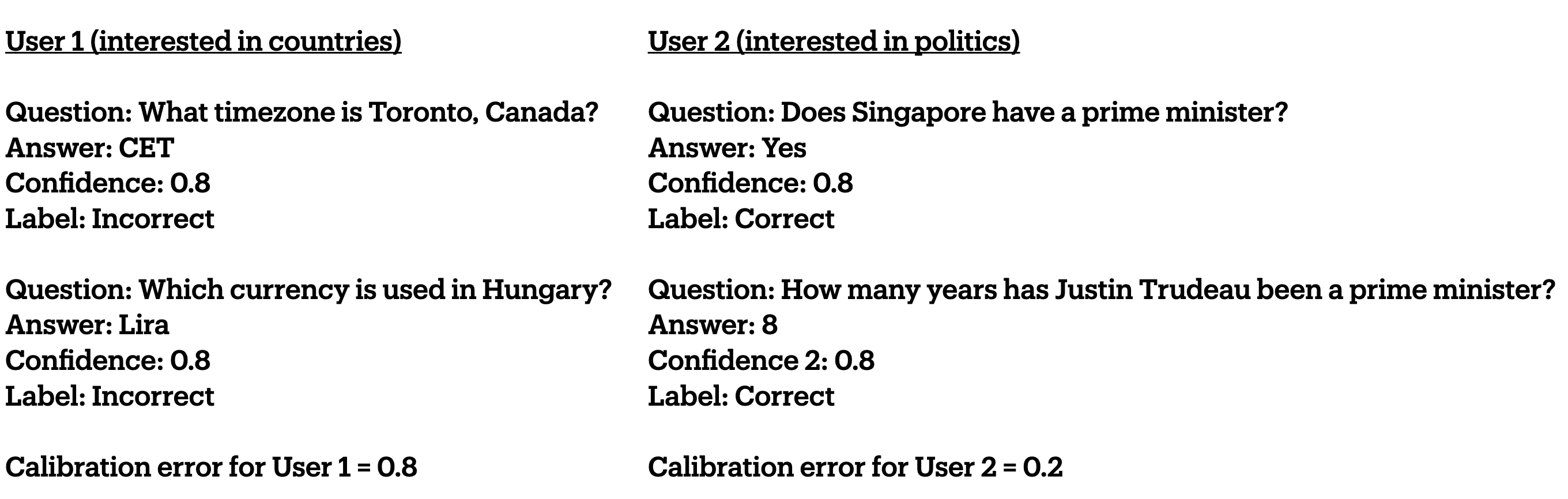
Figure 1: Two users interact separately with an LM by inputting questions and obtaining answers and confidence scores from the LM. The LM could be calibrated on average across user types, but each individual user may not have calibrated confidence scores. See Example 2.1 for more details.

A common approach to obtain calibrated confidence scores in LMs is to use confidence elicitation via prompting (Tian et al., 2023; Xiong et al., 2024). The advantage of this approach is that it can be executed with only black-box access to LMs. However, the issue with a pure elicitation via prompting approach is that the performance is sensitive to choice of prompts and model (Sclar et al., 2024), and it does not have any rigorous calibration guarantees. These issues can be mitigated by performing a posthoc calibration of the elicited confidence scores. Our proposed approach is such a posthoc calibration method.

A limitation of relying on LM-elicited confidence directly, or post-hoc calibrated using temperature scaling  (Tian et al., 2023), is that the output probability is not discretized, making performance difficult to assess  (Kumar et al., 2019). We overcome this problem by developing posthoc $\beta$-calibration schemes on elicited confidence scores that use ideas of (histogram) binning (Zadrozny and Elkan, 2001) and scaling-binning (Kumar et al., 2019) that are by construction discretized.

Our Contributions: We make the following contributions in this paper:

1. We define $\beta$-calibration, a principled and interpretable notion of calibration in the generative QA setting. The $\beta$ here refers to any fixed mapping of all possible question-and-answer pairs to a finite set. Our $\beta$-calibration notion generalizes the standard average-case calibration notion by requiring calibration conditional on $\beta$. Due to this conditioning on $\beta$, the guarantee of $\beta$-calibration is stronger than the standard calibration guarantee. By instantiating this framework with different $\beta$’s, we have the flexibility of defining question-and-answer groups across which we would like calibration guarantees to hold. In this paper, we present an instantiation of $\beta$ as a kd-tree, an adaptive multivariate histogram method that provides cohesive groupings of QA pairs.

2. We propose two posthoc calibration techniques for $\beta$-calibration: (a) $\beta$-binning and (b) scaling-$\beta$-binning. The latter uses the former as a subroutine. This is particularly useful in the practical setting where some $\beta$-induced groups may lack data. We show that both methods satisfy a distribution-free approximate $\beta$-calibration guarantee. In both cases, the approximation level is used to decide on the number of points per bin, a key hyperparameter.

3. Finally, we experiment on newly developed elicitation prompts across 5 commonly used QA benchmark datasets of various sizes. We find that $\beta$-binning and scaling-$\beta$-binning achieve lower $\beta$-calibration error than elicited confidence scores and other baselines. We further justify our framework by demonstrating its performance in a downstream selective QA task. Our posthoc calibration algorithms achieve around 10-40% increase in $\beta$-calibration performance and up to 30% increase in selective answering performance.

2 Defining $\beta$-Calibration

2.1 Notation

We first define the question-and-answering process with verbalized confidence elicitation. In the most minimal form of interaction, a question $q$, is embedded into a prompt using a prompt function $m(q)$. The user obtains an answer $a=c(m(q))$ from an answering function $c:{\mathcal{Q}}\rightarrow{\mathcal{A}}$. Note that $c$ could be a randomized function, as typical LMs are. Confidence elicitation (Xiong et al., 2024; Tian et al., 2023) enhances the prompt to let the user obtain confidence $h(m(q),a)$ from the confidence function $h:{\mathcal{Q}}\times{\mathcal{A}}\rightarrow[0,1]$. Note that both answering and confidence functions are implicit in the LM interaction. In the following, for simplicity, we omit the dependence on prompt function $m$, and use $c(q)$ for $c(m(q))$ and $h(q,a)$ for $h(m(q),a)$. We assume that we have access to the binary ground truth $y$ for each pair $(q,a)$, which indicates whether the answer $a$ is correct ($y=1$) for the question $q$. Our $N$-element dataset is then $D=\{(q_{i},a_{i},h_{i},y_{i})\}_{i\in[N]}$ where $q_{i}$ is the $i$th question, $a_{i}=c(q_{i})$, $h_{i}=h(q_{i},a_{i})$ and $y_{i}$ is the label which indicates whether the answer $a_{i}$ is correct for the question $q_{i}$. For more details, refer to Table 3. We assume that each instance $(q,a,h,y)$ of $D$ is an i.i.d. realization of r.v. $(Q,A=c(Q),H=h(Q,A),Y)$ drawn from a fixed distribution $P$ over the ${\mathcal{Q}}\times{\mathcal{A}}\times[0,1]\times[0,1]$ where

$$P:=P_{Q}\times P_{A|q}\times P_{H|q,a}\times P_{Y|q,a}\leavevmode\nobreak\ .$$ (1)

Definition 2.1 (Calibration).

We say that $h$ is calibrated for distribution $P$ if:

$$\mathbb{E}\left[Y\mid h(Q,A)=p\right]=p,\mbox{ a.s. for all $p\in[0,1]$}$$ (2)

In words, that the conditional distribution on $Y$ conditional on the prediction that $h(Q,A)=p$ is a Bernoulli distribution with bias $p$. In the following, we refer to Eq. ( 2) as average-case calibration to distinguish it from $\beta$-calibration.

While perfect calibration is impossible in finite samples, a standard measure for calibration error of $h$ is defined as follows.

Definition 2.2 (Expected (Average-case) Calibration Error).

The expected (average-case) calibration error of $h$ is defined as:

$$\text{CE}(h)=\mathbb{E}_{Q,A}\left[\left|\mathbb{E}[Y\mid h(Q,A)]-h(Q,A)\right|\right]$$ (3)

2.2 $\beta$-calibration Instead of Standard Calibration

In practice, a user who obtains an answer $a$ to their question $q$ with confidence $p$ wants to know the probability that $y=1$ among “similar” $(q,a)$ pairs with confidence $p$ (e.g., within the same topic of interest). A perfectly calibrated $h$ however, may not satisfy this requirement, as we illustrate in the following example:

Example 2.1.

Suppose the dataset consists of two sets of QA pairs, $\beta_{1}=\{(q_{11},a_{11}),(q_{12},a_{12})\}$, and $\beta_{2}=\{(q_{21},a_{21}),(q_{22},a_{22})\}$ with confidence function $h$ and $\mathbb{P}(Y=1|q,a)$ as shown in Table 1.

Table 1: QA pairs with confidence and correctness for Example 2.1.

Question $q$	Answer $a$	Confidence $h(q,a)$	$\mathbb{P}(Y=1|q,a)$
$q_{11}$	$a_{11}$	0.8	0.6
$q_{12}$	$a_{12}$	0.8	0.7
$q_{21}$	$a_{21}$	0.8	0.9
$q_{22}$	$a_{22}$	0.8	1.0

It can easily be seen that $h$ is perfectly calibrated according to Eq. ( 2) when we assume that each QA pair have the same sampling probability. However, when we consider the sets $\beta_{1}$ and $\beta_{2}$ separately, each set is not well-calibrated.

$$\mathbb{E}[Y|h(q,a)=0.8,\beta_{1}]=\frac{1}{2}({\mathbb{P}}[Y=1\mid q_{11},a_{11}]+{\mathbb{P}}[Y=1\mid q_{12},a_{12}])=\frac{1}{2}(0.6+0.7)=0.65,$$

$$\mathbb{E}[Y|h(q,a)=0.8,\beta_{2}]=\frac{1}{2}({\mathbb{P}}[Y=1\mid q_{21},a_{21}]+{\mathbb{P}}[Y=1\mid q_{22},a_{22}])=\frac{1}{2}(0.9+1.0)=0.95.$$

Practically, when a user is only concerned with a particular set $\beta_{1}$ or $\beta_{2}$, the calibration claim does not align with reality. For $\beta_{1}$, $h$ is overconfident, and underconfident for $\beta_{2}$.

In the above, the expectation $\mathbb{E}[Y\mid h(q,a)]$ is not interpretable from a decision-making perspective. The space of generative QA pairs ${\mathcal{Q}}\times{\mathcal{A}}$ is intuitively too large for a user, particularly since they are typically only interested in a smaller subset of $(q,a)$ pairs. We hence consider a generalization of Eq. ( 2) necessary to perform adequate calibration for generative QA.

Definition 2.3.

($\beta$-calibration) $h$ is $\beta$-calibrated for the distribution $P$ in Eq. ( 1) if:

$$\mathbb{E}\left[Y\mid h(Q,A)=p,\beta(Q,A)\right]=p,$$ (4)

a.s. for all $p\in[0,1]$, where $\beta:{\mathcal{Q}}\times{\mathcal{A}}\rightarrow{\mathcal{S}}$ for some embedding space ${\mathcal{S}}$.

In this work, we focus on a finite set ${\mathcal{S}}$ and $\beta$ is a (deterministic) discretization scheme that maps $(q,a)$ to a finite set $S$, i.e., $\beta$ induces a partitioning of the QA space according to the output of $\beta$. Note that this $\beta$-calibration reduces to calibration in Eq. ( 2) if $\beta(q,a)$ is the same for all question-and-answers $(q,a)$. Intuitively, $\beta$ is chosen such that the pre-image of a specific value of $\beta$ represents a grouping that an end-user might be interested in.

Going back to Example 2.1, $\beta$-calibration would tell us the following: “among question and answer pairs with confidence $p$ that are mapped to the same $\beta$ value (as the user’s $(q,a)$ pair), the fraction who are correct ($y=1$) is also $p$”. Further, we also extend Eq. ( 3) to propose an error metric for $\beta$-calibration:

Definition 2.4 ($\beta$-calibration error).

The $\beta$-calibration error of $h$ is defined as:

$$\text{CE}(h;\beta)=\mathbb{E}_{Q,A}\left[\left|\mathbb{E}[Y\mid h(Q,A),\beta(Q,A)]-h(Q,A)\right|\right].$$

2.3 Generalizing (Average) Calibration via kd-Tree Instantiation of $\beta$

The definition of $\beta$-calibration (Definition 2.3), requires a predefined $\beta$ mapping. While our schemes developed in Section 3 can work with any arbitrary $\beta$ mapping, we propose a general approach for $\beta$ in the language model QA setting: the embed-then-bin method. This involves computing vector embeddings from question-and-answer pairs and then creating a multidimensional histogram over these embeddings. The range of $\beta$ is then set to index over the histogram bins of the embeddings. We write $\beta=\beta_{\text{hist}}\circ\beta_{\text{emb}}$, where $\beta_{\text{emb}}:{\mathcal{Q}}\times{\mathcal{A}}\rightarrow\mathbb{R}^{M}$ computes an $M$-dimensional embedding and $\beta_{\text{hist}}:{\mathbb{R}}^{M}\rightarrow{\mathcal{S}}$ computes the index of the embedding histogram bin containing the embedding.

Specifically, we use the [CLS] token embedding from the pre-trained DistilBERT model (Sanh et al., 2019): $\beta_{\text{emb}}:{\mathcal{Q}}\times{\mathcal{A}}\rightarrow\mathbb{R}^{768}$ ($M=768$). As for the histogram, we adapt a kd-tree (Bentley, 1975) to bin each vector to an integer representing the index of the partition containing the vector: $\beta_{\text{hist}}:{\mathbb{R}}^{768}\rightarrow S$, where $S$ is the set of partition indices. See Appendix C for details on our kd-tree construction. An important hyperparameter is the maximum depth of the tree $d$, which determines the number of partitions.

While DistilBERT is designed to be smaller and faster than its alternatives, it is still able to generate high-quality contextual embeddings that are rich in semantic information. Next, a kd-tree performs efficient and adaptive binning for the high-dimensional embedding space by successively splitting along different dimensions. Each partition of the tree contains semantically-similar $(q,a)$ pairs that are “near” each other in the embedding space.

The choice of kd-tree generalizes the standard calibration as when $d=0$, $\text{CE}(h;\beta)$ reduces to $\text{CE}(h)$. The hyperparameter $d$ should be chosen based on the downstream metric that needs to be optimized. In the experiments section, we further describe how $\beta_{\text{hist}}$ are constructed.

3 Achieving Posthoc $\beta$-Calibration

As discussed earlier, an elicited confidence score function ($h$) of LM-model is not guaranteed to be $\beta$-calibrated (or even calibrated under average-case). For any $\beta:{\mathcal{Q}}\times{\mathcal{A}}\rightarrow{\mathcal{S}}$, the goal of posthoc $\beta$-calibration is to design a scheme that that can take any $h$ and transform it to a $\beta$-calibrated confidence score. We wish to learn a posthoc calibrator $g:[0,1]\rightarrow[0,1]$ such that $g\circ h$ is (approximately) $\beta$-calibrated using a calibration dataset $D=\{(q_{i},a_{i},h_{i},y_{i})\}_{i\in[N]}$. Additional missing details from this section are collected in Appendix A.

Our recalibration schemes utilize the existing building blocks in posthoc calibration literature, like histogram binning (Zadrozny and Elkan, 2001) and scaling (Platt, 1999). The novelty of our recalibration methods lies how we generalize and combine these building blocks achieving the best of both worlds: our binning component generalizes histogram binning to any partitioning and enables distribution-free guarantees, and our hierarchical scaling component reduces overfitting, enabling learning to be performed across partitions which may have varied number of data points.

Our schemes take the $\beta$ function as input, and all our schemes and theoretical results hold for any $\beta$. In our experiments, we will use the kd-trees based $\beta$ instantiation from Section 2.3. We focus on methods that output discretized scores, since this has been shown to be easier to assess (Appendix A.1). We achieve this by first discretizing the QA space using $\beta$ and then ensuring that for each QA partition $s\in{\mathcal{S}}$ we output a calibrated confidence score. We start by describing an adaptation of the classical histogram binning (Zadrozny and Elkan, 2001) idea for achieving $\beta$-calibration. In Section 3.2, we build upon this to provide a more robust algorithm that also uses S before binning.

3.1 Approach 1: $\beta$-binning

$\beta$-binning is a standalone posthoc $\beta$-calibration algorithm. It uses as a subroutine, uniform-mass-double-dipping histogram binning(UMD) (Gupta and Ramdas, 2021), which we describe in Algorithm 4. Informally, the UMD procedure partitions the interval $[0,1]$ into $B$ bins using the histogram of $h$ values from the calibration dataset $D$, ensuring that each bin has approximately the same number of calibration points. It returns a calibrator function $g_{\text{UMD}}$ that takes as input an uncalibrated confidence score, then allocates it to one of the $B$ bins, and returns the probability of label being $1$ (estimated as the average of the $y$ values from the calibration dataset $D$ that are mapped into that bin).

In Algorithm 1, we present a subroutine that uses the UMD procedure to construct a different calibrator for each QA-partition, which we will invoke with different inputs. Algorithm 1 takes as input a dataset ${\mathcal{D}}=\{\left(q_{i},a_{i},h_{i},t_{i}\right)\}_{i\in[n]}$ where $h_{i}$ is the (elicited) confidence score for the answer $a_{i}$ and $t_{i}$ is the (potentially noisy) label of the correctness of answer $a_{i}$ for the question $q_{i}$. Algorithm 1 partitions the input dataset ${\mathcal{D}}$ to $\{{\mathcal{D}}_{s}\}_{s\in{\mathcal{S}}}$, where ${\mathcal{D}}_{s}=\{\left(q_{i},a_{i},h_{i},t_{i}\right):\beta(q_{i},a_{i})=s\}$. For each $s\in{\mathcal{S}}$, UMD is fit using ${\mathcal{D}}_{s}$ to construct a $g_{\text{UMD}}$ calibrator that is stored in a hash table ${\mathcal{G}}$, keyed by $s$. We next describe the training and test processes of $\beta$-binning.

Algorithm 1 $\beta$-binning: Train-time Subroutine

0:  Calibration data: ${\mathcal{D}}=\{\left(q_{i},a_{i},h_{i},t_{i}\right)\}_{i\in[n]}$. Hyperparameters: Minimum number of points per bin $b\in\mathbb{N}$ (say 50), tie-breaking parameter $\delta>0$ (default: $10^{-10}$)

0:  Hash table ${\mathcal{G}}$ of fitted UMD calibrators $g_{\text{UMD}}$’s, keyed by partition index $s\in{\mathcal{S}}$ /* First construct UMD calibrator for points outside of bounded kd-tree spaces and store in ${\mathcal{G}}$ with a default key, say root*/

1:  $g_{{\mathcal{D}}}\leftarrow\text{UMD}({\mathcal{D}},B=\lfloor|{\mathcal{D}}|/b\rfloor,\delta=\delta)$.

2:  ${\mathcal{G}}[\texttt{root}]\leftarrow g_{{\mathcal{D}}}$

3:  for $s\in{\mathcal{S}}$ do

4:     ${\mathcal{D}}_{s}\leftarrow\left\{(h_{i},t_{i}):\beta(q_{i},a_{i})=s\right\}_{i\in[n]}$

5:     /* If ${\mathcal{D}}_{s}$ is empty then continue to the next $s$ */

6:     $n_{s}\leftarrow\left|{\mathcal{D}}_{s}\right|$

7:     ${\mathcal{G}}[s]\leftarrow\text{UMD}(\mathcal{D}={\mathcal{D}}_{s},B=\lfloor n_{s}/b\rfloor,\delta=\delta)$

8:  end for

9:  return  ${\mathcal{G}}$

Algorithm 2 $\beta$-binning: Test-time Subroutine

0:  Test question, answer and confidence score: $(q_{\text{test}},a_{\text{test}},h_{\text{test}})$, Hash table ${\mathcal{G}}$

0:  (Approximately) $\beta$-calibrated confidence score

1:  if $\beta(q_{\text{test}},a_{\text{test}})\in{\mathcal{G}}$ then

2:     $g_{\text{UMD}}\leftarrow{\mathcal{G}}[\beta(q_{\text{test}},a_{\text{test}})]$

3:     return  $g_{\text{UMD}}(h_{\text{test}})$

4:  else

5:     /* In this case, the test input $(q_{test},a_{test})$ does not lie in any of the bounded kd-tree spaces*/

6:     $g_{{\mathcal{D}}}\leftarrow{\mathcal{G}}[\texttt{root}]$

7:     return  $g_{{\mathcal{D}}}(h_{\text{test}})$

8:  end if

Training Process. We invoke Algorithm 1 on our calibration dataset $D$, i.e., ${\mathcal{D}}=D$. Hence, $t_{i}$ in Algorithm 1 is set to the ground truth $y_{i}$. The output is a hash table of UMD calibrator functions indexed by the entries in the range $S$ of $\beta$.

Test Process. For a test input $(q_{\text{test}},a_{\text{test}},h_{\text{test}})$, we invoke Algorithm 2. A fitted UMD ($g_{\text{UMD}}$) for this $(q_{\text{test}},a_{\text{test}})$ pair is retrieved from the hash table ${\mathcal{G}}$ using $\beta(q,a)$ as key, which is then invoked to obtain a $\beta$-calibrated confidence score $g_{\text{UMD}}(h_{\text{test}})$. In our kd-tree instantation, if ${\mathcal{G}}$ does not have a calibrator for a $\beta(q_{\text{test}},a_{\text{test}})$, we use UMD to calibrate that pair. This corresponds to points that lie outside of the bounded kd-tree spaces (refer to Appendix C). Since we can generate a large amount of question-and-answer pairs without requiring ground truth, the number of test points in our experiments that fall outside the bounded spaces is negligible.

Note that while we assumed here access to the true labels $y_{i}$’s, we can also operate $\beta$-binning with proxy labels generated by say another LM on QA pairs, as discussed more in following subsections. In practice, users are likely to define large $S$ (for example, large maximum depth of tree $d$) in order to obtain more cohesive groups of QA pairs. UMD, and therefore $\beta$-binning, may overfit if the number of data points within ${\mathcal{D}}_{s}$ is small — a highly likely scenario if $\beta$ induces very fine partitions. We overcome these issues with our next approach that combines scaling with binning.

3.2 Approach 2: Scaling-$\beta$-binning

Scaling-$\beta$-binning is a standalone posthoc $\beta$-calibration algorithm, that is based on performing a scaling step prior to $\beta$-binning. In the original scaling-binning approach (Kumar et al., 2019), confidence scores are first scaled to their (maximum likelihood) fitted values using logistic regression, and the fitted values are then used as proxy ground truth for histogram binning. Adapting this paradigm, in our scaling-$\beta$-binning, we use a scaling subroutine (defined below) to produce fitted values, which are then used as proxy ground truth for $\beta$-binning (e.g., $t$ in Algorithm 1is set to these fitted values).

We adapt the scaling procedure from Kumar et al. (2019) with a crucial change. The confidence score distributions in different partitions $s\in{\mathcal{S}}$ may have different miscalibration profiles, since an LM may be underconfident for a partition but overconfident for another. While scaling is useful for average-case recalibration (Platt, 1999), for $\beta$-calibration, we propose to use a hierarchical logistic regression model with partial pooling (Goldstein, 2011). Hierarchical model distinguishes between fixed effects (consistent across different partitions) and random effects (allowing for variations at different partitions). The latter explains the variability between partitions that may not be captured by fixed effects alone. Partial pooling allows for information sharing across partitions, which improves estimates for partitions with few data points. In our kd-tree instantiation, as the maximum depth parameter $d$ increases, some partitions may have only a few data points.

We next describe the training and test processes of scaling-$\beta$-binning.

Training Process. With an abuse of notation, let $s[i]$ denote the partition index containing $(q_{i},a_{i})$. We define the scaler $g_{\text{scaler}}:[0,1]\rightarrow[0,1]$ via the following likelihood of $y_{i}$:

$$Y_{i} \sim\text{Bernoulli}\left(\text{logit}^{-1}\left(B_{0}+U_{s[i]}+(B_{1}+V_{s[i]})h_{i}\right)\right),$$ (5)

where $B_{0}$ is a fixed intercept, $U_{s[i]}$ is the random intercept for partition $s[i]$, $B_{1}$ is the fixed slope for confidence score $h_{i}$, and $V_{s[i]}$ is the random slope for partition $s[i]$. On top of random intercepts, which assumes a different additive baseline per partition, we use random slopes which allow the relationship between the accuracy and confidence score to differ for each partition.

Algorithm 3 Scaling-$\beta$-binning: Train-time Subroutine

0:  Calibration data for scaling: ${\mathcal{D}}^{1}=\{\left(q^{1}_{i},a^{1}_{i},h^{1}_{i},t^{1}_{i}\right)\}_{i\in[n_{1}]}$. Calibration data for binning: ${\mathcal{D}}^{2}=\{\left(q^{2}_{i},a^{2}_{i},h^{2}_{i},t^{2}_{i}\right)\}_{i\in[n_{2}]}$. Hyperparameters: Minimum number of points per bin $b\in\mathbb{N}$ (say 50), tie-breaking parameter $\delta>0$ (default: $10^{-10}$)

0:  Hash table ${\mathcal{G}}$ of fitted UMD calibrators $g_{\text{UMD}}$’s, keyed by partition index $s\in{\mathcal{S}}$

1:  $g_{\text{scaler}}\leftarrow$ Fit Eq. ( 5) on $\{\left(h^{1}_{i},t^{1}_{i}\right)\}_{i\in[n_{1}]}$

2:  /* Construct proxy ground truth $\tilde{y}$. See Definition 3.2./

3:  $\{\tilde{y}^{2}_{i}\}_{i\in[n_{2}]}\leftarrow\{g_{\text{scaler}}(h^{2}_{i})\}_{i\in[n_{2}]}$

4:  ${\mathcal{G}}\leftarrow$ Execute Algorithm 1 with parameters ${\mathcal{D}}=\{\left(q^{2}_{i},a^{2}_{i},h^{2}_{i},\tilde{y}^{2}_{i}\right)\}_{i\in[n_{2}]},b=b,\delta=\delta$

5:  return  ${\mathcal{G}}$

We first split the calibration dataset $D$ (by default equally) into 2 sets, $D^{1}$ and $D^{2}$, and invoke Algorithm 3 on $D^{1}$ and $D^{2}$. Similar to the $\beta$-binning approach (Algorithm 1), this produces a hash table ${\mathcal{G}}$ of $g_{\text{UMD}}$’s. The partition of each instance $s$ determines which random intercept $U_{s}$ and slope $V_{s}$ to use. In our kd-tree instantiation, if a point lies outside of bounded kd-tree spaces, we set the random effects to zero, thus assuming that this point behaves similarly to the overall population average.

Test Process. Similar to $\beta$-binning, for a test input $(q_{\text{test}},a_{\text{test}},h_{\text{test}})$, we invoke Algorithm 2.

Due to the scaling step, the computational cost of scaling-$\beta$-binning training process is more expensive than that of $\beta$-binning. Both schemes have the same test process.

3.3 Distribution Free Analysis of $\beta$-binning and Scaling-$\beta$-binning

In the next result, we prove a high probability bound on the $\beta$-calibration error (Definition 2.4) of the above schemes. To formalize the guarantee, we adapt the conditional calibration notion from Gupta et al. (2020); Gupta and Ramdas (2021) to the $\beta$-calibration setting, defined below:​

Definition 3.1 (Conditional $\beta$-calibration).

Let $\epsilon,\alpha\in(0,1)$ be some given levels of approximation and failure respectively. Confidence function $h:{\mathcal{Q}}\times{\mathcal{A}}\rightarrow[0,1]$ is $(\epsilon,\alpha)$-conditionally $\beta$-calibrated for discretization scheme $\beta:{\mathcal{Q}}\times{\mathcal{A}}\rightarrow S$ if for every distribution $P$ defined in Eq. ( 1),

$$\mathbb{P}\left(\forall s\in{\mathcal{S}},p\in\text{range}(h),\left|\mathbb{E}[Y\mid h(Q,A)=p,\beta(Q,A)=s]-p\right|\leq\epsilon\right)\geq 1-\alpha.$$

This is a distribution-free (DF) guarantee since they are required to hold for all distributions $P$ over ${\mathcal{Q}}\times{\mathcal{A}}\times[0,1]\times\{0,1\}$ without restriction. In order to estimate $\epsilon$ for both our posthoc algorithms, we permit label misspecification defined as follows:

Definition 3.2.

(Misspecified proxy ground truth) Let the random variable $\tilde{Y}\in[0,1]$ with distribution $P_{\tilde{Y}|(q,a)}$ be a proxy for ground truth $Y$. We constrain the misspecification in the following way: assume that there is some (minimal) $\nu\in[0,1]$ such that for all $p\in[0,1]$,

$$\max(\mathbb{E}[Y\mid h(Q,A)=p]-\nu,0)\leq\mathbb{E}[\tilde{Y}\mid h(Q,A)=p]\leq\min(\mathbb{E}[Y\mid h(Q,A)=p]+\nu,1),$$

In practice, $\tilde{y}$ can come from two sources: 1) an LM-constructed ground truth (see ground truth proxy in Table 3), and 2) the fitted values from our S step in scaling-$\beta$-binning. Let $\tilde{D}=\{(q_{i},a_{i},h_{i},\tilde{y}_{i})\}_{i\in[N]}$, denote a (proxy) dataset with samples from $P=P_{Q}\times P_{A|q}\times P_{H|q,a}\times P_{\tilde{Y}|q,a}$. To prove calibration guarantees for our schemes, we rely on the following result.

Theorem 3.1 (Distribution-free $\beta$-calibration guarantee).

Consider an input calibration dataset $\tilde{D}$ defined above with misspecification factor $\nu$ from Definition 3.2. Assume that the $h_{i}$’s are distinct, number of points per bin $b\geq 2$, and number of instances within each partition $n_{s}\geq b$ for every $s\in{\mathcal{S}}$. The calibrator $g_{\text{UMD}}$ retrieved in Line 2 of Algorithm 2, trained using Algorithm 1 with input ${\mathcal{D}}=\tilde{D}$, is $(\epsilon,\alpha)$-conditionally $\beta$-calibrated for any $\alpha\in(0,1)$, with $\epsilon=\sqrt{\frac{\log(2N/b\alpha)}{2(b-1)}}+\nu$.

The proof is in Appendix A.3. The dependence on $\approx 1/\sqrt{b}$ factor comes because the Algorithm 1 delegates at least $b$ points to every bin.​ We now discuss how Theorem 3.1 is applicable for both $\beta$-binning and scaling-$\beta$-binning with different $\nu$’s.

Applying Theorem 3.1 to $\beta$-binning & Scaling-$\beta$-binning. In our description of $\beta$-binning (Section 3.1), we assumed $t$ is set to the ground truth $y$ (in Algorithm 1), hence, by definition $\nu=0$. Theorem 3.1 can also be used to choose $b$, see the plots for $\nu=0$ in Figure 2.

If the true labels are not available, then we can still use $\beta$-binning say by using an LM to produce proxy ground truth. In this case, the misspecification constant $\nu$ depends on the data generating process of misspecified labels. When an LM is used to produce proxy ground truth, if there is a hold-out set containing the ground truth, then a bound on $\nu$ can be estimated empirically.

In scaling-$\beta$-binning, where $\tilde{y}$ is set to be the fitted values of a hierarchical logistic regression model, the magnitude of misspecification factor $\nu$ depends on the goodness-of-fit of the fitted values. In practice, we can estimate $\nu$ empirically using a hold-out dataset. This estimate can be used to choose $b$. For some levels of $\epsilon$, the same $\epsilon$ as in the case of $\nu=0$ can be attained by setting $b$ to be a higher number. In our kd-tree instantiation, this amounts to using a smaller maximum depth hyperparameter.

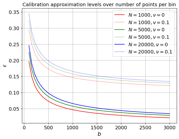
Figure 2: The relationship between $\epsilon$, number of points per bin $b$ and misspecification constant $\nu$ in Theorem 3.1. Based on the plot, when $\nu=0$, practitioners should set $b\simeq 300$ when $N=1000$, $b\simeq 400$ when $N=5000$, $b\simeq 500$ when $N=20000$ (attaining $\epsilon=0.1$). When a ground truth proxy is misspecified (Definition 3.2), e.g., $\nu=0.1$, for certain levels of $\epsilon$, the same bound can be attained with a larger $b$. For example, for achieving the same $\epsilon=0.15$, if $\nu=0$ then $b$ needs to be only approximately 250, whereas if $\nu=0.1$ then $b$ has to be $>1000$.

4 Related Work

Calibration for Language Models. Reinforcement learning from human feedback objective may prioritize adherence to user instructions in dialogue over producing well-calibrated predictions. (Kadavath et al., 2022). Lin et al. (2022) introduced the concept of verbalized confidence that prompts LMs to express confidence directly, focusing on fine-tuning, instead of zero-shot verbalized confidence. Mielke et al. (2022) uses an external calibrator for a white-box large language model. Other methods use consistency measures to improve LM calibration (Lyu et al., 2024). Our experimental setup closely relates to recent works in LM confidence elicitation (Tian et al., 2023; Xiong et al., 2024). These methods lack novel post-hoc calibrators and do not offer the rigorous calibration guarantees that ours provide. Calibration has been shown to impact selective QA performance Kamath et al. (2020), but they focus on uncertainty quantification and assumes that the LM allows access to the model likelihood.

Group Notions of Calibration. Previous works highlight the limitations of average-case calibration. Group-wise calibration, which uses predefined groupings (Kleinberg et al., 2017; Pleiss et al., 2017), has been adapted for language models (LMs). Li et al. (2024) train a model that approximates the precision-threshold curve for a given group by using few-shot samples to predict the LM’s empirical precision at various confidence thresholds. Ulmer et al. (2024) train an auxiliary model using accuracy per group as target to predict an LM’s confidence based on textual input and output. Detommaso et al. (2024) achieves multicalibration — simultaneous calibration across various intersecting groupings of the data. Our work complements multicalibration, and our methods could extend to this by adapting Algorithm 3 in Detommaso et al. (2024).  Luo et al. (2022) measure calibration over a set of similar predictions, quantified by a kernel function on feature space. Again, the notions of calibrations and their guarantees are incomparable.

Other Metrics for Measuring Calibration Error. Brier score (Brier, 1950) measures the accuracy of probabilistic predictions but while it can be decomposed into calibration and refinement (Blattenberger and Lad, 1985), it doesn’t directly assess calibration. As a result, a model with lower squared error may still be less well-calibrated. Maximum Calibration Error examines the maximum miscalibration across confidence bins (Guo et al., 2017), but in a QA setting, it faces the same issues as calibration error ($\text{CE}(h)$), as shown in Example 2.1. Through $\beta$-calibration, we present a principled and interpretable calibration target for QA settings.

5 Experiments

Datasets, Models, and Prompts. We use 5 QA datasets: TriviaQA (Joshi et al., 2017), SciQ (Welbl et al., 2017), BigBench (Srivastava et al., 2022), OpenBookQA (Mihaylov et al., 2018), and MMLU (Hendrycks et al., 2021) (see Table 4 for more details). We use two performant models: Mistral (Jiang et al., 2023) and Gemma (Team et al., 2024). To elicit confidence scores, we use two prompt techniques recently suggested in literature: Verb1S-Top1 & Ling1S-Top1 from Tian et al. (2023). See Table 5, (Appendix B.1) for details about the prompts.

Central to the implementation of posthoc calibration and evaluation of calibration is the availability of a label for a question-and-answer pair — specifically, whether the answer provided by the LM is accurate for the question posed by the user. In practice, a common idea to generate this label is to take an LM provided answer, and then use another LM to assess whether the proposed answer is semantically equivalent to the true (ground truth) answer (Tian et al., 2023). To construct the ground truth proxy for $y$, we use Llama 3.1 (Dubey et al., 2024).

Our Methods. We compare the performance of our calibrators: $\beta$-binning (BB) from Subsection 3.1 and hierarchical scaling-$\beta$-binning (HS-BB) from Subsection 3.2. We also include a fully pooled version of scaling-$\beta$-binning (S-BB), by setting $s[i]$ to a constant (thus, one partition) in Eq. ( 5). To set the hyperparameter minimum number of points per bin $b$ (Algorithm 1), we set an $\epsilon$ that is not too large as per Figure 2 and use root finding with the $\epsilon$ expression in Theorem 3.1 to choose $b$. We then search over a range of $b$’s by allowing for a misspecification range between $0$ and $0.05$ and a range of maximum kd-tree depths depending on the size of the dataset such that each partition admits a 3–10 bins. To set $B$ in UMD, we follow the guidelines in Gupta and Ramdas (2021). Note that their bound does not involve misspecification factor.

Baselines. We consider the following baselines: no recalibration (None) which returns state-of-the-art elicited confidence scores (Tian et al., 2023), histogram binning (UMD) (Gupta and Ramdas, 2021), Platt scaling (S) (Platt, 1999), and scaling-binning (S-B) (Kumar et al., 2019). These baselines consist of the state-of-the-art ideas in posthoc calibration. Note that the techniques UMD, S, and S-B, aim to minimize the expected calibration error CE (Definition 2.2) and do not take the partitions induced by $\beta$ into account.

Metrics. In this section, we primarily use two metrics for comparison. First, is the $\beta$-calibration error $\text{CE}(h;\beta)$ (Definition 2.4), which is the metric that our methods (presented in Section 3) optimize for. A lower $\text{CE}(h;\beta)$ indicates a more effective scheme for achieving $\beta$-calibration. As explained in Section 2, $\beta$-calibration error generalizes the expected calibration error ($\text{CE}(h)$).

Second, to measure the downstream impact of using $\beta$-calibration as the confidence calibration notion in a QA setting, we adapt selective question answering (Kamath et al., 2020) to our setting: given a threshold $\gamma\in[0,1]$, the answer $a$ is returned for a question $q$ to the end user if $h(q,a)\geq\tau$, and abstains (no answer is returned) otherwise. We adapt the area under risk-coverage curve, which is a standard way to evaluate selective prediction methods (El-Yaniv and Wiener, 2010) to our setting. Our post-hoc schemes produce discretized confidence scores $h$, often with large number of ties, which lead to unreliable risk-coverage calculations. Therefore, we consider the area under accuracy-confidence curve (AUAC): set grid points between 0 and 1, and for each grid point, record the accuracy (again, based on a ground truth proxy of $y$) of all points with a confidence score greater than or equal to that grid point. This accuracy is then used as the height of the curve. A higher AUAC indicates a more effective scheme for selective QA.

Training. We perform a 4-way (20:60:10:10) split of each dataset: the first is used to construct the kd-tree, second is used for posthoc calibration training, third is used for hyperparameter tuning and fourth is for testing. We find it crucial to optimize for AUAC during hyperparameter tuning as our schemes already aim to minimize $\text{CE}(h;\beta)$, obtaining the appropriate maximum kd-tree depth $d$ and binning parameters $b$ and $B$. Missing experimental details are presented in Appendix B.1.

Results. Table 2 shows the performance of the posthoc calibrators on MMLU and BigBench datasets. More results are provided in Tables 6 and 7. Our methods (BB, HS-BB, and S-BB) generally achieve the best $\beta$-calibration error $\text{CE}(h;\beta)$ and best area under the accuracy-confidence curve (AUAC). While the first result, in itself, may not be surprising as our proposed schemes aim to minimize $\text{CE}(h;\beta)$, the gap between our techniques and baselines is significantly huge. For example, notice the difference in the calibration error when just using the SOTA confidence elicitation prompts (None) from (Tian et al., 2023) vs. our schemes in Table 2. Among our schemes, HS-BB generally performs best. This is because a parametric model (especially a partially pooled model like hierarchical scaling) helps reduce the variance of the downstream binning averages.

For selective QA, we again notice that our proposed schemes consistently outperforms the baselines. In some cases, the underlying LLM using confidence elicitation prompts (None) is performant in selective answering and attains high AUAC (similar results using different LLMs were noted by Tian et al. (2023)), but are not well-calibrated as demonstrated by their high $\beta$-calibration score. Our schemes, S-BB and HS-BB are generally the top-two performing schemes for this task with comparable and in many cases better AUAC scores than the None scheme. Since the accuracy-confidence curve is generated by examining the accuracy of answers above a confidence threshold, the results demonstrate the desirable quality that the confidence scores provided by our proposed schemes are better at ranking accurate answers higher than inaccurate ones. Crucially, the lower performance of other baselines (like S-B, S, and B) demonstrates that the advantage of having a better calibration target that comes through our definition of $\beta$-calibration. In particular, our $\beta$-calibration framework identifies the optimal kd-tree depth, which is never equal to zero (the depth corresponding to standard average-case calibration) in our experiments.

6 Conclusions

We proposed $\beta$-calibration, a new notion of calibration which conditions on groups of QA pairs. We propose two new posthoc calibration schemes for LM-elicited confidence scores. Our algorithms are effective on various QA datasets. For future work, we plan to investigate alternative notions of calibration for groups, such as multi-calibration. Other choices of $\beta$ that generalize expected calibration error can also be used, such as random projection tree (Dasgupta and Freund, 2008), which adapts to the intrinsic low-dimensional structure in the data.

Limitations. The interpretability of the calibration guarantee for the user largely depends on the choice of $\beta$ — if users want the partitions to be very fine- or coarse-grained, then $\beta$ must be built with the appropriate depth. Furthermore, our algorithms assume that the output space of $\beta$ is fixed, which may be a limited assumption, given that the “information” space of generative QA may increase indefinitely over time.

Dataset Prompt LLM Calibrator $\text{CE}(h;\beta)$ AUAC MMLU Ling1s-Top1 Mistral BB (ours) $0.171\pm 0.005$ $0.20\pm 0.023$ MMLU Ling1s-Top1 Mistral HS-BB (ours) $\mathbf{0.16\pm 0.005}$ $\mathbf{0.269\pm 0.022}$ MMLU Ling1s-Top1 Mistral S-BB (ours) $0.163\pm 0.003$ $0.19\pm 0.045$ MMLU Ling1s-Top1 Mistral S-B $0.393\pm 0.004$ $0.141\pm 0.003$ MMLU Ling1s-Top1 Mistral S $0.249\pm 0.005$ $0.122\pm 0.002$ MMLU Ling1s-Top1 Mistral B $0.392\pm 0.003$ $0.139\pm 0.007$ MMLU Ling1s-Top1 Mistral None $0.532\pm 0.008$ $\mathbf{0.269\pm 0.007}$ MMLU Ling1s-Top1 Gemma BB (ours) $0.232\pm 0.005$ $0.211\pm 0.032$ MMLU Ling1s-Top1 Gemma HS-BB (ours) $0.182\pm 0.005$ $0.26\pm 0.01$ MMLU Ling1s-Top1 Gemma S-BB (ours) $\mathbf{0.181\pm 0.009}$ $\mathbf{0.275\pm 0.029}$ MMLU Ling1s-Top1 Gemma S-B $0.382\pm 0.006$ $0.184\pm 0.002$ MMLU Ling1s-Top1 Gemma S $0.201\pm 0.009$ $0.19\pm 0.003$ MMLU Ling1s-Top1 Gemma B $0.385\pm 0.003$ $0.183\pm 0.008$ MMLU Ling1s-Top1 Gemma None $0.603\pm 0.006$ $0.249\pm 0.01$ MMLU Verb1s-Top1 Mistral BB (ours) $0.197\pm 0.004$ $0.198\pm 0.046$ MMLU Verb1s-Top1 Mistral HS-BB (ours) $\mathbf{0.149\pm 0.004}$ $\mathbf{0.306\pm 0.035}$ MMLU Verb1s-Top1 Mistral S-BB (ours) $0.16\pm 0.004$ $0.217\pm 0.057$ MMLU Verb1s-Top1 Mistral S-B $0.362\pm 0.005$ $0.139\pm 0.004$ MMLU Verb1s-Top1 Mistral S $0.258\pm 0.005$ $0.126\pm 0.001$ MMLU Verb1s-Top1 Mistral B $0.352\pm 0.004$ $0.132\pm 0.011$ MMLU Verb1s-Top1 Mistral None $0.639\pm 0.006$ $0.255\pm 0.008$ MMLU Verb1s-Top1 Gemma BB (ours) $0.197\pm 0.006$ $\mathbf{0.345\pm 0.035}$ MMLU Verb1s-Top1 Gemma HS-BB (ours) $\mathbf{0.151\pm 0.006}$ $0.3\pm 0.035$ MMLU Verb1s-Top1 Gemma S-BB (ours) $0.161\pm 0.006$ $0.227\pm 0.074$ MMLU Verb1s-Top1 Gemma S-B $0.361\pm 0.007$ $0.133\pm 0.005$ MMLU Verb1s-Top1 Gemma S $0.228\pm 0.005$ $0.137\pm 0.004$ MMLU Verb1s-Top1 Gemma B $0.352\pm 0.004$ $0.144\pm 0.011$ MMLU Verb1s-Top1 Gemma None $0.636\pm 0.007$ $0.258\pm 0.006$ BigBench Ling1S-Top1 Mistral BB (ours) $0.195\pm 0.002$ $0.622\pm 0.009$ BigBench Ling1S-Top1 Mistral HS-BB (ours) $\mathbf{0.138\pm 0.006}$ $\mathbf{0.690\pm 0.031}$ BigBench Ling1S-Top1 Mistral S-BB (ours) $0.157\pm 0.010$ $0.641\pm 0.02$ BigBench Ling1S-Top1 Mistral S-B $0.387\pm 0.006$ $0.523\pm 0.006$ BigBench Ling1S-Top1 Mistral S $0.224\pm 0.003$ $0.52\pm 0.004$ BigBench Ling1S-Top1 Mistral B $0.379\pm 0.003$ $0.612\pm 0.017$ BigBench Ling1S-Top1 Mistral None $0.245\pm 0.004$ $0.684\pm 0.007$ BigBench Ling1S-Top1 Gemma BB (ours) $0.198\pm 0.006$ $0.41\pm 0.012$ BigBench Ling1S-Top1 Gemma HS-BB (ours) $\mathbf{0.142\pm 0.009}$ $\mathbf{0.421\pm 0.021}$ BigBench Ling1S-Top1 Gemma S-BB (ours) $0.193\pm 0.002$ $0.321\pm 0.052$ BigBench Ling1S-Top1 Gemma S-B $0.326\pm 0.002$ $0.302\pm 0.005$ BigBench Ling1S-Top1 Gemma S $0.180\pm 0.006$ $0.298\pm 0.005$ BigBench Ling1S-Top1 Gemma B $0.468\pm 0.001$ $0.293\pm 0.014$ BigBench Ling1S-Top1 Gemma None $0.427\pm 0.006$ $0.412\pm 0.01$

Table 2: Performance of our $\beta$-calibration methods, $\beta$-binning (BB), Pooled scaling-$\beta$-binning (S-BB) and Hierarchical scaling-$\beta$-binning (HS-BB)), compared to the baselines, UMD, (B,  (Gupta and Ramdas, 2021)), Platt Scaling (S, (Platt, 1999)), and Scaling-binning (S-B, (Kumar et al., 2019)), and prompt-based approach None (Tian et al., 2023) . The bold entry in the columns for $\text{CE}(h;\beta)$ and AUAC represent the best performing schemes for that metric. However, note that in some case the confidence intervals overlap, especially between our schemes.

Table 3: Important variables. Note that in our mathematical description, we treat the $k=3$ output answers and confidences as $3$ binary instances. Given a prompt function $m()$ and question $q$, at the end of an LM’s interaction, we obtain answers and confidences.

      Name       Notation       Description       Example       Question       $q$       Inputted question.       What happens to you if you eat watermelon seeds?       Ground truth       $a^{gt}$       Intended output answer. Note that we omit this in our mathematical description and work directly with the ground truth label $y$. In practice we use $a^{gt}$ to construct the ground truth proxy.       The watermelon seeds pass through your digestive system       Prompting function       $m()$       A function that converts the question into a specific form by inserting the question $q$. The example prompting function is Verb. 1S top-$k$ in Tian et al. [2023], with $k=3$. We denote the filled (by the question) prompt as $m(q)$. Note that multiple prompts may be generated (see the 2S prompts in  Tian et al. [2023])       Provide your three best guesses and the probability that each is correct (0.0 to 1.0) for the following question. Give ONLY the guesses and probabilities, no other words or explanation. For example: G1: <first most likely guess, as short as possible; not a complete sentence, just the guess! >P1: <the probability between 0.0 and 1.0 that G1 is correct, without any extra commentary whatsoever; just the probability!>… G3: <third most likely guess, as short as possible; not a complete sentence, just the guess!>P3: <the probability between 0.0 and 1.0 that G3 is correct, without any extra commentary whatsoever; just the probability!>. The question is: <$q$>       Answering function       $c(q)$       An answering function $c(q)=c(m(q))$, that models the pipeline, that takes as input $m(q)$ and outputs an answer $a$. This is invoked $k$ times to obtain $k$ answers. The function subsumes the postprocessing performed on the LM response to obtain answer $a$.       Implicitly-defined in the LM interaction       Answers       $(a^{1},a^{2},a^{3})$       Three sampled answers, obtained after text normalization of the LLM raw output.       (nothing, grow watermelon, stomachache)       Confidence function       $h(q,a)$       A confidence function $h(q,a)=h(m(q),a)$, that models the pipeline, that takes as input $m(q)$ and answer $a$ and outputs the confidence that the answer $a$ is correct for question $q$. This is invoked $k$ times to obtain $k$ confidences. The function subsumes the postprocessing performed on the LM response to obtain a float confidence value.       Implicitly-defined in the LM interaction       Confidence values       $(h^{1},h^{2},h^{3})$       Three confidence values associated with the three answers. Note that they may not be normalized.       (0.95, 0,05, 0.2)       Ground truth proxy (proxy of $y$)       $g(q,a,a^{gt})$       The returned truth value is postprocessed to map Yes/No to 1/0. In practice, this is used as a proxy ground truth. We also experimented with the query (checking for semantic equivalence) from Tian et al. [2023], but we observe a high false negative rate.       We query an LLM using the following prompt: Do following two answers to my question Q agree with each other? Q: <$q$>, A1: <$a^{1}$>, A2: <$a^{2}$>. Please answer with a single word, either “Yes." or “No.", and explain your reasoning.

Appendix A Additional Details for Section 3

A.1 Limitations of Non-discretized Methods

Estimation of $\mathbb{E}[Y|H]$ when $H=h(Q,A)$ is continuous is a difficult task [Kumar et al., 2019]. The confidence must also be discretized for it to achieve guarantees of marginal calibration [Gupta and Ramdas, 2021]. Prompts used to elicit confidence [Tian et al., 2023, Xiong et al., 2024] are not guaranteed to induce a discretized confidence score (both in the average-case- and $\beta$-calibration cases).

In practice, the estimation of $\text{CE}(h;\beta)$ is done by partitioning ${\mathcal{D}}$ according to $\beta$: ${\mathcal{D}}=\cup_{s=1}^{M}{\mathcal{D}}_{s}$, where ${\mathcal{D}}_{s}=\{(q_{i},a_{i},h_{i}y_{i}):\beta(q_{i},a_{i})=s\}$, and taking the weighted average of $\text{CE}(h)$’s (from Eq. ( 3)) from each ${\mathcal{D}}_{s}$ with weight $|{\mathcal{D}}_{s}|$. For each ${\mathcal{D}}_{s}$, $H$ is typically binned into intervals, and the calibration error in each bin is estimated as the difference between the average of confidence values and labels in that bin.

Lastly, estimation of $\text{CE}(h)$ for non-discretized methods may involve binning and can underestimate the error (Proposition 3.3 in [Kumar et al., 2019]). In our case, this is a possibility when comparing scaling against the other approaches.

A.2 Uniform-mass-double-dipping Histogram Binning (UMD)

We adapt UMD (Algorithm 1 from  Gupta and Ramdas [2021]) to our notation in Algorithm 4. UMD takes as input calibration data $\mathcal{D}=\{(h_{i},t_{i})\}_{i\in[N]}$, where $h_{i}$’s are (uncalibrated) confidence scores and $t_{i}$’s are the corresponding target labels. The function order-stats returns ordered confidence scores $(h_{(1)},\ldots,h_{(n)}$ where $h_{(1)}<h_{(2)}<\ldots<h_{(n)}$.

Algorithm 4 UMD

0:  Number of bins $B$, Calibration data $\mathcal{D}=\{(h_{i},t_{i})\}_{i\in[N]}$ (dataset cardinality $n$ depends on the inputted dataset, we refer to the dataset within the algorithm as ${\mathcal{D}}$.)

0:  Calibrator function $g_{\text{UMD}}:[0,1]\rightarrow[0,1]$

1:  $(h_{(1)},\ldots,h_{(n)})\leftarrow\text{order-stats}(h_{1},\ldots,h_{n})$

2:  $(t_{(1)},\ldots,t_{(n)}\leftarrow(t_{1},\ldots,t_{n})\text{ ordered as per the ordering of }(h_{(1)},\ldots,h_{(n)})$

3:  $\Delta\leftarrow\frac{(n+1)}{B}$

4:  $\hat{\Pi}\leftarrow\text{ empty array of size }B$

5:  $A\leftarrow 0\text{-indexed array}([0,\lceil\Delta\rceil,\lceil 2\Delta\rceil),\ldots,n+1]$

6:  for $b\leftarrow 1\text{ to }B$ do

7:     $l\leftarrow A_{b-1}$

8:     $u\leftarrow A_{b}$

9:     $\hat{\Pi}_{b}\leftarrow\text{mean}(t_{(l+1)}\ldots,t_{(u-1)})$

10:  end for

11:  $(h_{(0)},h_{(n+1)})\leftarrow(0,1)$

12:  Define the calibrator function, $g_{\text{UMD}}$: $g_{\text{UMD}}(h_{\text{test}})=\sum_{b=1}^{B}\mathbf{1}\{h_{(A_{b-1})}\leq h_{\text{test}}<h_{(A_{b})}\}\hat{\Pi}_{b}$

13:  return  $g_{\text{UMD}}$

A.3 Distribution-free Guarantees

In Gupta et al. [2020], UMD procedure (Algorithm 4) is assumed to take ground truth $y$ as input ($t=y$). Since in our setting, it is possible to pass a proxy ground truth, we now describe a generalization of conditional calibration guarantees of UMD procedure [Gupta and Ramdas, 2021, Theorem 3].

Theorem A.1 (Conditional Calibration Guarantee of Algorithm 4 under Label Misspecification).

Consider an input calibration dataset $\tilde{D}$ defined in Section 3.3 with misspecification factor $\nu$ from Definition 3.2. Assume that the $h_{i}$’s are distinct and $N\geq 2B$. Then calibrator $g_{\text{UMD}}$ outputted by Algorithm 4, with input ${\mathcal{D}}=\tilde{D}$, is $(\epsilon,\alpha)$-conditionally calibrated for any $\alpha\in(0,1)$, with

$$\epsilon=\sqrt{\frac{\log(2B/\alpha)}{2(\lfloor N/B\rfloor-1)}}+\nu.$$ (6)

Proof.

For $b\in\{0,1,\ldots,B\}$, define $k_{b}=\lceil b(N+1/B)\rceil$. Fix $h_{(0)}:=0$ and $h_{(N+1)}:=1$ as the smallest and largest order statistics, respectively. As per Algorithm 4, we compute the order statistics of the input data and gather the following points into a set: ${\mathcal{M}}:=\{h_{(k_{1})},\ldots,h_{k_{(B-1)}}\}$.

Let ${\mathcal{B}}:[0,1]\rightarrow[B]$ be the binning function: ${\mathcal{B}}(H)=b\iff h_{(k_{b-1})}\leq g_{\text{UMD}}(H)<h_{(k_{b})}$. Given ${\mathcal{M}}$, the function ${\mathcal{B}}$ is deterministic, i.e., for every $b\in[B]$, $\mathbb{E}[\tilde{Y}|{\mathcal{B}}(H)=b]$ is deterministic.

Consider some $b\in\{0,1,\ldots,B\}$ and denote $l=k_{b-1},u=k_{b}$. By Lemma 2 from [Gupta and Ramdas, 2021], the unordered (denoted by $h_{\{\cdot\}}$) confidence scores $h_{\{l+1\}},h_{\{l+2\}},\ldots,h_{\{u+1\}}$ are i.i.d given ${\mathcal{M}}$, with the same conditional distribution as that of $H$ given ${\mathcal{B}}(H)=b$. Therefore, $\tilde{y}_{\{l+1\}},\tilde{y}_{\{l+2\}},\ldots,\tilde{y}_{\{u-1\}}$ are i.i.d given ${\mathcal{S}}$, with the conditional distribution $\text{Bernoulli}(\mathbb{E}[\tilde{Y}\mid{\mathcal{B}}(H)=b]$.

We now show that $\hat{\Pi}_{b}$ (defined in Line 9 and returned by $g_{\text{UMD}}$ in Line 12 in Algorithm 4), the average of the $\tilde{y}$ in a bin $b$ values, concentrates around $\mathbb{E}[\tilde{Y}\mid{\mathcal{B}}(H)=b]$. For any $\gamma\in(0,1)$, by Hoeffding’s inequality, w.p. at least $1-\gamma$:

$$\left|\mathbb{E}[\tilde{Y}|{\mathcal{B}}(H)=b]-\hat{\Pi}_{b}\right|\leq\sqrt{\frac{\log(2/\gamma)}{2\lfloor u-l-1\rfloor}}\leq\sqrt{\frac{\log(2/\gamma)}{2(\lfloor N/B\rfloor-1)}},$$ (7)

where the second inequality holds since for any $b$, $u-l=\lfloor(b+1)(N+1)/B\rfloor-\lfloor b(N+1)/B\rfloor\geq\lfloor N/B\rfloor$. Using law of total probability (partitioning $\{{\mathcal{B}}(h)=b\}$ to $\{h:{\mathcal{B}}(h)=b\}$), we obtain:

$$\mathbb{E}[\tilde{Y}\mid{\mathcal{B}}(H)=b]\leq\left|\mathbb{E}[Y\mid{\mathcal{B}}(H)=b]-\nu\right|,$$

which implies that

$$\left|\mathbb{E}[Y\mid{\mathcal{B}}(H)=b]-\hat{\Pi}_{b}\right|\leq\sqrt{\frac{\log(2/\gamma)}{2(\lfloor N/B\rfloor-1)}}+\nu.$$ (8)

Set $\gamma=\alpha/B$ in Eq. ( 8), and take a union bound over all $b\in B$. With probability at least $1-\alpha$, for every $b\in B$, $\left|\mathbb{E}[Y|{\mathcal{B}}(H)=b]-\hat{\Pi}_{b}\right|\leq\epsilon$, where $\epsilon$ is the RHS of Eq. ( 8). This implies that:

$$\left|\mathbb{E}[Y\mid H]-H\right| =\left|\mathbb{E}[\mathbb{E}[Y\mid{\mathcal{B}}(H),H]\mid H]-H\right|$$

$$=\left|\mathbb{E}[\mathbb{E}[Y\mid{\mathcal{B}}(H)]\mid H]-H\right|$$

$$=\left|\mathbb{E}[\mathbb{E}[Y\mid{\mathcal{B}}(H)]-H\mid H\right|$$

$$=\left|\mathbb{E}[\mathbb{E}[Y\mid{\mathcal{B}}(H)]-\hat{\Pi}_{{\mathcal{B}}(H)}\mid H\right|$$

$$\leq\mathbb{E}\left[\left|\mathbb{E}[Y\mid{\mathcal{B}}(H)]-\hat{\Pi}_{{\mathcal{B}}(H)}\right|\mid H\right]$$

$$\leq\epsilon,$$

Where the first equality is due to the law of total expectation, the fourth equality is by the definition of the quantity returned by $g_{\text{UMD}}$, and the first inequality is due to Jensen’s inequality. This completes the proof, showing that $g_{\text{UMD}}$ is $(\epsilon,\alpha)$-conditionally calibrated for any $\alpha\in(0,1)$. ∎

See 3.1

Proof.

For $s\in{\mathcal{S}}$, let $P_{s}$ denote the distribution of $(h,\tilde{y})$ conditional on $\beta(q,a)=s$. The tuples in ${\mathcal{D}}_{s}$ are i.i.d. samples from $P_{s}$ and $g_{s}={\mathcal{G}}[s]$ is the corresponding fitted UMD calibrator. The number of bins is $B_{s}=\lfloor n_{s}/b\rfloor$. Since, $n_{s}\geq b\lfloor n_{s}/b\rfloor\geq 2B_{s}$,

Let $B=\sum_{s=1}^{S}B_{s}$ and $\alpha_{s}=\alpha B_{s}/B$. Note that $B\leq\sum_{s\in{\mathcal{S}}}n_{s}/b=N/b$. We apply the bound in Theorem A.1 to obtain:

$${\mathbb{P}}\left(\forall p\in\text{range}(g_{s}),\left|\mathbb{E}\left[\tilde{Y}|\beta(q,a)=s,g_{s}(h)=p\right]-p\right|\leq\sqrt{\frac{\log(2B_{s}/\alpha)}{2(\lfloor n_{s}/B_{s}\rfloor-1)}}+\nu\leavevmode\nobreak\ \Bigg{|}\leavevmode\nobreak\ \beta(q,a)=s\right)$$

$$\geq 1-\alpha_{s}.$$

Note that

$$\sqrt{\frac{\log(2B_{s}/\alpha_{s})}{2(\lfloor n_{s}/B_{s}\rfloor-1)}}= \sqrt{\frac{\log(2B/\alpha)}{2(\lfloor n_{s}/B_{s}\rfloor-1)}}\leq\sqrt{\frac{\log(2N/b\alpha)}{2(\lfloor n_{s}/B_{s}\rfloor-1)}}\leq\sqrt{\frac{\log(2N/b\alpha)}{2(b-1)}}.$$

For every $s\in{\mathcal{S}}$:

$${\mathbb{P}}\left(\forall p\in\text{range}(g_{s}),\left|\mathbb{E}\left[\tilde{Y}|\beta(q,a)=s,g_{s}(h)=p\right]-p\right|\leq\epsilon\leavevmode\nobreak\ \Bigg{|}\leavevmode\nobreak\ \beta(q,a)=s\right)\geq 1-\alpha_{s}.$$

Taking union bound over $S$ gives:

$${\mathbb{P}}\left(\forall s\in{\mathcal{S}},\forall p\in\text{range}(g_{s}),\left|\mathbb{E}\left[\tilde{Y}|\beta(q,a)=s,g_{s}(h)=p\right]-p\right|\leq\epsilon\leavevmode\nobreak\ \Bigg{|}\leavevmode\nobreak\ \beta(q,a)=s\right) \geq 1-\sum_{s\in{\mathcal{S}}}\alpha_{s}$$

$$=1-\alpha.$$

This completes the proof. ∎

To remove the assumption that $h_{i}$’s are distinct in Theorem 3.1, we could use the randomized version of UMD (Algorithm 2 in  Gupta and Ramdas [2021]). This adds an additive factor to $\epsilon$ in Theorem 3.1 but can be made arbitrarily small. For simplicity, we have chosen to provide the guarantees for the non-randomized version of UMD.

Appendix B Additional Details for Section 5

B.1 Missing Experimental Details

Details on LM Querying. We set the LM temperature to close to 0 to minimize output stochasticity and set max tokens to be able to process the prompt $m(q)$. We include the prompts in Table 5. The variable EXPRESSION$\_$LIST in Ling1S-Top1 prompt is taken from Fagen-Ulmschneider [2015].

Compute Resources. The experiments were run using a 3090Ti GPU and 64 GB of RAM.

Training Details. We perform random splitting 8 times using different seeds and use the repeated measures to form our confidence intervals. We set the number of bins $B$ in the UMD baseline and scaling-binning by deriving hyperparameter search ranges from setting different $\epsilon$s in Theorem 3 in [Gupta and Ramdas, 2021]. We describe how we set the number of points per bin $b$ in Algorithm 1 and Algorithm 3 in Section 5. We have also attempted to ensure that for every $B$ we can find in its hyperparameter tuning range, there is a $b$ in its hyperparameter tuning range, such that $B=\lfloor N/b\rfloor$. This correspondence, coupled with the same target variable to optimize, helps isolate the impact of $\beta$ on post-hoc calibration.

Table 4: Dataset statistics. Multiple-choice QA datasets provide a set of possible answers. We add additional prompt text for them, see Table 5.

     Dataset      Size      Type      SciQ      11609      QA      Bigbench      20320      QA      MMLU      13869      Multiple-choice QA      OpenBookQA      4835      Multiple-choice QA      TriviaQA      11313      QA

Table 5: Prompts used in the experiments.

      Prompt Name       Prompt Template       Verb1S-Top1       Provide your best guess and the probability that it is correct (0.0 to 1.0) for the following question. Give ONLY the guess and probability, no other words or explanation. For example: Guess: <most likely guess, as short as possible; not a complete sentence, just the guess! >  Probability: <the probability between 0.0 and 1.0 that your guess is correct, without any extra commentary whatsoever; just the probability! >  The question is: <$q$>.       Ling1S-Top1       Provide your best guess for the following question, and describe how likely it is that your guess is correct as one of the following expressions: $EXPRESSION_LIST. Give ONLY the guess and your confidence, no other words or explanation. For example: Guess: <most likely guess, as short as possible; not a complete sentence, just the guess!>  Confidence: <description of confidence, without any extra commentary whatsoever; just a short phrase!>   The question is: <q >       Additional prompt text for multiple-choice QA task with a set of choices $C$       The answer must be chosen from the following list of size <$|C|$>: <$C$ >. Only the actual answer (not the choice number or index) from the list should be used in the response.       ground truth proxy       See the example for ground truth Proxy in Table 3.

Table 6: (Continuation of Table 2) Performance of our $\beta$-calibration methods.

.      Dataset      Prompt      LLM      Calibrator      $\text{CE}(h;\beta)$      AUAC      SciQ      Ling1S-Top1      Mistral      BB (ours)      $\mathbf{0.165\pm 0.003}$      $\mathbf{0.482\pm 0.024}$      SciQ      Ling1S-Top1      Mistral      HS-BB (ours)      $0.175\pm 0.004$      $0.437\pm 0.028$      SciQ      Ling1S-Top1      Mistral      S-BB (ours)      $0.171\pm 0.006$      $0.426\pm 0.034$      SciQ      Ling1S-Top1      Mistral      S-B      $0.466\pm 0.003$      $0.21\pm 0.007$      SciQ      Ling1S-Top1      Mistral      S      $0.255\pm 0.005$      $0.21\pm 0.005$      SciQ      Ling1S-Top1      Mistral      B      $0.457\pm 0.003$      $0.356\pm 0.025$      SciQ      Ling1S-Top1      Mistral      None      $0.366\pm 0.011$      $0.451\pm 0.009$      SciQ      Ling1S-Top1      Gemma      BB (ours)      $0.158\pm 0.011$      $0.357\pm 0.023$      SciQ      Ling1S-Top1      Gemma      HS-BB (ours)      $0.148\pm 0.011$      $0.363\pm 0.032$      SciQ      Ling1S-Top1      Gemma      S-BB (ours)      $\mathbf{0.146\pm 0.006}$      $0.366\pm 0.085$      SciQ      Ling1S-Top1      Gemma      S-B      $0.485\pm 0.003$      $0.194\pm 0.014$      SciQ      Ling1S-Top1      Gemma      S      $0.211\pm 0.008$      $0.191\pm 0.008$      SciQ      Ling1S-Top1      Gemma      B      $0.486\pm 0.003$      $0.195\pm 0.011$      SciQ      Ling1S-Top1      Gemma      None      $0.446\pm 0.011$      $\mathbf{0.403\pm 0.018}$      SciQ      Verb1S-Top1      Mistral      BB (ours)      $0.262\pm 0.009$      $0.428\pm 0.027$      SciQ      Verb1S-Top1      Mistral      HS-BB (ours)      $0.203\pm 0.006$      $\mathbf{0.474\pm 0.048}$      SciQ      Verb1S-Top1      Mistral      S-BB (ours)      $\mathbf{0.182\pm 0.006}$      $\mathbf{0.474\pm 0.095}$      SciQ      Verb1S-Top1      Mistral      S-B      $0.472\pm 0.003$      $0.237\pm 0.006$      SciQ      Verb1S-Top1      Mistral      S      $0.228\pm 0.005$      $0.27\pm 0.02$      SciQ      Verb1S-Top1      Mistral      B      $0.458\pm 0.002$      $0.377\pm 0.012$      SciQ      Verb1S-Top1      Mistral      None      $0.451\pm 0.013$      $0.451\pm 0.015$      SciQ      Verb1S-Top1      Gemma      BB (ours)      $0.268\pm 0.005$      $0.278\pm 0.021$      SciQ      Verb1S-Top1      Gemma      HS-BB (ours)      $0.194\pm 0.006$      $0.386\pm 0.034$      SciQ      Verb1S-Top1      Gemma      S-BB (ours)      $\mathbf{0.182\pm 0.005}$      $0.279\pm 0.023$      SciQ      Verb1S-Top1      Gemma      S-B      $0.477\pm 0.002$      $0.149\pm 0.013$      SciQ      Verb1S-Top1      Gemma      S      $0.243\pm 0.007$      $0.246\pm 0.008$      SciQ      Verb1S-Top1      Gemma      B      $0.464\pm 0.003$      $0.344\pm 0.021$      SciQ      Verb1S-Top1      Gemma      None      $0.495\pm 0.01$      $\mathbf{0.421\pm 0.01}$      TriviaQA      Ling1S-Top1      Mistral      BB (ours)      $0.26\pm 0.003$      $0.467\pm 0.024$      TriviaQA      Ling1S-Top1      Mistral      HS-BB (ours)      $0.195\pm 0.007$      $0.499\pm 0.014$      TriviaQA      Ling1S-Top1      Mistral      S-BB (ours)      $\mathbf{0.184\pm 0.005}$      $\mathbf{0.541\pm 0.021}$      TriviaQA      Ling1S-Top1      Mistral      S-B      $0.441\pm 0.003$      $0.275\pm 0.006$      TriviaQA      Ling1S-Top1      Mistral      S      $0.266\pm 0.005$      $0.28\pm 0.006$      TriviaQA      Ling1S-Top1      Mistral      B      $0.432\pm 0.003$      $0.441\pm 0.009$      TriviaQA      Ling1S-Top1      Mistral      None      $0.326\pm 0.008$      $0.537\pm 0.01$      TriviaQA      Ling1S-Top1      Gemma      BB (ours)      $0.268\pm 0.007$      $0.310\pm 0.034$      TriviaQA      Ling1S-Top1      Gemma      HS-BB (ours)      $0.188\pm 0.02$      $\mathbf{0.359\pm 0.035}$      TriviaQA      Ling1S-Top1      Gemma      S-BB (ours)      $\mathbf{0.18\pm 0.005}$      $0.351\pm 0.051$      TriviaQA      Ling1S-Top1      Gemma      S-B      $0.235\pm 0.015$      $0.310\pm 0.007$      TriviaQA      Ling1S-Top1      Gemma      S      $0.211\pm 0.012$      $0.086\pm 0.005$      TriviaQA      Ling1S-Top1      Gemma      B      $0.468\pm 0.003$      $0.199\pm 0.019$      TriviaQA      Ling1S-Top1      Gemma      None      $0.486\pm 0.01$      $0.349\pm 0.007$      TriviaQA      Verb1S-Top1      Mistral      BB (ours)      $0.242\pm 0.006$      $\mathbf{0.618\pm 0.016}$      TriviaQA      Verb1S-Top1      Mistral      HS-BB (ours)      $0.191\pm 0.01$      $0.573\pm 0.024$      TriviaQA      Verb1S-Top1      Mistral      S-BB (ours)      $\mathbf{0.18\pm 0.006}$      $0.545\pm 0.029$      TriviaQA      Verb1S-Top1      Mistral      S-B      $0.436\pm 0.005$      $0.324\pm 0.007$      TriviaQA      Verb1S-Top1      Mistral      S      $0.27\pm 0.005$      $0.352\pm 0.014$      TriviaQA      Verb1S-Top1      Mistral      B      $0.409\pm 0.005$      $0.525\pm 0.019$      TriviaQA      Verb1S-Top1      Mistral      None      $0.38\pm 0.01$      $0.582\pm 0.011$      TriviaQA      Verb1S-Top1      Gemma      BB (ours)      $0.249\pm 0.006$      $0.381\pm 0.02$      TriviaQA      Verb1S-Top1      Gemma      HS-BB (ours)      $0.192\pm 0.006$      $\mathbf{0.417\pm 0.034}$      TriviaQA      Verb1S-Top1      Gemma      S-BB (ours)      $\mathbf{0.183\pm 0.008}$      $0.337\pm 0.038$      TriviaQA      Verb1S-Top1      Gemma      S-B      $0.444\pm 0.003$      $0.231\pm 0.012$      TriviaQA      Verb1S-Top1      Gemma      S      $0.258\pm 0.008$      $0.225\pm 0.006$      TriviaQA      Verb1S-Top1      Gemma      B      $0.429\pm 0.004$      $0.37\pm 0.015$      TriviaQA      Verb1S-Top1      Gemma      None      $0.527\pm 0.008$      $\mathbf{0.417\pm 0.008}$

Table 7: (Continuation of Table 2) Performance of our $\beta$-calibration methods.

.      Dataset      Prompt      LLM      Calibrator      $\text{CE}(h;\beta)$      AUAC      OpenBookQA      Ling1S-Top1      Mistral      BB (ours)      $0.285\pm 0.009$      $0.353\pm 0.043$      OpenBookQA      Ling1S-Top1      Mistral      HS-BB (ours)      $0.211\pm 0.015$      $0.37\pm 0.065$      OpenBookQA      Ling1S-Top1      Mistral      S-BB (ours)      $\mathbf{0.193\pm 0.012}$      $0.34\pm 0.062$      OpenBookQA      Ling1S-Top1      Mistral      S-B      $0.477\pm 0.002$      $0.135\pm 0.004$      OpenBookQA      Ling1S-Top1      Mistral      S      $0.32\pm 0.006$      $0.133\pm 0.005$      OpenBookQA      Ling1S-Top1      Mistral      B      $0.471\pm 0.004$      $0.255\pm 0.023$      OpenBookQA      Ling1S-Top1      Mistral      None      $0.441\pm 0.013$      $\mathbf{0.38\pm 0.015}$      OpenBookQA      Ling1S-Top1      Gemma      BB (ours)      $0.316\pm 0.01$      $0.25\pm 0.028$      OpenBookQA      Ling1S-Top1      Gemma      HS-BB (ours)      $0.221\pm 0.016$      $0.261\pm 0.032$      OpenBookQA      Ling1S-Top1      Gemma      S-BB (ours)      $\mathbf{0.215\pm 0.011}$      $0.257\pm 0.082$      OpenBookQA      Ling1S-Top1      Gemma      S-B      $0.415\pm 0.005$      $0.129\pm 0.009$      OpenBookQA      Ling1S-Top1      Gemma      S      $0.421\pm 0.01$      $0.152\pm 0.013$      OpenBookQA      Ling1S-Top1      Gemma      B      $0.483\pm 0.003$      $0.12\pm 0.017$      OpenBookQA      Ling1S-Top1      Gemma      None      $0.434\pm 0.015$      $\mathbf{0.31\pm 0.017}$      OpenBookQA      Verb1S-Top1      Mistral      BB (ours)      $0.288\pm 0.008$      $0.338\pm 0.035$      OpenBookQA      Verb1S-Top1      Mistral      HS-BB (ours)      $0.232\pm 0.012$      $\mathbf{0.344\pm 0.018}$      OpenBookQA      Verb1S-Top1      Mistral      S-BB (ours)      $\mathbf{0.225\pm 0.011}$      $0.316\pm 0.027$      OpenBookQA      Verb1S-Top1      Mistral      S-B      $0.445\pm 0.006$      $0.331\pm 0.011$      OpenBookQA      Verb1S-Top1      Mistral      S      $0.282\pm 0.01$      $0.3\pm 0.009$      OpenBookQA      Verb1S-Top1      Mistral      B      $0.447\pm 0.003$      $0.28\pm 0.02$      OpenBookQA      Verb1S-Top1      Mistral      None      $0.561\pm 0.018$      $0.311\pm 0.021$      OpenBookQA      Verb1S-Top1      Gemma      S-BB (ours)      $\mathbf{0.228\pm 0.011}$      $\mathbf{0.343\pm 0.027}$      OpenBookQA      Verb1S-Top1      Gemma      S-B      $0.410\pm 0.006$      $0.301\pm 0.011$      OpenBookQA      Verb1S-Top1      Gemma      S      $0.298\pm 0.01$      $0.280\pm 0.011$      OpenBookQA      Verb1S-Top1      Gemma      B      $0.447\pm 0.003$      $0.293\pm 0.04$      OpenBookQA      Verb1S-Top1      Gemma      None      $0.561\pm 0.018$      $0.315\pm 0.036$      OpenBookQA      Verb1S-Top1      Gemma      BB (ours)      $0.261\pm 0.008$      $0.332\pm 0.048$      OpenBookQA      Verb1S-Top1      Gemma      HS-BB (ours)      $\mathbf{0.228\pm 0.012}$      $0.321\pm 0.011$      BigBench      Verb1S-Top1      Mistral      BB (ours)      $0.161\pm 0.003$      $0.665\pm 0.031$      BigBench      Verb1S-Top1      Mistral      HS-BB (ours)      $\mathbf{0.132\pm 0.009}$      $0.672\pm 0.079$      BigBench      Verb1S-Top1      Mistral      S-BB (ours)      $0.134\pm 0.004$      $\mathbf{0.679\pm 0.012}$      BigBench      Verb1S-Top1      Mistral      S-B      $0.361\pm 0.006$      $0.513\pm 0.016$      BigBench      Verb1S-Top1      Mistral      S      $0.208\pm 0.004$      $0.522\pm 0.018$      BigBench      Verb1S-Top1      Mistral      B      $0.351\pm 0.002$      $0.592\pm 0.014$      BigBench      Verb1S-Top1      Mistral      None      $0.248\pm 0.005$      $0.671\pm 0.005$      BigBench      Verb1S-Top1      Gemma      BB (ours)      $0.171\pm 0.003$      $\mathbf{0.503\pm 0.019}$      BigBench      Verb1S-Top1      Gemma      HS-BB (ours)      $\mathbf{0.159\pm 0.006}$      $0.502\pm 0.011$      BigBench      Verb1S-Top1      Gemma      S-BB (ours)      $0.215\pm 0.005$      $0.465\pm 0.024$      BigBench      Verb1S-Top1      Gemma      S-B      $0.456\pm 0.001$      $0.289\pm 0.011$      BigBench      Verb1S-Top1      Gemma      S      $0.259\pm 0.004$      $0.292\pm 0.007$      BigBench      Verb1S-Top1      Gemma      B      $0.431\pm 0.002$      $0.441\pm 0.014$      BigBench      Verb1S-Top1      Gemma      None      $0.458\pm 0.01$      $0.499\pm 0.01$

Appendix C KD-tree construction for $\beta$-calibration

We adapt kd-tree [Bentley, 1975] to construct our $\beta$ partitions. We first recall the standard construction of a kd-tree. Let $Z_{i}=(Z_{i1},\ldots,Z_{im},\ldots,Z_{iM}),i=1,\ldots,N$ be the $M$-dimensional dataset to bin and let $H^{k}$ with $k=0$ represent $\{Z_{1},\ldots,Z_{N}\}$. Let $z^{k}_{m}$ denote the median of all the $m$th coordinates of the $Z$s in $H^{k}$. Let $Z[p]$ denote the $p$th coordinate of a $Z$ vector. Set base case value of $k=0$.

The partitioning scheme to be applied recursively is as follows: split $H^{k}$ into two halfspaces by pivoting on $z^{k}_{m}$, to obtain $H^{2k+1}:=\left\{Z\in H^{k}:Z[p]\leq z^{k}_{m}\right\}$ and $H^{2k+2}:=\left\{Z\in H^{k}:Z[p]>z^{k}_{m}\right\}$. The coordinate index $m$ is set to $\lfloor\log 2\rfloor(k+1)+1$, i.e., as we split the nodes, we only change the coordinate index when we switch to another level. When we reach $m=M$, we reset $m=0$.

In our setting, we form bounded spaces so that our calibrators that contain a $\beta$-binning subroutine can generalize well during test time (outliers that are the closest to the boundary of a space will not be assigned to that space). We take the observations with the smallest and largest order statistic in each coordinate used for pivoting, and use them as bounding values for that coordinate.

At test-time, an $M$-vector instance is inserted into one of the leaves by following the same rule as in the partitioning scheme. If any coordinate value is outside its bounding values, assign it to none of the leaves. Otherwise, cycle through the $M$ coordinates and assign the instance to the left tree if the coordinate is less than or equal to $z^{k}_{m}$, or to the right tree otherwise. Repeat until a leaf is reached.

References

- Achiam et al. [2023] Josh Achiam, Steven Adler, Sandhini Agarwal, Lama Ahmad, Ilge Akkaya, Florencia Leoni Aleman, Diogo Almeida, Janko Altenschmidt, Sam Altman, and Shyamal Anadkat. GPT-4 technical report. arXiv:2303.08774, 2023.
- Bentley [1975] Jon Louis Bentley. Multidimensional binary search trees used for associative searching. Communications of the ACM, 18(9):509–517, 1975.
- Blattenberger and Lad [1985] Gail Blattenberger and Frank Lad. Separating the brier score into calibration and refinement components: A graphical exposition. The American Statistician, 39(1):26–32, 1985.
- Brier [1950] Glenn W Brier. Verification of forecasts expressed in terms of probability. Monthly weather review, 78(1):1–3, 1950.
- Brown et al. [2020] Tom Brown, Benjamin Mann, Nick Ryder, Melanie Subbiah, Jared D Kaplan, Prafulla Dhariwal, Arvind Neelakantan, Pranav Shyam, Girish Sastry, and Amanda Askell. Language models are few-shot learners. Advances in Neural Information Processing Systems, 33:1877–1901, 2020.
- Chowdhery et al. [2023] Aakanksha Chowdhery, Sharan Narang, Jacob Devlin, Maarten Bosma, Gaurav Mishra, Adam Roberts, Paul Barham, Hyung Won Chung, Charles Sutton, and Sebastian Gehrmann. Palm: Scaling language modeling with pathways. Journal of Machine Learning Research, 24(240):1–113, 2023.
- Dasgupta and Freund [2008] Sanjoy Dasgupta and Yoav Freund. Random projection trees and low dimensional manifolds. In Proceedings of the fortieth annual ACM symposium on Theory of computing, pages 537–546, 2008.
- Detommaso et al. [2024] Gianluca Detommaso, Martin Bertran, Riccardo Fogliato, and Aaron Roth. Multicalibration for confidence scoring in LLMs. In International Conference on Machine Learning, 2024.
- Dubey et al. [2024] Abhimanyu Dubey, Abhinav Jauhri, Abhinav Pandey, Abhishek Kadian, Ahmad Al-Dahle, Aiesha Letman, Akhil Mathur, Alan Schelten, Amy Yang, Angela Fan, et al. The Llama 3 herd of models. arXiv preprint arXiv:2407.21783, 2024.
- El-Yaniv and Wiener [2010] Ran El-Yaniv and Yair Wiener. On the foundations of noise-free selective classification. Journal of Machine Learning Research, 11(5), 2010.
- Fagen-Ulmschneider [2015] Wade Fagen-Ulmschneider. Perception of probability words. 2015. URL https://waf.cs.illinois.edu/visualizations/Perception-of-Probability-Words/. Accessed: 2024-05-21.
- Goldstein [2011] Harvey Goldstein. Multilevel statistical models. John Wiley & Sons, 2011.
- Guo et al. [2017] Chuan Guo, Geoff Pleiss, Yu Sun, and Kilian Q Weinberger. On calibration of modern neural networks. In International Conference on Machine Learning, pages 1321–1330. PMLR, 2017.
- Gupta and Ramdas [2021] Chirag Gupta and Aaditya Ramdas. Distribution-free calibration guarantees for histogram binning without sample splitting. In International Conference on Machine Learning, pages 3942–3952. PMLR, 2021.
- Gupta et al. [2020] Chirag Gupta, Aleksandr Podkopaev, and Aaditya Ramdas. Distribution-free binary classification: prediction sets, confidence intervals and calibration. Advances in Neural Information Processing Systems, 33:3711–3723, 2020.
- Hendrycks et al. [2021] Dan Hendrycks, Collin Burns, Steven Basart, Andy Zou, Mantas Mazeika, Dawn Song, and Jacob Steinhardt. Measuring massive multitask language understanding. In International Conference on Learning Representations, 2021.
- Huang et al. [2023] Lei Huang, Weijiang Yu, Weitao Ma, Weihong Zhong, Zhangyin Feng, Haotian Wang, Qianglong Chen, Weihua Peng, Xiaocheng Feng, and Bing Qin. A survey on hallucination in large language models: Principles, taxonomy, challenges, and open questions. arXiv:2311.05232, 2023.
- Jiang et al. [2023] Albert Q Jiang, Alexandre Sablayrolles, Arthur Mensch, Chris Bamford, Devendra Singh Chaplot, Diego de las Casas, Florian Bressand, Gianna Lengyel, Guillaume Lample, Lucile Saulnier, et al. Mistral 7b. arXiv preprint arXiv:2310.06825, 2023.
- Joshi et al. [2017] Mandar Joshi, Eunsol Choi, Daniel S Weld, and Luke Zettlemoyer. TriviaQA: A large scale distantly supervised challenge dataset for reading comprehension. In Proceedings of the 55th Annual Meeting of the Association for Computational Linguistics, 2017.
- Kadavath et al. [2022] Saurav Kadavath, Tom Conerly, Amanda Askell, Tom Henighan, Dawn Drain, Ethan Perez, Nicholas Schiefer, Zac Hatfield-Dodds, Nova DasSarma, and Eli Tran-Johnson. Language models (mostly) know what they know. arXiv:2207.05221, 2022.
- Kamath et al. [2020] Amita Kamath, Robin Jia, and Percy Liang. Selective question answering under domain shift. In Proceedings of the 58th Annual Meeting of the Association for Computational Linguistics, 2020.
- Kleinberg et al. [2017] Jon Kleinberg, Sendhil Mullainathan, and Manish Raghavan. Inherent trade-offs in the fair determination of risk scores. Innovations in Theoretical Computer Science Conference (ITCS), 2017.
- Kuhn et al. [2023] Lorenz Kuhn, Yarin Gal, and Sebastian Farquhar. Semantic uncertainty: Linguistic invariances for uncertainty estimation in natural language generation. International Conference on Learning Representations, 2023.
- Kumar et al. [2019] Ananya Kumar, Percy S Liang, and Tengyu Ma. Verified uncertainty calibration. Advances in Neural Information Processing Systems, 32, 2019.
- Li et al. [2024] Xiang Lisa Li, Urvashi Khandelwal, and Kelvin Guu. Few-shot recalibration of language models. arXiv:2403.18286, 2024.
- Lin et al. [2022] Stephanie Lin, Jacob Hilton, and Owain Evans. Teaching models to express their uncertainty in words. Transactions of Machine Learning Research, 2022.
- Luo et al. [2022] Rachel Luo, Aadyot Bhatnagar, Yu Bai, Shengjia Zhao, Huan Wang, Caiming Xiong, Silvio Savarese, Stefano Ermon, Edward Schmerling, and Marco Pavone. Local calibration: Metrics and recalibration. In Uncertainty in Artificial Intelligence, pages 1286–1295. PMLR, 2022.
- Lyu et al. [2024] Qing Lyu, Kumar Shridhar, Chaitanya Malaviya, Li Zhang, Yanai Elazar, Niket Tandon, Marianna Apidianaki, Mrinmaya Sachan, and Chris Callison-Burch. Calibrating large language models with sample consistency. arXiv:2402.13904, 2024.
- Mielke et al. [2022] Sabrina J Mielke, Arthur Szlam, Emily Dinan, and Y-Lan Boureau. Reducing conversational agents’ overconfidence through linguistic calibration. Transactions of the Association for Computational Linguistics, 10:857–872, 2022.
- Mihaylov et al. [2018] Todor Mihaylov, Peter Clark, Tushar Khot, and Ashish Sabharwal. Can a suit of armor conduct electricity? a new dataset for open book question answering. In Proceedings of the Conference on Empirical Methods in Natural Language Processing, 2018.
- Platt [1999] John Platt. Probabilistic outputs for support vector machines and comparisons to regularized likelihood methods. Advances in Large Margin Classifiers, 10(3):61–74, 1999.
- Pleiss et al. [2017] Geoff Pleiss, Manish Raghavan, Felix Wu, Jon Kleinberg, and Kilian Q Weinberger. On fairness and calibration. Advances in Neural Information Processing Systems, 30, 2017.
- Sanh et al. [2019] Victor Sanh, Lysandre Debut, Julien Chaumond, and Thomas Wolf. DistilBERT, a distilled version of BERT: smaller, faster, cheaper and lighter. arXiv:1910.01108, 2019.
- Sclar et al. [2024] Melanie Sclar, Yejin Choi, Yulia Tsvetkov, and Alane Suhr. Quantifying language models’ sensitivity to spurious features in prompt design or: How I learned to start worrying about prompt formatting. In International Conference on Learning Representations, 2024.
- Srivastava et al. [2022] Aarohi Srivastava, Abhinav Rastogi, Abhishek Rao, Abu Awal Md Shoeb, Abubakar Abid, Adam Fisch, Adam R Brown, Adam Santoro, Aditya Gupta, Adrià Garriga-Alonso, et al. Beyond the imitation game: Quantifying and extrapolating the capabilities of language models. arXiv preprint arXiv:2206.04615, 2022.
- Steyvers et al. [2024] Mark Steyvers, Heliodoro Tejeda, Aakriti Kumar, Catarina Belem, Sheer Karny, Xinyue Hu, Lukas Mayer, and Padhraic Smyth. The calibration gap between model and human confidence in large language models. arXiv:2401.13835, 2024.
- Team et al. [2024] Gemma Team, Thomas Mesnard, Cassidy Hardin, Robert Dadashi, Surya Bhupatiraju, Shreya Pathak, Laurent Sifre, Morgane Rivière, Mihir Sanjay Kale, Juliette Love, et al. Gemma: Open models based on gemini research and technology. arXiv preprint arXiv:2403.08295, 2024.
- Tian et al. [2023] Katherine Tian, Eric Mitchell, Allan Zhou, Archit Sharma, Rafael Rafailov, Huaxiu Yao, Chelsea Finn, and Christopher D Manning. Just ask for calibration: Strategies for eliciting calibrated confidence scores from language models fine-tuned with human feedback. In Proceedings of the Conference on Empirical Methods in Natural Language Processing, 2023.
- Ulmer et al. [2024] Dennis Ulmer, Martin Gubri, Hwaran Lee, Sangdoo Yun, and Seong Joon Oh. Calibrating large language models using their generations only. arXiv:2403.05973, 2024.
- Welbl et al. [2017] Johannes Welbl, Nelson F Liu, and Matt Gardner. Crowdsourcing multiple choice science questions. In Proceedings of the 3rd Workshop on Noisy User-generated Text, 2017.
- Xiong et al. [2024] Miao Xiong, Zhiyuan Hu, Xinyang Lu, Yifei Li, Jie Fu, Junxian He, and Bryan Hooi. Can LLMs express their uncertainty? An empirical evaluation of confidence elicitation in LLMs. In International Conference on Learning Representations, 2024.
- Zadrozny and Elkan [2001] Bianca Zadrozny and Charles Elkan. Obtaining calibrated probability estimates from decision trees and naive Bayesian classifiers. In International Conference on Machine Learning, volume 1, pages 609–616, 2001.