Pair-VPR: Place-Aware Pre-training and Contrastive Pair Classification for Visual Place Recognition with Vision Transformers

Abstract

In this work we propose a novel joint training method for Visual Place Recognition (VPR), which simultaneously learns a global descriptor and a pair classifier for re-ranking. The pair classifier can predict whether a given pair of images are from the same place or not. The network only comprises Vision Transformer components for both the encoder and the pair classifier, and both components are trained using their respective class tokens. In existing VPR methods, typically the network is initialized using pre-trained weights from a generic image dataset such as ImageNet. In this work we propose an alternative pre-training strategy, by using Siamese Masked Image Modelling as a pre-training task. We propose a Place-aware image sampling procedure from a collection of large VPR datasets for pre-training our model, to learn visual features tuned specifically for VPR. By re-using the Mask Image Modelling encoder and decoder weights in the second stage of training, Pair-VPR can achieve state-of-the-art VPR performance across five benchmark datasets with a ViT-B encoder, along with further improvements in localization recall with larger encoders. The Pair-VPR website is: https://csiro-robotics.github.io/Pair-VPR

Figure 1: Overview of the proposed Pair-VPR method. Left: In Stage 1 of training, we train a ViT encoder and decoder using Siamese mask image modelling with place-aware image sampling. Right: In Stage 2, we re-use the pre-trained encoder and decoder and train specifically for the VPR task, jointly learning a global descriptor and a pair classifier. We observe that Pair-VPR is able to achieve state-of-the-art performance on five benchmark VPR datasets.

I Introduction

The Place Recognition (PR) task involves associating input sensor data (e.g., lidar[1, 2], radar[3, 4], or vision[5, 6]), with a global map or database of places previously visited within an environment. It is an essential component in many applications such as driverless cars, autonomous robots, and augmented reality. In the field of learning-based Visual Place Recognition (VPR) [6, 7], it is a standard approach to start with a pre-trained neural network, such as VGG16 or ResNet, leveraging their initial architecture and weights for the VPR task. These networks are often pre-trained on large diverse datasets like ImageNet, enabling them to extract robust features from visual data. Following this, it is common to incorporate a feature aggregation layer — such as VLAD [8], GeM [9], Conv-AP [10], SoP [2] among others — to pool local features into a compact global descriptor vector efficiently representing the original image. These vectors can then be compared with an embedding distance metric such as the Euclidean distance, with the smallest distance noting the pair of most similar images. More recent VPR techniques often include multiple stages of retrieval, where subsequent stages of retrieval are used to re-rank an initial set of candidate place recognition matches [11, 12, 13, 14].

In this work, we develop Pair-VPR, a transformer-based VPR method trained on diverse VPR datasets, which achieves state-of-the-art visual place recognition performance across a range of challenging VPR benchmarks. We achieve this by proposing a two-stage training pipeline to train a pair-classifier, which can decide whether a given pair of images is from the same place or not. In the first stage, we pre-train a transformer encoder and decoder using siamese mask image modelling [15, 16], with place-aware image sampling. We sample pairs of images from different places in the world, ensuring that these pairs contain both spatial and temporal differences. Our places are curated from three existing large-scale open source datasets (SF-XL [17], GSV-Cities [10] and Google Landmarks v2 [18]) with a total of $3.43$ million panoramic images and $2.08$ million egocentric images, across diverse locations (planet-wide) and diverse times.

In the second stage, we re-use both the encoder and decoder, by jointly learning to produce a global descriptor from the encoder and using the decoder as a pair classification network. The pair classifier produces a similarity score denoting whether a given pair of images were captured from the same location, or not. A diagram showing our network architecture and training recipe is shown in Figure 1. The Pair-VPR network uses a vision transformer setup, with ViT blocks in both the encoder and decoder. We leverage the class token output to supervise the network, with a low-dimensional global descriptor produced from an encoder class token and a pair similarity score from decoder class tokens. The network is then trained using a Multi-Similarity loss for the global descriptor and a Binary Cross-Entropy loss for the pair classifier, with online triplet mining. We benchmark the trained network on existing VPR benchmark datasets and observe state-of-the-art Recall@1 on all tested datasets with a ViT-B encoder, such as an improvement in the Recall@1 on the Tokyo24/7 dataset from $95\%$ to $98\%$. Moreover, we show that our proposed method can be extended to much larger vision transformer encoders (ViT-L, ViT-G) and achieve a new benchmark result of Recall@1 on Tokyo24/7 of $100\%$ with our best performing configuration.

In summary, this paper introduces a joint training for learning a Vision Transformer (ViT) for visual place recognition task. Unlike the existing methods for using a ViT for VPR, our method proposes:

• A novel joint training method designed for Vision Transformers that simultaneously learns a global descriptor and a contrastive pair classifier for re-ranking, which can predict whether a given pair of images are from the same place or not. We propose training both components using the class tokens from a ViT.

• We show that a pre-trained encoder and decoder from a Mask Image Modelling pre-training task can both be utilized for the VPR task, by using the encoder to generate a global descriptor and the decoder as a pair classifier.

• We propose a training data generation strategy for Siamese Mask Image Modelling by sampling pairs of images from places in existing large-scale VPR and image retrieval datasets.

II Related Work

II-A Visual Place Recognition

Compared to the general task of Place Recognition, VPR focuses only on the image modality and this allows for VPR to be considered as an image retrieval problem. This formulation in conjunction with the advent of deep learning led to a number of high performing learning-based VPR solutions. Initially, pre-trained neural networks were applied to VPR, then NetVLAD was developed which utilized triplet loss to train a neural network specifically for the place recognition task [6]. Numerous subsequent works expanded upon NetVLAD, including works that relax the triplet loss to use soft positives and negatives [19], quadruplets rather than triplets [20], a generalized contrastive loss [21], and aggregates features over multiple spatial scales [22]. Other learning-based methods include those which consider place recognition as a classification problem [17, 7] or use a multi-similarity loss [23].

These earlier works all follow the same approach, of constructing a global descriptor, i.e., a single vector representing an image for nearest neighbour retrieval. However, the top candidate found using global descriptor matching is not always correct. To avoid such limitations, multi-stage VPR algorithms propose to re-rank a collection of top candidates.

These re-ranking methods involve re-ordering an initial set of retrieved places such that the correct place match is ranked first in the retrieved list. Learning-based re-ranking methods began with less computationally efficient algorithms that used geometric verification densely (without keypoint selection) [12], then subsequently evolved to include keypoint/keypatch selection algorithms [24, 13]. More recently, R2Former [25] went one step further by removing explicit geometric verification altogether. Instead, they treat re-ranking as a classification problem and use a small two-block transformer for selecting the best candidate image. Similarly, GeoAdapt [26] also learns a classifier except instead for the task of classifying the similarity of two point clouds for LiDAR Place Recognition. In our proposed approach, we show that a re-ranking classification transformer can be designed using standard self and cross-attention blocks and scaled up to over $80$ million parameters, by leveraging a VPR-specific pre-training recipe.

II-B Vision Transformers and Self-Supervised Learning

Compared to Convolutional Networks (CNNs), Vision Transformers [27] have no inductive bias therefore they can learn global dependencies between image features without being limited by a specific kernel size; however, as a result, larger image datasets are needed to train transformer models. This led to the concept of self-supervised learning (SSL) techniques for pre-training these large transformer models on large quantities of unlabeled data. These techniques include deep metric learning methods such as SimCLR [28], BYOL [29], and DINO [30]. The recent work DINOv2 [31] provided further improvements to the pre-training recipe and in this work, we leverage the robust learnt features they provide. In contrast to metric learning methods, an alternate self-supervised approach is called Masked Image Modelling (MIM) and will be explained in the following subsection.

II-C Masked Image Modeling (MIM) and Siamese MIM

Masked Image Modeling is a SSL technique where a neural network is tasked with reconstructing a partially masked image, where the image is divided into a set of non-overlapping patches. Initially, this reconstruction was performed on a set of transformer tokens produced from a raw image [32]. Subsequently, MAE [33] demonstrated that instead the reconstruction could be performed directly on the raw pixel values, based on the mean squared pixel error between the original and reconstructed image. Further works then expanded upon this concept via improvements such as distillation (iBOT [34]), continuous masking (ROPIM [35]), and cross-view completion (CroCo [16]). In CroCo, pairs of images are provided to the network where one image is masked and a second image, showing the same scene, is provided to the network without any masking. They showed that this pre-training recipe is ideal for 3D vision tasks. In a concurrent work, a similar architecture was proposed for learning from video data, called Siamese Masked Autoencoders [15]. In our approach, we also provide pairs of images to a Mask Image Modelling network, except we propose a Place-aware training methodology for VPR.

III Methododology

Our proposed Visual Place Recognition (VPR) solution is a two-stage place recognition method, which first uses a global descriptor to generate a list of potential place matches, then uses a second stage to refine these matches to improve the likelihood that the highest ranked match is correct. For the first time, we propose a two-stage training methodology using a mask image modelling pre-training designed specifically for VPR. Then we propose a second stage approach where we learn to generate both a global descriptor and a pair classifier for VPR.

During the first stage we provide pairs of images to the network and then heavily mask one of these images. The training objective is to reconstruct the masked image, using a network that has both encoder and decoder components. In the second stage we jointly optimize both the encoder and decoder for VPR, generating a global descriptor from the class token of the encoder and the decoder is trained to predict whether a given pair of images is a positive or negative pair.

After training, the network can then be used as a two-stage VPR method. The encoder is used to produce low dimensional global descriptors which are then used for nearest neighbour searching through a VPR database. Then the decoder is used to decide which potential database candidate is the best match for the current query by passing (query, database) pairs to the decoder. An overview of our pre-training and fine-tuning procedures are provided in Figure 1.

III-A Stage One: Place-Aware Masked Image Modelling

In the first stage of training we use the Siamese Masked Autoencoder [15] design to train the Pair-VPR network. In this approach, pairs of images are input into the network and one of the images is heavily masked. The network is then able to leverage the visual information in the second, unmasked image to aid in reconstructing the masked first image. In previous works, generating pairs is achieved either by sampling random frames in a video sequence [15], or by sampling two different viewpoints of a scene[16]. In our approach we propose a location sampling strategy, such that pairs are sampled from specific locations and, in VPR terminology, are always collected from the set of positives from a given place.

Network: Our network comprises a shared encoder that converts a first image $I_{a}$ (masked) and a second image $I_{b}$ (unmasked) into latent representations. We use a Vision Transformer [27] encoder and convert each image into a collection of non-overlapping patches, which are then converted to a set of tokens. For the masked image, we replace the majority of image tokens with mask tokens, which are learnt parameters but have no information received from the original image.

After the encoder, we pass the set of encoded patch embeddings (excluding any class tokens) from both images through a decoder to reconstruct the masked image. Our decoder consists of another vision transformer except with alternating self-attention and cross-attention layers, with self-attention between tokens from $I_{a}$ and cross-attention between tokens from $I_{a}$ and $I_{b}$. For efficiency we always use Flash Attention [36]. After a number of decoder blocks, we pass the features through a final FC layer to produce reconstructed pixel values per token (i.e., per image patch).

Loss: The network is trained using a reconstruction loss between the predicted and ground truth (unmasked) images, by minimizing the Mean Squared Error between predicted and true pixel values. The loss function is expressed as below:

$$\mathcal{L}\left(I_{a},I_{b}\right)=\frac{1}{|p_{a}/\tilde{p}_{a}|}\sum_{p_{a}^{i}\in p_{a}/\tilde{p}_{a}}||\hat{p}_{a}^{i}-p_{a}^{i}||^{2},$$ (1)

where $I_{a}$ and $I_{b}$ denote the two input images, $p_{a}$ denotes the ground truth value for a masked pixel at index $i$ from image $I_{a}$, $\hat{p}_{a}$ denotes the predicted pixel value and $p_{a}/\tilde{p}_{a}$ is the subset of masked pixels from the masked image. The loss function is only calculated for any pixels that have been masked, where the mask ratio is a hyperparameter of the network. Before calculating the loss we normalize each patch by the mean and standard deviation of that patch as per prior work [33].

Training: Our network is pre-trained in a Place-aware fashion, where each iteration is a defined physical location in the world. Then pairs of images are sampled from this place, with dataset-specific sampling to ensure that sampled pairs have some viewpoint consistency; it would be almost impossible for the network to reconstruct an image using a second image facing the opposite direction. Our training data can theoretically be drawn from any collection of places in the world, however, in this work we limit ourselves to a set of pre-existing open source datasets. Further details concerning dataset specific implementations are provided in Section Four.

III-B Stage Two: Contrastive Pair Classification for VPR

In the second stage, the encoder is trained to generate global descriptors for retrieval and the decoder is trained to predict whether a given pair of images is similar or not. We used the pre-trained weights from stage one of Pair-VPR, loading weights from both the encoder and the mask image modelling decoder. We then jointly train the encoder and decoder for both global retrieval and pair classification simultaneously. Finally, we use class tokens from both the encoder and decoder as inputs to our VPR loss.

Network: The stage two network architecture is an extension to the stage one network for the VPR task. We add a linear layer to project from the class token in the encoder to a smaller dimension, then use an $L_{2}$ norm to generate a global descriptor. We then convert the Mask Image Modelling decoder into a pair classifier by adding a new class token and add a two-layer MLP to the output of this class token to produce a scalar value denoting the similarity between a pair of images. The network architecture of our Pair-VPR is shown in Figure 1.

Loss: We use a contrastive loss to train the encoder for the global descriptor and a Binary Cross Entropy (BCE) loss to train the decoder for pair classification. We use online mining and use a Multi-Similarity Miner [37] to select positives, negatives and anchors before using a Multi-Similarity Loss [38] for the global descriptor, with the loss function shown below:

$$\mathcal{L}_{g}=\frac{1}{N}\sum_{i=1}^{N}\big{(}\frac{1}{\alpha}\log\left[1+\sum_{k\in\mathcal{P}_{i}}e^{-\alpha\left(S_{ik}-m\right)}\right]\\ +\frac{1}{\beta}\log\left[1+\sum_{k\in\mathcal{N}_{i}}e^{\beta\left(S_{ik}-m\right)}\right]\big{)},$$ (2)

where $N$ is the batch size and $S_{ik}$ is the similarity value between the index $i$ in the batch and a positive/negative index $k$. We keep the hyperparameters $\alpha,\beta,m$ the same as used in [10].

During the forward pass, we store both the global descriptor and the dense features from the encoder, and use the dense features as input into the decoder. As the decoder requires an image pair, the challenge is to provide examples to the network of both positives (two images of the same place) and negatives (two images from different places). To prevent the network from converging to the trivial solution, we use an Online Hardest Batch Negative Miner [37] to use the hardest positives, anchors and negatives in a given batch.

We then pass into the decoder sets of (anchor, positive) pairs and (anchor, negative) pairs to produce a list of scalar values per pair, where a large scalar value denotes a high similarity between a given pair. After concatenating both sets, we use a BCE loss (with a sigmoid function) to optimize the network with positive pairs having a target value of $1$ and negative pairs having a target value of $0$:

$$\mathcal{L}_{p}=-\frac{1}{N}\sum_{n=1}^{N}\big{(}y_{n}\log s_{n}+(1-y_{n})\log(1-s_{n})\big{)},$$ (3)

where $y_{n}$ is the target for the current pair ($I_{a},I_{b}$) and $s_{n}$ is the similarity output for the pair for a batch size of $N$ pairs. We then train the network jointly, with the full loss shown below:

$$\mathcal{L}=\mathcal{L}_{g}+w\mathcal{L}_{p},$$ (4)

where $L_{g}$ is the global loss trained using a Multi-Similarity loss and miner [37, 23] and $L_{p}$ is the BCE pair loss. $w$ is a hyperparameter to balance the two loss terms.

III-C Using Pair-VPR during Inference

Once Pair-VPR is trained, VPR is performed using a two-stage process. First, all images are passed through the encoder and global descriptors are generated. These global descriptors are then used to find the top $N$ database candidates for each query. We also save dense features for second-stage refinement - for an image input of size $322$ by $322$ pixels, these have a size of $529$ by $768$ with a ViT-B encoder.

In the second stage, for each query, we copy the dense features by $N$ in order to create batches of (query, database_j) pairs, where $j$ is the database index and there are $N$ pairs in total. Because our decoder is not symmetric (self-attention is only performed on the first image in a pair), we pass into the decoder batches of both (query, database_j) and (database_j, query) pairs and then sum their respective scores together. The highest-scoring pair is then considered the best match for the current query. Figure 2 shows a diagram of our network during evaluation.

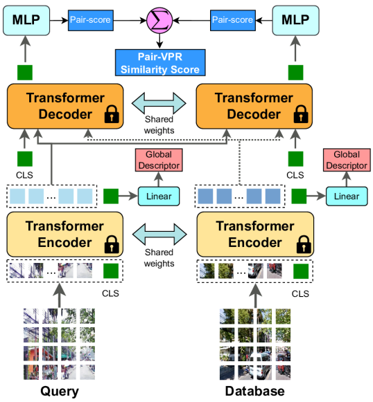
Figure 2: During inference, we are able to pass in pairs of (query, database) images and the network produces a score estimating whether or not the pair of images are from the same location or not, along with a global descriptor per image.

IV Implementation Details

IV-A Stage One Training

We begin by pre-initialising the ViT encoder with weights from DINOv2 [31]. We found that leveraging the diverse pre-training policy used in DINOv2 improved performance over random initialization (please refer to ablation studies in Table II). We then freeze the first half of the encoder blocks (e.g., six blocks with ViT-B) and train the second half using Place-Aware Masked Image Modelling. We train in a Place-aware fashion and construct a dataloader such that a single item in a batch is a single place, where an item comprises a pair of images. We selected three existing large open source datasets for stage one training: SF-XL [17], GSV-Cities [10], and Google Landmarks v2 [18].

SF-XL: We follow the procedure described in EigenPlaces[39] and divide the dataset into $M\times M$ meter-sized cells based on the UTM coordinates of all panoramic images in the dataset, generating a total of $C$ cells. Considering the $i$-th cell $C_{i}$, we follow the approach in EigenPlaces of computing the Singular Value Decomposition (SVD) from the UTM coordinates of all images in this cell, along with the mean UTM coordinate $\mu_{i}$ for this cell. We then select pairs of panoramic images randomly from each cell. Given cell $C_{i}$, we begin by calculating a random focal point (e.g., a target UTM coordinate) that we want our pairs to observe, anchored to the first principle component of the cell denoted as $V_{0}^{i}$. Our formula for calculating a focal point is given below:

$$f_{i}=\mu_{i}+D_{i}\times\textbf{R}\left(V_{0}^{i},O_{i}\right),$$ (5)

where $O_{i}$ is a random observation angle, and $D_{i}$ is a random focal length. At each iteration, we randomly sample observation angles $O_{i}$ between $0$ and $360$ degrees and apply this random rotation to the eigenvector $V_{0}^{i}$. We then randomly sample different focal lengths $D_{i}$, sampling between 10 and 20 meters away from the mean coordinate $\mu_{i}$. This approach differs from the method in EigenPlaces, which only utilized the $0$ and $90$ degree observation angles and a fixed focal length.

Then given a focal point $f_{i}$, we produce crops from two randomly sampled panoramic images within cell $C_{i}$, such that the cropped views are focused on the target focal point - this ensures that our pair of images contains overlapping visual information, without requiring any manual curation of pairs. We can then calculate a viewing angle between a given panoramic image $j$ and a focal point using their respective UTM coordinates:

$$\alpha_{j}=arctan\left(\frac{e_{f}-e_{j}}{n_{f}-n_{j}}\right).$$ (6)

Given this viewing angle, we select a $512$ by $512$ pixel crop from a $3328$ by $512$ pixel panoramic image. However, pairs can be selected that are either too easy (small viewpoint difference), or too hard (too much viewpoint difference). Therefore, we calculate the difference in angles between our two sampled crops:

$$\theta_{i}=\angle\alpha_{1}-\angle\alpha_{2}.$$ (7)

Then we check if $\theta_{i}$ is between a low and high threshold $3$°and $50$°. If not, we resample until we return a pair of crops within the required range.

GSV-Cities: We randomly sample a pair of images from each place in the GSV-Cities dataset, excluding places with less than $4$ images available.

GLDv2: To improve the data diversity, we also added the Google Landmarks dataset [18]. We only use the cleaned subset of the dataset to avoid damaging the network’s ability to learn by providing ambiguous image pairs. Additionally, we also exclude any landmarks with less than $4$ images. We consider a landmark as a proxy for a place and treat the dataset in the same format as SF-XL and GSV-Cities. In total, we are left with $72,322$ landmarks for training after cleaning and filtering.

Training Summary: We merge the three aforementioned datasets to produce a total of $266809$ places per epoch, which are sampled from a set of $3.43$ million panoramic images and $2.08$ million egocentric images. We train using a mask ratio of $90$ percent with a ViT-B sized decoder for $500$ epochs with a learning rate of 2e-4 for a batch size of $512$ places with AdamW and a cosine LR scheduler. We train using square images of size $224$ pixels. By default, we use a ViT-B encoder with $4$ register tokens, however, we note that our approach can also work with larger encoder sizes. Hyperparameters for larger encoders are kept the same except we use 1000 epochs.

IV-B Stage Two Training

We continue training our model using the GSV-Cities dataset [10] following training recipe used in prior works such as MixVPR [23] and SALAD [40]. We train for $10$ epochs using a linear LR scheduler with an initial LR of 8e-5, with a weight decay of 5e-2 and a batch size of $100$ places. We also use square images of size $322$, and freeze all encoder layers except the last six. Our global descriptor has only $512$ dimensions and we heuristically set $w$ (the loss balance term) to $2$. We use MSLS-Val as our validation dataset and take the checkpoint with the highest second-stage Recall@1 as the final trained model.

IV-C Evaluation

We evaluate our method on five commonly used benchmark VPR datasets, with a diverse set of environments. The datasets are: MSLS validation set [41], MSLS challenge set [41], Pittsburgh30k [42], Tokyo247 [43] and Nordland [44] (note that we use the split of Nordland from VPRBench [45], with $2760$ query images). During the evaluation, we resize all images to $322\times 322$ resolution. By default, Pair-VPR uses a ViT-B encoder and uses the top 100 candidates after global descriptor matching - we refer to this as the Speed configuration of Pair-VPR (Pair-VPR-s). We also provide a Performance version of Pair-VPR, which has a ViT-G encoder and uses the top $500$ candidates during pair-classification (Pair-VPR-p). We evaluate using the standard Recall@N metric [6, 17] with $N\in 1,5,10$.

To compare Pair-VPR with existing techniques, we benchmark against five existing single-stage learnt VPR methods (CosPlace [17], MixVPR [23], EigenPlaces [39], BoQ [46] and SALAD [40]) and three existing two-stage VPR techniques (Patch-NetVLAD [12], R2Former [25] and SelaVPR [11]).

V Results and Discussion

TABLE I: Quantitative results for VPR methods on benchmark datasets. Rows above and below the line denote single-stage and two-stage VPR methods respectively. Underlined numbers denote the second best in a column.

Method	Enc. Size	MSLS-Val			MSLS-Challenge			Pitts30k			Tokyo24/7			Nordland
		R@1	R@5	R@10	R@1	R@5	R@10	R@1	R@5	R@10	R@1	R@5	R@10	R@1	R@5	R@10
CosPlace [17]	ResNet-50	87.4	94.1	94.9	67.0	77.9	80.7	90.9	95.7	96.7	87.3	94.0	95.6	55.3	71.5	77.5
MixVPR [23]	ResNet-50	88.0	92.7	94.6	64.0	75.9	80.6	91.5	95.5	96.3	85.1	91.7	94.3	58.4	74.6	80.0
EigenPlaces [39]	ResNet-50	89.1	93.8	95.0	67.4	77.1	81.7	92.5	96.8	97.6	92.4	96.2	97.1	54.4	68.8	74.1
BoQ [46]	ResNet-50	91.2	95.3	96.1	72.8	83.1	86.3	92.4	96.5	97.4	90.5	95.2	96.5	70.7	84.0	87.5
SALAD [40]	ViT-B	92.2	96.4	97.0	75.0	88.8	91.3	92.4	96.3	97.4	95.2	97.1	98.1	76.0	89.2	92.0
Patch-NetVLAD-s [12]	VGG-16	77.3	84.2	86.5	35.8	50.1	55.3	87.1	93.9	95.4	67.6	74.6	77.8	24.8	29.2	30.7
R2Former [25]	ViT-S	89.7	95.0	96.2	73.0	85.9	88.8	91.1	95.2	96.3	88.6	91.4	91.7	-	-	-
SelaVPR [11]	ViT-L	90.8	96.4	97.2	73.5	87.5	90.6	92.8	96.8	97.7	94.0	96.8	97.5	66.2	79.8	84.1
Pair-VPR-s (Ours)	ViT-B	93.7	97.2	97.3	79.0	86.9	88.3	94.7	97.2	97.8	98.1	98.4	98.7	84.2	90.9	91.6
Pair-VPR-p (Ours)	ViT-G	95.4	97.3	97.7	81.7	90.2	91.3	95.4	97.5	98.0	100	100	100	91.0	95.2	95.7

TABLE II: Stage One Training Ablation Study for VPR. Bold denotes the standard configurations of Pair-VPR.

Ablation	Enc. size	Initialization	MSLS-Val			Pitts30k			Tokyo24/7			Nordland
			R@1	R@5	R@10	R@1	R@5	R@10	R@1	R@5	R@10	R@1	R@5	R@10
No stage one training	ViT-B	DINOv2	78.2	95.4	96.1	89.3	95.3	96.5	92.1	97.1	97.8	54.5	74.6	78.6
Training without pairs	ViT-B	DINOv2	91.2	95.0	95.7	91.8	95.8	96.8	93.0	94.9	95.6	67.3	76.4	78.5
Unfreeze all encoder blocks	ViT-B	DINOv2	91.9	96.0	96.8	93.1	96.5	97.2	94.3	95.9	96.2	78.7	86.6	88.3
Train from scratch	ViT-B	Random	88.4	91.5	91.8	92.8	95.8	96.4	83.2	85.4	86.4	42.7	45.9	46.3
Pair-VPR-s (Top100-B)	ViT-B	DINOv2	93.7	97.2	97.3	94.7	97.2	97.8	98.1	98.4	98.7	84.2	90.9	91.6
Pair-VPR (Top100-L)	ViT-L	DINOv2	94.5	97.0	97.4	94.0	97.0	97.8	96.8	96.8	96.8	86.6	91.2	91.5
Pair-VPR (Top100-G)	ViT-G	DINOv2	95.1	97.2	97.6	95.4	97.5	97.9	98.4	98.4	98.4	85.8	89.1	89.4
Pair-VPR-p (Top500-G)	ViT-G	DINOv2	95.4	97.3	97.7	95.4	97.5	98.0	100	100	100	91.0	95.2	95.7

V-A Comparison to Recent VPR Methods

We begin by comparing the performance of Pair-VPR against other State-Of-The-Art (SOTA) VPR methods on a range of benchmark datasets, and we provide both quantitative and qualitative results in Table I and Figure 3 respectively. Comparing our method Pair-VPR-s to the other methods we benchmark, we observe that Pair-VPR achieves the highest Recall@1 on all five datasets. We observe that our transformer-based re-ranking network is particularly adapt at improving the Recall@1 over prior works that also use a vision transformer backbone (SALAD [40] and SelaVPR [11]). Comparing against R2Former [25], which is a prior SOTA method which also used a re-ranking/pair-classifier transformer, we observe a significant jump in performance especially on the Tokyo dataset.

When we scale up our method to use larger encoder sizes and more top candidates, we observe that Pair-VPR-p provides a large performance increase over Pair-VPR-s and achieves the highest recall across all recall@N values compared to prior works. We especially highlight the results on Tokyo24/7, where we have achieved a Recall@1 of $100$%.

V-B Pre-training Ablation Study

To understand which aspects of our training strategy are essential for the performance of Pair-VPR, we conducted an ablation study over different variations of stage one training (Table II). In the first row, we show the results when we don’t perform stage one training at all, with the decoder in stage two initialized using random weights. We observed that pre-training the decoder network via stage one training is essential to achieve effective VPR performance - as the pair-classification task is non-trivial, the place-aware siamese mask image modelling task provides an initial set of weights that are already tuned for comparing features between two images.

In the second row of Table 2, we investigated the importance of place-aware sampling by removing the place sampling during stage one training, and instead used strong augmentation to generate the second unmasked image. We observed a consistent drop in recall, even though the total collection of training images is kept identical.

In row three, we experimented with unfreezing all blocks in our Dinov2 initialized ViT encoder. We found that allowing the entire network to be trained reduced the VPR performance and we hypothesise that this is because the DINOv2 network was originally trained on a larger and more diverse dataset than ours, and maintaining the low level (e.g., color) learnt features from a more diverse dataset improves performance.

In the fourth row we instead initialized the ViT encoder with random weights and performed stage one training from scratch. We found that the VPR performance is still maintained well on urban datasets, but reduces significantly on non-urban datasets like Nordland. This is likely due to the urban bias in common VPR pre-training datasets.

In the bottom four rows, we compared different configurations of Pair-VPR. We observed that the performance of Pair-VPR increases as we increase the encoder size. We further observed that increasing the number of top candidates passed to the pair classification component increases the recall, as it reduces the performance limitation imposed by the effectiveness of the global descriptor.

TABLE III: Performance of the Pair-VPR Global Descriptor (512-dim)

Method	MSLS-Val			Pitts30k			Tokyo24/7
	R@1	R@100	R@500	R@1	R@100	R@500	R@1	R@100	R@500
Pair-VPR-s (Global)	86.4	97.8	98.5	89.3	99.0	99.8	85.1	99.1	99.7
Pair-VPR-s (Refine)	93.7	97.8	97.8	94.7	99.0	99.0	98.1	99.1	99.1
Pair-VPR-p (Global)	86.6	98.4	98.8	90.2	99.1	99.6	77.8	99.1	100
Pair-VPR-p (Refine)	95.4	98.5	98.8	95.4	99.3	99.6	100	100	100

V-C Performance of the Pair-VPR Global Descriptor

In Table III, we analyse the performance of the Pair-VPR global descriptor. The performance of the second stage refinement is always limited by the recall of the global descriptor at the chosen number of top candidates, therefore we display Recall@N values for $N\in 1,100,500$. The global descriptor is always $512$ dimensions, allowing for computationally efficient database searching while also having a Recall@1 comparable to existing global descriptor VPR methods. We also note that our global descriptor is a lot smaller than the single-stage VPR methods in Table I, e.g., CosPlace, MixVPR and SALAD have $2048$, $4096$ and $8448$ dimensions respectively.

When we shift to using larger encoder sizes, we always maintain the same global descriptor by increasing the projection ratio from the class token. For a ViT-G encoder, the class token has $1530$ dimensions and we project down to $512$ dimensions using a linear layer. We do this in order to keep the computational cost of descriptor matching the same. We find that the ViT-G global descriptor performs similar to the ViT-B descriptor, except on Tokyo24/7. It is possible that the large projection ratio is not ideal for VPR, therefore future work should investigate experimenting with larger global descriptor sizes, albeit at an increased compute requirement.

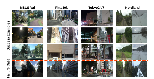
Figure 3: Qualitative results on the benchmark datasets, showing the performance of the computationally cheapest version of Pair-VPR (Pair-VPR-s). We provide three success examples and one failure case per dataset, showing that Pair-VPR can operate even when there is severe viewpoint shift, seasonal changes or at night.

TABLE IV: Compute Analysis of two-stage methods on MSLS-Val

Method	Encoding	Matching	Refinement	Storage
	(ms/query)	(ms/query)	(ms/pair)	(mB/image)
Patch-NetVLAD-s	12.51	0.17	0.94	1.83
Patch-NetVLAD-p	211.0	0.26	32.32	45.22
R2Former	7.11	0.33	0.74	0.25
SelaVPR	9.71	0.08	0.91	0.46
Pair-VPR-s (ViT-B)	7.31	0.13	7.18	1.55
Pair-VPR-p (ViT-G)	33.17	0.13	7.31	3.10

V-D Compute Analysis

In this subsection we discuss the computational requirements of Pair-VPR and compare against other two-stage VPR methods using the same compute platform (a server computer limited to using a single GPU), as shown in Table IV. It can be seen that Pair-VPR-s is fast at encoding and matching, taking $7$ milliseconds per query image to encode and only $0.13$ ms/query to match against the entire database using $512$ dimensional descriptors. Our second stage refinement is slower than SelaVPR and R2Former but much faster than Patch-NetVLAD-p, and requires $0.7$ seconds per query with $100$ top candidates. Comparing the ViT-B to ViT-G encoder sizes of Pair-VPR, only the encoding time and storage requirement increases, since we maintain the same global descriptor size and the same decoder network size. The storage requirements of Pair-VPR are primarily from the dense features required for refinement and Pair-VPR-s features are comparable in size to Patch-NetVLAD-s and SelaVPR.

VI Conclusion

In summary, we present Pair-VPR, a novel two-stage VPR method that relies upon a mask image modelling pre-training strategy to maximise performance. Pair-VPR combines a small $512$ dimensional global descriptor for rapid database searching along with a slower second stage that only searches a set of potential database matches. We observed that Pair-VPR achieved the highest Recall@1 score on all datasets we tested on, comparing against recent state-of-the-art methods in VPR literature - while only requiring an encoder and decoder of $86$ million parameters each. As the encoder size is scaled up to ViT-L ($307$M) and ViT-G ($1.1$B), our training recipe allows for continuing performance improvements as the network size grows. Given the high recalls attained by Pair-VPR, we believe it prudent to investigate converting this method from a VPR technique to a loop closure module in a full SLAM system. In future, we aim to investigate the effectiveness of Pair-VPR at performing loop closures in SLAM.

References

- [1] L. Wiesmann, L. Nunes et al., “Kppr: Exploiting momentum contrast for point cloud-based place recognition,” IEEE Robotics and Automation Letters, vol. 8, no. 2, pp. 592–599, 2022.
- [2] K. Vidanapathirana, M. Ramezani et al., “Logg3d-net: Locally guided global descriptor learning for 3d place recognition,” in 2022 International Conference on Robotics and Automation (ICRA), 2022, pp. 2215–2221.
- [3] G. Peng, H. Li et al., “Transloc4d: Transformer-based 4d radar place recognition,” in Proceedings of the IEEE/CVF Conference on Computer Vision and Pattern Recognition, 2024, pp. 17 595–17 605.
- [4] D. C. Herraez, L. Chang et al., “Spr: Single-scan radar place recognition,” IEEE Robotics and Automation Letters, 2024.
- [5] S. Lowry, N. Sünderhauf et al., “Visual place recognition: A survey,” IEEE Transactions on Robotics, vol. 32, no. 1, pp. 1–19, 2016.
- [6] R. Arandjelović, P. Gronat et al., “NetVLAD: CNN architecture for weakly supervised place recognition,” IEEE Trans. Pattern Anal. Mach. Intell., vol. 40, no. 6, pp. 1437–1451, 2018.
- [7] Z. Chen, A. Jacobson et al., “Deep learning features at scale for visual place recognition,” in 2017 IEEE international conference on robotics and automation (ICRA). IEEE, 2017, pp. 3223–3230.
- [8] H. Jégou, M. Douze et al., “Aggregating local descriptors into a compact image representation,” in 2010 IEEE computer society conference on computer vision and pattern recognition. IEEE, 2010, pp. 3304–3311.
- [9] F. Radenović, G. Tolias, and O. Chum, “Fine-tuning cnn image retrieval with no human annotation,” IEEE transactions on pattern analysis and machine intelligence, vol. 41, no. 7, pp. 1655–1668, 2018.
- [10] A. Ali-bey, B. Chaib-draa, and P. Giguère, “Gsv-cities: Toward appropriate supervised visual place recognition,” Neurocomputing, vol. 513, pp. 194–203, 2022.
- [11] F. Lu, L. Zhang et al., “Towards seamless adaptation of pre-trained models for visual place recognition,” in The Twelfth International Conference on Learning Representations, 2024.
- [12] S. Hausler, S. Garg et al., “Patch-netvlad: Multi-scale fusion of locally-global descriptors for place recognition,” in Proceedings of the IEEE/CVF Conference on Computer Vision and Pattern Recognition, 2021, pp. 14 141–14 152.
- [13] R. Wang, Y. Shen et al., “Transvpr: Transformer-based place recognition with multi-level attention aggregation,” in Proceedings of the IEEE/CVF Conference on Computer Vision and Pattern Recognition, 2022, pp. 13 648–13 657.
- [14] K. Vidanapathirana, P. Moghadam et al., “Spectral geometric verification: Re-ranking point cloud retrieval for metric localization,” IEEE Robotics and Automation Letters, vol. 8, no. 5, pp. 2494–2501, 2023.
- [15] A. Gupta, J. Wu et al., “Siamese masked autoencoders,” Advances in Neural Information Processing Systems, vol. 36, pp. 40 676–40 693, 2023.
- [16] P. Weinzaepfel, V. Leroy et al., “Croco: Self-supervised pre-training for 3d vision tasks by cross-view completion,” Advances in Neural Information Processing Systems, vol. 35, pp. 3502–3516, 2022.
- [17] G. Berton, C. Masone, and B. Caputo, “Rethinking visual geo-localization for large-scale applications,” in Proceedings of the IEEE/CVF Conference on Computer Vision and Pattern Recognition, 2022, pp. 4878–4888.
- [18] T. Weyand, A. Araujo et al., “Google landmarks dataset v2-a large-scale benchmark for instance-level recognition and retrieval,” in Proceedings of the IEEE/CVF conference on computer vision and pattern recognition, 2020, pp. 2575–2584.
- [19] J. Thoma, D. P. Paudel, and L. V. Gool, “Soft contrastive learning for visual localization,” Advances in Neural Information Processing Systems, vol. 33, pp. 11 119–11 130, 2020.
- [20] M. A. Uy and G. H. Lee, “Pointnetvlad: Deep point cloud based retrieval for large-scale place recognition,” in Proceedings of the IEEE conference on computer vision and pattern recognition, 2018, pp. 4470–4479.
- [21] M. Leyva-Vallina, N. Strisciuglio, and N. Petkov, “Data-efficient large scale place recognition with graded similarity supervision,” in Proceedings of the IEEE/CVF Conference on Computer Vision and Pattern Recognition, 2023, pp. 23 487–23 496.
- [22] J. Yu, C. Zhu et al., “Spatial pyramid-enhanced netvlad with weighted triplet loss for place recognition,” IEEE transactions on neural networks and learning systems, vol. 31, no. 2, pp. 661–674, 2019.
- [23] A. Ali-Bey, B. Chaib-Draa, and P. Giguere, “Mixvpr: Feature mixing for visual place recognition,” in Proceedings of the IEEE/CVF Winter Conference on Applications of Computer Vision, 2023, pp. 2998–3007.
- [24] Z. Li, C. D. W. Lee et al., “Hot-netvlad: Learning discriminatory key points for visual place recognition,” IEEE Robotics and Automation Letters, vol. 8, no. 2, pp. 974–980, 2023.
- [25] S. Zhu, L. Yang et al., “R2former: Unified retrieval and reranking transformer for place recognition,” in Proceedings of the IEEE/CVF Conference on Computer Vision and Pattern Recognition, 2023, pp. 19 370–19 380.
- [26] J. Knights, S. Hausler et al., “Geoadapt: Self-supervised test-time adaptation in lidar place recognition using geometric priors,” IEEE Robotics and Automation Letters, vol. 9, no. 1, pp. 915–922, 2024.
- [27] A. Dosovitskiy, L. Beyer et al., “An image is worth 16x16 words: Transformers for image recognition at scale,” in International Conference on Learning Representations, 2021.
- [28] T. Chen, S. Kornblith et al., “A simple framework for contrastive learning of visual representations,” in International conference on machine learning. PMLR, 2020, pp. 1597–1607.
- [29] J.-B. Grill, F. Strub et al., “Bootstrap your own latent-a new approach to self-supervised learning,” Advances in neural information processing systems, vol. 33, pp. 21 271–21 284, 2020.
- [30] M. Caron, H. Touvron et al., “Emerging properties in self-supervised vision transformers,” in Proceedings of the IEEE/CVF international conference on computer vision, 2021, pp. 9650–9660.
- [31] M. Oquab, T. Darcet et al., “DINOv2: Learning robust visual features without supervision,” Transactions on Machine Learning Research, 2024.
- [32] H. Bao, L. Dong et al., “BEit: BERT pre-training of image transformers,” in International Conference on Learning Representations, 2022.
- [33] K. He, X. Chen et al., “Masked autoencoders are scalable vision learners,” in Proceedings of the IEEE/CVF conference on computer vision and pattern recognition, 2022, pp. 16 000–16 009.
- [34] J. Zhou, C. Wei et al., “Image BERT pre-training with online tokenizer,” in International Conference on Learning Representations, 2022.
- [35] M. Haghighat, P. Moghadam et al., “Pre-training with random orthogonal projection image modeling,” in The Twelfth International Conference on Learning Representations, 2024.
- [36] T. Dao, D. Fu et al., “Flashattention: Fast and memory-efficient exact attention with io-awareness,” Advances in Neural Information Processing Systems, vol. 35, pp. 16 344–16 359, 2022.
- [37] K. Musgrave, S. J. Belongie, and S.-N. Lim, “Pytorch metric learning,” ArXiv, vol. abs/2008.09164, 2020.
- [38] X. Wang, X. Han et al., “Multi-similarity loss with general pair weighting for deep metric learning,” in Proceedings of the IEEE/CVF conference on computer vision and pattern recognition, 2019, pp. 5022–5030.
- [39] G. Berton, G. Trivigno et al., “Eigenplaces: Training viewpoint robust models for visual place recognition,” in Proceedings of the IEEE/CVF International Conference on Computer Vision, 2023, pp. 11 080–11 090.
- [40] S. Izquierdo and J. Civera, “Optimal transport aggregation for visual place recognition,” in Proceedings of the IEEE/CVF Conference on Computer Vision and Pattern Recognition, 2024, pp. 17 658–17 668.
- [41] F. Warburg, S. Hauberg et al., “Mapillary street-level sequences: A dataset for lifelong place recognition,” in Proceedings of the IEEE/CVF conference on computer vision and pattern recognition, 2020, pp. 2626–2635.
- [42] A. Torii, J. Sivic et al., “Visual place recognition with repetitive structures,” in Proceedings of the IEEE conference on computer vision and pattern recognition, 2013, pp. 883–890.
- [43] A. Torii, R. Arandjelovic et al., “24/7 place recognition by view synthesis,” in Proceedings of the IEEE conference on computer vision and pattern recognition, 2015, pp. 1808–1817.
- [44] S. Skrede, “Nordlandsbanen: minute by minute, season by season,” 2013.
- [45] M. Zaffar, S. Garg et al., “Vpr-bench: An open-source visual place recognition evaluation framework with quantifiable viewpoint and appearance change,” International Journal of Computer Vision, vol. 129, no. 7, pp. 2136–2174, 2021.
- [46] A. Ali-bey, B. Chaib-draa, and P. Giguère, “Boq: A place is worth a bag of learnable queries,” in Proceedings of the IEEE/CVF Conference on Computer Vision and Pattern Recognition, 2024, pp. 17 794–17 803.