TopoTune: a framework for generalized
combinatorial complex neural networks

Abstract

Graph Neural Networks (GNNs) excel in learning from relational datasets, processing node and edge features in a way that preserves the symmetries of the graph domain. However, many complex systems—such as biological or social networks—involve multiway complex interactions that are more naturally represented by higher-order topological spaces. The emerging field of Topological Deep Learning (TDL) aims to accommodate and leverage these higher-order structures. Combinatorial Complex Neural Networks (CCNNs), fairly general TDL models, have been shown to be more expressive and better performing than GNNs. However, differently from the graph deep learning ecosystem, TDL lacks a principled and standardized framework for easily defining new architectures, restricting its accessibility and applicability. To address this issue, we introduce Generalized CCNNs (GCCNs), a novel simple yet powerful family of TDL models that can be used to systematically transform any (graph) neural network into its TDL counterpart. We prove that GCCNs generalize and subsume CCNNs, while extensive experiments on a diverse class of GCCNs show that these architectures consistently match or outperform CCNNs, often with less model complexity. In an effort to accelerate and democratize TDL, we introduce TopoTune, a lightweight software that allows practitioners to define, build, and train GCCNs with unprecedented flexibility and ease.

1 Introduction

Graph Neural Networks (GNNs) (Scarselli et al., 2008; Corso et al., 2024) have demonstrated remarkable performance in several relational learning tasks by incorporating prior knowledge through graph structures (Kipf & Welling, 2017; Zhang & Chen, 2018). However, constrained by the pairwise nature of graphs, GNNs are limited in their ability to capture and model higher-order interactions—crucial in complex systems like particle physics, social interactions, or biological networks (Lambiotte et al., 2019). Topological Deep Learning (TDL) (Bodnar, 2023) precisely emerged as a framework that naturally encompasses multi-way relationships, leveraging beyond-graph combinatorial topological domains such as simplicial and cell complexes, or hypergraphs (Papillon et al., 2023).

In this context, Hajij et al. (2023; 2024a) have recently introduced combinatorial complexes, fairly general objects that are able to model arbitrary higher-order interactions along with a hierarchical organization among them –hence generalizing (for learning purposes) most of the combinatorial topological domains within TDL, including graphs. The elements of a combinatorial complex are cells, being nodes or groups of nodes, which are categorized by ranks. The simplest cell, a single node, has rank zero. Cells of higher ranks define relationships between nodes: rank one cells are edges, rank two cells are faces, and so on. Hajij et al. (2023) also proposes Combinatorial Complex Neural Networks (CCNNs), machine learning architectures that leverage the versatility of combinatorial complexes to naturally model higher-order interactions. For instance, consider the task of predicting the solubility of a molecule from its structure. GNNs model molecules as graphs, thus considering atoms (nodes) and bonds (edges) (Gilmer et al., 2017). By contrast, CCNNs model molecules as combinatorial complexes, hence considering atoms (nodes, i.e. cells of rank zero), bonds (edges, i.e. cells of rank one), and also important higher-order structures such as rings or functional groups (i.e. cells of rank two) (Battiloro et al., 2024).

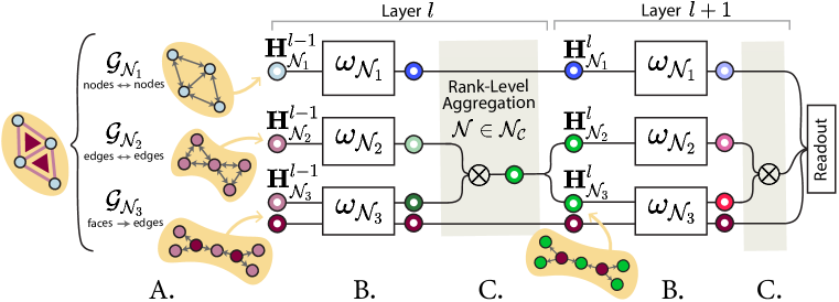
Figure 1: Generalized Combinatorial Complex Network (GCCN). The input complex $\mathcal{C}$ has neighborhoods $\mathcal{N_{C}}=\{\mathcal{N}_{1},\mathcal{N}_{2},\mathcal{N}_{3}$}. A. The complex is expanded into three augmented Hasse graphs $\mathcal{G}_{\mathcal{N}_{i}}$, $i=\{1,2,3\}$, each with features $H_{\mathcal{N}_{i}}$ represented as a colored disc. B. A GCCN layer dedicates one base architecture $\omega_{\mathcal{N}_{i}}$ (GNN, Transformer, MLP, etc.) to each neighborhood. C. The output of all the architectures $\omega_{\mathcal{N}_{i}}$ is aggregated rank-wise, then updated. In this example, only the complex’s edge features (originally pink) are aggregated across multiple neighborhoods ($\mathcal{N}_{2}$ and $\mathcal{N}_{3}$).

TDL Research Trend.

To date, research in TDL has largely progressed by taking existing GNNs architectures (convolutional, attentional, message-passing, etc.) and generalizing them one-by-one to a specific TDL counterpart, whether that be on hypergraphs (Feng et al., 2019; Chen et al., 2020a; Yadati, 2020), on simplicial complexes (Roddenberry et al., 2021; Yang & Isufi, 2023; Ebli et al., 2020; Giusti et al., 2022a; Battiloro et al., 2023; Bodnar et al., 2021b; Maggs et al., 2024), on cell complexes (Hajij et al., 2020; Giusti et al., 2022b; Bodnar et al., 2021a), or on combinatorial complexes (Battiloro et al., 2024; Eitan et al., 2024). Although overall valuable and insightful, such a fragmented research trend is slowing the development of standardized methodologies and software for TDL, as well as limiting the analysis of its cost-benefits trade-offs (Papamarkou et al., 2024). We argue that these two relevant aspects are considerably hindering the use and application of TDL beyond the community of experts.

Current Efforts and Gaps for TDL Standardization.

TopoX (Hajij et al., 2024b) and TopoBenchmark (Telyatnikov et al., 2024) have become the reference Python libraries for developing and benchmarking TDL models, respectively. However, despite their potential in defining and implementing novel standardized methodologies in the field, the current focus of these packages is on replicating and analyzing existing message-passing CCNNs. Works like Jogl et al. (2022b; a) have tackled this problem by porting TDL models to the graph domain via principled transformations from combinatorial topological domains to graphs. However, although these architectures over the resulting graph-expanded representations are as expressive as their TDL counterparts (using the Weisfeiler-Lehman criterion (Xu et al., 2019a)), the former are neither formally equivalent to nor a generalization of the latter. As such, outside of the expressivity side, the GNNs on the resulting graphs cannot be fairly compared with their TDL counterparts.

Contributions. This works seeks to accelerate TDL research and increase its accessibility and standardization for outside practitioners. To that end, we introduce a novel joint methodological and software framework that easily enables the development of new TDL architectures in a principled way—overcoming the limitations of existing works. Our main contributions are as follows:

• Systematic Generalization. We propose the first method to systematically generalize any neural network to its topological counterpart with minimal adaptation. Specifically, we define a novel expansion mechanism that transforms a combinatorial complex into a collection of graphs, enabling the training of TDL models as an ensemble of synchronized models.

• General Architectures. Our method induces a novel wide class of TDL architectures, Generalized Combinatorial Complex Networks (GCCNs), portrayed in Fig. 1. GCCNs (i) formally generalize CCNNs, (ii) are cell permutation equivariant, and (iii) are as expressive as CCNNs.

• Implementation. We provide TopoTune, a lightweight PyTorch module for designing and implementing GCCNs. TopoTune is fully integrated into TopoBenchmark (Telyatnikov et al., 2024). Using TopoTune, both newcomers and expert TDL practitioners can, for the first time, easily define and iterate upon TDL architectures.

• Benchmarking. Using TopoTune, we create a broad class of GCCNs using four base GNNs and one base Transformer over two combinatorial topological spaces (simplicial and cell complexes). A wide range of experiments on graph-level and node-level benchmark datasets shows GCCNs generally outperform existing CCNNs, often with less model complexity. Some of these results are obtained with GCCNs that cannot be reduced to standard CCNNs, further underlining our methodological contribution. We provide all code and experiment scripts through the TopoBenchmark Telyatnikov et al. (2024) repository at github.com/geometric-intelligence/TopoBenchmark.

Outline.

Section 2 provides necessary background. Section 3 motivates and positions our work in the current TDL literature. Section 4 introduces and discusses GCCNs. Section 5 introduces and describes TopoTune. Finally, Section 6 showcases extensive numerical experiments and comparisons.

2 Background

To properly contextualize our work, we revisit in this section the fundamentals of combinatorial complexes and CCNNs—closely following the works of Hajij et al. (2023) and Battiloro et al. (2024)—as well as the notion of augmented Hasse graphs.

Combinatorial Complex.

A combinatorial complex is a triple $(\mathcal{V},\mathcal{C},\textrm{rk})$ consisting of a set $\mathcal{V}$, a subset $\mathcal{C}$ of the powerset $\mathcal{P}(S)\backslash\{\emptyset\}$, and a rank function $\textrm{rk}:\mathcal{C}\rightarrow\mathbb{Z}_{\geq 0}$ with the following properties:

1. for all $v\in\mathcal{V},\{v\}\in\mathcal{C}$ and $\textrm{rk}(\{v\})=0$;

2. the function rk is order-preserving, i.e. if $\sigma,\tau\in\mathcal{C}$ satisfy $\sigma\subseteq\tau$, then $\textrm{rk}(\sigma)\leq$ $\textrm{rk}(\tau)$.

The elements of $\mathcal{V}$ are the nodes, while the elements of $\mathcal{C}$ are called cells (i.e. group of nodes). The rank of a cell $\sigma\in\mathcal{C}$ is $k:=\textrm{rk}(\sigma)$, and we call it a $k$-cell. $\mathcal{C}$ simplifies notation for $(\mathcal{V},\mathcal{C},\textrm{rk})$, and its dimension is defined as the maximal rank among its cell: $\mathrm{dim}(\mathcal{C}):=\max_{\sigma\in\mathcal{C}}\textrm{rk}(\sigma)$.

Neighbhorhoods.

Combinatorial complexes can be equipped with a notion of neighborhood among cells. In particular, a neighborhood $\mathcal{N}:\mathcal{C}\rightarrow\mathcal{P}(\mathcal{C})$ on a CC $\mathcal{C}$ is a function that assigns to each cell $\sigma$ in $\mathcal{C}$ a collection of “neighbor cells" $\mathcal{N}(\sigma)\subset\mathcal{C}\cup\emptyset$. Examples of neighborhood functions are adjacencies, connecting cells with the same rank, and incidences, connecting cells with different consecutive ranks. Usually, up/down incidences $\mathcal{N}_{I,\uparrow}$ and $\mathcal{N}_{I,\downarrow}$ are defined as

$$\mathcal{N}_{I,\uparrow}(\sigma)=\{\tau\in\mathcal{C}\,|\,\textrm{rk}(\tau)=\textrm{rk}(\sigma)+1,\sigma\subset\tau\},\quad\mathcal{N}_{I,\downarrow}(\sigma)=\{\tau\in\mathcal{C}\,|\,\textrm{rk}(\tau)=\textrm{rk}(\sigma)-1,\tau\subset\sigma\}.$$ (1)

Therefore, a $k+1$-cell $\tau$ is a neighbor of a $k$-cell $\sigma$ w.r.t. to $\mathcal{N}_{I,\uparrow}$ if $\sigma$ is contained in $\tau$; analogously, a $k-1$-cell $\tau$ is a neighbor of a $k$-cell $\sigma$ w.r.t. to $\mathcal{N}_{I,\downarrow}$ if $\tau$ is contained in $\sigma$. These incidences induce up/down adjacencies $\mathcal{N}_{A,\uparrow}$ and $\mathcal{N}_{A,\uparrow}$ as

$$\mathcal{N}_{A,\uparrow}(\sigma)=\{\tau\in\mathcal{C}\,|\,\textrm{rk}(\tau)=\textrm{rk}(\sigma),\exists\delta\in\mathcal{C}:\textrm{rk}(\tau)=\textrm{rk}(\sigma)+1,\tau\subset\delta,\text{ and }\sigma\subset\delta\},$$

$$\mathcal{N}_{A,\downarrow}(\sigma)=\{\tau\in\mathcal{C}\,|\,\textrm{rk}(\tau)=\textrm{rk}(\sigma),\exists\delta\in\mathcal{C}:\textrm{rk}(\delta)=\textrm{rk}(\sigma)-1,\delta\subset\tau,\text{ and }\delta\subset\sigma\}.$$ (2)

Therefore, a $k$-cell $\tau$ is a neighbor of a $k$-cell $\sigma$ w.r.t. to $\mathcal{N}_{A,\uparrow}$ if they are both contained in a $k+1$-cell $\delta$; analogously, a $k$-cell $\tau$ is a neighbor of a $k$-cell $\sigma$ w.r.t. to $\mathcal{N}_{A,\downarrow}$ if they both contain a $k-1$-cell $\delta$. Other neighborhood functions can be defined for specific applications (Battiloro et al., 2024).

Combinatorial Complex Message-Passing Neural Networks.

Let $\mathcal{C}$ be a CC, and $\mathcal{N_{C}}$ a collection of neighborhood functions. The $l$-th layer of a CCNN updates the embedding $\mathbf{h}^{l}_{\sigma}\in\mathbb{R}^{F^{l}}$ of cell $\sigma$ as

$$\mathbf{h}_{\sigma}^{l+1}=\phi\left(\mathbf{h}^{l}_{\sigma},\bigotimes_{\mathcal{N}\in\mathcal{N_{C}}}\bigoplus_{\tau\in\mathcal{N}(\sigma)}\psi_{\mathcal{N},\textrm{rk}(\sigma)}\left(\mathbf{h}^{l}_{\sigma},\mathbf{h}^{l}_{\tau}\right)\right)\in\mathbb{R}^{F^{l+1}},$$ (3)

where $\mathbf{h}_{\sigma}^{0}:=\mathbf{h}_{\sigma}$ are the initial features, $\bigoplus$ is an intra-neighborhood aggregator, $\bigotimes$ is an inter-neighborhood aggregator. The rank- and neighborhood-dependent (vector) message functions $\psi_{\mathcal{N},\textrm{rk}(\cdot)}:\mathbb{R}^{F^{l}}\rightarrow\mathbb{R}^{F^{l+1}}$ and the update function $\phi$ are learnable functions. In other words, the embedding of a cell is updated in a learnable fashion by first aggregating messages with neighboring cells per each neighborhood, and then by further aggregating across neighborhoods. We remark that by this definition, all CCNNs are message-passing architectures.

Augmented Hasse Graphs.

Given a collection of neighborhood functions on it, every combinatorial complex $\mathcal{C}$ can be expanded into a unique graph representation, which we refer to as an augmented Hasse graph (Hajij et al., 2023). Formally, let $\mathcal{N_{C}}$ be a collection of neighborhood functions on $\mathcal{C}$: the augmented Hasse graph $\mathcal{G}_{\mathcal{N}_{\mathcal{C}}}$ of $\mathcal{C}$ induced by $\mathcal{N_{C}}$ is a directed graph $\mathcal{G}_{\mathcal{N_{C}}}=$ $\left(\mathcal{C},\mathcal{E}_{\mathcal{N_{C}}}\right)$ with cells as nodes, and edges given by

$$\mathcal{E}_{\mathcal{N_{C}}}=\{(\tau,\sigma)|\sigma,\tau\in\mathcal{C},\exists\ \mathcal{N}\in\mathcal{N_{C}}:\tau\in\mathcal{N}(\sigma)\}.$$ (4)

The augmented Hasse graph of a combinatorial complex is thus obtained by considering the cells as nodes, and inserting directed edges among them if the cells are neighbors in $\mathcal{C}$. Fig. 2 shows an example of a combinatorial complex and an augmented Hasse graph representing it. Notably, all information about cell rank is discarded in this expansion.

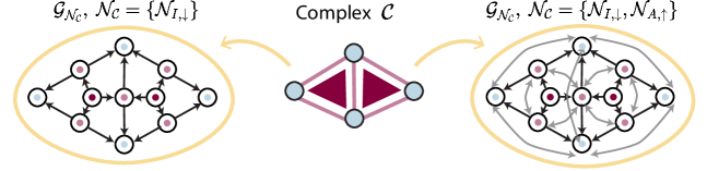
Figure 2: Augmented Hasse graphs. Expansions of a combinatorial complex $\mathcal{C}$ (middle) into two augmented Hasse graphs: (left) the augmented Hasse graph induced by $\mathcal{N}_{\mathcal{C}}=\{\mathcal{N}_{I,\downarrow}\}$; (right) the augmented Hasse graph induced by $\mathcal{N}_{\mathcal{C}}=\{\mathcal{N}_{I,\downarrow},\mathcal{N}_{A,\uparrow}\}$. Information on cell rank is discarded (we retain rank color for illustrative purposes).

3 Motivation

As outlined in the introduction, TDL lacks a comprehensive framework for easily creating and experimenting with novel topological architectures—unlike the more established GNN field. Additionally, a framework of this kind should ensure that its induced architectures retain the expressivity, equivariance, and generality of their TDL counterpart—regardless of the topological domain they are defined onto. This section outlines some previous works that have laid important groundwork in addressing this challenge.

Formalizing CCNNs on graphs.

The position paper (Veličković, 2022) proposed that any function over a higher-order domain can be computed via message passing over a transformed graph, but without specifying how to design GNNs that reproduce CCNNs. Later, (Hajij et al., 2023) proposed that, given a combinatorial complex $\mathcal{C}$ and a collection of neighborhoods $\mathcal{N_{C}}$, a message-passing GNN that runs over the augmented Hasse graph $\mathcal{G}_{\mathcal{N_{C}}}$ is equivalent to a specific CCNN as in (3) running over $\mathcal{C}$ using

• $\mathcal{N_{C}}$ as collection of neighborhoods:

• same intra- and inter-aggregations, i.e., $\bigoplus=\bigotimes$;

• and no rank- and neighborhood-dependent message functions, i.e., $\psi_{\mathcal{N},\textrm{rk}(\cdot)}=\psi\;\forall\mathcal{N}\in\mathcal{N_{C}}$.

Retaining expressivity, but not generality.

The works in (Jogl et al., 2022a; b) show that GNNs over the augmented Hasse graph $\mathcal{G}_{\mathcal{N_{C}}}$ are as expressive (using the WL criterion) as CCNNs over $\mathcal{C}$, i.e., they are equally effective in distinguishing non-isomorphic graphs. These results are appealing because they suggest that some specific CCNNs (as described in eq. 3) can be implemented with standard graph libraries without loss of expressivity. A next work from the same authors generalize these ideas to a wider class of non-standard message-passing GNNs (Jogl et al., 2024). As the authors state, message-passing GNNs over $\mathcal{G}_{\mathcal{N_{C}}}$ cannot model all CCNNs over $\mathcal{C}$ because they do not explicitly differentiate among neighborhoods and cells of different ranks. Therefore, GNNs over augmented Hasse graphs cannot be exhaustively used as surrogates of CCNNs, if not on the expressivity side. Moreover, these works focus on leveraging graph expansion to simulate existing CCNNs rather than to explore new architectures.

The Particular Case of Hypergraphs.

Hypergraph neural networks have long relied on graph expansions (Telyatnikov et al., 2023), which has allowed the field to leverage advances in the graph domain and, by extension, a much wider breadth of models (Papillon et al., 2023). Most hypergraph models are expanded into graphs using the star (Zhou et al., 2006; Solé et al., 1996), the clique (Bolla, 1993; Rodríguez, 2002; Gibson et al., 2000), or the line expansion (Bandyopadhyay et al., 2020). As noted by Agarwal et al. (2006), many hypergraph learning algorithms in fact correspond to either the clique or star expansions with an appropriate weighting function. Further implementations are well captured in the survey (Antelmi et al., 2023).

The success story of hypergraph neural networks motivates further research on new graph-based expansions that generalize and subsume current CCNNs. These expansions could go beyond augmented Hasse graphs to, at the same time, encompass current CCNNs and exploit progress in the GNN field. Therefore, returning to our core goal of accelerating and democratizing TDL while preserving its theoretical properties, we propose a two-part approach: a novel graph-based methodology able to generate general architectures (Section 4), and a lightweight software framework to easily and widely implement it (Section 5).

4 Generalized Combinatorial Complex Neural Networks

We propose Generalized Combinatorial Complex Neural Networks (GCCNs), a novel broad class of TDL architecture. GCCNs overcome the limitations of previous graph-based TDL architectures by leveraging the notions of strictly augmented Hasse graphs and per-rank neighborhoods.

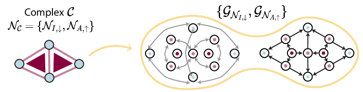
Figure 3: Ensemble of strictly augmented Hasse Graphs. Given a complex $\mathcal{C}$ with neighborhood structure including both incidence and upper adjacency (left), this graph projection (right) produces one augmented Hasse graph for each neighborhood.

Ensemble of Strictly Augmented Hasse Graphs.

This graph expansion method (see Fig. 3) extends from the the established definition of an augmented Hasse graph (see Fig. 2). Specifically, given a combinatorial complex $\mathcal{C}$ and a collection of neighborhood functions $\mathcal{N_{C}}$, we expand it into $|\mathcal{N_{C}}|$ graphs, each of them representing a neighborhood $\mathcal{N}\in\mathcal{N}_{\mathcal{C}}$. In particular, the strictly augmented Hasse graph $\mathcal{G}_{\mathcal{N}}=(\mathcal{C}_{\mathcal{N}},\mathcal{E}_{\mathcal{N}})$ of a neighborhood $\mathcal{N}\in\mathcal{N}_{\mathcal{C}}$ is a directed graph whose nodes $\mathcal{C}_{\mathcal{N}}$ and edges $\mathcal{E}_{\mathcal{N}}$ are given by:

$$\mathcal{C}_{\mathcal{N}}=\{\sigma\in\mathcal{C}\,|\,\mathcal{N}(\sigma)\neq\emptyset\},\;\mathcal{E}_{\mathcal{N}}=\{(\tau,\sigma)\,|\,\tau\in\mathcal{N}(\sigma)\}.$$ (5)

Following the same arguments from Hajij et al. (2023), a GNN over the strictly augmented Hasse graph $\mathcal{G}_{\mathcal{N}}$ induced by $\mathcal{N}$ is equivalent to a CCNN running over $\mathcal{C}$ and using $\mathcal{N_{C}}=\{\mathcal{N}\}$ up to the (self-)update of the cells in $\mathcal{C}/\mathcal{C}_{\mathcal{N}}$.

Per-rank Neighborhoods.

The standard definition of adjacencies and incidences given in Section 2 implies that they are applied to each cell regardless of its rank. For instance, consider a combinatorial complex of dimension two with nodes (0-cells), edges (1-cells), and faces (2-cells).

• Employing the down incidence $\mathcal{N}_{I,\downarrow}$ as in (1) means the edges must exchange messages with their endpoint nodes, and faces must exchange messages with the edges on their sides. It is impossible for edges to exchange messages while faces do not.

• Employing the up adjacency $\mathcal{N}_{A,\uparrow}$ as in (2) means the nodes must exchange messages with other edge-connected nodes, and edges must exchange messages the other edges bounding the same faces. It is impossible for nodes to exchange messages while edges do not.

This limitation increases the computational burden of standard CCNNs while not always increasing the learning performance, as we will show in the numerical results. For this reason, we introduce per-rank neighborhoods, depicted in Fig. 4. Formally, a per-rank neighborhood function $\mathcal{N}^{r}$ is a neighborhood function that, regardless of its definition, maps a cell $\sigma$ to the the empty set if $\sigma$ is not a $r$-cell (i.e., a cell of rank $r$). For example, the up/down $r$-incidences $\mathcal{N}^{r}_{I,\uparrow}$ and $\mathcal{N}^{r}_{I,\downarrow}$ are defined as

$$\mathcal{N}^{r}_{I,\uparrow}(\sigma)=\left\{\begin{aligned} &\{\tau\in\mathcal{C}\,|\,\textrm{rk}(\tau)=\textrm{rk}(\sigma)+1,\sigma\subset\tau\}\textrm{ if rk}(\sigma)=r\\ &\emptyset\textrm{ otherwise}\end{aligned}\right.,$$ (6)

$$\mathcal{N}^{r}_{I,\downarrow}(\sigma)=\left\{\begin{aligned} &\{\tau\in\mathcal{C}\,|\,\textrm{rk}(\tau)=\textrm{rk}(\sigma)-1,\sigma\subset\tau\}\textrm{ if rk}(\sigma)=r\\ &\emptyset\textrm{ otherwise}\end{aligned}\right.,$$ (7)

and the up/down $r$-adjacencies $\mathcal{N}^{r}_{A,\uparrow}$ and $\mathcal{N}^{r}_{A,\downarrow}$ can be obtained analogously. So, returning to our previous example of a 2-dimensional complex, it is now straightforward to model a setting in which:

• Employing only $\mathcal{N}^{1}_{I,\downarrow}$ (Fig. 4(iii)) allows edges to exchange messages with their bounding nodes but not triangles with their bounding edges.

• Employing only $\mathcal{N}^{0}_{A,\uparrow}$ (Fig. 4(i)) allows nodes to exchange messages with their edge-connected nodes but not edges do not exchange messages with other edges that are part of their same faces.

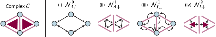
Figure 4: Per-rank neighborhoods. Given a complex $\mathcal{C}$ (left), we illustrate four examples of per-rank neighborhoods (right). In each case, they only include rank-specific cells.

Generating Graph-based TDL Architectures.

We use these notions to define a novel graph-based methodology for generating principled TDL architectures. Given a combinatorial complex $\mathcal{C}$ and a set $\mathcal{N_{C}}$ of neighborhoods, the method works as follows (see also Fig. 1):

1. $\mathcal{C}$ is expanded into an ensemble of strictly augmented Hasse graphs—one for each $\mathcal{N}\in\mathcal{N}_{\mathcal{C}}$.

2. Each strictly augmented Hasse graph $\mathcal{G}_{\mathcal{N}}$ and the features of its cells are independently processed by a base model.

3. An aggregation module $\bigotimes$ synchronizes the cell features across the different strictly augmented Hasse graphs (as the same cells can belong to multiple strictly augmented Hasse graphs).

This method enables an ensemble of synchronized models per layer— the $\omega_{\mathcal{N}}$s—each of them applied to a specific strictly augmented Hasse graph.. Additionally, such a pipeline confers unprecedented flexibility in choosing a subset of neighborhoods of interest, allowing the consideration of per-rank neighborhoods within TDL. The rest of this section formalizes the architectures induced by this methodology and describes their theoretical properties.

Generalized Combinatorial Complex Networks.

We formally introduce a broad class of novel TDL architectures called Generalized Combinatorial Complex Networks (GCCNs), depicted in Fig. 1. Let $\mathcal{C}$ be a combinatorial complex containing $|\mathcal{C}|$ cells and $\mathcal{N_{C}}$ a collection of neighborhoods on it. Assume an arbitrary labeling of the cells in the complex, and denote the $i$-th cell with $\sigma_{i}$. Denote by $\mathbf{H}\in\mathbb{R}^{|\mathcal{C}|\times F}$ the feature matrix collecting some embeddings of the cells on its rows, i.e., $[\mathbf{H}]_{i}=\mathbf{h}_{\sigma_{i}}$, and by $\mathbf{H}_{\mathcal{N}}\in\mathbb{R}^{|\mathcal{C}_{\mathcal{N}}|\times F}$ the submatrix containing just the embeddings of the cells belonging to the strictly augmented Hasse graph $\mathcal{G}_{\mathcal{N}}$ of $\mathcal{N}$. The $l$-th layer of a GCCN updates the embeddings of the cells $\mathbf{H}^{l}\in\mathbb{R}^{|\mathcal{C}|\times F^{l}}$ as

$$\mathbf{H}^{l+1}=\phi\left(\mathbf{H}^{l},\bigotimes_{\mathcal{N}\in\mathcal{N_{C}}}\omega_{\mathcal{N}}(\mathbf{H}^{l}_{\mathcal{N}},\mathcal{G}_{\mathcal{N}})\right)\in\mathbb{R}^{|\mathcal{C}|\times F^{l+1}},$$ (8)

where $\mathbf{H}^{0}$ collects the initial features, and the update function $\phi$ is a learnable row-wise update function, i.e. $[\phi(\mathbf{A},\mathbf{B})]_{i}=\phi([\mathbf{A}]_{i},[\mathbf{B}]_{i})$. The neighborhood-dependent sub-module $\omega_{\mathcal{N}}:\mathbb{R}^{|\mathcal{C}_{\mathcal{N}}|\times F^{l}}\rightarrow\mathbb{R}^{|\mathcal{C}_{\mathcal{N}}|\times F^{l+1}}$, which we refer to as the neighborhood message function, is a learnable (matrix) function that takes as input the whole strictly augmented Hasse graph of the neighborhood, $\mathcal{G}_{\mathcal{N}}$ and the embeddings of the cells that are part of it, and gives as output a processed version of them. Finally, the inter-neighborhood aggregation module $\bigotimes$ synchronizes the possibly multiple neighborhood messages arriving on a single cell across multiple strictly augmented Hasse graphs into a single message. In this way, the embedding of a cell collects information about the whole relational structures induced by each (nonempty) neighborhood.

Given Proposition 1, GCCNs allow us to define general TDL models using any neighborhood message function $\omega_{\mathcal{N}}$, such as any GNN. Not only does this framework avoid having to approximate CCNN computations, as is the case in previous works (Jogl et al., 2022b; a; 2023), but it also enjoys the same permutation equivariance as regular CCNNs (Proposition 2). Differently from the work in (Hajij et al., 2023), the fact that GCCNs can have arbitrary neighborhood message functions implies that non message-passing TDL models can be readily defined (e.g., by using non message-passing models as neighborhood message functions). Moreover, the fact that the whole strictly augmented Hasse graphs are given as input enables also the usage of multi-layer GNNs as neighborhood message functions. To the best of our knowledge, GCCNs are the only objects in the literature that encompass all the above properties.

5 TopoTune

Our proposed methodology, together with its resulting GCCNs architectures, addresses the challenge of systematically generating principled, general TDL models. Here, we introduce TopoTune, a software module for defining and benchmarking GCCN architectures on the fly—a vehicle for accelerating and democratizing TDL research. TopoTune is made available as part of TopoBenchmark Telyatnikov et al. (2024) at github.com/geometric-intelligence/TopoBenchmark. This section details TopoTune’s main features.

Change of Paradigm.

TopoTune introduces a new perspective on TDL through the concept of "neighborhoods of interest," enabling unprecedented flexibility in architectural design. Previously "fixed" components of CCNNs become hyperparameters of our framework. Even the choice of topological domain becomes a mere variable, representing a new paradigm in the design and implementation of TDL architectures.

Accessible TDL.

Using TopoTune, a practitioner can instantiate customized GCCNs simply by modifying a few lines of a configuration file. In fact, it is sufficient to specify $(i)$ a collection of per-rank neighborhoods $\mathcal{N}_{\mathcal{C}}$, $(ii)$ a neighborhood message function $\omega_{\mathcal{N}}$, and optionally $(iii)$ some architectural parameters—e.g. the number $l$ of GCCN layers. For the neighborhood message function $\omega_{\mathcal{N}}$, the same configuration file enables direct import of models from standard PyTorch libraries, including PyTorch Geometric (Fey & Lenssen, 2019) and Deep Graph Library (Chen et al., 2020b). TopoTune’s simplicity provides both newcomers and TDL experts with an accessible tool for defining higher-order topological architectures.

Accelerating TDL Research.

TopoTune is fully integrated into TopoBenchmark (Telyatnikov et al., 2024). This package provides standardized methods for handling combinatorial complex objects, including lifting procedures to lift them from graph-based data. TopoBenchmark also simplifies the training and benchmarking of GCCNs, offering a variety of ready-to-use tasks, datasets, and evaluation metrics. Together, TopoTune and TopoBenchmark provide all the necessary tools to define, train, test, and compare a wide range of novel GCCN architectures, bringing unprecedented versatility and standardization to accelerate TDL research.

6 Experiments

We present experiments showcasing a broad class of GCCN’s constructed with TopoTune. These models consistently match, outperform, or improve upon existing CCNNs, often with smaller model sizes. TopoTune’s integration into the TopoBenchmark experiment infrastructure ensures a fair comparison with CCNNs from the literature, as implementations of data processing, domain lifting, and training are homogeonized. Moreover, TopoBenchmark aggregates TDL’s leading open-source models from TopoX Hajij et al. (2024b), making it an ideal framework for objectively evaluating GCCNs against the current state of the field.

6.1 Experimental Setup

We generate our library by considering ten possible choices of neighborhood structure $\mathcal{N}_{\mathcal{C}}$ (including both regular and per-rank, see Appendix C.1) and five possible choices of $\omega_{\mathcal{N}}$: GCN (Kipf & Welling, 2017), GAT (Velickovic et al., 2017), GIN (Xu et al., 2019b), GraphSAGE (Hamilton et al., 2017), and Transformer (Vaswani et al., 2017). We import these models directly from PyTorch Geometric (Fey & Lenssen, 2019) and PyTorch Paszke et al. (2019). TopoTune enables running GCCNs on both graph expansions previously discussed: an ensemble of strictly augmented Hasse graphs (eq. 5) and a single augmented Hasse graph (eq. 4). In the latter case, each GCCN layer simply contains a single $\omega_{\mathcal{N}}$ (e.g. GNN or Transformer) which processes the single augmented Hasse graph.

Datasets.

We include a wide range of tasks (see Appendix C.2). MUTAG, PROTEINS, NCI01, and NCI09 (Morris et al., 2020) are graph-level classification tasks which seek to predict some property about molecules or proteins. ZINC (Irwin et al., 2012) aims to predict a graph-level property related to molecular solubility through regression. At the node level, the Cora, CiteSeer, and PubMed tasks (Yang et al., 2016) involve classifying publications (nodes) within citation networks. We consider two particular cases of combinatorial complexes, simplicial and cellular complexes, leveraging TopoBenchmark’s data lifting processes to infer higher-order relationships in these datasets (see Appendix C.2 for further details).

6.2 Results and Discussion

Table 1: Cross-domain, cross-task, cross-expansion, and cross-$\omega_{\mathcal{N}}$ comparison of GCCN architectures with top-performing CCNNs benchmarked on TopoBenchmark (Telyatnikov et al., 2024). Best result is in bold and results within 1 standard deviation are highlighted blue. Experiments are run with 5 seeds. We report accuracy for classification tasks and MAE for regression.

	Graph-Level Tasks					Node-Level Tasks
Model	MUTAG ($\uparrow$)	PROTEINS ($\uparrow$)	NCI1 ($\uparrow$)	NCI109 ($\uparrow$)	ZINC ($\downarrow$)	Cora ($\uparrow$)	Citeseer ($\uparrow$)	PubMed ($\uparrow$)
Cellular
CCNN (Best Model on TopoBenchmark)	80.43 ± 1.78	76.13 ± 2.70	76.67 ± 1.48	75.35 ± 1.50	0.34 ± 0.01	87.44 ± 1.28	75.63 ± 1.58	88.64 ± 0.36
GCCN $\omega_{\mathcal{N}}$ = GAT	83.40 ± 4.85	74.05 ± 2.16	76.11 ± 1.69	75.62 ± 0.76	0.38 ± 0.03	88.39 ± 0.65	74.62 ± 1.95	87.68 ± 0.33
GCCN $\omega_{\mathcal{N}}$ = GCN	85.11 ± 6.73	74.41 ± 1.77	76.42 ± 1.67	75.62 ± 0.94	0.36 ± 0.01	88.51 ± 0.70	75.41 ± 2.00	88.18 ± 0.26
GCCN $\omega_{\mathcal{N}}$ = GIN	86.38 ± 6.49	72.54 ± 3.07	77.65 ± 1.11	77.19 ± 0.21	0.19 ± 0.00	87.42 ± 1.85	75.13 ± 1.17	88.47 ± 0.27
GCCN $\omega_{\mathcal{N}}$ = GraphSAGE	85.53 ± 6.80	73.62 ± 2.72	78.23 ± 1.47	77.10 ± 0.83	0.24 ± 0.00	88.57 ± 0.58	75.89 ± 1.84	89.40 ± 0.57
GCCN $\omega_{\mathcal{N}}$ = Transformer	83.83 ± 6.49	70.97 ± 4.06	73.00 ± 1.37	73.20 ± 1.05	0.45 ± 0.02	84.61 ± 1.32	75.05 ± 1.67	88.37 ± 0.22
GCCN $\omega_{\mathcal{N}}$ = Best GNN, 1 Aug. Hasse graph	85.96 ± 7.15	73.73 ± 2.95	76.75 ± 1.63	76.94 ± 0.82	0.31 ± 0.01	87.24 ± 0.58	74.26 ± 1.47	88.65 ± 0.55
Simplicial
CCNN (Best Model on TopoBenchmark)	76.17 ± 6.63	75.27 ± 2.14	76.60 ± 1.75	77.12 ± 1.07	0.36 ± 0.02	82.27 ± 1.34	71.24 ± 1.68	88.72 ± 0.50
GCCN $\omega_{\mathcal{N}}$ = GAT	79.15 ± 4.09	74.62 ± 1.95	74.86 ± 1.42	74.81 ± 1.14	0.57 ± 0.03	88.33 ± 0.67	74.65 ± 1.93	87.72 ± 0.36
GCCN $\omega_{\mathcal{N}}$ = GCN	74.04 ± 8.30	74.91 ± 2.51	74.20 ± 2.17	74.13 ± 0.53	0.53 ± 0.05	88.51 ± 0.70	75.41 ± 2.00	88.19 ± 0.24
GCCN $\omega_{\mathcal{N}}$ = GIN	85.96 ± 4.66	72.83 ± 2.72	76.67 ± 1.62	75.76 ± 1.28	0.35 ± 0.01	87.27 ± 1.63	75.05 ± 1.27	88.54 ± 0.21
GCCN $\omega_{\mathcal{N}}$ = GraphSAGE	75.74 ± 2.43	74.70 ± 3.10	76.85 ± 1.50	75.64 ± 1.94	0.50 ± 0.02	88.57 ± 0.59	75.92 ± 1.85	89.34 ± 0.39
GCCN $\omega_{\mathcal{N}}$ = Transformer	74.04 ± 4.09	70.97 ± 4.06	70.39 ± 0.96	69.99 ± 1.13	0.64 ± 0.01	84.4 ± 1.16	74.6 ± 1.88	88.55 ± 0.39
GCCN $\omega_{\mathcal{N}}$ = Best GNN, 1 Aug. Hasse graph	74.04 ± 5.51	74.48 ± 1.89	75.02 ± 2.24	73.91 ± 3.9	0.56 ± 0.02	87.56 ± 0.66	74.5 ± 1.61	88.61 ± 0.27
Hypergraph
CCNN (Best Model on TopoBenchmark)	80.43 ± 4.09	76.63 ± 1.74	75.18 ± 1.24	74.93 ± 2.50	0.51 ± 0.01	88.92 ± 0.44	74.93 ± 1.39	89.62 ± 0.25

GCCNs outperform CCNNs.

Table 1 portrays a cross-comparison between top-performing CCNN models and our class of GCCNs. GCCNs outperform CCNNs in the simplicial and cellular domains across all datasets. Notably, GCCNs in these domains achieve comparable results to hypergraph CCNNs, a feat unattainable by existing CCNNs in node-level tasks. Moreover, we find both of GCCN’s underlying notions (see Section 4) to be advantageous: (i) Table 1 shows that representing a complex as an ensemble of augmented Hasse graphs consistently yields better performance than using a single augmented Hasse graph. (ii) Some GCCNs with a per-rank neighborhood structure outperform not only CCNNs but also all other GCCNs using regular neighborhoods. For example, this is the case for a cellular GCCN with $\omega_{\mathcal{N}}$ on MUTAG. Its lightweight, per-rank neighborhood structure makes it 19% the size of the best cellular CCNN on this task.

GCCNs are smaller than CCNNs.

GCCNs are generally more parameter efficient than existing CCNNs in simplicial and cellular domains, and in some instances (MUTAG, NCI1, NCI09), even surpass hypergraph CCNNs in size efficiency. Even as GCCNs become more resource-intensive for large graphs with high-dimensional embeddings—as seen in node-level tasks—they maintain a competitive edge. For instance, on the Citeseer dataset, a GCCN ($\omega_{\mathcal{N}}$ = GraphSAGE) outperforms the best existing CCNN while being 28% smaller. We refer to Table 4 in Appendix D.

GCCNs improve existing CCNNs.

TopoTune makes it easy to iterate upon and improve preexisting CCNNs by replicating their architecture in a GCCN setting. For example, TopoTune can generate a counterpart GCCN by replicating a CCNN’s neighborhood structure, aggregation, and training scheme. We show in Table 2 that counterpart GCCNs often achieve comparable or better results than SCCN (Yang et al., 2022) and CWN (Bodnar et al., 2021a) just by sweeping over additional choices of $\omega_{\mathcal{N}}$ (same as in Table 1) available in PyTorch Geometric (Fey & Lenssen, 2019). In the single augmented Hasse graph regime, GCCN models are consistently more lightweight, up to half their size (see Table 5 in Appendix D for details).

Table 2: We compare existing CCNNs with $\omega_{\mathcal{N}}$-modified GCCN counterparts. We show the result for best choice of $\omega_{\mathcal{N}}$. Experiments are run with 5 seeds.

Model	MUTAG	PROTEINS	NCI1	NCI109	Cora	Citeseer	PubMed
SCCN Yang et al. (2022)
Benchmark results Telyatnikov et al. (2024)	70.64 ± 5.90	74.19 ± 2.86	76.60 ± 1.75	77.12 ± 1.07	82.19 ± 1.07	69.60 ± 1.83	88.18 ± 0.32
GCCN, on ensemble of strictly aug. Hasse graphs	82.13 ± 4.66	75.56 ± 2.48	75.6 ± 1.28	74.19 ± 1.44	88.06 ± 0.93	74.67 ± 1.24	87.70 ± 0.19
GCCN, on 1 aug. Hasse graph	69.79 ± 4.85	74.48 ± 2.67	74.63 ± 1.76	70.71 ± 5.50	87.62 ± 1.62	74.86 ± 1.7	87.80 ± 0.28
CWN Bodnar et al. (2021a)
Benchmark results Telyatnikov et al. (2024)	80.43 ± 1.78	76.13 ± 2.70	73.93 ± 1.87	73.80 ± 2.06	86.32 ± 1.38	75.20 ± 1.82	88.64 ± 0.36
GCCN, on ensemble of strictly aug. Hasse graphs	84.26 ± 8.19	75.91 ± 2.75	73.87 ± 1.10	73.75 ± 0.49	85.64 ± 1.38	74.89 ± 1.45	88.40 ± 0.46
GCCN, on 1 aug. Hasse graph	81.70 ± 5.34	75.05 ± 2.39	75.14 ± 0.76	75.39 ± 1.01	86.44 ± 1.33	74.45 ± 1.59	88.56 ± 0.55

Performance-Cost Tradeoff.

By easily sweeping over a wide landscape of possible GCCNs for a given task, TopoTune can help identify “lottery-ticket" models that maximize performance while minimizing computational cost. Fig. 5 illustrates this concept by comparing the performance and size of selected GCCNs across three datasets (see Appendix E for plots on all datasets). On the PROTEINS dataset, two GCCNs using per-rank neighborhood structures (orange and purple) achieve performance within 2% of the best result, while using as little as 48% of the parameters. Similarly, on ZINC, lightweight neighborhood structures (orange and dark green) deliver strong results with reduced parameter costs. We remark that node-level tasks do not always benefit from this parameter reduction. For instance, Citeseer maintains a large model size regardless of neighborhood structure, primarily due to its large graph size and high-dimensional input features. Fig. 5 also provides insights into the impact of neighborhood message functions. On ZINC, GIN clearly outperforms all other models. In less clear-cut cases, we observe a trade-off between neighborhood structure and message function complexity. While GIN and GraphSAGE are generally more parameter-intensive than GAT and GCN, we find that more complex base models on lightweight neighborhood structures perform comparably to simpler base models on more complete neighborhood structures.

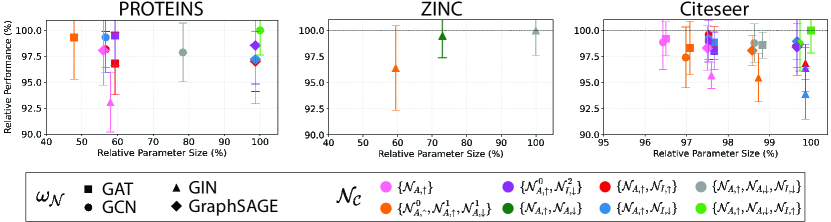
Figure 5: GCCN task-specific performance versus size. We compare relative performance and parameter size of various GCCNs across three datasets on the cellular domain, two graph-level (left, middle) and one node-level (right). Each point represents a different combination of neighborhood structure $\mathcal{N}_{\mathcal{C}}$ and message function $\omega_{\mathcal{N}}$. The amount of layers is kept constant according to the best performing model. Both the x-axis and y-axis are scaled relative to the best performing model.

7 Conclusion

This work introduces a simple yet powerful graph-based methodology for constructing Generalized Combinatorial Complex Neural Networks (GCCNs), TDL architectures that generalize and subsume standard CCNNs. Additionally, we introduce TopoTune, the first lightweight software module for systematically and easily implementing new TDL architectures, all the while leveraging existing GNN (or any other models’) software. Building upon this foundation, we envision several promising directions for future research. Application-specific TDL could seek to customize GCCNs for potentially sparse or multimodal datasets. Additionally, TopoTune’s graph-based approach paves the way for extending state-of-the-art GNN architectures beyond those currently implemented in open-source libraries such as PyTorch Geometric. We hope TopoTune will not only accelerate TDL research but also help bridge the gap with other machine learning fields.

Appendix A Proofs

A.1 Proof of Generality

The proof is trivial. It is sufficient to set $\omega_{\mathcal{N}}(\mathbf{H}^{l}_{\mathcal{N}},\mathcal{G}_{\mathcal{N}})$ to $\{\bigoplus_{y\in\mathcal{N}(\sigma)}\psi_{\mathcal{N},\textrm{rk}(\sigma)}\left(\mathbf{h}^{l}_{\sigma},\mathbf{h}^{l}_{\tau}\right)\}_{\sigma\in\mathcal{C}}$ in (8) as all $y\in\mathcal{N}(\sigma)$ are part of the node set $\mathcal{C}_{\mathcal{N}}$ of the strictly augmented Hasse graph of $\mathcal{N}$ by definition.

A.2 Proof of Equivariance

As for GNNs, an amenable property for GCCNNs is the awareness w.r.t. relabeling of the cells. In other words, given that the order in which the cells are presented to the networks is arbitrary -because CCs, like (undirected) graphs, are purely combinatorial objects-, one would expect that if the order changes, the output changes accordingly. To formalize this concept, we need the following notions.

Matrix Representation of a Neighborhood. Assume again to have a combinatorial complex $\mathcal{C}$ containing $C:=|\mathcal{C}|$ cells and a neighborhood function $\mathcal{N}$ on it. Assume again to give an arbitrary labeling to the cells in the complex, and denote the $i$-th cell with $\sigma_{i}$. The matrix representation of the neighborhood function is a matrix $\mathbf{N}_{\mathcal{N}}\in\mathbb{R}^{C\times C}$ such that $\mathbf{N}_{i,j}=1$ if the $\sigma_{j}\in\mathcal{N}(\sigma_{i})$ or zero otherwise. We notice that the submatrix $\widetilde{\mathbf{N}}_{\mathcal{N}}\in\mathbb{R}^{|\mathcal{C}_{\mathcal{N}}|\times|\mathcal{C}_{\mathcal{N}}|}$ obtained by removing all the zero rows and columns is the adjacency matrix of the strictly augmented Hasse graph $\mathcal{G}_{\mathcal{C}_{\mathcal{N}}}$ induced by $\mathcal{N}$.

Permutation Equivariance. Let $\mathcal{C}$ be combinatorial complex, $\mathcal{N}_{\mathcal{C}}$ a collection of neighborhoods on it, and $\mathbf{N}=\{\mathbf{N}_{\mathcal{N}}\}_{\mathcal{N}\in\mathcal{N}_{\mathcal{C}}}$ the set collecting the corresponding neighborhood matrices. Let $\mathbf{P}\in\mathbb{R}^{C\times C}$ be a permutation matrix. Finally, denote by $\mathbf{PH}$ the permuted embeddings and by $\{\mathbf{PN}_{\mathcal{N}}\mathbf{P}^{T}\}_{\mathcal{N}\in\mathcal{N}_{\mathcal{C}}}$, the permuted neighborhood matrices. We say that a function $f$ : $\left(\mathbf{H}^{l},\mathbf{B}\right)\mapsto\mathbf{H}^{l+1}$ is cell permutation equivariant if $f\left(\mathbf{PH}^{l},\{\mathbf{PN}_{\mathcal{N}}\mathbf{P}^{T}\}_{\mathcal{N}\in\mathcal{N}_{\mathcal{C}}}\right)=\mathbf{P}f\left(\mathbf{H}^{l},\{\mathbf{N}_{\mathcal{N}}\}_{\mathcal{N}\in\mathcal{N}_{\mathcal{C}}}\right)$ for any permutation matrix $\mathbf{P}$. Intuitively, the permutation matrix changes the arbitrary labeling of the cells, and a permutation equivariant function is a function that reflects the change in its output.

Proof of Proposition 2. We follow the approach from (Bodnar et al., 2021a). Given any permutation matrix $\mathbf{P}$, for a cell $\sigma_{i}$, let us denote its permutation as $\sigma_{\mathbf{P}(i)}$ with an abuse of notation. Let $\mathbf{h}^{l+1}_{\sigma_{i}}$ be the output embedding of cell $\sigma_{i}$ for the $l$-th layer of a GCCN taking $(\mathbf{H}^{l},\{\mathbf{N}_{\mathcal{N}}\}_{\mathcal{N}\in\mathcal{N}_{\mathcal{C}}})$ as input, and $\mathbf{h}^{l+1}_{\sigma_{\mathbf{P}(i)}}$ be the output embedding of cell $\sigma_{\mathbf{P}(i)}$ for the same GCCN layer taking $\left(\mathbf{P}\mathbf{H}^{l},\{\mathbf{PN}_{\mathcal{N}}\mathbf{P}^{T}\}_{\mathcal{N}\in\mathcal{N}_{\mathcal{C}}}\right)$ as input. To prove the permutation equivariance, it is sufficient to show that $\mathbf{h}^{l+1}_{\sigma_{i}}=\mathbf{h}^{l+1}_{\sigma_{\mathbf{P}(i)}}$ a the update function $\phi$ is row-wise, i.e. it independetly act on each cell. To do so, we show that the (multi-)set of embeddings being passed to the neighborhood message function, aggregation, and update functions are the same for the two cells $\sigma_{i}$ and $\sigma_{\mathbf{P}(i)}$. The neighborhood message functions act on the strictly augmented Hasse graph of $\mathcal{G}_{\mathcal{C}_{\mathcal{N}}}$ of $\mathcal{N}$, thus we work with the submatrix $\widetilde{\mathbf{N}}_{\mathcal{N}}$. The neighborhood message function is assumed to be node permutation equivariant, i.e., denoting again the embeddings of the cells in $\mathcal{G}_{\mathcal{C}_{\mathcal{N}}}$ with $\mathbf{H}^{l}_{\mathcal{C}_{\mathcal{N}}}\in\mathbb{R}^{|\mathcal{C}_{\mathcal{N}}|\times F^{l}}$ and identifying $\mathcal{G}_{\mathcal{C}_{\mathcal{N}}}$ with $\widetilde{\mathbf{N}}_{\mathcal{N}}$, it holds that $\omega_{\mathcal{N}}(\mathbf{P}_{\mathcal{C}_{\mathcal{N}}}\mathbf{H}^{l}_{\mathcal{C}_{\mathcal{N}}},\mathbf{P}_{\mathcal{C}_{\mathcal{N}}}\widetilde{\mathbf{N}}_{\mathcal{N}}\mathbf{P}_{\mathcal{C}_{\mathcal{N}}}^{T})=\mathbf{P}_{\mathcal{C}_{\mathcal{N}}}\omega_{\mathcal{N}}(\mathbf{H}^{l}_{\mathcal{C}_{\mathcal{N}}},\widetilde{\mathbf{N}}_{\mathcal{N}})$, where $\mathbf{P}_{\mathcal{C}_{\mathcal{N}}}$ is the submatrix of $\mathbf{P}$ given by the rows and the columns corresponding to the cells in $\mathcal{G}_{\mathcal{C}_{\mathcal{N}}}$. This assumption, together with the assumption that the inter-neighborhood aggregation is assumed to be cell permutation invariant, i.e. $\bigotimes_{\mathcal{N}\in\mathcal{N}_{\mathcal{C}}}\mathbf{P}_{\mathcal{C}_{\mathcal{N}}}\omega_{\mathcal{N}}(\mathbf{H}^{l}_{\mathcal{C}_{\mathcal{N}}},\widetilde{\mathbf{N}}_{\mathcal{N}})=\bigotimes_{\mathcal{N}\in\mathcal{N}_{\mathcal{C}}}\omega_{\mathcal{N}}(\mathbf{H}^{l}_{\mathcal{C}_{\mathcal{N}}},\widetilde{\mathbf{N}}_{\mathcal{N}})$, trivially makes the overall composition of the neighborhood message function with the inter-neighborhood aggregation cell permutation invariant. This fact, together with the fact that the (labels of) the neighbors of the cell $\sigma_{i}$ in $\mathcal{N}$ are given by the nonzero elements of the $i$-th row of $\mathbf{N}_{\mathcal{N}}$, or the corresponding row of $\widetilde{\mathbf{N}}_{\mathcal{N}}$, and that the columns and rows of $\widetilde{\mathbf{N}}_{\mathcal{N}}$ are permuted in the same way the rows of the feature matrix $\mathbf{H}^{l}_{\mathcal{C}_{\mathcal{N}}}$ are permuted, implies

$$[\widetilde{\mathbf{N}}_{\mathcal{N}}]_{i,j}=[\mathbf{P}_{\mathcal{C}_{\mathcal{N}}}\widetilde{\mathbf{N}}_{\mathcal{N}}\mathbf{P}_{\mathcal{C}_{\mathcal{N}}}^{T}]_{\mathbf{P}_{\mathcal{C}_{\mathcal{N}}}(i),\mathbf{P}_{\mathcal{C}_{\mathcal{N}}}(j)},$$ (9)

thus that $\sigma_{i}$ and $\sigma_{\mathbf{P}(i)}$ receive the same neighborhood message from the neighboring cells in $\mathcal{N}$, for all $\mathcal{N}\in\mathcal{N}_{\mathcal{C}}$.

A.3 Proof of Expressivity

Proof of Proposition 3. The proof is pretty straightforward. Proposition 1 showed that GCCNs subsume CCNNs, thus there exist GCCNs as expressive as CCNNs. Furthermore, we do not fix a single expressivity criterion (i.e., a specific variant of the WL test), as the work in (Jogl et al., 2024) showed that several GNNs and TDL models can be expressed as CCNNs, each of them using a different variant of the WL test as a metric for expressivity. We refer to Corollary 3.6 in (Jogl et al., 2024).

Remark. In proving Proposition 3, we kept the description of the expressivity metric high-level on purpose. In particular, discussing in details the equivalence between a relational structure from (Jogl et al., 2024) and a combinatorial complex is out of the scope of this paper, but a reader can immediately spot it with a quick read. Our goal, here, is to prove that GCCNs preserve expressivity, without deriving to what extent in terms of architectural design. However, an in-depth study on how the definition of the $\omega_{\mathcal{N}}$’s relates to the notions of strong and weak simulation from (Jogl et al., 2024) is an interesting venue, that we plan to explore in future works.

Appendix B Software

Algorithm 1 shows how the TopoTune module instantiates a GCCN by taking a choice of model $\omega_{\mathcal{N}}$ and neighborhoods $\mathcal{N}_{\mathcal{C}}$ as input. Given an input complex $x$, TopoTune first expands it into an ensemble of strictly augmented Hasse graphs that are then passed to their respective $\omega_{\mathcal{N}}$ models within each GCCN layer.

Remark. We decided to design the software module of TopoTune, i.e., how to implement GCCNs, as we did for mainly two reasons: (i) the full compatibility with TopoBenchmark (implying consistency of the combinatorial complex instantiations and the benchmarking pipeline), and (ii) the possibility of using GNNs as neighborhood message functions that are not necessarily implemented with a specific library. However, if the practitioner is interested in entirely wrapping the GCCN implementation into Pytorch Geometric or DGL, they can do it by noticing that a GCCN is equivalent to a heterogeneous GNN where the heterogeneous graph the whole augmented Hasse graph, with node types given by the rank of the cell (e.g. 0-cells, 1-cells, and 2-cells) while the edge type is given by the per-rank neighborhood function (e.g. "0-cells to 1-cells" or "2-cells to 1-cells" for $\mathcal{N}^{0}_{I,\uparrow}$ and $\mathcal{N}^{2}_{I,\downarrow}$, respectively).

Algorithm 1 TopoTune

1:Class TopoTune(torch.nn.Module):

2:procedure Init(neighborhoods, $\omega_{n}$, $\omega_{n}\_params$, layers)

3:     $self.omega\_n\_submodels\leftarrow[]$

4:     for $l\leftarrow 1$ to layers do

5:         $layer\_models\leftarrow[]$

6:         for each $nb$ in neighborhoods do

7:              $model\leftarrow\omega_{n}(\omega_{n}\_params)$

8:              $layer\_models.append(model)$

9:         end for

10:         $self.omega\_n\_submodels.append(layer\_models)$

11:     end for

12:end procedure

13:procedure Forward($x$)

14:     for each layer in $self.omega\_n\_submodels$ do

15:         $outputs\leftarrow[]$

16:         for each $\omega_{n}\_model$ in layer do

17:              $hasse\_graph\leftarrow self.expand\_to\_strictly\_aug\_hasse\_graph(x)$

18:              $outputs.append(\omega_{n}\_model(hasse\_graph))$

19:         end for

20:         $x\leftarrow self.aggregate\_rank\_wise(outputs)$

21:     end for

22:     return $x$

23:end procedure

24:

25:Example Instantiation:

26:$neighborhoods\leftarrow[[[0,0],up\_adjacency],[[2,1],incidence]]$

27:$\omega_{n}\leftarrow\text{torch\_geometric.nn.models.GAT}$

28:$\omega_{n}\_params\leftarrow\{num\_layers:2,heads:4\}$

29:$layers\leftarrow 4$

30:$model\leftarrow\text{TopoTune}(neighborhoods,\omega_{n},\omega_{n}\_params,layers)$

Appendix C Additional details on experiments

In this section, we delve into the details of the datasets, hyperparameter search methodology, and computational resources utilized for conducting the experiments.

C.1 Neighborhood Structures

In order to build a broad class of GCCNs, we consider X different neighborhood structures on which we perform graph expansion. Importantly, three of these structures are lightweight, per-rank neighborhood structures, as proposed in Section 4. The neighborhood structures are:

C.2 Datasets

Table 3 provides the statistics for each dataset lifted to three topological domains: simplicial complex, cellular complex, and hypergraph. The table shows the number of $0$-cells (nodes), $1$-cells (edges), and $2$-cells (faces) of each dataset after the topology lifting procedure. We recall that:

• the simplicial clique complex lifting is applied to lift the graph to a simplicial domain, with a maximum complex dimension equal to 2;

• the cellular cycle-based lifting is employed to lift the graph into the cellular domain, with maximum complex dimension set to 2 as well.

Table 3: Descriptive summaries of the datasets used in the experiments.

Dataset	Domain	# $0$-cell	# $1$-cell	# $2$-cell
Cora	Cellular	2,708	5,278	2,648
	Simplicial	2,708	5,278	1,630
Citeseer	Cellular	3,327	4,552	1,663
	Simplicial	3,327	4,552	1,167
PubMed	Cellular	19,717	44,324	23,605
	Simplicial	19,717	44,324	12,520
MUTAG	Cellular	3,371	3,721	538
	Simplicial	3,371	3,721	0
NCI1	Cellular	122,747	132,753	14,885
	Simplicial	122,747	132,753	186
NCI109	Cellular	122,494	132,604	15,042
	Simplicial	122,494	132,604	183
PROTEINS	Cellular	43,471	81,044	38,773
	Simplicial	43,471	81,044	30,501
ZINC	Cellular	277,864	298,985	33,121
	Simplicial	277,864	298,985	769

$$\begin{array}[]{rrrrl}\left\{\mathcal{N}_{A,\uparrow}^{0},\mathcal{N}_{A,\uparrow}^{1}\right\}&\left\{\mathcal{N}_{A,\uparrow}^{0},\mathcal{N}_{I,\downarrow}^{2}\right\}&\left\{\mathcal{N}_{A,\uparrow},\mathcal{N}_{I,\uparrow}\right\}&\left\{\mathcal{N}_{A,\uparrow},\mathcal{N}_{A,\downarrow},\mathcal{N}_{I,\downarrow}\right\}&\left\{\mathcal{N}_{A,\uparrow}\right\}\\ \left\{\mathcal{N}_{A,\uparrow},\mathcal{N}_{A,\downarrow}^{1}\right\}&\left\{\mathcal{N}_{A,\uparrow},\mathcal{N}_{A,\downarrow}\right\}&\left\{\mathcal{N}_{A,\uparrow},\mathcal{N}_{I,\downarrow}\right\}&\left\{\mathcal{N}_{A,\uparrow},\mathcal{N}_{A,\downarrow},\mathcal{N}_{I,\uparrow}\right\}&\left\{\mathcal{N}_{A,\uparrow},\mathcal{N}_{A,\downarrow},\mathcal{N}_{I,\downarrow},\mathcal{N}_{I,\uparrow}\right\}\end{array}$$

C.3 Hyperparameter search

Five splits are generated for each dataset to ensure a fair evaluation of the models across domains. Each split comprises 50% training data, 25% validation data, and 25% test data. An exception is made for the ZINC dataset, where predefined splits are used (Irwin et al., 2012).

To avoid the combinatorial explosion of possible hyperparameter sets, we fix the values of all hyperparameters beyond GCCNs: hence, to name a few relevant parameters, we set the learning rate to $0.01$, the batch size to the default value of TopoBenchmark for each dataset, and the cell hidden state dimension to $32$. Regarding the internal GCCN hyperparameters, a grid-search strategy is employed to find the optimal set for each model and dataset. Specifically, we consider 10 different neighborhood structures (see Section C.1), and the number of GCCN layers is varied over $\{2,4,8\}$. For GNN-based neighborhood message functions, we vary over $\{$GCN,GAT,GIN,GraphSage$\}$ models from PyTorch Geometric, and for each of them consider either 1 or 2 number of layers. For the Transformer-based neighborhood message function (Transformer Encoder model from PyTorch), we vary the number of heads over $\{2,4\}$, and the feed-forward neural network dimension over $\{64,128\}$

For node-level task datasets, validation is conducted after each training epoch, continuing until either the maximum number of epochs is reached or the optimization metric fails to improve for 50 consecutive validation epochs. The minimum number of epochs is set to 50. Conversely, for graph-level tasks, validation is performed every 5 training epochs, with training halting if the performance metric does not improve on the validation set for the last 10 validation epochs. To optimize the models, torch.optim.Adam is combined with torch.optim.lr_scheduler.StepLR wherein the step size was set to 50 and the gamma value to 0.5. The optimal hyperparameter set is generally selected based on the best average performance over five validation splits. For the ZINC dataset, five different initialization seeds are used to obtain the average performance.

C.4 Hardware

The hyperparameter search is executed on a Linux machine with 256 cores, 1TB of system memory, and 8 NVIDIA A100 GPUs, each with 80GB of GPU memory.

Appendix D Model Size

We provide details on model size for reported results in Section 6.

Table 4: Model size corresponding to results reported in Table 1.

	Graph-Level Tasks					Node-Level Tasks
Model	MUTAG	PROTEINS	NCI1	NCI109	ZINC	Cora	Citeseer	PubMed
Cellular
CCNN (Best Model on TopoBenchmark)	334.72K	101.12K	63.87K	17.67K	88.06K	451.85K	1032.84K	163.72K
GCCN $\omega_{\mathcal{N}}$ = GAT	15.11K	46.27K	68.99K	49.63K	39.78K	341.54K	1677.32K	344.83K
GCCN $\omega_{\mathcal{N}}$ = GCN	45.44K	45.25K	65.92K	30.69K	29.54K	801.16K	1507.59K	443.91K
GCCN $\omega_{\mathcal{N}}$ = GIN	63.62K	23.49K	49.03K	66.79K	64.35K	669.58K	1674.25K	211.97K
GCCN $\omega_{\mathcal{N}}$ = GraphSAGE	44.42K	76.99K	47.49K	115.17K	79.71K	1195.14K	741.5K	640.51K
GCCN $\omega_{\mathcal{N}}$ = Transformer	112.26K	78.79K	82.05K	115.43K	317.02K	249.51K	468.29K	331.59K
GCCN $\omega_{\mathcal{N}}$ = Best GNN, 1 Hasse graph	14.98K	18.88K	18.05K	15.91K	20.83K	150.12K	367.88K	66.50K
Simplicial
CCNN (Best Model on TopoBenchmark)	398.85K	10.24K	131.84K	135.75K	617.86K	144.62K	737.29K	134.40K
GCCN $\omega_{\mathcal{N}}$ = GAT	15.11K	46.27K	68.99K	49.63K	67.42K	341.45K	1677.32K	344.83K
GCCN $\omega_{\mathcal{N}}$ = GCN	45.44K	45.25K	65.92K	30.69K	64.35K	801.16K	1507.59K	443.91K
GCCN $\omega_{\mathcal{N}}$ = GIN	63.62K	23.49K	49.03K	66.79K	118.11K	669.58K	1674.25K	211.97K
GCCN $\omega_{\mathcal{N}}$ = GraphSAGE	44.42K	76.99K	47.49K	115.17K	147.30K	1195.14K	741.51K	640.51K
GCCN $\omega_{\mathcal{N}}$ = Transformer	113.15K	213.70K	82.05K	166.24K	148.83K	284.58K	468.29K	331.59K
GCCN $\omega_{\mathcal{N}}$ = Best GNN, 1 Hasse graph	19.07K	14.66K	31.11K	15.91K	29.54K	150.12K	367.88K	66.50K
Hypergraph
CCNN (Best Model on TopoBenchmark)	84.10K	14.34K	88.19K	88.32K	22.53K	60.26K	258.50K	280.83K

Table 5: Model sizes corresponding to results in Table 2.

Model	MUTAG	PROTEINS	NCI1	NCI109	Cora	Citeseer	PubMed
SCCN
TopoBenchmark	398.85K	397.31K	131.84K	135.75K	155.88K	782.34K	457.99K
1 Hasse graph / $\mathcal{N}$, $\omega_{\mathcal{N}}$ = Best(GNN)	852.74K	851.97K	248.58K	291.39K	159.46K	791.56K	510.47K
1 Hasse graph for $\{\mathcal{N}\}$, $\omega_{\mathcal{N}}$ = Best(GNN)	104.32K	153.09K	71.17K	54.85K	143.66K	741.51K	376.58K
CWN
TopoBenchmark	334.72K	101.12K	124.10K	412.29K	343.11K	1754.50K	163.72K
1 Hasse graph / $\mathcal{N}$, $\omega_{\mathcal{N}}$ = Best(GNN)	350.46K	353.54K	95.75K	465.28K	900.23K	177.10K	159.56K
1 Hasse graph for $\{\mathcal{N}\}$, $\omega_{\mathcal{N}}$ = Best(GNN)	219.65K	283.91K	78.85K	264.45K	138.95K	163.94K	138.95K

Appendix E Performance versus Model Size

We show the plots similar to Fig. 5 for all datasets. Again here, the best model determines the amount of GCCN layers and GNN sublayers we keep constant.

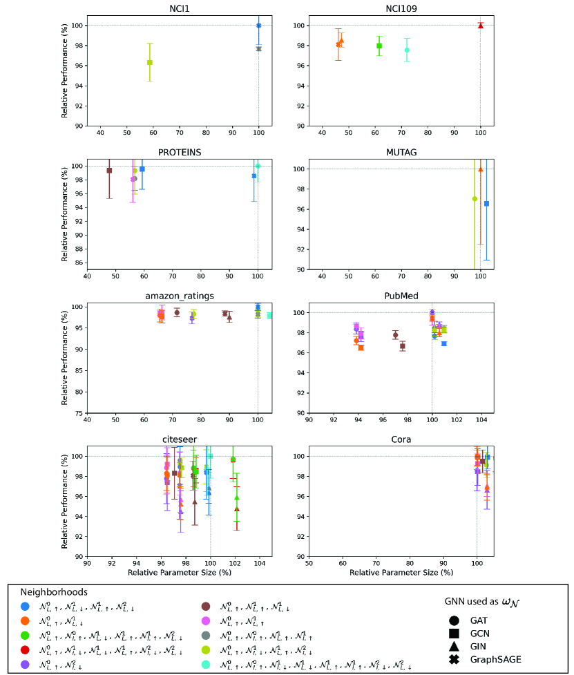
Figure 6: Performance versus Size, scaled to best-performing model.

References

- Agarwal et al. (2006) Sameer Agarwal, Kristin Branson, and Serge Belongie. Higher order learning with graphs. In Proceedings of the 23rd international conference on Machine learning, pp. 17–24, 2006.
- Antelmi et al. (2023) Alessia Antelmi, Gennaro Cordasco, Mirko Polato, Vittorio Scarano, Carmine Spagnuolo, and Dingqi Yang. A survey on hypergraph representation learning. ACM Comput. Surv., 56(1), aug 2023. ISSN 0360-0300. doi: 10.1145/3605776. URL https://doi.org/10.1145/3605776.
- Bandyopadhyay et al. (2020) Sambaran Bandyopadhyay, Kishalay Das, and M Narasimha Murty. Line hypergraph convolution network: Applying graph convolution for hypergraphs. arXiv preprint arXiv:2002.03392, 2020.
- Battiloro et al. (2023) Claudio Battiloro, Lucia Testa, Lorenzo Giusti, Stefania Sardellitti, Paolo Di Lorenzo, and Sergio Barbarossa. Generalized simplicial attention neural networks. arXiv preprint arXiv:2309.02138, 2023.
- Battiloro et al. (2024) Claudio Battiloro, Ege Karaismailoğlu, Mauricio Tec, George Dasoulas, Michelle Audirac, and Francesca Dominici. E (n) equivariant topological neural networks. arXiv preprint arXiv:2405.15429, 2024.
- Bodnar (2023) Cristian Bodnar. Topological Deep Learning: Graphs, Complexes, Sheaves. PhD thesis, Cambridge University, 2023.
- Bodnar et al. (2021a) Cristian Bodnar, Fabrizio Frasca, Nina Otter, Yuguang Wang, Pietro Lio, Guido F Montufar, and Michael Bronstein. Weisfeiler and Lehman Go Cellular: CW Networks. Advances in Neural Information Processing Systems, 34:2625–2640, 2021a.
- Bodnar et al. (2021b) Cristian Bodnar, Fabrizio Frasca, Yuguang Wang, Nina Otter, Guido F Montufar, Pietro Lio, and Michael Bronstein. Weisfeiler and Lehman Go Topological: Message Passing Simplicial Networks. In International Conference on Machine Learning, pp. 1026–1037. PMLR, 2021b.
- Bolla (1993) Marianna Bolla. Spectra, euclidean representations and clusterings of hypergraphs. Discrete Mathematics, 117(1-3):19–39, 1993.
- Chen et al. (2020a) Chaofan Chen, Zelei Cheng, Zuotian Li, and Manyi Wang. Hypergraph attention networks. In 2020 IEEE 19th International Conference on Trust, Security and Privacy in Computing and Communications (TrustCom), pp. 1560–1565. IEEE, 2020a.
- Chen et al. (2020b) Yu Chen, Lingfei Wu, and Mohammed Zaki. Iterative deep graph learning for graph neural networks: Better and robust node embeddings. In H. Larochelle, M. Ranzato, R. Hadsell, M.F. Balcan, and H. Lin (eds.), Advances in Neural Information Processing Systems, volume 33, pp. 19314–19326. Curran Associates, Inc., 2020b. URL https://proceedings.neurips.cc/paper/2020/file/e05c7ba4e087beea9410929698dc41a6-Paper.pdf.
- Corso et al. (2024) Gabriele Corso, Hannes Stark, Stefanie Jegelka, Tommi Jaakkola, and Regina Barzilay. Graph neural networks. Nature Reviews Methods Primers, 4(1):17, 2024.
- Ebli et al. (2020) S. Ebli, M. Defferrard, and G. Spreemann. Simplicial neural networks. In Advances in Neural Information Processing Systems Workshop on Topological Data Analysis and Beyond, 2020.
- Eitan et al. (2024) Yam Eitan, Yoav Gelberg, Guy Bar-Shalom, Fabrizio Frasca, Michael Bronstein, and Haggai Maron. Topological blind spots: Understanding and extending topological deep learning through the lens of expressivity. arXiv preprint arXiv:2408.05486, 2024.
- Feng et al. (2019) Yifan Feng, Haoxuan You, Zizhao Zhang, Rongrong Ji, and Yue Gao. Hypergraph neural networks. In Proceedings of the AAAI conference on artificial intelligence, volume 33, pp. 3558–3565, 2019.
- Fey & Lenssen (2019) M. Fey and J. E. Lenssen. Fast graph representation learning with PyTorch Geometric. In International Conference on Learning Representations Workshop on Representation Learning on Graphs and Manifolds, 2019.
- Gibson et al. (2000) David Gibson, Jon Kleinberg, and Prabhakar Raghavan. Clustering categorical data: An approach based on dynamical systems. The VLDB Journal, 8:222–236, 2000.
- Gilmer et al. (2017) Justin Gilmer, Samuel S. Schoenholz, Patrick F. Riley, Oriol Vinyals, and George E. Dahl. Neural message passing for quantum chemistry. In Proceedings of the 34th International Conference on Machine Learning - Volume 70, ICML’17, pp. 1263–1272. JMLR.org, 2017.
- Giusti et al. (2022a) Lorenzo Giusti, Claudio Battiloro, Paolo Di Lorenzo, Stefania Sardellitti, and Sergio Barbarossa. Simplicial attention networks. arXiv preprint arXiv:2203.07485, 2022a.
- Giusti et al. (2022b) Lorenzo Giusti, Claudio Battiloro, Lucia Testa, Paolo Di Lorenzo, Stefania Sardellitti, and Sergio Barbarossa. Cell attention networks. arXiv preprint arXiv:2209.08179, 2022b.
- Hajij et al. (2020) Mustafa Hajij, Kyle Istvan, and Ghada Zamzmi. Cell complex neural networks. In Advances in Neural Information Processing Systems Workshop on TDA & Beyond, 2020.
- Hajij et al. (2023) Mustafa Hajij, Ghada Zamzmi, Theodore Papamarkou, Nina Miolane, Aldo Guzmán-Sáenz, Karthikeyan Natesan Ramamurthy, Tolga Birdal, Tamal Dey, Soham Mukherjee, Shreyas Samaga, Neal Livesay, Robin Walters, Paul Rosen, and Michael Schaub. Topological deep learning: Going beyond graph data. arXiv preprint arXiv:1906.09068 (v3), 2023.
- Hajij et al. (2024a) Mustafa Hajij, Theodore Papamarkou, Ghada Zamzmi, Karthikeyan Natesan Ramamurthy, Tolga Birdal, and Michael T. Schaub. Topological Deep Learning: Going Beyond Graph Data. Online, 2024a. URL http://tdlbook.org. Published online on August 6, 2024.
- Hajij et al. (2024b) Mustafa Hajij, Mathilde Papillon, Florian Frantzen, Jens Agerberg, Ibrahem AlJabea, Ruben Ballester, Claudio Battiloro, Guillermo Bernárdez, Tolga Birdal, Aiden Brent, et al. Topox: a suite of python packages for machine learning on topological domains. arXiv preprint arXiv:2402.02441, 2024b.
- Hamilton et al. (2017) William L. Hamilton, Rex Ying, and Jure Leskovec. Inductive representation learning on large graphs. In Proceedings of the 31st International Conference on Neural Information Processing Systems, NIPS’17, pp. 1025–1035, Red Hook, NY, USA, 2017. Curran Associates Inc. ISBN 9781510860964.
- Irwin et al. (2012) John J Irwin, Teague Sterling, Michael M Mysinger, Erin S Bolstad, and Ryan G Coleman. ZINC: a free tool to discover chemistry for biology. Journal of Chemical Information and Modeling, 52(7):1757–1768, 2012.
- Jogl et al. (2022a) Fabian Jogl, Maximilian Thiessen, and Thomas Gärtner. Reducing learning on cell complexes to graphs. In ICLR 2022 Workshop on Geometrical and Topological Representation Learning, 2022a.
- Jogl et al. (2022b) Fabian Jogl, Maximilian Thiessen, and Thomas Gärtner. Weisfeiler and leman return with graph transformations. In 18th International Workshop on Mining and Learning with Graphs, 2022b.
- Jogl et al. (2023) Fabian Jogl, Maximilian Thiessen, and Thomas Gärtner. Expressivity-preserving GNN simulation. In Thirty-seventh Conference on Neural Information Processing Systems, 2023. URL https://openreview.net/forum?id=ytTfonl9Wd.
- Jogl et al. (2024) Fabian Jogl, Maximilian Thiessen, and Thomas Gärtner. Expressivity-preserving gnn simulation. Advances in Neural Information Processing Systems, 36, 2024.
- Kipf & Welling (2017) Thomas N. Kipf and Max Welling. Semi-supervised classification with graph convolutional networks. In International Conference on Learning Representations (ICLR), 2017.
- Lambiotte et al. (2019) R. Lambiotte, M. Rosvall, and I. Scholtes. From networks to optimal higher-order models of complex systems. Nature physics, 2019.
- Maggs et al. (2024) Kelly Maggs, Celia Hacker, and Bastian Rieck. Simplicial representation learning with neural $k$-forms. In The Twelfth International Conference on Learning Representations, 2024. URL https://openreview.net/forum?id=Djw0XhjHZb.
- Morris et al. (2020) C. Morris, N. M. Kriege, F. Bause, K. Kersting, P. Mutzel, and M. Neumann. Tudataset: A collection of benchmark datasets for learning with graphs. arXiv preprint arXiv:2007.08663, 2020.
- Papamarkou et al. (2024) Theodore Papamarkou, Tolga Birdal, Michael Bronstein, Gunnar Carlsson, Justin Curry, Yue Gao, Mustafa Hajij, Roland Kwitt, Pietro Liò, Paolo Di Lorenzo, et al. Position paper: Challenges and opportunities in topological deep learning. arXiv preprint arXiv:2402.08871, 2024.
- Papillon et al. (2023) Mathilde Papillon, Sophia Sanborn, Mustafa Hajij, and Nina Miolane. Architectures of topological deep learning: A survey on topological neural networks, 2023.
- Paszke et al. (2019) A. Paszke, S. Gross, F. Massa, A. Lerer, J. Bradbury, G. Chanan, T. Killeen, Z. Lin, N. Gimelshein, L. Antiga, A. Desmaison, A. Kopf, E. Yang, Z. DeVito, M. Raison, A. Tejani, S. Chilamkurthy, B. Steiner, L. Fang, J. Bai, and S. Chintala. Pytorch: An imperative style, high-performance deep learning library. In Advances in Neural Information Processing Systems. 2019.
- Roddenberry et al. (2021) T Mitchell Roddenberry, Nicholas Glaze, and Santiago Segarra. Principled simplicial neural networks for trajectory prediction. In International Conference on Machine Learning, pp. 9020–9029. PMLR, 2021.
- Rodríguez (2002) Juan A Rodríguez. On the laplacian eigenvalues and metric parameters of hypergraphs. Linear and Multilinear Algebra, 50(1):1–14, 2002.
- Scarselli et al. (2008) F. Scarselli, M. Gori, A. C. Tsoi, M. Hagenbuchner, and G. Monfardini. The graph neural network model. IEEE Transactions on Neural Networks, 2008.
- Solé et al. (1996) Patrick Solé et al. Spectra of regular graphs and hypergraphs and orthogonal polynomials. European Journal of Combinatorics, 17(5):461–477, 1996.
- Telyatnikov et al. (2023) Lev Telyatnikov, Maria Sofia Bucarelli, Guillermo Bernardez, Olga Zaghen, Simone Scardapane, and Pietro Lio. Hypergraph neural networks through the lens of message passing: a common perspective to homophily and architecture design. arXiv preprint arXiv:2310.07684, 2023.
- Telyatnikov et al. (2024) Lev Telyatnikov, Guillermo Bernardez, Marco Montagna, Pavlo Vasylenko, Ghada Zamzmi, Mustafa Hajij, Michael T Schaub, Nina Miolane, Simone Scardapane, and Theodore Papamarkou. Topobenchmarkx: A framework for benchmarking topological deep learning. arXiv preprint arXiv:2406.06642, 2024.
- Vaswani et al. (2017) A. Vaswani, N. Shazeer, N. Parmar, J. Uszkoreit, L. Jones, A. N. Gomez, L. Kaiser, and I. Polosukhin. Attention is all you need. In Advances in Neural Information Processing Systems, 2017.
- Veličković (2022) Petar Veličković. Message passing all the way up. arXiv preprint arXiv:2202.11097, 2022.
- Velickovic et al. (2017) Petar Velickovic, Guillem Cucurull, Arantxa Casanova, Adriana Romero, Pietro Lio, Yoshua Bengio, et al. Graph attention networks. stat, 1050(20):10–48550, 2017.
- Xu et al. (2019a) K. Xu, W. Hu, J. Leskovec, and S. Jegelka. How powerful are graph neural networks? In International Conference on Learning Representations, 2019a.
- Xu et al. (2019b) Keyulu Xu, Weihua Hu, Jure Leskovec, and Stefanie Jegelka. How powerful are graph neural networks? In International Conference on Learning Representations, 2019b. URL https://openreview.net/forum?id=ryGs6iA5Km.
- Yadati (2020) Naganand Yadati. Neural message passing for multi-relational ordered and recursive hypergraphs. Advances in Neural Information Processing Systems, 33:3275–3289, 2020.
- Yang & Isufi (2023) Maosheng Yang and Elvin Isufi. Convolutional learning on simplicial complexes. arXiv preprint arXiv:2301.11163, 2023.
- Yang et al. (2022) Ruochen Yang, Frederic Sala, and Paul Bogdan. Efficient representation learning for higher-order data with simplicial complexes. In Bastian Rieck and Razvan Pascanu (eds.), Proceedings of the First Learning on Graphs Conference, volume 198 of Proceedings of Machine Learning Research, pp. 13:1–13:21. PMLR, 09–12 Dec 2022. URL https://proceedings.mlr.press/v198/yang22a.html.
- Yang et al. (2016) Zhilin Yang, William Cohen, and Ruslan Salakhudinov. Revisiting semi-supervised learning with graph embeddings. In International conference on machine learning, pp. 40–48. PMLR, 2016.
- Zhang & Chen (2018) M. Zhang and Y. Chen. Link prediction based on graph neural networks. Advances in Neural Information Processing Systems, 2018.
- Zhou et al. (2006) Dengyong Zhou, Jiayuan Huang, and Bernhard Schölkopf. Learning with hypergraphs: Clustering, classification, and embedding. Advances in neural information processing systems, 19, 2006.