Quasi-stationary Subdivision Schemes in Arbitrary Dimensions

Abstract.

Stationary subdivision schemes have been extensively studied and have numerous applications in CAGD and wavelet analysis. To have high-order smoothness of the scheme, it is usually inevitable to enlarge the support of the mask that is used, which is a major difficulty with stationary subdivision schemes due to complicated implementation and dramatically increased special subdivision rules at extraordinary vertices. In this paper, we introduce the notion of a multivariate quasi-stationary subdivision scheme and fully characterize its convergence and smoothness. We will also discuss the general procedure of designing interpolatory masks with short support that yields smooth quasi-stationary subdivision schemes. Specifically, using the dyadic dilation of both triangular and quadrilateral meshes, for each smoothness exponent $m=1,2$, we obtain examples of $C^{m}$-convergent quasi-stationary $2I_{2}$-subdivision schemes with bivariate symmetric masks having at most $m$-ring stencils. Our examples demonstrate the advantage of quasi-stationary subdivision schemes, which can circumvent the difficulty above with stationary subdivision schemes.

1. Introduction and Motivation

Subdivision schemes are fast iterative averaging algorithms for computing refinable functions and wavelets. Due to the cascade/multi-scale structure and intrinsic connections to splines and wavelets, subdivision schemes are of great interest in many applications such as computer-aided geometric design (CAGD) for generating smooth curves and surfaces ([8, 11, 12, 13, 14, 23, 25, 28, 34]), solving PDEs numerically using multi-scale methods ([27] and references therein), and data processing with discrete wavelet/framelet transforms ([20, 26]). This paper focuses on multivariate quasi-stationary subdivision schemes in arbitrary dimensions. In this section, we recall some basics of subdivision schemes and explain the motivations and contributions of our work.

1.1. Stationary subdivision schemes: convergence and smoothness

The classical way to implement a subdivision scheme is by performing a subdivision operation using the same mask at every level, and such a scheme is often known as a stationary subdivision scheme. To be specific, let us introduce some basic notations. By a $d$-dimensional mask/filter we mean a sequence $a=\{a(k)\}_{k\in\mathbb{Z}^{d}}:\mathbb{Z}^{d}\to\mathbb{C}$ such that $a(k)\neq 0$ for only finitely many terms. By $l_{0}(\mathbb{Z}^{d})$ we denote the linear space of all $d$-dimensional filters. To perform a subdivision scheme, we need a mask $a\in l_{0}(\mathbb{Z}^{d})$ normalized by

$$\sum_{k\in\mathbb{Z}^{d}}a(k)=1,$$ (1.1)

and we shall use a dilation matrix $\mathsf{M}I_{d}$ where $\mathsf{M}\in\mathbb{N}\setminus\{1\}$ and $I_{d}$ denotes the $d\times d$ identity matrix. The $\mathsf{M}I_{d}$-subdivision operator $\mathcal{S}_{a,\mathsf{M}I_{d}}$ that uses the mask $a$ is then defined by

$$[\mathcal{S}_{a,\mathsf{M}I_{d}}v](k):=\mathsf{M}^{d}\sum_{n\in\mathbb{Z}^{d}}v(n)a(k-\mathsf{M}n),\quad\forall v\in l_{0}(\mathbb{Z}^{d}),\,k\in\mathbb{Z}^{d}.$$

Given an initial data $v\in l_{0}(\mathbb{Z}^{d})$, the stationary $\mathsf{M}I_{d}$-subdivision scheme that employs the mask $a$ iteratively generates a sequence $\{\mathcal{S}_{a,\mathsf{M}I_{d}}^{n}v\}_{n=1}^{\infty}$, which is expected to converge, after locating the value $[\mathcal{S}_{a,\mathsf{M}I_{d}}^{n}v](k)$ at the position $\mathsf{M}^{-n}k$ for $k\in\mathbb{Z}^{d}$, to a smooth function/surface $\eta_{v}$.

Stationary subdivision schemes are closely related to refinable functions. For a mask $a\in l_{0}(\mathbb{Z}^{d})$ satisfying (1.1) and for a dilation matrix $\mathsf{M}I_{d}$, it is well known that there exists a compactly supported distribution $\phi$ such that the following $\mathsf{M}I_{d}$-refinement equation holds:

$$\phi(x)=\mathsf{M}^{d}\sum_{k\in\mathbb{Z}^{d}}a(k)\phi(\mathsf{M}x-k),\qquad\forall x\in\mathbb{R}^{d}.$$ (1.2)

Any $\phi$ satisfying (1.2) is called an $\mathsf{M}I_{d}$-refinable function of the mask $a$. In such cases, the mask $a$ is called the $\mathsf{M}I_{d}$-refinement mask of the distribution $\phi$. One powerful tool for studying refinable properties is the Fourier transform. For $f\in L_{1}(\mathbb{R}^{d})$, its Fourier transform is defined by

$$\widehat{f}(\xi):=\int_{\mathbb{R}^{d}}f(x)e^{-ix\cdot\xi}dx,\qquad\forall\xi\in\mathbb{R}^{d}.$$

The definition of the Fourier transform is naturally extended to tempered distributions. For any $a\in l_{0}(\mathbb{Z}^{d})$, define its Fourier series by

$$\widehat{a}(\xi):=\sum_{k\in\mathbb{Z}^{d}}a(k)e^{-ik\cdot\xi},\qquad\forall\xi\in\mathbb{R}^{d}.$$

Using the Fourier transform, (1.2) is equivalent to

$$\widehat{\phi}(\mathsf{M}\xi)=\widehat{a}(\xi)\widehat{\phi}(\xi),\qquad\forall\xi\in\mathbb{R}^{d}.$$ (1.3)

Suppose $a\in l_{0}(\mathbb{Z}^{d})$ satisfies $\widehat{a}(0)=1$ (this condition is equivalent to $\sum_{k\in\mathbb{Z}^{d}}a(k)=1$ in (1.1)), one can define a compactly supported distribution $\phi$ through its Fourier transform by

$$\widehat{\phi}(\xi):=\prod_{j=1}^{\infty}\widehat{a}(\mathsf{M}^{-j}\xi),\qquad\forall\xi\in\mathbb{R}^{d}.$$ (1.4)

Then clearly $\phi$ satisfies (1.2) with $\widehat{\phi}(0)=1$. In this case, the above function $\phi$ is called the standard $\mathsf{M}I_{d}$-refinable function of the mask $a$. Generally, an $\mathsf{M}I_{d}$-refinable function $\phi$ of a mask $a\in l_{0}(\mathbb{Z}^{d})$ does not have an analytic explicit expression. Fortunately, one can approximate $\phi$ by implementing the $\mathsf{M}I_{d}$-subdivision scheme with its refinement mask $a$, provided that the scheme is convergent. Let $a\in l_{0}(\mathbb{Z}^{d})$ be such that $\widehat{a}(0)=1$ and $\mathsf{M}\in\mathbb{N}\setminus\{1\}$. If for every $v\in l_{0}(\mathbb{Z}^{d})$, there exists a continuous $d$-dimensional function $\eta_{v}$ on $\mathbb{R}^{d}$ such that

$$\lim_{n\to\infty}\sup_{k\in\mathbb{Z}^{d}}|[\mathcal{S}_{a,\mathsf{M}I_{d}}^{n}v](k)-\eta_{v}(\mathsf{M}^{-n}k)|=0,$$

then we say that the $\mathsf{M}I_{d}$-subdivision scheme with the $d$-dimensional mask $a$ is convergent. It is known (e.g., see [18, Theorem 4.3] or [20, Theorem 7.3.1]) that the $\mathsf{M}I_{d}$-subdivision scheme with a mask $a\in l_{0}(\mathbb{Z}^{d})$ is convergent if and only if $\operatorname{sm}_{\infty}(a,\mathsf{M}I_{d})>0$ (see (1.12) for its definition). For a convergent $\mathsf{M}I_{d}$-subdivision scheme employing a mask $a\in l_{0}(\mathbb{Z}^{d})$, if $v(k)=\boldsymbol{\delta}(k)$ for all $k\in\mathbb{Z}^{d}$, where

$$\boldsymbol{\delta}(x):=\begin{cases}1,&x=0,\\ 0,&x\in\mathbb{R}^{d}\setminus\{0\},\end{cases}$$ (1.5)

then the limit function $\eta_{\boldsymbol{\delta}}$ is the standard $\mathsf{M}I_{d}$-refinable function $\phi$ that is defined via (1.4).

For a convergent subdivision scheme, if any initial data $v\in l_{0}(\mathbb{Z}^{d})$ can be interpolated by its limit function $\eta_{v}$, that is,

$$\eta_{v}(k)=v(k),\qquad\forall k\in\mathbb{Z}^{d},$$

then the subdivision scheme is $\mathsf{M}I_{d}$-interpolatory. Interpolatory subdivision schemes are important in sampling theory, signal processing, and CAGD. The literature has extensively studied their theoretical properties and applications (e.g., see [12, 13, 4, 5, 10, 21, 24, 25, 31, 32, 15] and many references therein). For a convergent $\mathsf{M}I_{d}$-subdivision scheme that employs the mask $a\in l_{0}(\mathbb{Z}^{d})$, using the linearity of the subdivision operator, the limit function $\eta_{v}$ of any input data $v\in l_{0}(\mathbb{Z}^{d})$ must satisfy

$$\eta_{v}(x)=\sum_{k\in\mathbb{Z}^{d}}v(k)\phi(x-k),\qquad\forall x\in\mathbb{R}^{d},$$

where $\phi$ is the standard $\mathsf{M}I_{d}$-refinable function associated with the mask $a$ that is defined via (1.4). Therefore, a convergent $\mathsf{M}I_{d}$-subdivision scheme is $\mathsf{M}I_{d}$-interpolatory if and only if the $\mathsf{M}I_{d}$-refinable function $\phi$ is interpolatory, that is, $\phi$ is continuous and

$$\phi(k)=\boldsymbol{\delta}(k),\quad\forall k\in\mathbb{Z}^{d}.$$ (1.6)

Furthermore, for a convergent subdivision scheme, (1.6) implies

$$a(\mathsf{M}k)=\mathsf{M}^{-d}\boldsymbol{\delta}(k),\quad\forall k\in\mathbb{Z}^{d},$$ (1.7)

that is, $a$ must be an $\mathsf{M}I_{d}$-interpolatory mask. For an $\mathsf{M}I_{d}$-refinable function $\phi$ with a finitely supported mask $a\in l_{0}(\mathbb{Z}^{d})$, it is known (e.g., see [18, Corollary 5.2]) that $\phi$ is interpolating if and only if $\operatorname{sm}_{\infty}(a,\mathsf{M}I_{d})>0$ and the mask $a$ is $\mathsf{M}I_{d}$-interpolatory.

In applications such as CAGD, to have good visual quality of the generated subdivision curves or surfaces, a stationary subdivision scheme of high-order smoothness is desired. Smooth stationary subdivision schemes and their applications have been well-studied in the literature; see, for instance, [1, 6, 11, 20, 23, 25] and many references therein. To define the smoothness of a stationary subdivision scheme, for $h\in\mathbb{Z}^{d}$, we first define the backward difference operator $\nabla_{h}$ by:

$$\nabla_{h}v(k)=v(k)-v(k-h),\quad\forall v\in l_{0}(\mathbb{Z}^{d}),\,k\in\mathbb{Z}^{d}.$$

For every $\mu=(\mu_{1},\dots,\mu_{d})\in\mathbb{N}_{0}^{d}$, we define

$$\nabla^{\mu}:=\nabla^{\mu_{1}}_{e_{1}}\dots\nabla^{\mu_{d}}_{e_{d}},$$

where $e_{j}$ is the $j$-th coordinate vector in $\mathbb{R}^{d}$ for all $j=1,\dots,d$. For any $\mu\in\mathbb{N}_{0}^{d}$ and $v\in l_{0}(\mathbb{Z}^{d})$, observe that $\nabla^{\mu}v=[\nabla^{\mu}\boldsymbol{\delta}]*v$, where the convolution of two filters $v,u\in l_{0}(\mathbb{Z}^{d})$ is defined as

$$[v*u](k):=\sum_{q\in\mathbb{Z}^{d}}v(k-q)u(q),\qquad\forall k\in\mathbb{Z}^{d}.$$

It is straightforward to check that

$$\widehat{\nabla^{\mu}v}(\xi)=\widehat{\nabla^{\mu}\boldsymbol{\delta}}(\xi)\widehat{v}(\xi)=(1-e^{-i\xi_{1}})^{\mu_{1}}\dots(1-e^{-i\xi_{d}})^{\mu_{d}}\widehat{v}(\xi),\quad\forall\xi=(\xi_{1},\dots,\xi_{d})\in\mathbb{R}^{d}.$$

Next, we recall the notion of $C^{m}$-convergence where $m\in\mathbb{N}_{0}$ measures the order of smoothness. Let $s\in\mathbb{N}_{0}$ and $a\in l_{0}(\mathbb{Z}^{d})$ satisfying $\widehat{a}(0)=1$. If for every initial data $v\in l_{0}(\mathbb{Z}^{d})$, there exists $\eta_{v}\in C^{m}(\mathbb{R}^{d})$ such that

$$\lim_{n\to\infty}\sup_{k\in\mathbb{Z}^{d}}\left|\mathsf{M}^{jn}[\nabla^{\mu}\mathcal{S}_{a,\mathsf{M}I_{d}}^{n}v](k)-\partial^{\mu}\eta_{v}(\mathsf{M}^{-n}k)\right|=0,\quad\forall\mu\in\mathbb{N}_{0,j}^{d},\,j=0,1,\dots,m,$$ (1.8)

where $\mathbb{N}_{0,j}^{d}:=\{\mu\in\mathbb{N}_{0}^{d}:|\mu|=j\},$ then we say that the $\mathsf{M}I_{d}$-subdivision scheme that employs the mask $a$ is $C^{m}$-convergent. The smoothness of a stationary subdivision scheme is fully characterized by its underlying mask $a$. To do this, we need to introduce two technical quantities: the sum rule orders and the smoothness exponenets of the mask $a$. Let $f$ and $g$ be smooth functions and $m\in\mathbb{N}_{0}$, recall the following big $\mathscr{O}$ notation:

$$f(\xi)=g(\xi)+\mathscr{O}(\|\xi-\xi_{0}\|^{m}),\quad\xi\to\xi_{0},$$

which means

$$\partial^{\mu}f(\xi_{0})=\partial^{\mu}g(\xi_{0}),\quad\forall\mu\in\mathbb{N}_{0}^{d}\text{ such that }|\mu|<m.$$

Let $a\in l_{0}(\mathbb{Z}^{d})$ be a $d$-dimensional filter and $\mathsf{M}\in\mathbb{N}\setminus\{1\}$.

1. For $m\in\mathbb{N}_{0}$, we say that the mask $a$ has order $m$ sum rules with respect to $\mathsf{M}I_{d}$ if

   $$\sum_{k\in\mathbb{Z}^{d}}(\gamma+\mathsf{M}k)^{\mu}a(\gamma+\mathsf{M}k)=\mathsf{M}^{-d}\sum_{k\in\mathbb{Z}^{d}}k^{\mu}a(k),\quad\forall\gamma\in\mathbb{Z}^{d},\,\mu\in\mathbb{N}_{0}^{d}\text{ such that }|\mu|<m,$$ (1.9)

   or equivalently,

   $$\widehat{a}(\xi+2\pi\omega)=\mathscr{O}(\|\xi\|^{m}),\quad\xi\to 0,\qquad\forall\omega\in\Omega_{\mathsf{M}}\setminus\{0\},$$ (1.10)

   where

   $$\Omega_{\mathsf{M}}:=[\mathsf{M}^{-1}\mathbb{Z}^{d}]\cap[0,1)^{d}.$$ (1.11)

   Define

   $$\operatorname{sr}(a,\mathsf{M}I_{d}):=\sup\{m\in\mathbb{N}_{0}:\,\text{\eqref{sr:def} or \eqref{sr} holds}\}.$$

2. Let $1\leqslant p\leqslant\infty$ and suppose $\operatorname{sr}(a,\mathsf{M}I_{d})=m$. We define

   $$\rho_{m}(a,\mathsf{M}I_{d})_{p}:=\sup\left\{\limsup_{n\to\infty}\left\|\nabla^{\mu}\mathcal{S}_{a,\mathsf{M}}^{n}\boldsymbol{\delta}\right\|_{l_{p}(\mathbb{Z}^{d})}^{1/n}:\,\mu\in\mathbb{N}_{0,m}^{d}\right\},$$

   and the $L_{p}$-smoothness exponent of the mask $a$ (with respect to $\mathsf{M}I_{d}$) by

   $$\operatorname{sm}_{p}(a,\mathsf{M}I_{d}):=\frac{d}{p}-\log_{\mathsf{M}}[\rho_{m}(a,\mathsf{M}I_{d})_{p}].$$ (1.12)

By [18, Theorem 4.3] (also see [25, Theorem 2.1] and [20, Theorem 7.3.1]), the stationary $\mathsf{M}I_{d}$-subdivision scheme that employs the mask $a$ is $C^{m}$-convergent if and only if $\operatorname{sm}_{\infty}(a,\mathsf{M}I_{d})>m$. In particular, for a $C^{m}$-convergent stationary subdivision scheme, the standard $\mathsf{M}I_{d}$-refinable function $\phi$ derived from the mask $a$ via (1.4) belongs to $C^{m}(\mathbb{R}^{d})$. Furthermore,the partial derivative $\partial^{\mu}\phi$ is compactly supported and uniformly continuous for all $\mu\in\mathbb{N}_{0}^{d}$ with $|\mu|\leqslant m$. Generally, there is no efficient way to compute $\operatorname{sm}_{\infty}(a,\mathsf{M}I_{d})$. One way to estimate $\operatorname{sm}_{\infty}(a,\mathsf{M}I_{d})$ is from $\operatorname{sm}_{2}(a,\mathsf{M}I_{d})$ which can be efficiently computed (e.g. see [18, 19, 30]). Using the definition of the $L_{p}$-smoothness exponent, one can directly obtain the following lower bound of $\operatorname{sm}_{\infty}(a,\mathsf{M}I_{d})$ (e.g., see [19, Theorem 3.1] or [33, Lemma 3.1]):

$$\operatorname{sm}_{\infty}(a,\mathsf{M}I_{d})\geqslant\operatorname{sm}_{2}(a,\mathsf{M}I_{d})-\frac{d}{2}.$$ (1.13)

If the mask $a$ has a specific form, then we may be able to get a more accurate estimation of $\operatorname{sm}_{\infty}(a,\mathsf{M}I_{d})$. See Section 3 for estimations of $\operatorname{sm}_{\infty}(a,4I_{2})$ for specific two-dimensional masks $a$ in our examples.

1.2. Motivation from CAGD and difficulties with stationary subdivision schemes

In applications, we often require the underlying mask $a$ to satisfy certain critical properties for different purposes. First, one prefers a subdivision scheme that employs a mask with short support for the efficiency of implementation and computation. In the settings of CAGD, this is described by the size of stencils of a mask (or a scheme). To be specific, for a mask $a\in l_{0}(\mathbb{Z}^{d})$, we define its filter support to be the smallest $d$-dimensional interval $I:=[k_{1,1},k_{1,2}]\times[k_{2,1},k_{2,2}]\times\dots\times[k_{d,1},k_{d,2}]$ where $k_{1,1},k_{1,2},\dots,k_{d,1},k_{d,2}\in\mathbb{Z}$ such that $a(k)=0$ whenever $k\notin I$. A stationary $\mathsf{M}I_{d}$-subdivision scheme with a mask $a\in l_{0}(\mathbb{Z}^{d})$ has $n$-ring stencils for some $n\in\mathbb{N}$ if $\text{fsupp}(a)\subseteq[-\mathsf{M}n,\mathsf{M}n]^{d}$. In general, it is highly desirable to have a $n$-ring stencil subdivision scheme such that $n$ is as small as possible, and that is, the mask $a$ has very small support. Next, a curve or a surface is modeled by a mesh by connecting neighborhood points. For example, in dimension two, there are two standard meshes: the triangular mesh and the quadrilateral mesh. A particular mesh is often associated with a symmetry group, and thus, the underlying mask of a subdivision scheme is often required to have the corresponding symmetry type.

In applications such as CAGD, people are particularly interested in a subdivision scheme that: (1) is interpolatory so that the limit function interpolates the initial data; (2) is at least $C^{2}$-convergent for the continuity of curvatures; (3) has no more than $2$-ring stencils to avoid exponentially increasing number of special subdivision rules near extraordinary vertices; (4) employs a mask with symmetry for a particular mesh. Unfortunately, these good properties cannot coexist in many cases. Suppose $a\in l_{0}(\mathbb{Z}^{d})$ is $\mathsf{M}I_{d}$-interpolatory ($\mathsf{M}\in\mathbb{N}\setminus\{1\}$), supported on $[-\mathsf{M},\mathsf{M}]^{d}$ ( that is, has $1$-ring stencil) and satisfies $a(k)=a(-k)$ for all $k\in\mathbb{Z}^{d}$ (this is the weakest symmetry type). On one hand, by [25, Theorem 3.4] (also see [17, Theorem 4.1]), we have $\operatorname{sr}(a,2I_{d})\leqslant 2$ and therefore $\operatorname{sm}_{\infty}(a,\mathsf{M}I_{2})\leqslant 2$. It then follows from [16, Theorem 3.8] that the standard $\mathsf{M}I_{d}$-refinable function $\phi$ of the mask $a$ is not a $C^{2}(\mathbb{R}^{d})$ function, so the stationary subdivision scheme that uses the mask $a$ cannot be $C^{2}$-convergent. Hence, any $C^{2}$-convergent interpolatory stationary $\mathsf{M}I_{d}$-subdivision scheme that uses a symmetric mask must have at least $2$-ring stencils. On the other hand, for the most classical dilation matrix $2I_{d}$, it is pointed out in [17, Corollary 4.3 and Theorem 3.5] and [16, Theorem 3.9 and Corollary 3.12] that a $C^{2}$-convergent interpolatory stationary $2I_{d}$-subdivision scheme must have at least $3$-ring stencils. Consequently, the mutual conflict between properties (1)-(4) is a major difficulty with stationary subdivision schemes. Indeed, many existing famous stationary subdivision schemes do not satisfy all these properties. For instance, the famous butterfly scheme in [13] (also see [7] for a non-linear analog of the scheme) and the interpolatory $2I_{d}$-subdivision schemes in [23, 39] all have no more than $2$-ring stencils but are not $C^{2}$-convergent; other modified butterfly schemes achieve $C^{2}$-convergence by either enlarging the support of the mask ([36]) or making the mask to have $2$-ring stencils but sacrificing the interpolatory property ([29]). Therefore, we need new settings and ideas to circumvent this difficulty with stationary subdivision schemes.

1.3. Our contribution and paper structure

To resolve the potential conflict between high-order smoothness and the short support of a refinement mask, following [22], we introduce the notion of a quasi-stationary subdivision scheme. Unlike a stationary subdivision scheme, a quasi-stationary subdivision scheme employs several different refinement masks repeatedly at different levels. Let $\mathsf{M}\in\mathbb{N}\setminus\{1\}$ be a dilation factor. For $r\in\mathbb{N}$ and $a_{1},\dots,a_{r}\in l_{0}(\mathbb{Z}^{d})$, define

$$\mathcal{S}_{a_{1},\dots,a_{r},\mathsf{M}I_{d}}^{n,r}:=\begin{cases}[\mathcal{S}_{a_{r},\mathsf{M}I_{d}}\dots\mathcal{S}_{a_{1},\mathsf{M}I_{d}}]^{\lfloor\frac{n}{r}\rfloor},&\text{if }n\in r\mathbb{N}_{0},\\ \mathcal{S}_{a_{l},\mathsf{M}I_{d}}\dots\mathcal{S}_{a_{1},\mathsf{M}I_{d}}[\mathcal{S}_{a_{r},\mathsf{M}I_{d}}\dots\mathcal{S}_{a_{1},\mathsf{M}}]^{\lfloor\frac{n}{r}\rfloor},&\text{if }n\in r\mathbb{N}_{0}+l\text{ for some }l\in\{1,\dots,r-1\}.\end{cases}$$

Suppose $\widehat{a_{l}}(0)=1$ for all $l=1,\dots,r$. Given an initial data $v\in l_{0}(\mathbb{Z}^{d})$, the $r$-mask quasi-stationary $\mathsf{M}I_{d}$-subdivision scheme that uses $a_{1},\dots,a_{r}$ generates a sequence $\{\mathcal{S}_{a_{1},\dots,a_{r},\mathsf{M}I_{d}}^{n,r}v\}_{n=1}^{\infty}$. When $r=1$, an $r$-mask quasi-stationary subdivision scheme becomes a stationary one. We define the $C^{m}$-convergence of a quasi-stationary subdivision scheme as the following:

Definition 1.

Let $\mathsf{M}\in\mathbb{N}\setminus\{1\}$ be a dilation factor. Let $m\in\mathbb{N}_{0}$ and $a_{1},\dots,a_{r}\in l_{0}(\mathbb{Z}^{d})$ be finitely supported filters such that $\widehat{a_{l}}(0)=1$ for all $l=1,\dots,r$. If for every $v\in l_{0}(\mathbb{Z}^{d})$, there exists $\eta_{v}\in C^{m}(\mathbb{R}^{d})$ such that

$$\lim_{n\to\infty}\sup_{k\in\mathbb{Z}^{d}}\left|\mathsf{M}^{jn}[\nabla^{\mu}\mathcal{S}_{a_{1},\dots,a_{r},\mathsf{M}I_{d}}^{n,r}v](k)-\partial^{\mu}\eta_{v}(\mathsf{M}^{-n}k)\right|=0,\quad\forall\mu\in\mathbb{N}_{0,j}^{d},\,j=0,\dots,m,$$ (1.14)

then we say that the $r$-mask quasi-stationary $\mathsf{M}I_{d}$-subdivision scheme that uses $a_{1},\dots,a_{r}$ is $C^{m}$-convergent.

The main result of this paper is the following theorem, which fully characterizes the convergence and smoothness of a quasi-stationary subdivision scheme using only properties of the underlying masks.

Theorem 1.

Let $\mathsf{M}\in\mathbb{N}\setminus\{1\}$ be a dilation factor. Let $m\in\mathbb{N}_{0}$ and $a_{1},\dots,a_{r}\in l_{0}(\mathbb{Z}^{d})$ be finitely supported filters such that $\widehat{a_{l}}(0)=1$ for all $l=1,\dots,r$. Define $a\in l_{0}(\mathbb{Z}^{d})$ via

$$a:=\mathsf{M}^{-dr}\mathcal{S}_{a_{r},\mathsf{M}I_{d}}\dots\mathcal{S}_{a_{1},\mathsf{M}I_{d}}\boldsymbol{\delta}.$$ (1.15)

The following statements are equivalent to each other:

1. The $r$-mask quasi-stationary $\mathsf{M}I_{d}$-subdivision scheme using $a_{1},\dots,a_{r}$ is $C^{m}$-convergent;

2. $\operatorname{sm}_{\infty}(a,\mathsf{M}^{r}I_{d})>m$ and $\operatorname{sr}(a_{l},\mathsf{M}I_{d})>m$ for all $l=1,\dots,r$.

If (1) or (2) holds, then for every $v\in l_{0}(\mathbb{Z}^{d})$, the limit function $\eta_{v}$ in (1.14) must be given by

$$\eta_{v}=\sum_{k\in\mathbb{Z}^{d}}v(k)\phi(\cdot-k),$$ (1.16)

where $\phi$ is the standard $\mathsf{M}^{r}I_{d}$-refinable function of the mask $a$:

$$\widehat{\phi}(\xi):=\prod_{j=1}^{\infty}\widehat{a}(\mathsf{M}^{-rj}\xi),\quad\forall\xi\in\mathbb{R}^{d}.$$ (1.17)

In particular, $\eta_{\boldsymbol{\delta}}=\phi$. Furthermore, the $r$-mask quasi-stationary $\mathsf{M}I_{d}$-subdivision scheme that uses $a_{1},\dots,a_{r}$ is interpolatory, that is,

$$v(k)=\eta_{v}(k),\qquad\forall v\in l_{0}(\mathbb{Z}^{d}),\quad k\in\mathbb{Z}^{d},$$

if and only if $a$ is $\mathsf{M}^{r}I_{d}$-interpolatory, that is,

$$a(\mathsf{M}^{r}k)=\mathsf{M}^{-rd}\boldsymbol{\delta}(k),\qquad\forall k\in\mathbb{Z}^{d}.$$

Let us comment about our contributions and explain the technicalities involved in our main result.

1. The special case $d=1$ of Theorem 1 has been established in [22, Theorem 2 and Corollary 8]. As pointed out in [22], the sum rule orders of the masks $a_{1},\dots,a_{r}$ play a key role in analyzing the convergence and smoothness of a quasi-stationary subdivision scheme. In the case $d=1$, if a mask $u\in l_{0}(\mathbb{Z})$ has order $m$ sum rules with respect to $\mathsf{M}$, then $\widehat{u}$ admits the following factorization:

   $$\widehat{u}(\xi)=\left(1+e^{-i\xi}+\dots+e^{-(\mathsf{M}-1)\xi}\right)^{m}\widehat{b}(\xi),\quad\forall\xi\in\mathbb{R},$$ (1.18)

   for some finitely supported filter $b\in l_{0}(\mathbb{Z})$. The factorization (1.18) is the key ingredient that greatly reduces the difficulty of the theoretical analysis in the case $d=1$. Unfortunately, a factorization like (1.18) is unavailable and often impossible when $d\geqslant 2$. Because of this, many tools from the case $d=1$ cannot be borrowed or directly generalized. We need new ideas to handle the case when $d$ is arbitrary.

2. In practice, one must estimate the $L_{\infty}$-smoothness exponent $\operatorname{sm}_{\infty}(a,\mathsf{M}^{r}I_{d})$ to analyze the smoothness order of a quasi-stationary subdivision scheme. In the case $d=1$, due to the simple characterization of the sum rule property in (1.18) of a one-dimensional filter, there are several simple and efficient methods to find lower estimates of $\operatorname{sm}_{\infty}(a,\mathsf{M}^{r}I_{d})$ (see [22, Section 2.1] for a detailed survey). Unfortunately, tools from the one-dimensional case cannot be generalized to the multi-dimensional case in a straightforward way. Therefore, finding good estimates of $\operatorname{sm}_{\infty}(a,\mathsf{M}^{r}I_{d})$ is much more technical and difficult when $d\geqslant 2$. As a consequence, except for tensor products of one-dimensional subdivision schemes, there are much fewer known multivariate subdivision schemes with high smoothness and small supports. See Section 3 for detailed discussions on estimating the $L_{\infty}$-smoothness exponents of masks in our examples.

3. The dilation matrix $2I_{d}$ is the most classical choice and is most interesting in many applications. For $d=2$ and $r=2$, using the dilation matrix $2I_{2}$ of both triangular and quadrilateral meshes, for each smoothness exponent $m=1,2$, we provide in this paper examples of bivariate $C^{m}$-convergent interpolatory $2$-mask quasi-stationary $2I_{2}$-subdivision schemes such that all underlying masks $a_{1},a_{2}$ have symmetry and at most $m$-ring stencils, i.e., $C^{1}$ smoothness with $1$-ring stencils and $C^{2}$-smoothness with $2$-ring stencils. These examples show that we can circumvent the difficulties with stationary subdivision schemes and demonstrate the advantages of quasi-stationary subdivision schemes.

The structure of the paper is organized as follows: In Section 2, we first develop some auxiliary results regarding the sum rule properties in multi-dimensions. Then, we prove the main result Theorem 1. In Section 3, we first briefly discuss constructing masks that satisfy all requirements of Theorem 1. Next, we provide several illustrative examples of smooth interpolatory quasi-stationary subdivisions that use masks with, at most, $2$-ring stencils. We shall perform a detailed analysis on the $L_{\infty}$-smoothness exponent of the masks in our examples to prove the desired smoothness order of our schemes.

2. Convergence and Smoothness of Quasi-stationary Subdivision Schemes

In this section, we prove the main result Theorem 1.

2.1. Auxiliary results

To prove Theorem 1, we must explore the sum rule properties of masks in $l_{0}(\mathbb{Z}^{d})$. To do this, we need the notion of coset masks. Let $\mathsf{N}$ be an invertible $d\times d$ integer matrix and define $d_{\mathsf{N}}:=|\det(\mathsf{N})|$. For a mask $u\in l_{0}(\mathbb{Z}^{d})$ and $\gamma\in\mathbb{Z}^{d}$, define the $\gamma$-coset mask of $u$ with respect to $\mathsf{N}$ via

$$u^{[\gamma;\mathsf{N}]}(k):=u(\gamma+\mathsf{N}k),\qquad\forall k\in\mathbb{Z}^{d}.$$

Using the definition of the Fourier series of $u$, it is easy to see that

$$\widehat{u}(\xi):=\sum_{\gamma\in\Gamma_{\mathsf{N}}}\widehat{u^{[\gamma;\mathsf{N}]}}(\mathsf{N}^{\mathsf{T}}\xi)e^{-i\gamma\cdot\xi},\qquad\forall\xi\in\mathbb{R}^{d},$$ (2.1)

where $\Gamma_{\mathsf{N}}$ is a complete set of representatives of the quotient group $\mathbb{Z}^{d}/[\mathsf{N}\mathbb{Z}^{d}]$ and is given by

$$\Gamma_{\mathsf{N}}:=[\mathsf{N}[0,1)^{d}]\cap\mathbb{Z}^{d}:=\{\gamma_{1},\dots,\gamma_{d_{\mathsf{N}}}\}\text{ with }\gamma_{1}:=0.$$ (2.2)

Define $\Omega_{\mathsf{N}}$ to be a complete set of representatives of the quotient group $[\mathsf{N}^{-\mathsf{T}}\mathbb{Z}^{d}]/\mathbb{Z}^{d}$ given by

$$\Omega_{\mathsf{N}}:=(\mathsf{N}^{-\mathsf{T}}\mathbb{Z}^{d})\cap[0,1)^{d}:=\{\omega_{1},\dots,\omega_{d_{\mathsf{N}}}\}\text{ with }\omega_{1}:=0.$$ (2.3)

It follows from (2.1) that

$$[\widehat{u}(\xi+2\pi\omega_{1}),\dots,\widehat{u}(\xi+2\pi\omega_{d_{\mathsf{N}}})]=[\widehat{u^{[\gamma_{1};\mathsf{N}]}}(\mathsf{N}^{\mathsf{T}}\xi),\dots,\widehat{u^{[\gamma_{d_{\mathsf{N}}};\mathsf{N}]}}(\mathsf{N}^{\mathsf{T}}\xi)]F(\xi),\quad\forall\xi\in\mathbb{R}^{d},$$ (2.4)

where $F(\xi)$ is the following $d_{\mathsf{N}}\times d_{\mathsf{N}}$ matrix:

$$F(\xi):=[e^{-i\gamma_{j}\cdot(\xi+2\pi\omega_{l})}]_{1\leqslant j,l\leqslant d_{\mathsf{N}}}.$$ (2.5)

Noting that $F(\xi)\overline{F(\xi)}^{\mathsf{T}}=d_{\mathsf{N}}I_{d_{\mathsf{N}}}$ for all $\xi\in\mathbb{R}^{d}$, (2.4) yields

$$\widehat{u^{[\gamma_{j};\mathsf{N}]}}(\mathsf{N}^{\mathsf{T}}\xi)=d_{\mathsf{N}}^{-1}e^{i\gamma_{j}\cdot\xi}\sum_{l=1}^{d_{\mathsf{N}}}\widehat{u}(\xi+2\pi\omega_{l})e^{i\gamma_{l}\cdot(2\pi\omega_{j})},\quad\forall j=1,\dots,d_{\mathsf{N}},\quad\xi\in\mathbb{R}^{d}.$$ (2.6)

We have the following lemma.

Lemma 2.

Let $\mathsf{N}$ be an invertible $d\times d$ integer matrix and define $\Omega_{\mathsf{N}}$ via (2.3). Let $m\in\mathbb{N}_{0}$ and $u\in l_{0}(\mathbb{Z}^{d})$ be such that $\widehat{u}(\xi+2\pi\omega)=\mathscr{O}(\|\xi\|^{m})$ as $\xi\to 0$ for all $\omega\in\Omega_{\mathsf{N}}$, then

$$\widehat{u}(\xi)=\sum_{\alpha\in\mathbb{N}_{0,m}^{d}}\widehat{\nabla^{\alpha}\boldsymbol{\delta}}(\mathsf{N}^{\mathsf{T}}\xi)\widehat{v_{\alpha}}(\xi),\qquad\forall\xi\in\mathbb{R}^{d},$$ (2.7)

for some $v_{\alpha}\in l_{0}(\mathbb{Z}^{d})$ for all $\alpha\in\mathbb{N}_{0,m}^{d}:=\{\nu\in\mathbb{N}_{0}^{d}:|\nu|=m\}$.

Proof.

Define $\Gamma_{\mathsf{N}}$ as in (2.2). By the assumption $\widehat{u}(\xi+2\pi\omega)=\mathscr{O}(\|\xi\|^{m})$ as $\xi\to 0$ for all $\omega\in\Omega_{\mathsf{N}}$ and (2.6), we have

$$\widehat{u^{[\gamma_{j};\mathsf{N}]}}(\xi)=\mathscr{O}(\|\xi\|^{m}),\quad\xi\to 0,\quad\forall j=1,\dots,d_{\mathsf{N}}.$$

Hence, by [9, Lemma 5], we can write

$$\widehat{u^{[\gamma_{j};\mathsf{N}]}}(\xi)=\sum_{\alpha\in\mathbb{N}_{0,m}^{d}}\widehat{\nabla^{\alpha}\boldsymbol{\delta}}(\xi)\widehat{u_{j,\alpha}}(\xi),\quad\forall\xi\in\mathbb{R}^{d},\quad j=1,\dots,d_{\mathsf{N}},$$

for some mask $u_{j,\alpha}\in l_{0}(\mathbb{Z}^{d})$ for all $j\in\{1,\dots,d_{\mathsf{N}}\}$ and $\alpha\in\mathbb{N}_{0,m}^{d}$. Therefore, we conclude from (2.1) that (2.7) must hold by choosing $v_{\alpha}\in l_{0}(\mathbb{Z}^{d})$ such that

$$\widehat{v_{\alpha}}(\xi):=\sum_{j=1}^{d_{\mathsf{N}}}\widehat{u_{j,\alpha}}(\mathsf{N}^{\mathsf{T}}\xi)e^{-i\gamma_{j}\cdot\xi},\quad\forall\alpha\in\mathbb{N}_{0,m}^{d},\quad\xi\in\mathbb{R}^{d}.$$

This completes the proof. ∎

Remark 3.

The special case of Lemma 2 was proved in [16, Lemma 2.5] with $\mathsf{N}=2I_{2}$ and $m=1$ and the general case has already pointed out without proof in the remark after [18, Theorem 3.6].

With Lemma 2, we then have the following lemma on a crucial relation between the subdivision and the backward difference operators, which is essential to the proof of Theorem 1.

Lemma 4.

Let $\mathsf{M}\in\mathbb{N}\setminus\{1\}$, $m\in\mathbb{N}_{0}$ and $a\in l_{0}(\mathbb{Z}^{d})$ be such that $a$ has order $m$ sum rules with respect to $\mathsf{M}I_{d}$. Then for every $\mu\in\mathbb{N}_{0,m}^{d}$, we have

$$\nabla^{\mu}\mathcal{S}_{a,\mathsf{M}I_{d}}\boldsymbol{\delta}=\sum_{\alpha\in\mathbb{N}_{0,m}^{d}}\mathcal{S}_{b_{\alpha},\mathsf{M}I_{d}}\nabla^{\alpha}\boldsymbol{\delta},$$ (2.8)

or equivalently,

$$\widehat{\nabla^{\mu}\boldsymbol{\delta}}(\xi)\widehat{a}(\xi)=\sum_{\alpha\in\mathbb{N}_{0,m}^{d}}\widehat{b_{\alpha}}(\xi)\widehat{\nabla^{\alpha}\boldsymbol{\delta}}(\mathsf{M}\xi),\quad\forall\xi\in\mathbb{R}^{d}.$$ (2.9)

for some $b_{\alpha}\in l_{0}(\mathbb{Z}^{d})$ that satisfy

$$\widehat{b_{\alpha}}(2\pi\omega)=\begin{cases}\boldsymbol{\delta}(\alpha-\mu){\mathsf{M}}^{-m}\widehat{a}(0),&\text{if }\omega=0,\\[5.69046pt] \frac{1}{(-i\mathsf{M})^{m}\alpha!}\widehat{\nabla^{\mu}\boldsymbol{\delta}}(2\pi\omega)\partial^{\alpha}\widehat{a}(2\pi\omega),&\text{otherwise},\end{cases}\quad\forall\alpha\in\mathbb{N}_{0,m}^{d},\,\omega\in\Omega_{\mathsf{M}}.$$ (2.10)

Proof.

All claims hold trivially if $m=0$, so we consider the case $m\in\mathbb{N}$. Since $a$ has order $m$ sum rules with respect to $\mathsf{M}I_{d}$ and $\widehat{\nabla^{\mu}\boldsymbol{\delta}}(\xi)=\mathscr{O}(\|\xi\|^{m})$ as $\xi\to 0$ for all $\mu\in\mathbb{N}_{0,m}^{d}$, it is clear that $\widehat{\nabla^{\mu}\boldsymbol{\delta}}(\xi+2\pi\omega)\widehat{a}(\xi+2\pi\omega)=\mathscr{O}(\|\xi\|^{m})$ as $\xi\to 0$ for all $\omega\in\Omega_{\mathsf{M}}$. Hence, by Lemma 2, (2.9) must hold for some $b_{\alpha}\in l_{0}(\mathbb{Z}^{d})$ for all $\alpha\in\mathbb{N}_{0,m}^{d}$.

To prove (2.10), for every $\nu\in\mathbb{N}_{0,m}^{d}$, by taking the partial derivative $\partial^{\nu}$ on both sides of (2.9) and applying the product rule, we have

$$\sum_{\beta\leqslant\nu}\binom{\nu}{\beta}\partial^{\beta}\widehat{\nabla^{\mu}\boldsymbol{\delta}}(\xi)\partial^{\nu-\beta}\widehat{a}(\xi)=\sum_{\beta\leqslant\nu}\sum_{\alpha\in\mathbb{N}_{0,m}^{d}}\binom{\nu}{\beta}\mathsf{M}^{|\nu-\beta|}\partial^{\beta}\widehat{b_{\alpha}}(\xi)\partial^{\nu-\beta}[\widehat{\nabla^{\alpha}\boldsymbol{\delta}}](\mathsf{M}\xi),\quad\forall\xi\in\mathbb{R}^{d}.$$ (2.11)

Now plug $\xi=0$ into (2.11). Observe that $\partial^{\beta}\widehat{\nabla^{\mu}\boldsymbol{\delta}}(0)$ is non-zero only if $\beta=\mu$ with $\partial^{\mu}\widehat{\nabla^{\mu}\boldsymbol{\delta}}(0)=(-i)^{m}\mu!$, and $\partial^{\nu-\beta}[\widehat{\nabla^{\alpha}\boldsymbol{\delta}}](0)$ is non-zero only if $\nu=\alpha$ and $\beta=0$ with $\partial^{\alpha}[\widehat{\nabla^{\alpha}\boldsymbol{\delta}}](0)=(-i)^{m}\alpha!$. Hence, by letting $\xi=0$ in (2.11) yields

$$\widehat{b_{\alpha}}(0)=\boldsymbol{\delta}(\alpha-\mu)\mathsf{M}^{-m}\widehat{a}(0),\quad\forall\alpha\in\mathbb{N}_{0,m}^{d}.$$

Next, let $\omega\in\Omega_{\mathsf{M}}\setminus\{0\}$ and plug $\xi=2\pi\omega$ into (2.11). On one hand, since $a$ has order $m$ sum rules with respect to $\mathsf{M}I_{d}$ and $\nu\in\mathbb{N}_{0,m}^{d}$, we have $\partial^{\nu-\beta}\widehat{a}(2\pi\omega)=0$ for all $\beta\leqslant\nu$ with $\beta\neq 0$. On the other hand, note that $\partial^{\nu-\beta}[\widehat{\nabla^{\alpha}\boldsymbol{\delta}}](\mathsf{M}(2\pi\omega))$ is non-zero only if $\nu=\alpha$ and $\beta=0$ with $\partial^{\alpha}[\widehat{\nabla^{\alpha}\boldsymbol{\delta}}](\mathsf{M}(2\pi\omega))=(-i)^{m}\alpha!$. Hence, by letting $\xi=2\pi\omega$ with $\omega\in\Omega_{\mathsf{M}}\setminus\{0\}$ in (2.11) yields

$$\widehat{b_{\alpha}}(2\pi\omega)=\frac{1}{(-i\mathsf{M})^{m}\alpha!}\widehat{\nabla^{\mu}\boldsymbol{\delta}}(2\pi\omega)\partial^{\alpha}\widehat{a}(2\pi\omega)\,\quad\forall\alpha\in\mathbb{N}_{0,m}^{d},\,\omega\in\Omega_{\mathsf{M}}\setminus\{0\}.$$

The proof is now complete. ∎

Remark 5.

The sum rule properties of multivariate masks have been investigated in the literature using other different approaches. For instance, Lemma 2 was also investigated in [38] for the special case $\mathsf{N}=2I_{d}$ and then together with and the relation (2.8) in [35, 37] for a general expansion matrix $\mathsf{N}$ (i.e., all eigenvalues of $\mathsf{N}$ are greater than $1$ in modulus). In the papers [35, 37, 38], the authors characterize the sum rule properties from an algebraic perspective by using the theory of quotient ideals of Laurent polynomial rings, which requires a lot of prerequisites from algebra. Another possible approach to studying the sum rule properties is using the polynomial reproduction properties of the subdivision operator, see [2, 3] and many references therein. Our proof above follows the classical Fourier analytic method, which only uses the properties of Fourier series and coset masks. The Fourier analytic techniques give a more direct alternative approach to help us understand the sum rule properties and greatly facilitate the study of subdivision schemes.

2.2. Proof of Theorem 1

We are now ready to prove Theorem 1. We will first prove the more straightforward implication (2) $\Rightarrow$ (1) and then handle the more difficult implication (1) $\Rightarrow$ (2).

Proof of Theorem 1.

(2) $\Rightarrow$ (1): Using linearity of the subdivision operator and the definition of the mask $a$ in (1.15), the quasi-stationary $\mathsf{M}I_{d}$-subdivision operator that uses the masks $a_{1},\dots,a_{r}$ is $C^{m}$ convergent if and only if

$$\lim_{n\to\infty}\|\mathsf{M}^{|\mu|(rn+l)}\nabla^{\mu}\mathcal{S}_{a_{l},\mathsf{M}I_{d}}\dots\mathcal{S}_{a_{1},\mathsf{M}I_{d}}\mathcal{S}_{a,\mathsf{M}^{r}I_{d}}^{n}\boldsymbol{\delta}-\partial^{\mu}\eta_{\boldsymbol{\delta}}(\mathsf{M}^{-(rn+l)}\cdot)\|_{\ell_{\infty}(\mathbb{Z}^{d})}=0,\quad\forall\mu\in\bigcup_{t=0}^{m}\mathbb{N}_{0,t}^{d},$$ (2.12)

for all $l=0,1,\dots,r$, where $\eta_{\boldsymbol{\delta}}$ is the limit function of the particular input data $v=\boldsymbol{\delta}$. As item (2) holds, in particular $\operatorname{sm}_{\infty}(a,\mathsf{M}^{r}I_{d})>m$, we conclude from [18, Theorem 4.3] or [20, Theorem 7.3.1] that (2.12) holds with $l=0$ and $l=r$. Moreover, we must have $\eta_{\boldsymbol{\delta}}=\phi$ where $\phi$ is the standard $\mathsf{M}^{r}I_{d}$-refinable function of $a$ that is defined as (1.17).

Next, we prove that (1.14) must hold for $l=1,\dots,r-1$. Define $A_{l}\in l_{0}(\mathbb{Z}^{d})$ via

$$\widehat{A_{l}}(\xi):=\widehat{a_{1}}(\mathsf{M}^{l-1}\xi)\dots\widehat{a_{2}}(\mathsf{M}\xi)\widehat{a_{l}}(\xi),\quad\forall\xi\in\mathbb{R}^{d},\,l=1,\dots,r-1.$$ (2.13)

Since $\widehat{a_{l}}(0)=1$ and $\operatorname{sr}(a_{l},\mathsf{M}I_{d})>m$ for all $l=1,\dots,r$, we see that $\widehat{A_{l}}(0)=1$ and $\operatorname{sr}(A_{l},\mathsf{M}^{l}I_{d})>m$. In particular, for every $l=1,\dots,r-1$, we have

$$\widehat{A_{l}}(\xi+2\pi\omega_{l})=\mathscr{O}(\|\xi\|^{m+1}),\quad\xi\to 0,\quad\forall\omega_{l}\in\Omega_{\mathsf{M}^{l}}:=[\mathsf{M}^{-l}\mathbb{Z}^{d}]\cap[0,1)^{d},\,\omega_{l}\neq 0.$$ (2.14)

Let $j\in\{0,1,\dots,m\}$. For every $\mu\in\mathbb{N}_{0,j}^{d}$ and $l=1,\dots,r-1$, by Lemma 4, we can write

$$\widehat{\nabla^{\mu}\mathcal{S}_{a_{l},\mathsf{M}I_{d}}\dots\mathcal{S}_{a_{1},\mathsf{M}I_{d}}\boldsymbol{\delta}}(\xi)=\widehat{\nabla^{\mu}\boldsymbol{\delta}}(\xi)\widehat{A_{l}}(\xi)=\sum_{\alpha\in\mathbb{N}_{0,j}^{d}}\widehat{\nabla^{\alpha}\boldsymbol{\delta}}(\mathsf{M}^{l}\xi)\widehat{b_{l,\alpha}}(\xi)=\sum_{\alpha\in\mathbb{N}_{0,j}^{d}}\widehat{\mathcal{S}_{b_{l,\alpha},\mathsf{M}^{l}I_{d}}\nabla^{\alpha}\boldsymbol{\delta}}(\xi),\quad\xi\in\mathbb{R}^{d},$$

for some $b_{l,\alpha}\in l_{0}(\mathbb{Z}^{d})$ for all $\alpha\in\mathbb{N}_{0,j}^{d}$ such that

$$\widehat{b_{l,\alpha}}(2\pi\omega_{l})=\begin{cases}\boldsymbol{\delta}(\alpha-\mu)\mathsf{M}^{-jl},&\omega_{l}=0,\\ 0,&\omega_{l}\neq 0,\end{cases}\quad\forall\omega_{l}\in\Omega_{\mathsf{M}^{l}}.$$ (2.15)

For every $k\in\mathbb{Z}^{d}$ and $n\in\mathbb{N}_{0}$, define

$$J_{n}(k):= \mathsf{M}^{j(rn+l)}[\nabla^{\mu}\mathcal{S}_{a_{l},\mathsf{M}I_{d}}\dots\mathcal{S}_{a_{1},\mathsf{M}I_{d}}\mathcal{S}_{a,\mathsf{M}^{r}I_{d}}^{n}\boldsymbol{\delta}](k)-\partial^{\mu}\phi(\mathsf{M}^{-(rn+l)}k)$$ (2.16)

$$= \mathsf{M}^{j(rn+l)}\left[\sum_{\alpha\in\mathbb{N}_{0,j}^{d}}\mathcal{S}_{b_{l,\alpha},\mathsf{M}^{l}I_{d}}\nabla^{\alpha}\mathcal{S}_{a,\mathsf{M}^{r}I_{d}}^{n}\boldsymbol{\delta}\right](k)-\partial^{\mu}\phi(\mathsf{M}^{-(rn+l)}k).$$

Then $J_{n}(k)=F_{n}(k)+G_{n}(k)$ where

$$F_{n}(k):= \mathsf{M}^{jl}\sum_{\alpha\in\mathbb{N}_{0,j}^{d}}\left[\mathcal{S}_{b_{l,\alpha},\mathsf{M}^{l}I_{d}}\left(\mathsf{M}^{jrn}\nabla^{\alpha}\mathcal{S}_{a,\mathsf{M}^{r}I_{d}}^{n}\boldsymbol{\delta}-\partial^{\alpha}\phi(\mathsf{M}^{-rn}\cdot)\right)\right](k),$$

$$G_{n}(k):= \mathsf{M}^{jl}\left[\sum_{\alpha\in\mathbb{N}_{0,j}^{d}}\mathcal{S}_{b_{l,\alpha},\mathsf{M}^{l}I_{d}}(\partial^{\alpha}\phi(\mathsf{M}^{-rn}\cdot))\right](k)-\partial^{\mu}\phi(\mathsf{M}^{-(rn+l)}k)$$

On the one hand, we have

$$\sup_{k\in\mathbb{Z}^{d}}|F_{n}(k)|\leqslant \mathsf{M}^{jl}\sum_{\alpha\in\mathbb{N}_{0,j}^{d}}\|\mathcal{S}_{b_{l,\alpha},\mathsf{M}^{l}I_{d}}\boldsymbol{\delta}\|_{\ell_{1}(\mathbb{Z}^{d})}\|\mathsf{M}^{jrn}\nabla^{\alpha}\mathcal{S}_{a,\mathsf{M}^{r}I_{d}}^{n}\boldsymbol{\delta}-\partial^{\alpha}\phi(\mathsf{M}^{-rn}\cdot)\|_{\ell_{\infty}(\mathbb{Z}^{d})}$$

$$\leqslant \mathsf{M}^{(j+d)l}\sum_{\alpha\in\mathbb{N}_{0,j}^{d}}\|b_{l,\alpha}\|_{\ell_{1}(\mathbb{Z}^{d})}\|\mathsf{M}^{jrn}\nabla^{\alpha}\mathcal{S}_{a,\mathsf{M}^{r}I_{d}}^{n}\boldsymbol{\delta}-\partial^{\alpha}\phi(\mathsf{M}^{-rn}\cdot)\|_{\ell_{\infty}(\mathbb{Z}^{d})}.$$

Since $\lim_{n\to\infty}\|\mathsf{M}^{jrn}\nabla^{\alpha}[\mathcal{S}_{a,\mathsf{M}^{r}I_{d}}]^{n}\boldsymbol{\delta}-\partial^{\alpha}\phi(\mathsf{M}^{-rn}\cdot)\|_{\ell_{\infty}(\mathbb{Z}^{d})}=0$ for all $\alpha\in\mathbb{N}_{0,j}^{d}$, we have

$$\lim_{n\to\infty}\sup_{k\in\mathbb{Z}^{d}}|F_{n}(k)|=0.$$

On the other hand, by (2.15), we conclude that

$$\sum_{q\in\mathbb{Z}^{d}}b_{l,\alpha}(k+\mathsf{M}^{l}q)=\mathsf{M}^{-dl}\sum_{q\in\mathbb{Z}^{d}}b_{l,\alpha}(q)=\boldsymbol{\delta}(\alpha-\mu)\mathsf{M}^{-(j+d)l},\quad\forall\alpha\in\mathbb{N}_{0,j}^{d},\,k\in\mathbb{Z}^{d}.$$

It follows that

$$G_{n}(k)= \mathsf{M}^{(j+d)l}\sum_{\alpha\in\mathbb{N}_{0,j}^{d}}\sum_{q\in\mathbb{Z}^{d}}b_{l,\alpha}(k-\mathsf{M}^{l}q)\left[\partial^{\alpha}\phi(\mathsf{M}^{-rn}q)-\partial^{\alpha}\phi(\mathsf{M}^{-(rn+l)}k)\right]$$

$$= \mathsf{M}^{(j+d)l}\sum_{\alpha\in\mathbb{N}_{0,j}^{d}}\sum_{q\in\left(\mathsf{M}^{-l}k-\mathsf{M}^{-l}[-N,N]^{d}\right)\cap\mathbb{Z}^{d}}b_{l,\alpha}(k-\mathsf{M}^{l}q)\left[\partial^{\alpha}\phi(\mathsf{M}^{-rn}q)-\partial^{\alpha}\phi(\mathsf{M}^{-(rn+l)}k)\right],$$

where $N\in\mathbb{N}$ is chosen such that $\cup_{\alpha\in\mathbb{N}_{0,j}^{d}}\text{fsupp}(b_{l,\alpha})\subseteq[-N,N]^{d}$. For $q\in\left(\mathsf{M}^{-l}k-\mathsf{M}^{-l}[-N,N]^{d}\right)\cap\mathbb{Z}^{d}$, we have

$$\|\mathsf{M}^{-rn}q-\mathsf{M}^{-(rn+l)}k\|=\mathsf{M}^{-rn}\|q-\mathsf{M}^{-l}k\|\leqslant\mathsf{M}^{-rn-l}\sqrt{d}N.$$

Hence

$$\sup_{k\in\mathbb{Z}^{d}}|G_{n}(k)|\leqslant\mathsf{M}^{(j+d)l}\sum_{\alpha\in\mathbb{N}_{0,j}^{d}}\|b_{l,\alpha}\|_{\ell_{1}(\mathbb{Z}^{d})}\sup_{\|x-y\|\leqslant\mathsf{M}^{-rn-l}\sqrt{d}N}|\partial^{\alpha}\phi(x)-\partial^{\alpha}\phi(y)|.$$

Note that $\partial^{\alpha}\phi$ is compactly supported and uniformly continuous on $\mathbb{R}^{d}$ for all $\alpha\in\mathbb{N}_{0,j}^{d}$, we have

$$\lim_{n\to\infty}\sup_{\|x-y\|\leqslant\mathsf{M}^{-rn-l}\sqrt{d}N}|\partial^{\alpha}\phi(x)-\partial^{\alpha}\phi(y)|=0,$$

and thus

$$\lim_{n\to\infty}\sup_{k\in\mathbb{Z}^{d}}|G_{n}(k)|=0.$$

Consequently,

$$\lim_{n\to\infty}\sup_{k\in\mathbb{Z}^{d}}|J_{n}(k)|=0,$$

and this proves that (2.12) holds for all $l=0,\dots,r$.

(1) $\Rightarrow$ (2): Suppose item (1) holds, that is, (1.14) holds. By the definition of the mask $a$ in (1.15), we must have

$$\lim_{n\to\infty}\sup_{k\in\mathbb{Z}^{d}}\left|\mathsf{M}^{|\mu|rn}[\nabla^{\mu}\mathcal{S}_{a,\mathsf{M}^{r}I_{d}}^{n}\boldsymbol{\delta}](k)-\partial^{\mu}\eta_{\boldsymbol{\delta}}(\mathsf{M}^{-rn}k)\right|=0,\quad\forall\mu\in\bigcup_{q=0}^{m}\mathbb{N}_{0,q}^{d},$$ (2.17)

By [18, Theorem 4.3] or [20, Theorem 7.3.1], we must have $\operatorname{sm}_{\infty}(a,\mathsf{M}^{r}I_{d})>m$ and the limit function $\eta_{\boldsymbol{\delta}}=\phi$ must be the standard $\mathsf{M}^{r}I_{d}$-refinable function associated with $a$ that is defined by (1.17).

Next, we show that $\operatorname{sr}(a_{l},\mathsf{M}I_{d})>m$ for all $l=1,\dots,r$. Assume otherwise, that is, $\operatorname{sr}(a_{l},\mathsf{M})=j\leqslant m$ for some $l\in\{1,\dots,r\}$. For every $\mu\in\mathbb{N}_{0,j}^{d}$, by Lemma 4, we can write

$$\nabla^{\mu}\mathcal{S}_{a_{l},\mathsf{M}I_{d}}=\sum_{\alpha\in\mathbb{N}_{0,j}^{d}}\mathcal{S}_{b_{\mu,\alpha},\mathsf{M}I_{d}}\nabla^{\alpha},$$ (2.18)

for some $b_{\mu,\alpha}\in l_{0}(\mathbb{Z}^{d})$ for all $\alpha\in\mathbb{N}_{0,j}^{d}$. For every $k\in\mathbb{Z}^{d}$ and $n\in\mathbb{N}_{0}$, define

$$J_{n}(k):=\mathsf{M}^{j(rn+l)}[\nabla^{\mu}\mathcal{S}_{a_{l},\mathsf{M}I_{d}}\dots\mathcal{S}_{a_{1},\mathsf{M}}\mathcal{S}_{a,\mathsf{M}^{r}I_{d}}^{n}\boldsymbol{\delta}](k)-\partial^{\mu}\phi(\mathsf{M}^{-(rn+l)}k).$$

We have $J_{n}(k)=H_{n}(k)+K_{n}(k)$ where

$$H_{n}(k):= \mathsf{M}^{j}\sum_{\alpha\in\mathbb{N}_{0,j}^{d}}\left[\mathcal{S}_{b_{\mu,\alpha},\mathsf{M}I_{d}}\left(\mathsf{M}^{j(rn+l-1)}\nabla^{\mu}\mathcal{S}_{a_{l-1},\mathsf{M}I_{d}}\dots\mathcal{S}_{a,\mathsf{M}^{r}I_{d}}^{n}\boldsymbol{\delta}-\partial^{\alpha}\phi(\mathsf{M}^{-j(rn+l-1)}\cdot)\right)\right](k),$$

$$K_{n}(k):= \mathsf{M}^{j}\left[\sum_{\alpha\in\mathbb{N}_{0,j}^{d}}\mathcal{S}_{b_{\mu,\alpha},\mathsf{M}I_{d}}(\partial^{\alpha}\phi(\mathsf{M}^{-j(rn+l-1)}\cdot))\right](k)-\partial^{\mu}\phi(\mathsf{M}^{-j(rn+l)}k)$$

By item (1), we have $\lim_{n\to\infty}\sup_{k\in\mathbb{Z}^{d}}|J_{n}(k)|=0$ and

$$\sup_{k\in\mathbb{Z}^{d}}|H_{n}(k)|=\|H_{n}\|_{\ell_{\infty}(\mathbb{Z}^{d})}$$

$$\leqslant \mathsf{M}^{j-1}\sum_{\alpha\in\mathbb{N}_{0,j}^{d}}\left\|\mathcal{S}_{b_{\mu,\alpha},\mathsf{M}I_{d}}\left(\mathsf{M}^{(j-1)(rn+l-1)}\nabla^{\mu}\mathcal{S}_{a_{l-1},\mathsf{M}I_{d}}\dots\mathcal{S}_{a_{1},\mathsf{M}I_{d}}\mathcal{S}_{a,\mathsf{M}^{r}I_{d}}^{n}\boldsymbol{\delta}-\partial^{\alpha}\phi(\mathsf{M}^{-(j-1)(rn+l-1)}\cdot)\right)\right\|_{\ell_{\infty}(\mathbb{Z}^{d})}$$

$$\leqslant \mathsf{M}^{j}\sum_{\alpha\in\mathbb{N}_{0,j}^{d}}\|b_{\mu,\alpha}\|_{\ell_{1}(\mathbb{Z}^{d})}\left\|\mathsf{M}^{(j-1)(rn+l-1)}\nabla^{\mu}\mathcal{S}_{a_{l-1},\mathsf{M}I_{d}}\dots\mathcal{S}_{a_{1},\mathsf{M}I_{d}}\mathcal{S}_{a,\mathsf{M}^{r}I_{d}}^{n}\boldsymbol{\delta}-\partial^{\alpha}\phi(\mathsf{M}^{-(j-1)(rn+l-1)}\cdot)\right\|_{\ell_{\infty}(\mathbb{Z}^{d})}$$

$$\to 0,\quad\text{ as }n\to\infty.$$

Therefore, we must have

$$\lim_{n\to\infty}\sup_{k\in\mathbb{Z}^{d}}|K_{n}(k)|=\lim_{n\to\infty}\sup_{k\in\mathbb{Z}^{d}}|J_{n}(k)-H_{n}(k)|=0.$$ (2.19)

By the definition of $\mathcal{S}_{b_{\mu,\alpha},\mathsf{M}I_{d}}$, we have

$$K_{n}(k) =\mathsf{M}^{j+d}\sum_{\alpha\in\mathbb{N}_{0,j}^{d}}\sum_{q\in\mathbb{Z}^{d}}b_{\mu,\alpha}(k-\mathsf{M}q)\left[\partial^{\alpha}\phi(\mathsf{M}^{-(rn+l-1)}q)-\partial^{\mu}\phi(\mathsf{M}^{-(rn+l)}k)\right]$$

$$=\mathsf{M}^{j+d}\sum_{\alpha\in\mathbb{N}_{0,j}^{d}}\sum_{q\in\mathbb{Z}^{d}}b_{\mu,\alpha}(k-\mathsf{M}q)\left[\partial^{\alpha}\phi(\mathsf{M}^{-(rn+l-1)}q)-\partial^{\alpha}\phi(\mathsf{M}^{-(rn+l-1)}k)\right]$$

$$+\sum_{\alpha\in\mathbb{N}_{0,j}^{d}}c_{\mu,\alpha}(k)\partial^{\alpha}\phi(\mathsf{M}^{-(rn+l-1)}k),$$

where

$$c_{\mu,\alpha}(k)=\mathsf{M}^{j+d}\sum_{q\in\mathbb{Z}^{d}}b_{\mu,\alpha}(k-\mathsf{M}q)-\mathsf{M}^{j}\boldsymbol{\delta}(\alpha-\mu),\quad\forall\alpha\in\mathbb{N}_{0,d},\quad k\in\mathbb{Z}^{d}.$$ (2.20)

Using the same argument as in the proof of $\lim_{n\to\infty}\sup_{k\in\mathbb{Z}^{d}}|G_{n}(K)|=0$ in the implication (2) $\Rightarrow$ (1), we can show that

$$\lim_{n\to\infty}\sup_{k\in\mathbb{Z}^{d}}\left|\mathsf{M}^{j+d}\sum_{\alpha\in\mathbb{N}_{0,j}^{d}}\sum_{q\in\mathbb{Z}^{d}}b_{\mu,\alpha}(k-\mathsf{M}q)\left[\partial^{\alpha}\phi(\mathsf{M}^{-(rn+l-1)}q)-\partial^{\mu}\phi(\mathsf{M}^{-(rn+l)}k)\right]\right|=0,$$

which, together with (2.19) and identity on $K_{n}(k)$ after (2.19), forces

$$\lim_{n\to\infty}\sup_{k\in\mathbb{Z}^{d}}\left|\sum_{\alpha\in\mathbb{N}_{0,j}^{d}}c_{\mu,\alpha}(k)\partial^{\alpha}\phi(\mathsf{M}^{-(rn+l-1)}k)\right|=0.$$ (2.21)

Noting that $c_{\mu,\alpha}(k)=c_{\mu,\alpha}(k+\mathsf{M}q_{0})$ for all $k,q_{0}\in\mathbb{Z}^{d}$, we conclude from (2.21) that

$$\lim_{n\to\infty}\sup_{k\in\tilde{k}+\mathsf{M}\mathbb{Z}^{d}}\left|\sum_{\alpha\in\mathbb{N}_{0,j}^{d}}c_{\mu,\alpha}(\tilde{k})\partial^{\alpha}\phi(\mathsf{M}^{-(rn+l-1)}k)\right|=0,\quad\forall\tilde{k}\in\mathbb{Z}^{d}.$$ (2.22)

For every $\tilde{k}\in\mathbb{Z}^{d}$, define

$$\Phi_{\tilde{k}}(x):=\sum_{\alpha\in\mathbb{N}_{0,j}^{d}}c_{\mu,\alpha}(\tilde{k})\partial^{\alpha}\phi(x),\quad\forall x\in\mathbb{R}^{d}.$$

Let $x\in\mathbb{R}^{d}$. For every $\epsilon>0$, by the uniform continuity of $\partial^{\alpha}\phi$ for all $\alpha\in\mathbb{N}_{0,j}^{d}$, we can choose $n_{\epsilon}\in\mathbb{N}_{0}$ and $z_{\epsilon}\in\mathbb{Z}^{d}$ such that $|\Phi_{\tilde{k}}(x)-\Phi_{\tilde{k}}(\mathsf{M}^{-n_{\epsilon}}z_{\epsilon})|<\epsilon$. For every $n\in\mathbb{N}_{0}$ such that $rn+l-1-n_{\epsilon}>0$, we have

$$|\Phi_{\tilde{k}}(x)| \leqslant|\Phi_{\tilde{k}}(x)-\Phi_{\tilde{k}}(\mathsf{M}^{-n_{\epsilon}}z_{\epsilon})|+|\Phi_{\tilde{k}}(\mathsf{M}^{-(rn+l-1)}\mathsf{M}^{rn+l-1-n_{\epsilon}}z_{\epsilon})-\Phi_{\tilde{k}}(\mathsf{M}^{-(rn+l-1)}(\mathsf{M}^{rn+l-1-n_{\epsilon}}z_{\epsilon}+\tilde{k}))|$$

$$\qquad+|\Phi_{\tilde{k}}(\mathsf{M}^{-(rn+l-1)}(\mathsf{M}^{rn+l-1-n_{\epsilon}}z_{\epsilon}+\tilde{k}))|$$

$$\leqslant\epsilon+\sup_{\|s-t\|\leqslant\mathsf{M}^{-(rn+l-1)}\|\tilde{k}\|}|\Phi_{\tilde{k}}(s)-\Phi_{\tilde{k}}(t)|+\sup_{k\in\tilde{k}+\mathsf{M}\mathbb{Z}^{d}}|\Phi_{\tilde{k}}(\mathsf{M}^{-(rn+l-1)}k)|$$

$$\to\epsilon,\text{ as }n\to\infty.$$

Since $\epsilon>0$ is arbitrary, we must have $\Phi_{\tilde{k}}(x)=0$ for all $x\in\mathbb{R}^{d}$. Now, taking the Fourier transform yields

$$0=\widehat{\Phi_{\tilde{k}}}(\xi)=\sum_{\alpha\in\mathbb{N}_{0,j}^{d}}c_{\mu,\alpha}({\tilde{k}})\widehat{[\partial^{\alpha}\phi]}(\xi)=\widehat{\phi}(\xi)(-i)^{j}\sum_{\alpha\in\mathbb{N}_{0,j}^{d}}c_{\mu,\alpha}({\tilde{k}})\xi^{\alpha},\quad\forall\xi\in\mathbb{R}^{d}.$$

Note that $\phi$ has compact support with $\widehat{\phi}(0)=1$, so $\widehat{\phi}$ is a smooth analytic function which is not identically zero. This means we must have

$$\sum_{\alpha\in\mathbb{N}_{0,j}^{d}}c_{\mu,\alpha}({\tilde{k}})\xi^{\alpha},\quad\forall\xi\in\mathbb{R}^{d}.$$

Therefore

$$c_{\mu,\alpha}({\tilde{k}})=0,\quad\forall\alpha\in\mathbb{N}_{0,j}^{d},\quad{\tilde{k}}\in\mathbb{Z}^{d}.$$ (2.23)

By the definition of $c_{\mu,\alpha}(k)$ in (2.20), (2.23) is equivalent to say that $\operatorname{sr}(b_{\mu,\alpha},\mathsf{M}I_{d})\geqslant 1$ for all $\alpha\in\mathbb{N}_{0,j}^{d}$. In particular, we have $\widehat{b_{\mu,\alpha}}(2\pi\omega)=0$ for all $\alpha\in\mathbb{N}_{0,j}^{d}$ and $\omega\in\Omega_{\mathsf{M}}\setminus\{0\}$. On the other hand, by Lemma 4, we have

$$\widehat{b_{\mu,\alpha}}(2\pi\omega)=\frac{1}{(-i\mathsf{M})^{j}\alpha!}\widehat{\nabla^{\mu}\boldsymbol{\delta}}(2\pi\omega)\partial^{\alpha}\widehat{a_{l}}(2\pi\omega),\quad\forall\alpha\in\mathbb{N}_{0,j}^{d},\quad\omega\in\Omega_{\mathsf{M}}\setminus\{0\},$$

which forces

$$\partial^{\alpha}\widehat{a_{l}}(2\pi\omega)=0,\quad\forall\alpha\in\mathbb{N}_{0,j}^{d},\quad\omega\in\Omega_{\mathsf{M}}\setminus\{0\},$$

and thus implies that $\operatorname{sr}(a_{l},\mathsf{M}I_{d})\geqslant j+1$, which is a contradiction. Therefore, the assumption $\operatorname{sr}(a_{l},\mathsf{M}I_{d})\leqslant m$ for some $l\in\{1,\dots,r\}$ is false and we must have $\operatorname{sr}(a_{l},\mathsf{M}I_{d})>m$ for all $l=1,\dots,r$.

Consequently, items (1) and (2) must be equivalent to each other. The rest of the claims are trivial. ∎

3. Examples of $2$-mask Interpolatory Quasi-stationary $2I_{2}$-Subdivision Schemes

The dilation matrix $2I_{d}$ is of the most interest in the literature of subdivision schemes and wavelet theory. In this section, we present some examples for the case $d=2$ of $2$-mask interpolatory quasi-stationary $2I_{2}$-subdivision schemes that use two symmetric masks $a_{1}$ and $a_{2}$. Moreover, our quasi-stationary subdivision schemes are $C^{m}$-convergent with $m$-ring stencils with $m\in\{1,2\}$. As previously mentioned, no $C^{2}$-convergent interpolatory stationary $2I_{2}$-subdivision scheme with two-ring stencils exists. Our example demonstrates that quasi-stationary subdivision schemes can overcome this shortcoming.

3.1. Construction guideline

We first discuss how to construct the masks $a_{1},\dots,a_{r}$ that meet all requirements of Theorem 1. Let $\mathsf{M}\in\mathbb{N}\setminus\{1\}$ be a dilation factor and let $m\in\mathbb{N}_{0}$. We take the following steps to construct masks $a_{1},\dots,a_{r}\in l_{0}(\mathbb{Z}^{d})$ such that $\widehat{a_{l}}(0)=1$ for all $l=1,\dots,l$ and the $r$-mask interpolatory quasi-stationary $\mathsf{M}I_{d}$-subdivision scheme that uses these masks is $C^{m}$-convergent:

1. For each $l\in\{1,\dots,r\}$, parametrize the mask $a_{l}$ by

   $$\widehat{a_{l}}(\xi)=\sum_{k\in[-\mathsf{M}n,\mathsf{M}n]^{d}}a_{l}(k)e^{-ik\cdot\xi},\qquad\forall j=1,\dots,r,\quad\xi\in\mathbb{R}^{d},$$

   for some $n\in\mathbb{N}$ so that $a_{l}$ has $n$-ring stencils for all $j=1,\dots,d$. Solve the linear system

   $$\sum_{k\in[-\mathsf{M}n,\mathsf{M}n]^{d}}a_{l}(k)=1,\quad\forall l=1,\dots,r,$$

   and update $a_{1},\dots,a_{r}$ by substituting in the solutions of the above system.

2. Sum rule conditions for $a_{1},\dots a_{r}$: For each $l\in\{1,\dots,r\}$, choose $n_{l}\in\mathbb{N}$ such that $n_{l}>m$. Solve the following linear system:

   $$\sum_{k\in([-n,n]^{d}-\mathsf{M}^{-1}\gamma)\cap\mathbb{Z}^{d}}(\gamma+\mathsf{M}k)^{\mu}a_{l}(\gamma+\mathsf{M}k)=\mathsf{M}^{-d}\sum_{k\in[-\mathsf{M}n,\mathsf{M}n]^{d}}k^{\mu}a_{l}(k),\quad\gamma\in\Gamma_{\mathsf{M}},\,\mu\in\mathbb{N}_{0}^{d}\text{ with }|\mu|<n_{l},$$

   where $\Gamma_{\mathsf{M}}=[0,\mathsf{M}-1]^{d}\cap\mathbb{Z}^{d}$. Update $a_{1},\dots,a_{r}$ by substituting in the solutions of the above system.

3. Interpolatory condition: Define $a\in l_{0}(\mathbb{Z}^{d})$ as in (1.15), or equivalently

   $$\widehat{a}(\xi):=\widehat{a_{1}}(\mathsf{M}^{r-1}\xi)\widehat{a_{2}}(\mathsf{M}^{r-2}\xi)\dots\widehat{a_{r}}(\xi),\qquad\xi\in\mathbb{R}^{d}.$$

   Solve the following system of equations:

   $$a(\mathsf{M}^{r}k)=\mathsf{M}^{-dr}\boldsymbol{\delta}(k),\quad\forall k\in[(\mathsf{M}+\mathsf{M}^{-1}+\dots+\mathsf{M}^{-(r-1)})[-n,n]^{d}]\cap\mathbb{Z}^{d}.$$

   Update $a,a_{1},\dots,a_{r}$ by substituting in the solutions of the above system.

4. Try to optimize the smoothness exponent: Choose the values of free parameters that make $\operatorname{sm}_{2}(a,\mathsf{M}^{r}I_{d})$, select parameter values among the remaining free parameters such that $\operatorname{sm}_{2}(a,\mathsf{M}^{r}I_{d})$ is as large as possible. Ideally, try to achieve $\operatorname{sm}_{2}(a,\mathsf{M}^{r}I_{d})>m+\frac{d}{2}$ so that $\operatorname{sm}_{\infty}(a,\mathsf{M}^{r}I_{d})>m$. If not possible, then try to directly estimate $\operatorname{sm}_{\infty}(a,\mathsf{M}^{r}I_{d})$ by using the structural properties of the mask $a$.

By adding extra linear constraints to the above construction procedure, the masks $a_{1},\dots,a_{r}$ that are constructed can also have symmetry. The symmetry properties of multidimensional filters/masks are defined using the notion of symmetry groups. Let $\mathcal{G}$ be a finite set of $d\times d$ integer matrices that form a group under matrix multiplication. Here are some typically used symmetry groups in wavelet analysis:

• $\mathcal{G}=\{-I_{d},I_{d}\}$, where $I_{d}$ is the $d\times d$ identity matrix;

• For $d=2$, two important symmetry groups are

  • Full axis symmetry group:

    $$D_{4}:=\left\{\pm I_{2},\,\pm\begin{bmatrix}1&0\\ 0&-1\end{bmatrix},\,\pm\begin{bmatrix}0&1\\ 1&0\end{bmatrix},\,\pm\begin{bmatrix}0&1\\ -1&0\end{bmatrix}\right\}.$$ (3.1)

    This is the symmetry group associated with the quadrilateral mesh in $\mathbb{Z}^{2}$.

  • Hexagon symmetry group:

    $$D_{6}:=\left\{\pm I_{2},\,\pm\begin{bmatrix}0&1\\ 1&0\end{bmatrix},\,\pm\begin{bmatrix}-1&1\\ 0&1\end{bmatrix},\,\pm\begin{bmatrix}1&0\\ 1&-1\end{bmatrix},\,\pm\begin{bmatrix}0&1\\ -1&1\end{bmatrix},\,\pm\begin{bmatrix}1&-1\\ 1&0\end{bmatrix}\right\}.$$ (3.2)

    This is the symmetry group associated with the triangular mesh in $\mathbb{Z}^{2}$.

A filter $a\in l_{0}(\mathbb{Z}^{d})$ is $\mathcal{G}$-symmetric about a point $h\in\mathbb{R}^{d}$ if

$$a(E(k-h)+h)=a(k),\qquad\forall k\in\mathbb{Z}^{d}\text{ and }E\in\mathcal{G}.$$ (3.3)

Let $\phi$ be the standard $\mathsf{M}I_{d}$-refinable function associated with $a$ that is defined as (1.4). It is well-known that (3.3) holds if and only if $\phi$ is $\mathcal{G}$-symmetric about a point $h_{\phi}:=(\mathsf{M}-1)^{-1}h$, that is,

$$\phi(E(x-h_{\phi})+h_{\phi})=\phi(x),\qquad\forall x\in\mathbb{R}^{d}\text{ and }E\in\mathcal{G}.$$ (3.4)

If we require that all masks $a_{1},\dots,a_{r}$ in an $r$-mask quasi-stationary subdivision scheme to have symmetry, then we can add the following linear constraint to the construction procedure above:

$$a_{l}(E(k-h_{l})+h_{l})=a_{l}(k),\qquad\forall l=1,\dots,r,\quad k\in\mathbb{Z}^{d},\quad E\in\mathcal{G},$$

for some selected points $h_{l}\in\mathbb{R}^{d}$, $l=1,\dots,r$ and a given symmetry group $\mathcal{G}$.

For the case $d=2$ and $\mathsf{M}=2$, people are interested in masks that are $D_{4}$- or $D_{6}$-symmetric in designing subdivision schemes or constructing wavelets and framelets. We will present examples of $C^{m}$-convergent $2$-mask interpolatory quasi-stationary $2I_{2}$-subdivision schemes with $m$-ring stencils for $m=1,2$. Particularly, unlike other types of symmetry, for $m\in\{1,2\}$, a $D_{6}$-symmetric mask with $m$-ring stencils that yields a $C^{m}$-convergence scheme cannot be obtained by performing tensor product of one-dimensional symmetric masks with $m$-ring stencils. Therefore, $D_{6}$-symmetric examples are of significant importance and interest.

3.2. Examples of $C^{1}$-convergent schemes

Let $r=2$ and $\mathsf{M}=2$. We present two examples of $C^{1}$-convergent $2$-mask interpolatory quasi-stationary $2I_{2}$-subdivision schemes with $1$-ring stencil using two symmetric masks $a_{1}$ and $a_{2}$.

For $u\in l_{0}(\mathbb{Z}^{2})$, suppose $\text{fsupp}(u):=[k_{1},k_{2}]\times[n_{1},n_{2}]$ for some $k_{1},k_{2},n_{1},n_{2}\in\mathbb{Z}$. We use the following way to present a finitely supported filter $u\in l_{0}(\mathbb{Z}^{2})$: suppose $\text{fsupp}(u)=[k_{1},k_{2}]\times[n_{1},n_{2}]$, then we write

$$u=\begin{bmatrix}u(k_{1},n_{2})&u(k_{1}+1,n_{2})&\dots&u(k_{2},n_{2})\\ u(k_{1},n_{2}-1)&u(k_{1}+1,n_{2}-1)&\dots&u(k_{2},n_{2}-1)\\ \vdots&\vdots&\ddots&\vdots\\ u(k_{1},n_{1})&u(k_{1}+1,n_{1})&\dots&u(k_{2},n_{1})\end{bmatrix}_{[k_{1},k_{2}]\times[n_{1},n_{2}]}.$$

For example, $\widehat{u}(\xi_{1},\xi_{2})=e^{-i\xi_{1}}+2e^{i\xi_{2}}$ is presented as $u=\begin{bmatrix}0&1\\ 2&0\end{bmatrix}_{[0,1]\times[-1,0]}$.

Let $\mathcal{G}=D_{4}$ and parameterize two masks $a_{1},a_{2}\in l_{0}(\mathbb{Z}^{2})$ such that

• $\widehat{a_{1}}(0)=\widehat{a_{2}}(0)=1$, $\operatorname{sr}(a_{1},2I_{2})=\operatorname{sr}(a_{2},2I_{2})=2$;

• $a_{1}$ and $a_{2}$ have $1$-ring stencil;

• $a_{1}$ and $a_{2}$ are $D_{4}$-symmetric about $(0,0)$;

as follows:

$$\widehat{a_{1}}(\xi_{1},\xi_{2}):=\frac{1}{16}e^{i(\xi_{1}+\xi_{2})}(1+e^{-i\xi_{1}})^{2}(1+e^{-i\xi_{2}})^{2}\widehat{q_{1}}(\xi_{1},\xi_{2}),$$ (3.5)

$$\widehat{a_{2}}(\xi_{1},\xi_{2}):=\frac{1}{16}e^{i(\xi_{1}+\xi_{2})}(1+e^{-i\xi_{1}})^{2}(1+e^{-i\xi_{2}})^{2}\widehat{q_{2}}(\xi_{1},\xi_{2}),$$ (3.6)

where $q_{1},q_{2}\in l_{0}(\mathbb{Z}^{2})$ are given by

$$q_{1}=\begin{bmatrix}t_{2}&t_{1}&t_{2}\\ t_{1}&1-4t_{1}-4t_{2}&t_{1}\\ t_{2}&t_{1}&t_{2}\end{bmatrix}_{[-1,1]^{2}},\quad q_{2}=\begin{bmatrix}t_{4}&t_{3}&t_{4}\\ t_{3}&1-4t_{3}-4t_{4}&t_{3}\\ t_{4}&t_{3}&t_{4}\end{bmatrix}_{[-1,1]^{2}},$$ (3.7)

for some free parameters $t_{1},t_{2},t_{3},t_{4}\in\mathbb{R}$. Define the mask $a\in l_{0}(\mathbb{Z}^{2})$ by

$$a:=2^{-4}\mathcal{S}_{a_{2},2I_{2}}\mathcal{S}_{a_{1},2I_{2}}\boldsymbol{\delta},$$ (3.8)

or equivalently

$$\widehat{a}(\xi_{1},\xi_{2}):=\widehat{a_{1}}(2\xi_{1},2\xi_{2})\widehat{a_{2}}(\xi_{1},\xi_{2}).$$

We must have $\operatorname{sm}_{\infty}(a,4I_{2})>1$ to guarantee the $C^{1}$-convergence of the $2$-mask quasi-stationary subdivision scheme. To achieve this, we need to have a reasonable estimation of $\operatorname{sm}_{\infty}(a,4I_{2})$ and then choose the values of the free parameters that yield the desired result. We recall the following results from [25]:

Theorem 6.

([25, Theorem 2.4])Let $\mathsf{M}\in\mathbb{N}\setminus\{1\}$ and let $b\in l_{0}(\mathbb{Z}^{d})$ be a filter. Then

$$\lim_{n\to\infty}\left\|\mathcal{S}^{n}_{b,\mathsf{M}I_{d}}\boldsymbol{\delta}]\right\|_{l_{\infty}(\mathbb{Z}^{d})}^{\frac{1}{n}}=\inf_{n\in\mathbb{N}}\left(\sup_{\gamma\in\Gamma_{\mathsf{M}}}\sum_{k\in\mathbb{Z}^{d}}\left|\mathcal{S}_{b,\mathsf{M}I_{d}}^{n}\boldsymbol{\delta}(\gamma+\mathsf{M}^{n}k)\right|\right)^{\frac{1}{n}},$$ (3.9)

where $\Gamma_{\mathsf{M}}:=[0,\mathsf{M}-1]^{d}\cap\mathbb{Z}^{d}$.

Theorem 7.

([25, Theorem 2.3]) Let $\mathsf{M}\in\mathbb{N}\setminus\{1\}$ and let $u\in l_{0}(\mathbb{Z}^{d})$ be a filter. If $\widehat{u}(\xi)=\frac{\widehat{c}(\mathsf{M}\xi)}{\widehat{c}(\xi)}\widehat{b}(\xi)$ for some filters $b,c\in l_{0}(\mathbb{Z}^{d})$ such that $\frac{\widehat{c}(\mathsf{M}\xi)}{\widehat{c}(\xi)}$ is a $2\pi\mathbb{Z}^{d}$-periodic trigonometric polynomial, then

$$\lim_{n\to\infty}\left\|v*c*[\mathcal{S}^{n}_{u,\mathsf{M}I_{d}}\boldsymbol{\delta}]\right\|_{l_{\infty}(\mathbb{Z}^{d})}^{\frac{1}{n}}=\lim_{n\to\infty}\left\|u*[\mathcal{S}^{n}_{b,\mathsf{M}I_{d}}\boldsymbol{\delta}]\right\|_{l_{\infty}(\mathbb{Z}^{d})}^{\frac{1}{n}},\qquad\forall v\in l_{0}(\mathbb{Z}^{d}).$$ (3.10)

Let $a\in l_{0}(\mathbb{Z}^{2})$ be defined by (3.8), where $a_{1},a_{2}\in l_{0}(\mathbb{Z}^{2})$ are defined by (3.5) and (3.6). To estimate $\operatorname{sm}_{\infty}(a,4I_{2})$, it suffices to estimate

$$\rho_{2}(a,4I_{2},\mu)_{\infty}:=\lim_{n\to\infty}\left\|\nabla^{\mu}\mathcal{S}_{a,4I_{2}}^{n}\boldsymbol{\delta}\right\|_{e_{\infty}(\mathbb{Z}^{2})}^{\frac{1}{n}},\quad\text{for }\mu=(2,0),\,(1,1),\,(0,2).$$

Since $a_{1},a_{2}$ are $D_{4}$-symmetric about $(0,0)$ and $\operatorname{sr}(a_{1},2I_{2})=\operatorname{sr}(a_{2},2I_{2})=2$, so is the mask $a$, and $\mathcal{S}_{a,4I_{2}}^{n}\boldsymbol{\delta}$ is also $D_{4}$-symmetric about $(0,0)$. For any mask $u\in l_{0}(\mathbb{Z}^{2})$ that is $D_{4}$-symmetric about $(0,0)$, we have

$$\nabla^{(2,0)}u(Ek)=\nabla_{e_{1}}^{2}u(Ek)=\nabla_{E^{-1}e_{1}}^{2}u(k),\quad\forall k\in\mathbb{Z}^{2}.$$ (3.11)

By letting $E=\begin{bmatrix}0&1\\ 1&0\end{bmatrix}\in D_{4}$, (3.11) yields

$$\nabla^{(2,0)}u(Ek)=\nabla_{e_{1}}^{2}u(Ek)=\nabla^{(0,2)}u(k),\quad\forall k\in\mathbb{Z}^{2}.$$ (3.12)

It then follows from (3.12) that $\rho_{2}(a,4I_{2},(2,0))_{\infty}=\rho_{2}(a,4I_{2},(0,2))_{\infty}$ and thus

$$\rho_{2}(a,4I_{2})_{\infty}=\max\{\rho_{2}(a,4I_{2},(2,0))_{\infty},\,\rho_{2}(a,4I_{2},(1,1))_{\infty}\}.$$ (3.13)

Let $q_{1},q_{2}\in l_{0}(\mathbb{Z}^{2})$ be defined as in (3.7). Define $b_{1},b_{2}\in l_{0}(\mathbb{Z}^{2})$ via

$$\widehat{b_{1}}(\xi_{1},\xi_{2})=\frac{1}{256}e^{3i(\xi_{1}+\xi_{2})}(1+e^{-i\xi_{2}})^{2}(1+e^{-2i\xi_{2}})^{2}\widehat{q_{1}}(2\xi_{1},2\xi_{2})\widehat{q_{2}}(\xi_{1},\xi_{2}),$$ (3.14)

$$\widehat{b_{2}}(\xi_{1},\xi_{2})=\frac{1}{256}e^{3i(\xi_{1}+\xi_{2})}(1+e^{-i\xi_{1}})(1+e^{-i\xi_{2}})(1+e^{-2i\xi_{1}})(1+e^{-2i\xi_{2}})\widehat{q_{1}}(2\xi_{1},2\xi_{2})\widehat{q_{2}}(\xi_{1},\xi_{2}).$$ (3.15)

Note that

$$\widehat{a}(\xi_{1},\xi_{2})=\frac{\widehat{\nabla^{(2,0)}\boldsymbol{\delta}}(4\xi_{1},4\xi_{2})}{\widehat{\nabla^{(2,0)}\boldsymbol{\delta}}(\xi_{1},\xi_{2})}\widehat{b_{1}}(\xi_{1},\xi_{2})=\frac{\widehat{\nabla^{(1,1)}\boldsymbol{\delta}}(4\xi_{1},4\xi_{2})}{\widehat{\nabla^{(1,1)}\boldsymbol{\delta}}(\xi_{1},\xi_{2})}\widehat{b_{2}}(\xi_{1},\xi_{2}).$$

It then follows from Theorems 6 and  7 that

$$\rho_{2}(a,4I_{2},(2,0))_{\infty}=\lim_{n\to\infty}\left\|\mathcal{S}_{b_{1},4I_{2}}^{n}\boldsymbol{\delta}\right\|_{l_{\infty}(\mathbb{Z}^{2})}^{\frac{1}{n}}\leqslant\left(\sup_{\gamma\in\Gamma_{4^{n}}}\sum_{k\in\mathbb{Z}^{2}}\left|\mathcal{S}_{b_{1},4I_{2}}^{n}\boldsymbol{\delta}(\gamma+4^{n}k)\right|\right)^{\frac{1}{n}},$$

$$\rho_{2}(a,4I_{2},(1,1))_{\infty}=\lim_{n\to\infty}\left\|\mathcal{S}_{b_{2},4I_{2}}^{n}\boldsymbol{\delta}\right\|_{l_{\infty}(\mathbb{Z}^{2})}^{\frac{1}{n}}\leqslant\left(\sup_{\gamma\in\Gamma_{4^{n}}}\sum_{k\in\mathbb{Z}^{2}}\left|\mathcal{S}_{b_{2},4I_{2}}^{n}\boldsymbol{\delta}(\gamma+4^{n}k)\right|\right)^{\frac{1}{n}},$$

for all $n\in\mathbb{N}$ where $\Gamma_{4^{n}}:=[0,4^{n}-1]^{2}\cap\mathbb{Z}^{2}$. Therefore, we have

$$\operatorname{sm}_{\infty}(a,4I_{2})\geqslant-\log_{4}\left(\max_{j=1,2}\left(\sup_{\gamma\in\Gamma_{4^{n}}}\sum_{k\in\mathbb{Z}^{2}}\left|\mathcal{S}_{b_{j},4I_{2}}^{n}\boldsymbol{\delta}(\gamma+4^{n}k)\right|\right)^{\frac{1}{n}}\right),\quad\forall n\in\mathbb{N},$$ (3.16)

where $b_{1},b_{2}\in l_{0}(\mathbb{Z}^{2})$ are given by (3.14) and (3.15).

Example 1.

Let $q_{1},q_{2}\in l_{0}(\mathbb{Z}^{2})$ be given by (3.7) for some free parameters $t_{1},t_{2},t_{3},t_{4}\in\mathbb{R}$. Let $a_{1},a_{2}\in l_{0}(\mathbb{Z}^{2})$ be given by (3.5) and (3.6). Define $a\in l_{0}(\mathbb{Z}^{2})$ via (3.8). By imposing $t_{2}=0$ and the $4I_{2}$-interpolatory constraint $a(4k)=\frac{1}{16}\boldsymbol{\delta}(k)$ for all $k\in\mathbb{Z}^{2}$, we obtain

$$t_{1}=t_{1},\quad t_{2}=0,\quad t_{3}=-\tfrac{2t_{1}(4t_{1}-1)}{8t_{1}^{2}-6t_{1}+1},\quad t_{4}=\tfrac{8t_{1}^{2}}{8t_{1}^{2}-6t_{1}+1}.$$

By taking $t_{1}=-\frac{11}{42}$, in which case $t_{3}=-\frac{11}{1376}$ and $t_{4}=\frac{121}{688}$, the two masks $a_{1},a_{2}$ are then given by

$$a_{1}=\frac{1}{672}\begin{bmatrix}0&-11&-22&-11&0\\ -11&42&106&42&-11\\ -22&106&256&106&-22\\ -11&42&106&42&-11\\ 0&-11&-22&-11&0\end{bmatrix}_{[-2,2]^{2}},\quad a_{2}=\frac{1}{22016}\begin{bmatrix}242&473&462&473&242\\ 473&1376&1806&1376&473\\ 462&1806&2688&1806&462\\ 473&1376&1806&1376&473\\ 242&473&462&473&242\end{bmatrix}_{[-2,2]^{2}}.$$

Computation yields $\operatorname{sm}_{2}(a,4I_{2})\approx 1.70906$. Using the estimation in (3.16) with $n=2$, we obtain $\operatorname{sm}_{\infty}(a,4I_{2})\geqslant 1.38616$. Therefore, the $2$-mask interpolatory quasi-stationary $2I_{2}$-subdivision scheme that uses the above masks $a_{1},a_{2}$ is $C^{1}$-convergent. See Figure 1 for the graphs of the standard $4I_{2}$-refinable function $\phi$ of the mask $a$ , $\frac{\partial\phi}{\partial x}$ and the contours of $\phi$ and $\frac{\partial\phi}{\partial x}$.

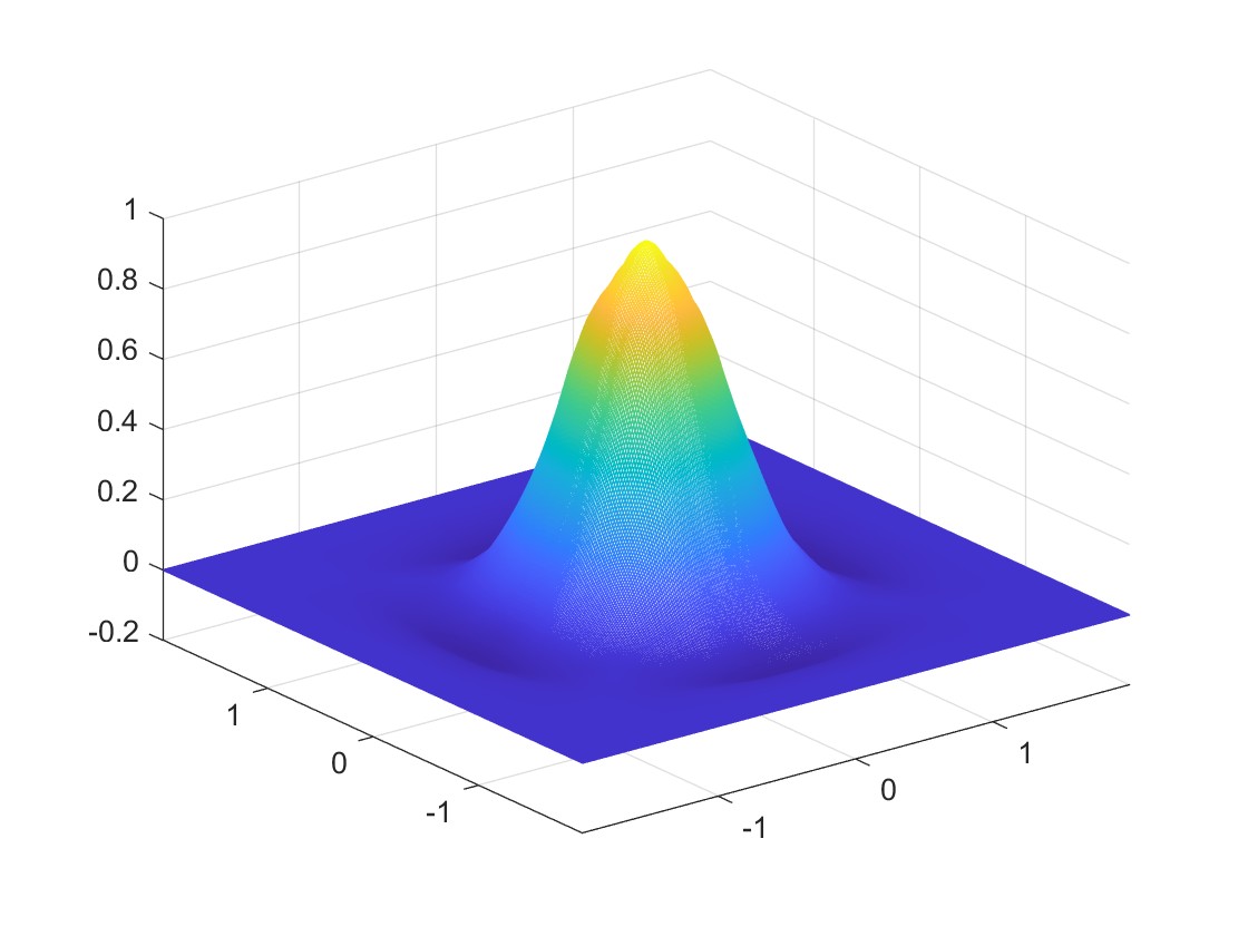
A $\phi\in\mathscr{C}^{1}(\mathbb{R}^{2})$

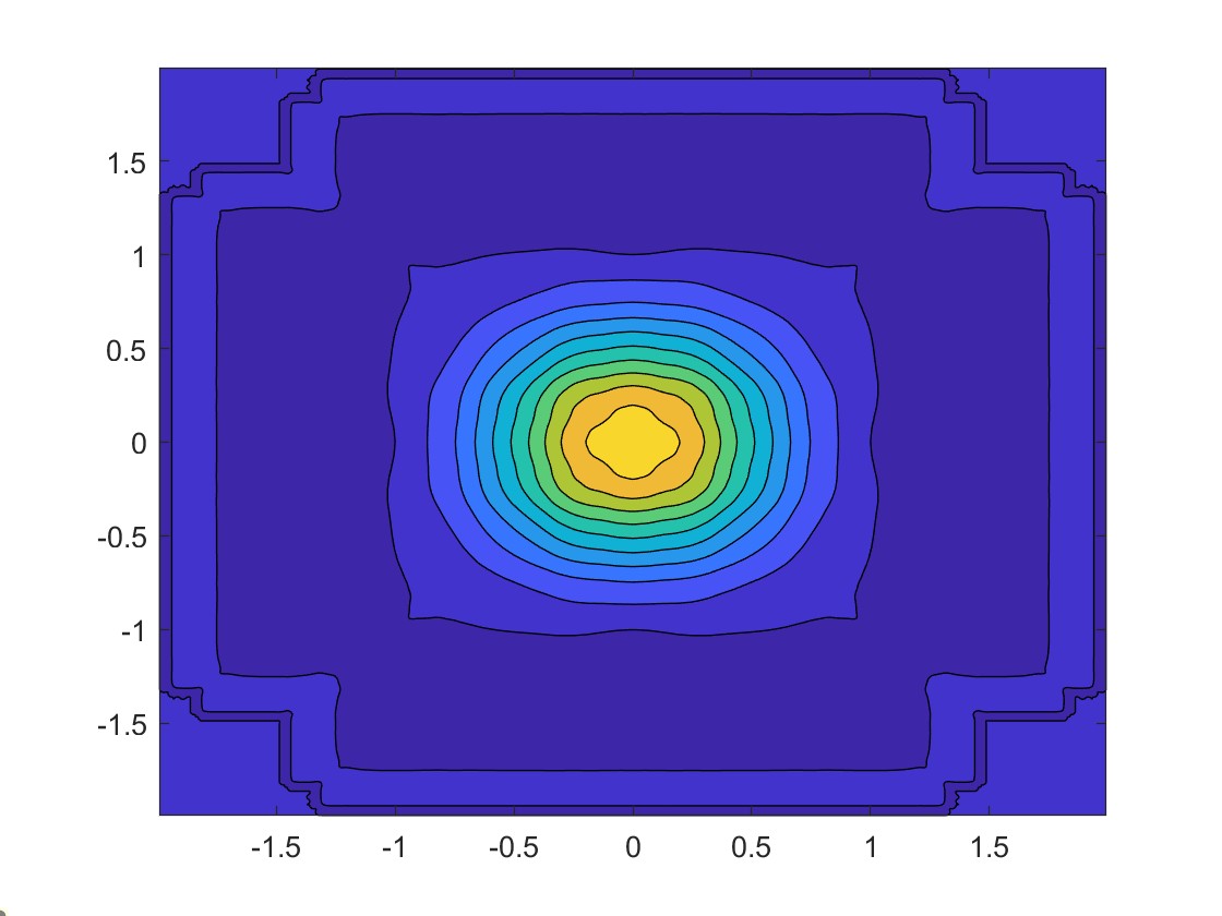
B Contour of $\phi$

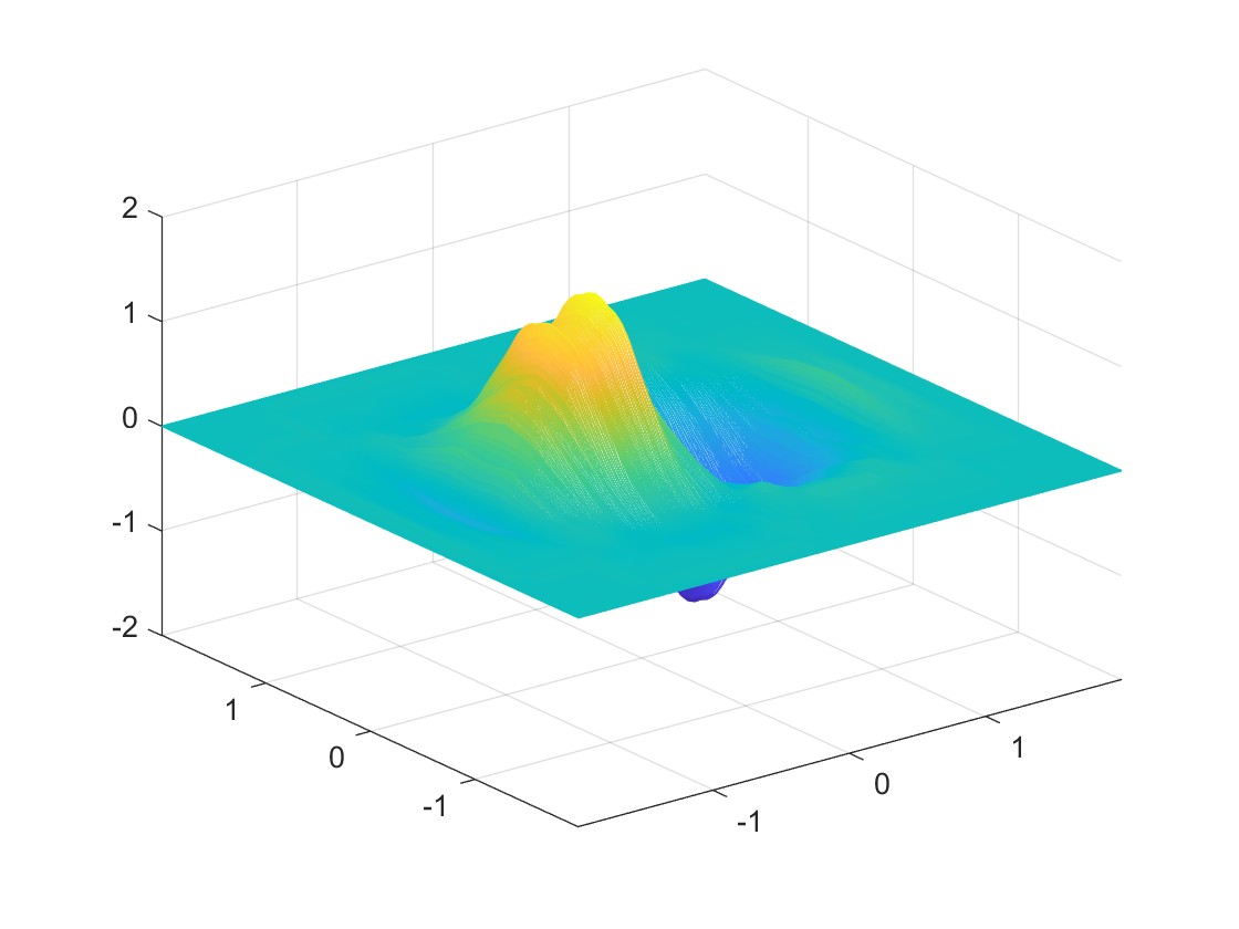
C $\frac{\partial\phi}{\partial x}\in C^{0}(\mathbb{R}^{2})$

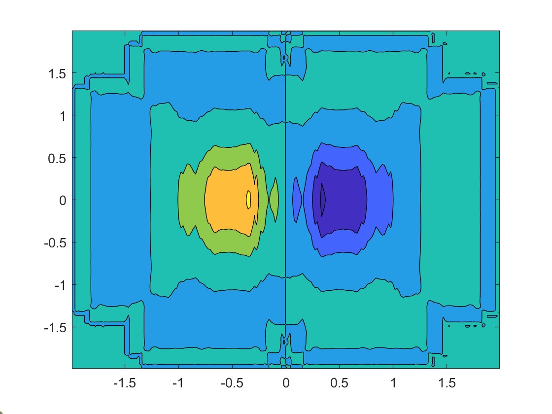
D Contour of $\frac{\partial\phi}{\partial x}$

Figure 1. (A) is the graph of the interpolating $4I_{2}$-refinable function $\phi\in C^{1}(\mathbb{R}^{2})$ in Example 1 and (B) is its contour. (C) is the graph of the partial derivative $\frac{\partial\phi}{\partial x}\in C^{0}(\mathbb{R}^{2})$, and (D) is the contour of $\frac{\partial\phi}{\partial x}$.

Let $\mathcal{G}=D_{6}$ and parameterize two masks $a_{1},a_{2}\in l_{0}(\mathbb{Z}^{2})$ such that

• $\widehat{a_{1}}(0)=\widehat{a_{2}}(0)=1$, $\operatorname{sr}(a_{1},2I_{2})=\operatorname{sr}(a_{2},2I_{2})=2$;

• $a_{1}$ and $a_{2}$ have $1$-ring stencil;

• $a_{1}$ and $a_{2}$ are $D_{6}$-symmetric about $(0,0)$;

as follows

$$\widehat{a_{1}}(\xi_{1},\xi_{2}):=\frac{1}{8}(1+e^{-i\xi_{1}})(1+e^{-i\xi_{2}})(1+e^{i(\xi_{1}+\xi_{2})})(t_{1}\widehat{p}(\xi_{1},\xi_{2})+1),$$ (3.17)

$$\widehat{a_{2}}(\xi_{1},\xi_{2}):=\frac{1}{8}(1+e^{-i\xi_{1}})(1+e^{-i\xi_{2}})(1+e^{i(\xi_{1}+\xi_{2})})(t_{2}\widehat{p}(\xi_{1},\xi_{2})+1),$$ (3.18)

where $t_{1},t_{2}$ are free parameters and $p\in l_{0}(\mathbb{Z}^{2})$ is given by

$$\widehat{p}(\xi):=e^{-i\xi_{1}}+e^{i\xi_{1}}+e^{-i\xi_{2}}+e^{i\xi_{2}}+e^{-i(\xi_{1}+\xi_{2})}+e^{i(\xi_{1}+\xi_{2})}-6.$$ (3.19)

Define the mask $a\in l_{0}(\mathbb{Z}^{2})$ via (3.8) with the above masks $a_{1},a_{2}\in l_{0}(\mathbb{Z}^{2})$ and we estimate $\operatorname{sm}_{\infty}(a,4I_{2})$. Since (3.11) must hold for all $u\in l_{0}(\mathbb{Z}^{2})$ and $E=\begin{bmatrix}0&1\\ 1&0\end{bmatrix}\in D_{6}$, it is easy to see that (3.13) must hold. For every $u\in l_{0}(\mathbb{Z}^{2})$ and $k\in\mathbb{Z}^{2}$, we have

$$\nabla_{e_{1}}u(k)=u(k)-u(k+e_{2})+u(k+e_{2})-u(k-e_{1})=-\nabla_{e_{2}}u(k+e_{2})+\nabla_{e_{1}+e_{2}}u(k+e_{2}).$$ (3.20)

Hence

$$\left\|\nabla^{(2,0)}\mathcal{S}_{a,4I_{2}}^{n}\boldsymbol{\delta}\right\|_{l_{\infty}(\mathbb{Z}^{2})} =\left\|\nabla_{e_{1}}^{2}\mathcal{S}_{a,4I_{2}}^{n}\boldsymbol{\delta}\right\|_{l_{\infty}(\mathbb{Z}^{2})}\leqslant\left\|\nabla_{e_{1}}\nabla_{e_{2}}\mathcal{S}_{a,4I_{2}}^{n}\boldsymbol{\delta}\right\|_{l_{\infty}(\mathbb{Z}^{2})}+\left\|\nabla_{e_{1}}\nabla_{e_{1}+e_{2}}\mathcal{S}_{a,4I_{2}}^{n}\boldsymbol{\delta}\right\|_{l_{\infty}(\mathbb{Z}^{2})}$$

$$\leqslant 2\max\left\{\left\|\nabla_{e_{1}}\nabla_{e_{2}}\mathcal{S}_{a,4I_{2}}^{n}\boldsymbol{\delta}\right\|_{l_{\infty}(\mathbb{Z}^{2})},\,\left\|\nabla_{e_{1}}\nabla_{e_{1}+e_{2}}\mathcal{S}_{a,4I_{2}}^{n}\boldsymbol{\delta}\right\|_{l_{\infty}(\mathbb{Z}^{2})}\right\},$$

and thus

$$\rho_{2}(a,4I_{2},(2,0))_{\infty}\leqslant\max\left\{\lim_{n\to\infty}\left\|\nabla_{e_{1}}\nabla_{e_{2}}\mathcal{S}_{a,4I_{2}}^{n}\boldsymbol{\delta}\right\|_{l_{\infty}(\mathbb{Z}^{2})}^{\frac{1}{n}},\,\lim_{n\to\infty}\left\|\nabla_{e_{1}}\nabla_{e_{1}+e_{2}}\mathcal{S}_{a,4I_{2}}^{n}\boldsymbol{\delta}\right\|_{l_{\infty}(\mathbb{Z}^{2})}^{\frac{1}{n}}\right\}.$$

Moreover, as $E=\begin{bmatrix}1&-1\\ 0&-1\end{bmatrix}\in D_{6}$, the $D_{6}$-symmetry of $\mathcal{S}_{a,4I_{2}}^{n}\boldsymbol{\delta}$ yields

$$\left\|\nabla_{e_{1}}\nabla_{e_{2}}\mathcal{S}_{a,4I_{2}}^{n}\boldsymbol{\delta}\right\|_{l_{\infty}(\mathbb{Z}^{2})}=\left\|\nabla_{E^{-1}e_{1}}\nabla_{E^{-1}e_{2}}\mathcal{S}_{a,4I_{2}}^{n}\boldsymbol{\delta}\right\|_{l_{\infty}(\mathbb{Z}^{2})}=\left\|\nabla_{e_{1}}\nabla_{e_{1}+e_{2}}\mathcal{S}_{a,4I_{2}}^{n}\boldsymbol{\delta}\right\|_{l_{\infty}(\mathbb{Z}^{2})}.$$ (3.21)

Therefore, it follows that

$$\rho_{2}(a,4I_{2},(2,0))_{\infty}\leqslant\lim_{n\to\infty}\left\|\nabla_{e_{1}}\nabla_{e_{2}}\mathcal{S}_{a,4I_{2}}^{n}\boldsymbol{\delta}\right\|_{l_{\infty}(\mathbb{Z}^{2})}^{\frac{1}{n}}=\rho_{2}(a,4I_{2},(1,1))_{\infty},$$

which further implies that

$$\rho_{2}(a,4I_{2})_{\infty}=\rho_{2}(a,4I_{2},(1,1))_{\infty}.$$

Let $p\in l_{0}(\mathbb{Z}^{2})$ be the same as in (3.19). Define $b\in l_{0}(\mathbb{Z}^{2})$ via

$$\widehat{b}(\xi):=\frac{1}{64}(1+e^{i(\xi_{1}+\xi_{2})})(1+e^{2i(\xi_{1}+\xi_{2})})(t_{1}\widehat{p}(2\xi)+1)(t_{2}\widehat{p}(\xi)+1).$$ (3.22)

Note that

$$\widehat{a}(\xi_{1},\xi_{2})=\frac{\widehat{\nabla^{(1,1)}\boldsymbol{\delta}}(4\xi_{1},4\xi_{2})}{\widehat{\nabla^{(1,1)}\boldsymbol{\delta}}(\xi_{1},\xi_{2})}\widehat{b}(\xi_{1},\xi_{2}),$$

We then conclude from Theorems 6 and  7 that

$$\rho_{2}(a,4I_{2},(1,1))_{\infty}=\lim_{n\to\infty}\left\|\mathcal{S}_{b,4I_{2}}^{n}\boldsymbol{\delta}\right\|_{l_{\infty}(\mathbb{Z}^{2})}^{\frac{1}{n}}\leqslant\left(\sup_{\gamma\in\Gamma_{4^{n}}}\sum_{k\in\mathbb{Z}^{d}}\left|\mathcal{S}_{b,4I_{2}}^{n}\boldsymbol{\delta}(\gamma+\mathsf{M}^{n}k)\right|\right)^{\frac{1}{n}},\quad\forall n\in\mathbb{N}.$$

Consequently, we obtain

$$\operatorname{sm}_{\infty}(a,4I_{2})\geqslant-\log_{4}\left(\sup_{\gamma\in\Gamma_{4^{n}}}\sum_{k\in\mathbb{Z}^{2}}\left|\mathcal{S}_{b,4I_{2}}^{n}\boldsymbol{\delta}(\gamma+4^{n}k)\right|\right)^{\frac{1}{n}},\qquad\forall n\in\mathbb{N},$$ (3.23)

where $b\in l_{0}(\mathbb{Z}^{2})$ is given by (3.22).

Example 2.

Let $a_{1},a_{2}\in l_{0}(\mathbb{Z}^{2})$ be given by (3.17) and (3.18) where $p\in l_{0}(\mathbb{Z}^{2})$ is given by (3.19) and $t_{1},t_{2}\in\mathbb{R}$ are free parameters. Define $a\in l_{0}(\mathbb{Z}^{2})$ via (3.8). By imposing the $4I_{2}$-interpolatory constraint $a(4k)=\frac{1}{16}\boldsymbol{\delta}(k)$ for all $k\in\mathbb{Z}^{2}$, we obtain $t_{1}=\frac{t_{2}}{2(2t_{2}-1)}$. By taking $t_{2}=\frac{11}{64}$, the masks $a_{1},a_{2}$ are then given by

$$a_{1}=\frac{1}{672}\begin{bmatrix}0&0&-11&-22&-11\\ 0&-22&106&106&-22\\ 11&106&234&106&-11\\ -22&106&106&-22&0\\ -11&-22&-11&0&0\end{bmatrix}_{[-2,2]^{2}},\quad a_{2}=\frac{1}{512}\begin{bmatrix}0&0&11&22&11\\ 0&22&42&42&22\\ 11&42&62&42&11\\ 22&42&42&22&0\\ 11&22&11&0&0\end{bmatrix}_{[-2,2]^{2}}.$$

Computation yields $\operatorname{sm}_{2}(a,4I_{2})\approx 1.709055$. Using the estimates in (3.23) with $n=1$, we obtain $\operatorname{sm}_{\infty}(a,4I_{2})\geqslant 1.30098$. Therefore, the $2$-mask interpolatory quasi-stationary $2I_{2}$-subdivision scheme using the masks $a_{1},a_{2}$ is $C^{1}$-convergent. See Figure 2 for the graphs of the standard $4I_{2}$-refinable function $\phi$ of the mask $a$, $\frac{\partial\phi}{\partial x}$, and the contours of $\phi$ and $\frac{\partial\phi}{\partial x}$.

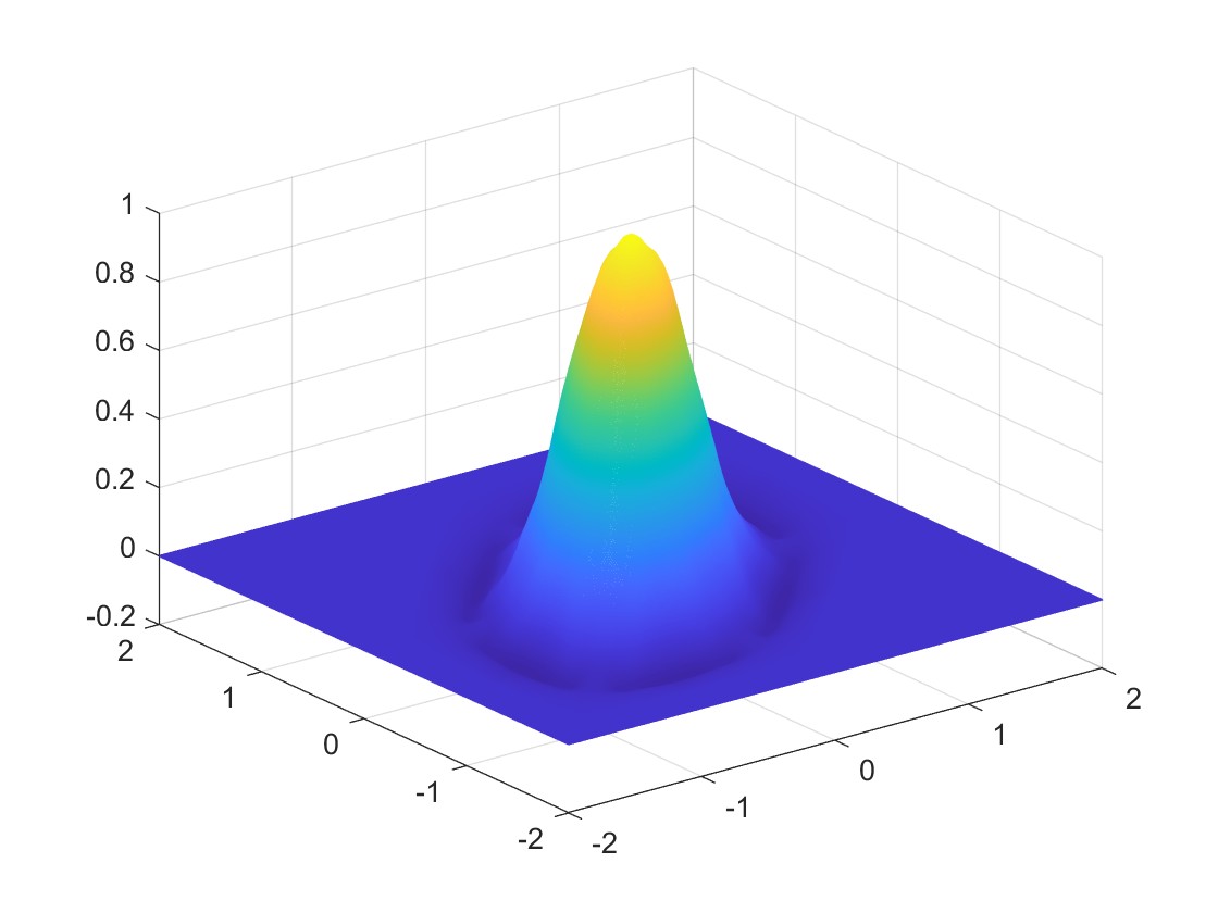
A $\phi\in\mathscr{C}^{1}(\mathbb{R}^{2})$

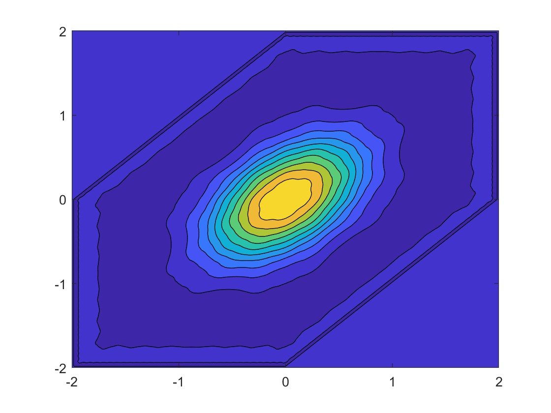
B Contour of $\phi$

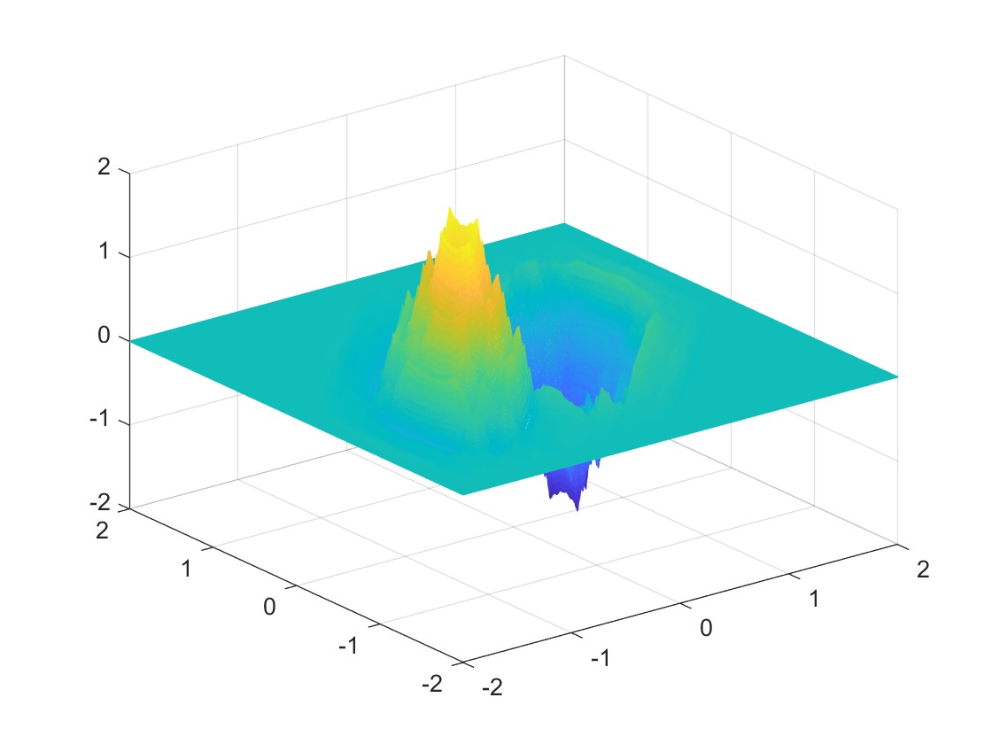
C $\frac{\partial\phi}{\partial x}\in C^{0}(\mathbb{R}^{2})$

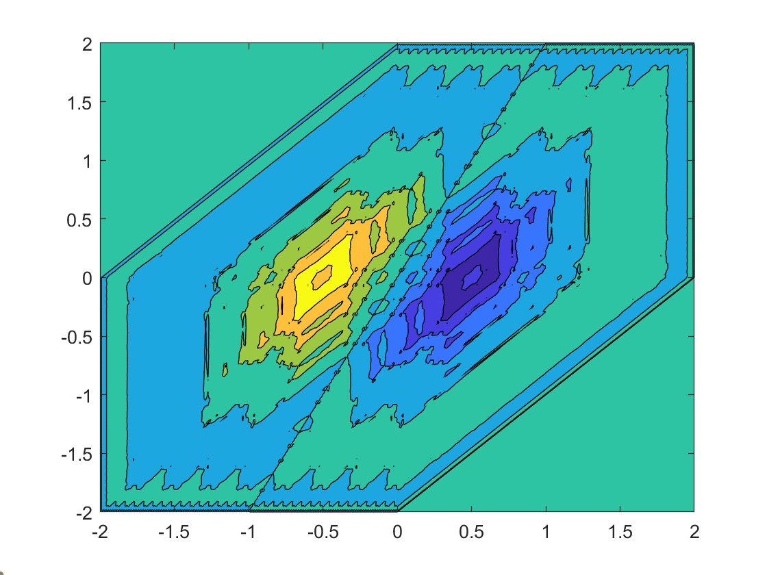
D Contour of $\frac{\partial\phi}{\partial x}$

Figure 2. (A) is the graph of the interpolating $4I_{2}$-refinable function $\phi\in C^{1}(\mathbb{R}^{2})$ in Example 2 and (B) is its contour. (C) is the graph of the partial derivative $\phi_{x}=\frac{\partial\phi}{\partial x}\in C^{0}(\mathbb{R}^{2})$, and (D) is the contour of $\frac{\partial\phi}{\partial x}$.

3.3. Examples of $C^{2}$-convergent schemes

Now we consider examples of $C^{2}$-convergent $r$-mask interpolatory quasi-stationary $2I_{2}$-subdivision schemes. We first observe that masks with $1$-ring stencil cannot achieve $C^{2}$-convergence. Indeed, suppose $a_{1},\dots,a_{r}\in l_{0}(\mathbb{Z}^{2})$ are $2I_{2}$-interpolatory and supported inside $[-2,2]^{2}$, then by [25, Theorem 3.4], we have $\operatorname{sr}(a_{l},2I_{2})\leqslant 2$ for all $l=1,\dots,r$. This implies that the mask $a:=2^{-2r}\mathcal{S}_{a_{r},2I_{2}}\dots\mathcal{S}_{a_{1},2I_{2}}\boldsymbol{\delta}$ is supported inside

$$(2^{r-1}+\dots+2+1)[-2,2]^{2}=[2-2^{r+1},2^{r+1}-2]^{2},$$

and satisfies $\operatorname{sr}(a,2^{r}I_{2})\leqslant 2$. Hence, by [25, Theorem 3.4] again yields $\operatorname{sm}_{\infty}(a,2^{r}I_{2})\leqslant 2$ and the standard $2^{r}I_{2}$-refinable function $\phi$ of the mask $a$ is not in $C^{2}(\mathbb{R}^{2})$, that is, the $r$-mask quasi-stationary $2I_{2}$-subdivision scheme that uses the masks $a_{1},\dots,a_{r}$ is not $C^{2}$-convergent. Consequently, a $C^{2}$-convergent interpolatory $r$-mask quasi-stationary $2I_{2}$-subdivision scheme must be at least $2$-ring stencils. Here we present $C^{2}$-convergent examples with $r=2$.

Let $\mathcal{G}=D_{4}$ and parameterize two masks $a_{1},a_{2}\in l_{0}(\mathbb{Z}^{2})$ such that

• $\widehat{a_{1}}(0)=\widehat{a_{2}}(0)=1$, $\operatorname{sr}(a_{1},2I_{2})=\operatorname{sr}(a_{2},2I_{2})=4$;

• $a_{1}$ and $a_{2}$ have $2$-ring stencil;

• $a_{1}$ and $a_{2}$ are $D_{4}$-symmetric about $(0,0)$;

as follows:

$$\widehat{a_{1}}(\xi_{1},\xi_{2}):=\frac{1}{256}e^{2i(\xi_{1}+\xi_{2})}(1+e^{-i\xi_{1}})^{4}(1+e^{-i\xi_{2}})^{4}\widehat{p_{1}}(\xi_{1},\xi_{2}),$$ (3.24)

$$\widehat{a_{2}}(\xi_{1},\xi_{2}):=\frac{1}{256}e^{2i(\xi_{1}+\xi_{2})}(1+e^{-i\xi_{1}})^{4}(1+e^{-i\xi_{2}})^{4}\widehat{p_{2}}(\xi_{1},\xi_{2}),$$ (3.25)

where $t_{1},\ldots,t_{8}\in\mathbb{R}$ are free parameters and $p_{1},p_{2}\in l_{0}(\mathbb{Z}^{2})$ are given by

$$p_{1}=\begin{bmatrix}t_{5}&t_{4}&t_{3}&t_{4}&t_{5}\\ t_{4}&t_{2}&t_{1}&t_{2}&t_{4}\\ t_{3}&t_{1}&1-4t_{1}-4t_{5}-4t_{3}-8t_{4}-4t_{2}&t1&t_{3}\\ t_{4}&t_{2}&t_{1}&t_{2}&t_{4}\\ t_{5}&t_{4}&t_{3}&t_{4}&t_{5}\end{bmatrix}_{[-2,2]^{2}},$$ (3.26)

and

$$p_{2}=\begin{bmatrix}0&0&t_{8}&0&0\\ 0&t_{7}&t_{6}&t_{7}&t_{0}\\ t_{8}&t_{6}&1-4t_{6}-4t_{7}-4t_{8}&t6&t_{8}\\ 0&t_{7}&t_{6}&t_{7}&0\\ 0&0&t_{8}&0&0\end{bmatrix}_{[-2,2]^{2}}.$$ (3.27)

Define $a\in l_{0}(\mathbb{Z}^{2})$ via (3.8) with $a_{1},a_{2}\in l_{0}(\mathbb{Z}^{2})$ being given by (3.24) and (3.25). To estimate $\operatorname{sm}_{\infty}(a,4I_{2})$, it suffices to estimate

$$\rho_{4}(a,4I_{2},\mu)_{\infty}:=\lim_{n\to\infty}\left\|\nabla^{\mu}\mathcal{S}_{a,4I_{2}}^{n}\boldsymbol{\delta}\right\|_{e_{\infty}(\mathbb{Z}^{2})}^{\frac{1}{n}},\quad\text{for }\mu=(4,0),\,(3,1),\,(2,2),\,(1,3),\,(0,4).$$

Since $a_{1},a_{2}$ are $D_{4}$-symmetric, we have

$$\rho_{4}(a,4I_{2},(4,0))_{\infty}=\rho_{4}(a,4I_{2},(0,4))_{\infty},\quad\rho_{4}(a,4I_{2},(3,1))_{\infty}=\rho_{4}(a,4I_{2},(1,3))_{\infty},$$

so

$$\rho_{4}(a,4I_{2})_{\infty}=\max\{\rho_{4}(a,4I_{2},(4,0))_{\infty},\,\rho_{4}(a,4I_{2},(3,1))_{\infty},\,\rho_{4}(a,4I_{2},(2,2))_{\infty}\}.$$ (3.28)

For every $u\in l_{0}(\mathbb{Z}^{2})$ and $k\in\mathbb{Z}^{2}$, note that

$$\nabla_{e_{1}}\nabla_{e_{2}}u(k)=\nabla_{e_{2}}u(k)-\nabla_{e_{2}}u(k-e_{1}),\quad\nabla_{e_{2}}^{2}u(k)=\nabla_{e_{2}}u(k)-\nabla_{e_{2}}u(k-e_{2}),$$ (3.29)

from which we obtain

$$\rho_{4}(a,4I_{2},(3,1))_{\infty}=\lim_{n\to\infty}\left\|\nabla^{2}_{e_{1}}\nabla_{e_{1}}\nabla_{e_{2}}\mathcal{S}_{a,4I_{2}}^{n}\boldsymbol{\delta}\right\|_{l_{\infty}(\mathbb{Z}^{2})}^{\frac{1}{n}}\leqslant\lim_{n\to\infty}\left\|\nabla^{2}_{e_{1}}\nabla_{e_{2}}\mathcal{S}_{a,4I_{2}}^{n}\boldsymbol{\delta}\right\|_{l_{\infty}(\mathbb{Z}^{2})}^{\frac{1}{n}},$$ (3.30)

$$\rho_{4}(a,4I_{2},(2,2))_{\infty}=\lim_{n\to\infty}\left\|\nabla^{2}_{e_{1}}\nabla_{e_{2}}^{2}\mathcal{S}_{a,4I_{2}}^{n}\boldsymbol{\delta}\right\|_{l_{\infty}(\mathbb{Z}^{2})}^{\frac{1}{n}}\leqslant\lim_{n\to\infty}\left\|\nabla^{2}_{e_{1}}\nabla_{e_{2}}\mathcal{S}_{a,4I_{2}}^{n}\boldsymbol{\delta}\right\|_{l_{\infty}(\mathbb{Z}^{2})}^{\frac{1}{n}}.$$ (3.31)

Hence

$$\rho_{4}(a,4I_{2})_{\infty}\leqslant\max\left\{\rho_{4}(a,4I_{2},(4,0))_{\infty},\,\lim_{n\to\infty}\left\|\nabla^{2}_{e_{1}}\nabla_{e_{2}}\mathcal{S}_{a,4I_{2}}^{n}\boldsymbol{\delta}\right\|_{l_{\infty}(\mathbb{Z}^{2})}^{\frac{1}{n}}\right\}.$$

Let $p_{1},p_{2}\in l_{0}(\mathbb{Z}^{2})$ be given by (3.26) and (3.27). Define $h_{1},h_{2}\in l_{0}(\mathbb{Z}^{2})$ via

$$\widehat{h_{1}}(\xi_{1},\xi_{2}):=\frac{1}{65536}e^{6i(\xi_{1}+\xi_{2})}(1+e^{-i\xi_{2}})^{4}(1+e^{-2i\xi_{2}})^{4}\widehat{p_{1}}(2\xi_{1},2\xi_{2})\widehat{p_{2}}(\xi_{1},\xi_{2}),$$ (3.32)

$$\widehat{h_{2}}(\xi_{1},\xi_{2}):=\frac{1}{65536}e^{6i(\xi_{1}+\xi_{2})}(1+e^{-i\xi_{1}})^{2}(1+e^{-2i\xi_{1}})^{2}(1+e^{-i\xi_{2}})^{3}(1+e^{-2i\xi_{2}})^{3}\widehat{p_{1}}(2\xi_{1},2\xi_{2})\widehat{p_{2}}(\xi_{1},\xi_{2}).$$ (3.33)

Note that

$$\widehat{a}(\xi_{1},\xi_{2})=\frac{\widehat{\nabla^{(4,0)}\boldsymbol{\delta}}(4\xi_{1},4\xi_{2})}{\widehat{\nabla^{(4,0)}\boldsymbol{\delta}}(\xi_{1},\xi_{2})}\widehat{h_{1}}(\xi_{1},\xi_{2})=\frac{\widehat{\nabla^{2}_{e_{1}}\nabla_{e_{2}}\boldsymbol{\delta}}(4\xi_{1},4\xi_{2})}{\widehat{\nabla^{2}_{e_{1}}\nabla_{e_{2}}\boldsymbol{\delta}}(\xi_{1},\xi_{2})}\widehat{h_{2}}(\xi_{1},\xi_{2}).$$

We then conclude from Theorems 6 and  7 that

$$\rho_{4}(a,4I_{2},(4,0))_{\infty}=\lim_{n\to\infty}\left\|\mathcal{S}_{h_{1},4I_{2}}^{n}\boldsymbol{\delta}\right\|_{l_{\infty}(\mathbb{Z}^{2})}^{\frac{1}{n}}\leqslant\left(\sup_{\gamma\in\Gamma_{4^{n}}}\sum_{k\in\mathbb{Z}^{2}}\left|\mathcal{S}_{h_{1},4I_{2}}^{n}\boldsymbol{\delta}(\gamma+4^{n}k)\right|\right)^{\frac{1}{n}},$$

$$\lim_{n\to\infty}\left\|\nabla^{2}_{e_{1}}\nabla_{e_{2}}\mathcal{S}_{a,4I_{2}}^{n}\boldsymbol{\delta}\right\|_{l_{\infty}(\mathbb{Z}^{2})}^{\frac{1}{n}}=\lim_{n\to\infty}\left\|\mathcal{S}_{h_{2},4I_{2}}^{n}\boldsymbol{\delta}\right\|_{l_{\infty}(\mathbb{Z}^{2})}^{\frac{1}{n}}\leqslant\left(\sup_{\gamma\in\Gamma_{4^{n}}}\sum_{k\in\mathbb{Z}^{2}}\left|\mathcal{S}_{h_{2},4I_{2}}^{n}\boldsymbol{\delta}(\gamma+4^{n}k)\right|\right)^{\frac{1}{n}},$$

for all $n\in\mathbb{N}$. Consequently, we have

$$\operatorname{sm}_{\infty}(a,4I_{2})\geqslant-\log_{4}\left(\max_{j=1,2}\left(\sup_{\gamma\in\Gamma_{4^{n}}}\sum_{k\in\mathbb{Z}^{2}}\left|\mathcal{S}_{h_{j},4I_{2}}^{n}\boldsymbol{\delta}(\gamma+4^{n}k)\right|\right)^{\frac{1}{n}}\right),\quad\forall n\in\mathbb{N},$$ (3.34)

where $h_{1},h_{2}\in l_{0}(\mathbb{Z}^{2})$ are given by (3.32) and (3.33).

Example 3.

Let $p_{1},p_{2}\in l_{0}(\mathbb{Z}^{2})$ be given by (3.26) and (3.27) for some free parameters $t_{1},\dots,t_{8}\in\mathbb{R}$. Let $a_{1},a_{2}\in l_{0}(\mathbb{Z}^{2})$ be given by (3.24) and (3.25). Define $a\in l_{0}(\mathbb{Z}^{2})$ via (3.8). By imposing the $4I_{2}$-interpolatory constraint $a(4k)=\frac{1}{16}\boldsymbol{\delta}(k)$ for all $k\in\mathbb{Z}^{2}$, we have many solutions and here we present two solutions. The first choice is $t_{3}=t_{4}=t_{5}=0$, $t_{8}=t$, and

$$t_{1}=-\tfrac{90035}{1027628}t^{4}-\tfrac{21065363}{12331536}t^{3}+\tfrac{10201651}{3082884}t^{2}+\tfrac{13085857}{6165768}t-\tfrac{640565}{1541442},$$

$$t_{2}=-\tfrac{279697}{4110512}t^{4}-\tfrac{65258017}{49326144}t^{3}+\tfrac{16876337}{6165768}t^{2}+\tfrac{44294515}{12331536}t+\tfrac{2660345}{3082884},$$

$$t_{6}=\tfrac{1398881}{513814}t^{4}+\tfrac{325752977}{6165768}t^{3}-\tfrac{84880928}{770721}t^{2}-\tfrac{85869100}{770721}t-\tfrac{15771775}{770721},$$

$$t_{7}=-\tfrac{469557}{513814}t^{4}-\tfrac{36394039}{2055256}t^{3}+\tfrac{28901470}{770721}t^{2}+\tfrac{9016005}{256907}t+\tfrac{19610825}{3082884},$$

where $t\approx-0.2395777$ is a root of $132t^{5}+2651t^{4}-3600t^{3}-8896t^{2}-4560t-640=0$. We have

$$t_{1}\approx-0.71089031,\quad t_{2}\approx 0.17745551,\quad t_{6}\approx-0.810183,\quad t_{7}\approx 0.3462063,\quad t_{8}\approx-0.23957771.$$

The two masks $a_{1},a_{2}$ are then approximately given by

$$a_{1}={\begin{bmatrix}0.0006929244&-4.6872\times 10^{-6}&-0.0062550684&-0.0111149136&-0.0062550684&-4.6872\times 10^{-6}&0.0006929244\\ -4.6872\times 10^{-6}&0.0011210220&0.0045262728&0.0068011272&0.0045262728&0.0011210220&-4.6872\times 10^{-6}\\ -0.0062550684&0.0045262728&0.0744007068&0.1272387312&0.0744007068&0.0045262728&-0.0062550684\\ -0.0111149136&0.0068011272&0.1272387312&0.2186453808&0.1272387312&0.0068011272&-0.0111149136\\ -0.0062550684&0.0045262728&0.0744007068&0.1272387312&0.0744007068&0.0045262728&-0.0062550684\\ -4.6872\times 10^{-6}&0.0011210220&0.0045262728&0.0068011272&0.0045262728&0.0011210220&-4.6872\times 10^{-6}\\ 0.0006929244&-4.6872\times 10^{-6}&-0.0062550684&-0.0111149136&-0.0062550684&-4.6872\times 10^{-6}&0.0006929244\end{bmatrix}_{[-3,3]^{2}},}$$

$$a_{2}={\begin{bmatrix}0&0&-0.00093840&-0.00375360&-0.00563040&-0.00375360&-0.00093840&0&0\\ 0&0.0013294&-0.00234600&-0.02134860&-0.03534640&-0.02134860&-0.00234600&0.0013294&0\\ -0.00093840&-0.00234600&-0.00602140&-0.01798600&-0.02674440&-0.01798600&-0.00602140&-0.00234600&-0.00093840\\ -0.00375360&-0.02134860&-0.01798600&0.06013580&0.12105360&0.06013580&-0.01798600&-0.02134860&-0.00375360\\ -0.00563040&-0.03534640&-0.02674440&0.12105360&0.23616400&0.12105360&-0.02674440&-0.03534640&-0.00563040\\ -0.00375360&-0.02134860&-0.01798600&0.06013580&0.12105360&0.06013580&-0.01798600&-0.02134860&-0.00375360\\ -0.00093840&-0.00234600&-0.00602140&-0.01798600&-0.02674440&-0.01798600&-0.00602140&-0.00234600&-0.00093840\\ 0&0.0013294&-0.00234600&-0.02134860&-0.03534640&-0.02134860&-0.00234600&0.0013294&0\\ 0&0&-0.00093840&-0.00375360&-0.00563040&-0.00375360&-0.00093840&0&0\end{bmatrix}_{[-4,4]^{2}}.}$$

Moreover, direct computation yields $\operatorname{sm}_{2}(a,4I_{2})\approx 2.616519$. Using the estimation (3.34) with $n=2$, we obtain $\operatorname{sm}_{\infty}(a,4I_{2})\geqslant 2.07607$. Therefore, the $2$-mask interpolatory quasi-stationary $2I_{2}$-subdivision scheme using the above masks $a_{1},a_{2}$ is $C^{2}$-convergent.

Another choice is $t_{4}=0,t_{5}=-\tfrac{5}{128},t_{7}=\tfrac{t}{4},t_{8}=0$ and

$$t_{1}=\tfrac{424994944920607}{24908728622815420334080}t^{6}+\tfrac{7975356264181027}{9963491449126168133632}t^{5}-\tfrac{143174662095446521}{9963491449126168133632}t^{4}-\tfrac{201920022567847971491}{24908728622815420334080}t^{3}$$

$$\qquad-\tfrac{1877989942288756509}{6227182155703855083520}t^{2}-\tfrac{6489286410377804222101}{9963491449126168133632}t-\tfrac{26798558462517617887845}{9963491449126168133632},$$

$$t_{2}=\tfrac{113900026967}{77839776946298188544}t^{6}+\tfrac{6721822856723}{155679553892596377088}t^{5}-\tfrac{362570802099563}{155679553892596377088}t^{4}-\tfrac{52158296539168801}{77839776946298188544}t^{3}$$

$$\qquad+\tfrac{464437583880593005}{38919888473149094272}t^{2}-\tfrac{15627987102075198505}{155679553892596377088}t+\tfrac{203270998898608942625}{155679553892596377088},$$

$$t_{3}=-\tfrac{2633158952204571}{498174572456308406681600}t^{6}-\tfrac{46155986031448111}{199269828982523362672640}t^{5}+\tfrac{1033152943943700317}{199269828982523362672640}t^{4}+\tfrac{1243781358911040235183}{498174572456308406681600}t^{3}$$

$$\qquad-\tfrac{949630637866665816943}{124543643114077101670400}t^{2}+\tfrac{43309282197078887566441}{199269828982523362672640}t-\tfrac{3476955096904628746267}{39853965796504672534528},$$

$$t_{6}=\tfrac{561344301981}{121624651478590919600}t^{6}+\tfrac{7723586258751}{48649860591436367840}t^{5}-\tfrac{166473281489741}{24324930295718183920}t^{4}-\tfrac{262791785728360213}{121624651478590919600}t^{3}$$

$$\qquad+\tfrac{3373757083893137367}{121624651478590919600}t^{2}-\tfrac{27687970920178103501}{48649860591436367840}t+\tfrac{2232880122164793821}{4864986059143636784},$$

where $t\approx 2.233641927$ is a root of

$$2t^{7}+95t^{6}-1660t^{5}-952671t^{4}-573006t^{3}-61196575t^{2}-340415800t+1095865375=0.$$

We have

$$t_{1}\approx-4.2366142,\quad t_{2}\approx 1.1334896,\quad t_{3}\approx 0.38811383,\quad t_{6}\approx-0.69810232,\quad t_{7}\approx 0.55841048,$$

and the masks $a_{1},a_{2}$ are approximately given by

$$a_{1}={\begin{bmatrix}-0.0001521&-0.0006084&0.0005694&0.0053196&0.0085878&0.0053196&0.0005694&-0.0006084&-0.0001521\\ -0.0006084&0.0018564&0.0030576&-0.0142116&-0.0296088&-0.0142116&0.0030576&0.0018564&-0.0006084\\ 0.0005694&0.0030576&-0.0032916&-0.0315744&-0.0515892&-0.0315744&-0.0032916&0.0030576&0.0005694\\ 0.0053196&-0.0142116&-0.0315744&0.0867204&0.1975272&0.0867204&-0.0315744&-0.0142116&0.0053196\\ 0.0085878&-0.0296088&-0.0515892&0.1975272&0.4218396&0.1975272&-0.0515892&-0.0296088&0.0085878\\ 0.0053196&-0.0142116&-0.0315744&0.0867204&0.1975272&0.0867204&-0.0315744&-0.0142116&0.0053196\\ 0.0005694&0.0030576&-0.0032916&-0.0315744&-0.0515892&-0.0315744&-0.0032916&0.0030576&0.0005694\\ -0.0006084&0.0018564&0.0030576&-0.0142116&-0.0296088&-0.0142116&0.0030576&0.0018564&-0.0006084\\ -0.0001521&-0.0006084&0.0005694&0.0053196&0.0085878&0.0053196&0.0005694&-0.0006084&-0.0001521\end{bmatrix}_{[-4,4]^{2}},}$$

$$a_{2}={\begin{bmatrix}0.002145&0.005694&0.003471&-0.000156&0.003471&0.005694&0.002145\\ 0.005694&0.017862&0.020202&0.016068&0.020202&0.017862&0.005694\\ 0.003471&0.020202&0.049569&0.065676&0.049569&0.020202&0.003471\\ -0.000156&0.016068&0.065676&0.098904&0.065676&0.016068&-0.000156\\ 0.003471&0.020202&0.049569&0.065676&0.049569&0.020202&0.003471\\ 0.005694&0.017862&0.020202&0.016068&0.020202&0.017862&0.005694\\ 0.002145&0.005694&0.003471&-0.000156&0.003471&0.005694&0.002145\end{bmatrix}_{[-3,3]^{2}}.}$$

Moreover, direct computation yields $\operatorname{sm}_{2}(a,4I_{2})\approx 3.074404$. Hence, using (1.13) we obtain $\operatorname{sm}_{\infty}(a,4I_{2})\geqslant 2.074404$. Therefore, the $2$-mask interpolatory quasi-stationary $2I_{2}$-subdivision scheme using the above masks $a_{1},a_{2}$ is $C^{2}$-convergent. See Figure 3 for the graphs of the $4I_{2}$-standard refinable function $\phi$ of the mask $a$ with the second choice, $\frac{\partial^{2}\phi}{\partial x^{2}}$, and the contours of $\phi$ and $\frac{\partial^{2}\phi}{\partial x^{2}}$.

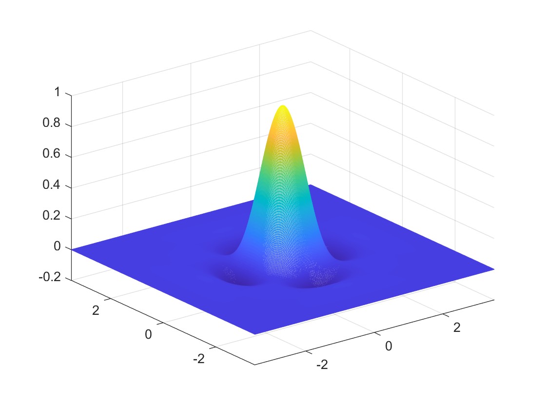
A $\phi\in\mathscr{C}^{2}(\mathbb{R}^{2})$

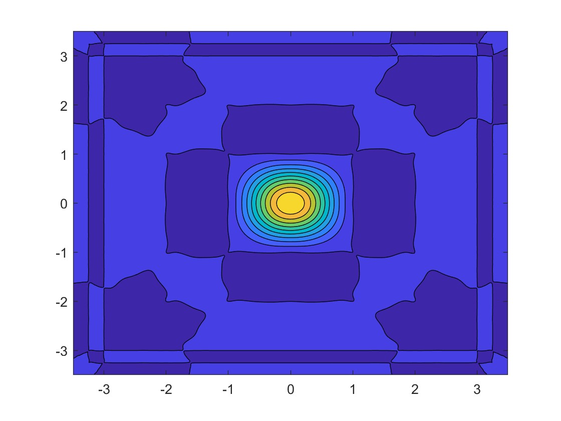
B Contour of $\phi$

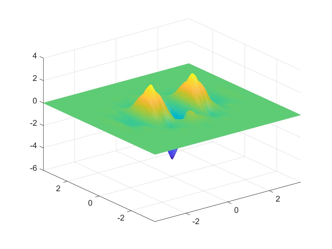
C $\frac{\partial^{2}\phi}{\partial x^{2}}\in C^{0}(\mathbb{R}^{2})$

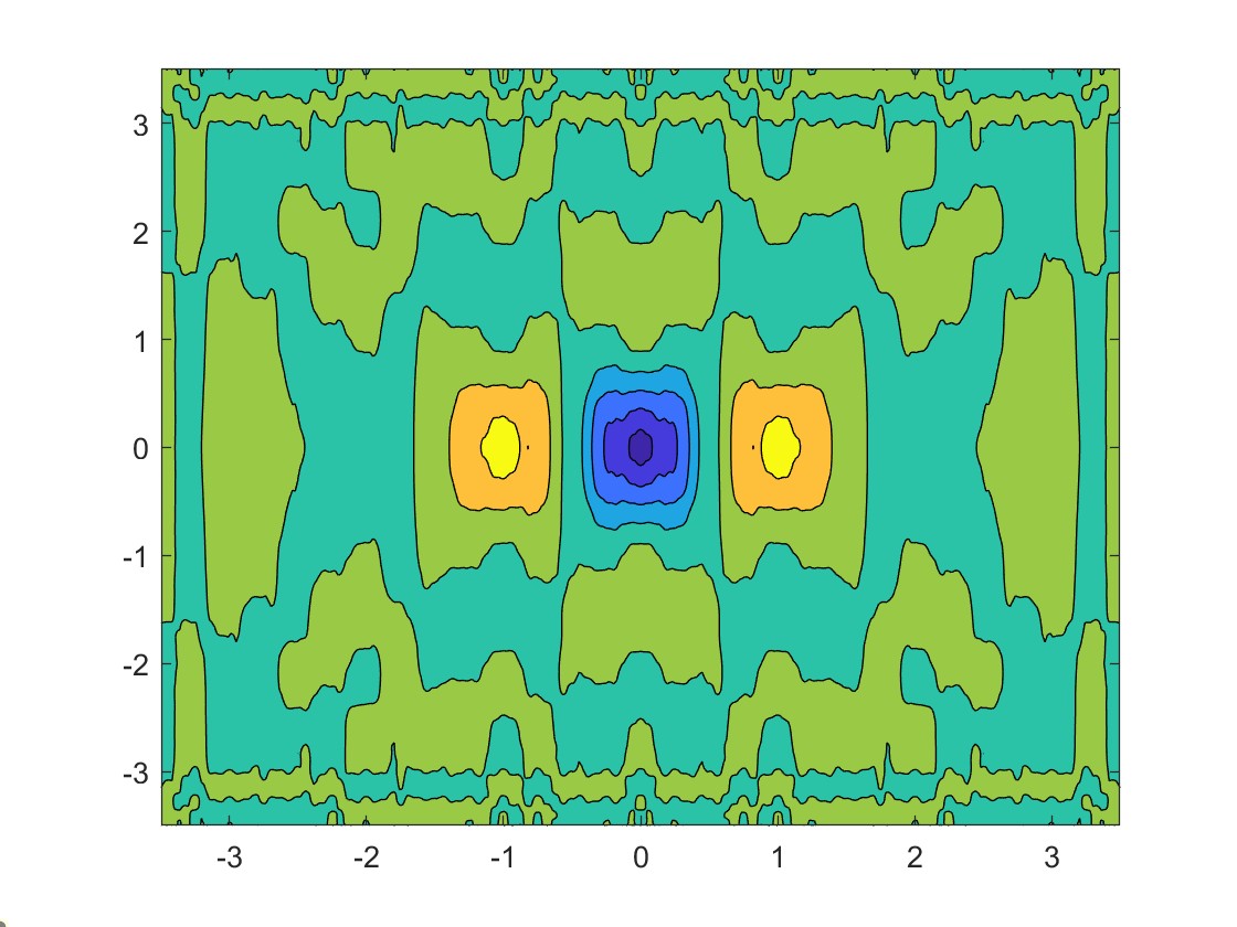
D Contour of $\frac{\partial^{2}\phi}{\partial x^{2}}$

Figure 3. (A) is the graph of the interpolating $4I_{2}$-refinable function $\phi\in C^{2}(\mathbb{R}^{2})$ in Example 3 and (B) is its contour. (C) is the graph of the partial derivative $\frac{\partial^{2}\phi}{\partial x^{2}}\in C^{0}(\mathbb{R}^{2})$, and (D) is the contour of $\frac{\partial^{2}\phi}{\partial x^{2}}$.

Let $\mathcal{G}=D_{6}$ and parameterize two masks $a_{1},a_{2}\in l_{0}(\mathbb{Z}^{2})$ such that

• $\widehat{a_{1}}(0)=\widehat{a_{2}}(0)=1$, $\operatorname{sr}(a_{1},2I_{2})=\operatorname{sr}(a_{2},2I_{2})=4$;

• $a_{1}$ and $a_{2}$ have two-ring stencils;

• $a_{1}$ and $a_{2}$ are $D_{6}$-symmetric about $(0,0)$;

as follows:

$$\widehat{a_{1}}(\xi_{1},\xi_{2}):=\frac{1}{64}(1+e^{-i\xi_{1}})^{2}(1+e^{-i\xi_{2}})^{2}(1+e^{i(\xi_{1}+\xi_{2})})^{2}\widehat{g_{1}}(\xi_{1},\xi_{2}),$$ (3.35)

$$\widehat{a_{2}}(\xi_{1},\xi_{2}):=\frac{1}{64}(1+e^{-i\xi_{1}})^{2}(1+e^{-i\xi_{2}})^{2}(1+e^{i(\xi_{1}+\xi_{2})})^{2}\widehat{g_{2}}(\xi_{1},\xi_{2}),$$ (3.36)

where $g_{1},g_{2}\in l_{0}(\mathbb{Z}^{2})$ are given by

$$g_{1}=\begin{bmatrix}0&0&t_{3}&t_{2}&t_{3}\\ 0&t_{2}&t_{1}&t_{1}&t_{2}\\ t_{3}&t_{1}&1-6t_{3}-6t_{2}-6t_{1}&t_{1}&t_{3}\\ t_{2}&t_{1}&t_{1}&t_{2}&0\\ t_{3}&t_{2}&t_{3}&0&0\end{bmatrix}_{[-2,2]^{2}},\quad g_{2}=\begin{bmatrix}0&0&t_{6}&t_{5}&t_{6}\\ 0&t_{5}&t_{4}&t_{4}&t_{5}\\ t_{6}&t_{4}&1-6t_{6}-6t_{5}-6t_{4}&t_{4}&t_{6}\\ t_{5}&t_{4}&t_{4}&t_{5}&0\\ t_{6}&t_{5}&t_{6}&0&0\end{bmatrix}_{[-2,2]^{2}},$$ (3.37)

where $t_{1},\dots,t_{6}\in\mathbb{R}$ are free parameters. Define $a\in l_{0}(\mathbb{Z}^{2})$ via (3.8). Since $a_{1},a_{2}$ are $D_{6}$-symmetric about $(0,0)$, it is easy to see that (3.28) holds. By letting $E=\begin{bmatrix}1&-1\\ 0&-1\end{bmatrix}\in D_{6}$, (3.21) holds, which together with (3.20), yields $\rho_{4}(a,4I_{2},(4,0))_{\infty}\leqslant\rho_{4}(a,4I_{2},(3,1))_{\infty}.$ Furthermore, one can conclude from (3.29) that (3.30) and (3.31) must hold. Therefore, we have

$$\rho_{4}(a,4I_{2})_{\infty}\leqslant\lim_{n\to\infty}\left\|\nabla^{2}_{e_{1}}\nabla_{e_{2}}\mathcal{S}_{a,4I_{2}}^{n}\boldsymbol{\delta}\right\|_{l_{\infty}(\mathbb{Z}^{2})}^{\frac{1}{n}}.$$

Let $g_{1},g_{2}\in\l_{0}(\mathbb{Z}^{2})$ be given by (3.37). Define $h\in l_{0}(\mathbb{Z}^{2})$ via

$$\widehat{h}(\xi_{1},\xi_{2})=\frac{1}{4096}(1+e^{-i\xi_{2}})(1+e^{-2i\xi_{2}})(1+e^{i(\xi_{1}+\xi_{2})})^{2}(1+e^{2i(\xi_{1}+\xi_{2})})^{2}\widehat{g_{1}}(2\xi_{1},2\xi_{2})\widehat{g_{2}}(\xi_{1},\xi_{2}).$$ (3.38)

Note that

$$\widehat{a}(\xi_{1},\xi_{2})=\frac{\widehat{\nabla^{2}_{e_{1}}\nabla_{e_{2}}\boldsymbol{\delta}}(4\xi_{1},4\xi_{2})}{\widehat{\nabla^{2}_{e_{1}}\nabla_{e_{2}}\boldsymbol{\delta}}(\xi_{1},\xi_{2})}\widehat{h}(\xi_{1},\xi_{2}).$$

It then follows from Theorems 6 and  7 that

$$\lim_{n\to\infty}\left\|\nabla^{2}_{e_{1}}\nabla_{e_{2}}\mathcal{S}_{a,4I_{2}}^{n}\boldsymbol{\delta}\right\|_{l_{\infty}(\mathbb{Z}^{2})}^{\frac{1}{n}}=\lim_{n\to\infty}\left\|\mathcal{S}_{h,4I_{2}}^{n}\boldsymbol{\delta}\right\|_{l_{\infty}(\mathbb{Z}^{2})}^{\frac{1}{n}}\leqslant\left(\sup_{\gamma\in\Gamma_{4^{n}}}\sum_{k\in\mathbb{Z}^{2}}\left|\mathcal{S}_{h,4I_{2}}^{n}\boldsymbol{\delta}(\gamma+4^{n}k)\right|\right)^{\frac{1}{n}},\quad\forall n\in\mathbb{N}.$$

Consequently, we have

$$\operatorname{sm}_{\infty}(a,4I_{2})\geqslant-\log_{4}\left(\sup_{\gamma\in\Gamma_{4^{n}}}\sum_{k\in\mathbb{Z}^{2}}\left|\mathcal{S}_{h,4I_{2}}^{n}\boldsymbol{\delta}(\gamma+4^{n}k)\right|\right)^{\frac{1}{n}},\quad\forall n\in\mathbb{N},$$ (3.39)

where $h\in l_{0}(\mathbb{Z}^{2})$ is given by (3.38).

Example 4.

Let $g_{1},g_{2}\in l_{0}(\mathbb{Z}^{2})$ be given by (3.37) where $t_{1},\dots,t_{6}\in\mathbb{R}$ are free parameters. Define $a_{1},a_{2}\in l_{0}(\mathbb{Z}^{2})$ via (3.35) and (3.36) and define $a\in l_{0}(\mathbb{Z}^{2})$ via (3.8). By imposing the $4I_{2}$-interpolatory constraint $a(4k)=\frac{1}{16}\boldsymbol{\delta}(k)$ for all $k\in\mathbb{Z}^{2}$, we have many solutions and here we present two solutions. The first choice is

$$t_{1}=-\frac{5}{8},\quad t_{2}=\frac{5}{48},\quad t_{3}=t_{4}=t_{5}=t_{6}=0.$$

The two masks $a_{1},a_{2}$ are then given by

$$a_{1}=\frac{1}{3072}\begin{bmatrix}0&0&0&0&0&5&10&5&0\\ 0&0&0&5&-10&-55&-55&-10&5\\ 0&0&10&-55&-42&46&-42&-55&10\\ 0&5&-55&46&448&448&46&-55&5\\ 0&-10&-42&448&960&448&-42&-10&0\\ 5&-55&46&448&448&46&-55&5&0\\ 10&-55&-42&46&-42&-55&10&0&0\\ 5&-10&-55&-55&-10&5&0&0&0\\ 0&5&10&5&0&0&0&0&0\end{bmatrix}_{[-4,4]^{2}},$$

$$a_{2}=\frac{1}{64}\begin{bmatrix}0&0&1&2&1\\ 0&2&6&6&2\\ 1&6&10&6&1\\ 2&6&6&2&0\\ 1&2&1&0&0\end{bmatrix}_{[-2,2]^{2}}.$$

Computaiton yields $\operatorname{sm}_{2}(a,4I_{2})\approx 2.653820$. Using the estimation (3.39) with $n=2$, we obtain $\operatorname{sm}_{\infty}(a,4I_{2})\geqslant 2.06210$. Therefore, the $2$-mask interpolatory quasi-stationary $2$-subdivision scheme using the above masks $a_{1},a_{2}$ is $C^{2}$-convergent. See the first row of Figure 4 for the graphs of the standard $4I_{2}$-refinable function $\phi$ of the mask $a$, $\frac{\partial^{2}\phi}{\partial x^{2}}$ and the contours of $\phi$ and $\phi_{xx}$.

Another choice is

$$t_{1}=-\tfrac{2t^{2}}{7}-\tfrac{145t}{112}-\tfrac{151}{112},\quad t_{2}=\tfrac{2t^{2}}{21}+\tfrac{131t}{336}+\tfrac{109}{336},\quad t_{3}=0,\quad t_{4}=\tfrac{t}{2},\quad t_{5}=\tfrac{1}{4},\quad t_{6}=-\tfrac{1}{8},$$

where $t\approx-0.133008$ is a root of $32t^{3}+141t^{2}+146t+17=0$. The two masks $a_{1},a_{2}$ are then approximately given by

$$a_{1}={\begin{bmatrix}0&0&0&0&0&0.0042744&0.0085488&0.0042744&0\\ 0&0&0&0.0042744&-0.0013104&-0.0253032&-0.0253032&-0.0013104&0.0042744\\ 0&0&0.0085488&-0.0253032&-0.0323232&0.0030576&-0.0323232&-0.0253032&0.0085488\\ 0&0.0042744&-0.0253032&0.0030576&0.1656096&0.1656096&0.0030576&-0.0253032&0.0042744\\ 0&-0.0013104&-0.0323232&0.1656096&0.3932448&0.1656096&-0.0323232&-0.0013104&0\\ 0.0042744&-0.0253032&0.0030576&0.1656096&0.1656096&0.0030576&-0.0253032&0.0042744&0\\ 0.0085488&-0.0253032&-0.0323232&0.0030576&-0.0323232&-0.0253032&0.0085488&0&0\\ 0.0042744&-0.0013104&-0.0253032&-0.0253032&-0.0013104&0.0042744&0&0&0\\ 0&0.0042744&0.0085488&0.0042744&0&0&0&0&0\end{bmatrix}_{[-4,4]^{2}},}$$

$$a_{2}={\begin{bmatrix}0,0&0&0&-0.0019500&0&0.0039000&0&-0.0019500\\ 0&0&0&0&0.00286260&0.00858780&0.00858780&0.00286260&0\\ 0&0&0.0039000&0.00858780&0.02315040&0.03692520&0.02315040&0.00858780&0.0039000\\ 0&0&0.00858780&0.03692520&0.06783660&0.06783660&0.03692520&0.00858780&0\\ -0.0019500&0.00286260&0.02315040&0.06783660&0.09899760&0.06783660&0.02315040&0.00286260&-0.0019500\\ 0&0.00858780&0.03692520&0.06783660&0.06783660&0.03692520&0.00858780&0&0\\ 0.0039000&0.00858780&0.02315040&0.03692520&0.02315040&0.00858780&0.0039000&0&0\\ 0&0.00286260&0.00858780&0.00858780&0.00286260&0&0&0&0\\ -0.0019500&0&0.0039000&0&-0.0019500&0&0&0&0\end{bmatrix}_{[-4,4]^{2}}.}$$

Moreover, computation yields $\operatorname{sm}_{2}(a,4I_{2})\approx 3.041495$ and the relation (1.13) yields $\operatorname{sm}_{\infty}(a,4I_{2})\geqslant 2.041495$. Therefore, the $2$-mask interpolatory quasi-stationary $2I_{2}$-subdivision scheme using the above masks $a_{1},a_{2}$ is $C^{2}$-convergent. See the second row of Figure 4 for the graphs of the standard $4I_{2}$-refinable function $\phi$ of the mask $a$, $\frac{\partial^{2}\phi}{\partial x^{2}}$, and the contours of $\phi$ and $\frac{\partial^{2}\phi}{\partial x^{2}}$.

A $\phi\in\mathscr{C}^{2}(\mathbb{R}^{2})$

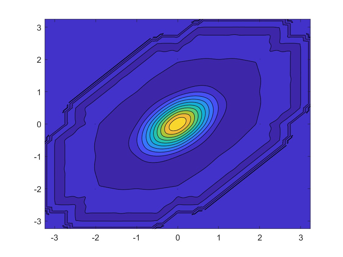
B Contour of $\phi$

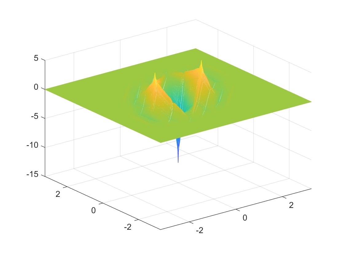
C $\frac{\partial^{2}\phi}{\partial x^{2}}\in C^{0}(\mathbb{R}^{2})$

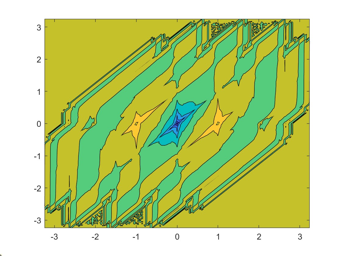
D Contour of $\frac{\partial^{2}\phi}{\partial x^{2}}$

E $\phi\in\mathscr{C}^{2}(\mathbb{R}^{2})$

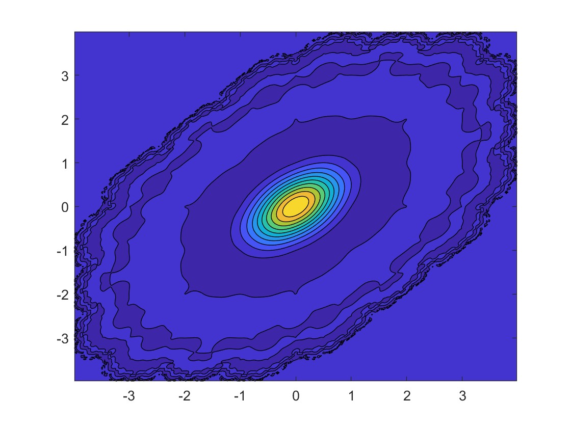
F Contour of $\phi$

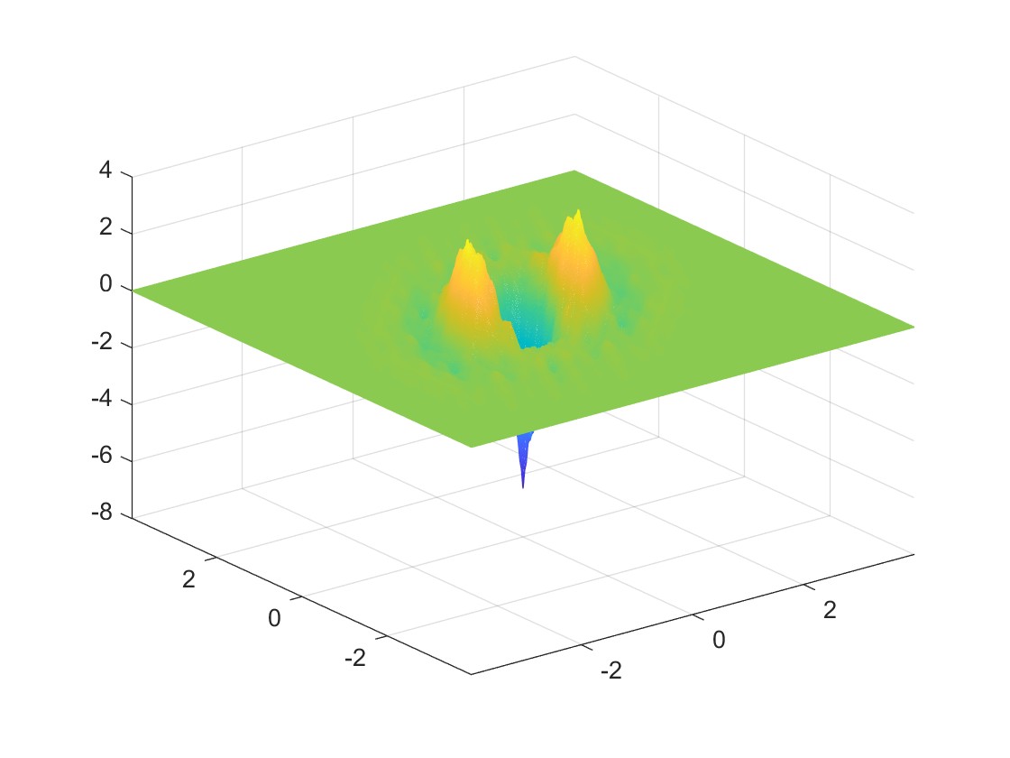
G $\frac{\partial^{2}\phi}{\partial x^{2}}\in C^{0}(\mathbb{R}^{2})$

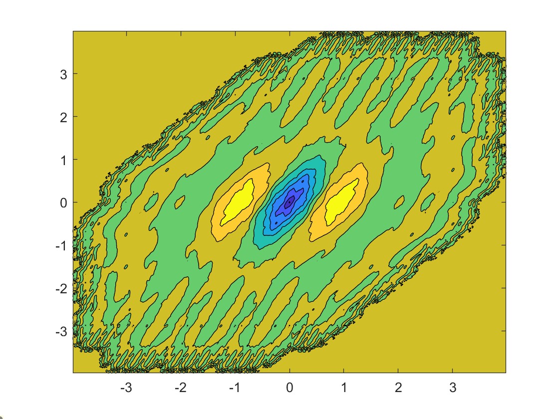
H Contour of $\frac{\partial^{2}\phi}{\partial x^{2}}$

Figure 4. The first row is for the first choice in Example 4: (A) is the graph of the interpolating $4I_{2}$-refinable function $\phi\in C^{2}(\mathbb{R}^{2})$ and (B) is its contour. (C) is the graph of the partial derivative $\frac{\partial^{2}\phi}{\partial x^{2}}\in C^{0}(\mathbb{R}^{2})$, and (D) is the contour of $\frac{\partial^{2}\phi}{\partial x^{2}}$. The second row is for the second choice in Example 4: (E) is the graph of the interpolating $4I_{2}$-refinable function $\phi\in C^{2}(\mathbb{R}^{2})$ and (F) is its contour. (G) is the graph of the partial derivative $\frac{\partial^{2}\phi}{\partial x^{2}}\in C^{0}(\mathbb{R}^{2})$, and (H) is the contour of $\frac{\partial^{2}\phi}{\partial x^{2}}$.

References

- [1] A. S. Cavaretta, W. Dahmen and C. A. Micchelli, Stationary subdivision. Mem. AMS Am. Math. Soc. 93 (1991), 453.
- [2] M. Charina and C. Conti, Polynomial reproduction of multivariate scalar subdivision schemes, J. Comput. Appl. Math. 240 (2013), 51–61.
- [3] C. Conti, L. Romani and J. Yoon, Approximation order and approximate sum rules in subdivision. J. Approx. Theory 207 (2016), 380–401.
- [4] C. K. Chui and Q. T. Jiang, Matrix-valued symmetric templates for interpolatory surface subdivisions. I. Regular vertices. Appl. Comput. Harmon. Anal. 19 (2005), 303–339.
- [5] C. K. Chui and Q. T. Jiang, Matrix-valued subdivision schemes for generating surfaces with extraordinary vertices. Comput. Aided Geom. Design 23 (2006), 419–438.
- [6] D. R. Chen, R. Q. Jia and S. D. Riemenschneider, Convergence of vector subdivision schemes in Sobolev spaces. Appl. Comput. Harmon. Anal. 12 (2002), 128–149.
- [7] C. Conti and S. López-Ureña, Non-oscillatory butterfly-type interpolation on triangular meshes, J. Comput. Appl. Math. 420 (2023), Paper No. 114788, 24 pp.
- [8] G. Deslauriers and S. Dubuc, Symmetric iterative interpolation processes. Constr. Approx. 5 (1989), 49–68.
- [9] C. Diao and B. Han, Quasi-tight framelets with high vanishing moments derived from arbitrary refinable functions, Appl. Comput. Harmon. Anal., 49 (2020), 123–151.
- [10] S. Dubuc, B. Han, J.-L. Merrien and Q. Mo, Dyadic Hermite interpolation on a square mesh. Comput. Aided Geom. Design 22 (2005), 727–752.
- [11] N. Dyn and D. Levin, Subdivision schemes in geometric modelling. Acta Numer. 11 (2002), 73–144.
- [12] N. Dyn, D. Levin and J. A. Gregory, A -point interpolatory subdivision scheme for curve design. Comput. Aided Geom. Design 4 (1987), 257–268.
- [13] N. Dyn, D. Levin and J. A. Gregory, A butterfly subdivision scheme for surface interpolation with tension control. ACM Transactions on Graphics 9 (1990), 160–169
- [14] L. Fang, B. Han and Y. Shen, Quasi-interpolating bivariate dual -subdivision using 1D stencils. Comput. Aided Geom. Design 98 (2022), Paper No. 102139, 18 pp.
- [15] L. Gemignani, L. Romani and A. Viscardi, Bezout-like polynomial equations associated with dual univariate interpolating subdivision schemes. Adv. Comput. Math. 48 (2022), no. 1, Paper No. 4, 27 pp.
- [16] B. Han, Subdivision schemes, biorthogonal wavelets and image compression. Ph.D. thesis at the University of Alberta. (1998) 138 pp.
- [17] B. Han, Analysis and construction of optimal multivariate biorthogonal wavelets with compact support. SIAM J. Math. Anal. 31 (2000), 274–304. Appl. Comput. Harmon. Anal. 13 (2002), 89–102.
- [18] B. Han, Vector cascade algorithms and refinable function vectors in Sobolev spaces. J. Approx. Theory 124 (2003), 44–88.
- [19] B. Han, Computing the smoothness exponent of a symmetric multivariate refinable function. SIAM J. Matrix Anal. Appl. 24 (2003), 693–714.
- [20] B. Han, Framelets and wavelets: algorithms, analysis, and applications. Applied and Numerical Harmonic Analysis. Birkhäuser/Springer, Cham, 2017. xxxiii + 724 pp.
- [21] B. Han, Multivariate Generalized Hermite Subdivision Schemes. Constr. Approx. 58 (2023), 407–462.
- [22] B. Han, Interpolating refinable functions and -step interpolatory subdivision schemes, Adv. Comput. Math., 50 (2024), article number 98
- [23] B. Han and R. Q. Jia, Multivariate refinement equations and convergence of subdivision schemes. SIAM J. Math. Anal. 29 (1998), 1177–1199.
- [24] B. Han and R.-Q. Jia, Optimal interpolatory subdivision schemes in multidimensional spaces. SIAM J. Numer. Anal. 36 (1998), 105–124
- [25] B. Han and R. Q. Jia: Optimal -two-dimensional interpolatory ternary subdivision schemes with two-ring stencils. Math. Comp. 75 (2006), 1287–1308.
- [26] B. Han and R. Lu: Compactly supported quasi-tight multiframelets with high balancing orders and compact framelet transform. Appl. Comput. Harmon. Anal. 51 , 295–332 (2021).
- [27] B. Han and M. Michelle, Wavelets on intervals derived from arbitrary compactly supported biorthogonal multiwavelets. Appl. Comput. Harmon. Anal. 53 (2021), 270–331.
- [28] B. Han, T. Yu and Y. Xue, Noninterpolatory Hermite subdivision schemes. Math. Comp. 74 (2005), 1345–1367.
- [29] B. Jeong, H. Yang and J. Yoon, Construction of a modified butterfly subdivision scheme with -smoothness and fourth-order accuracy, Appl. Math. Lett. 154 (2024), Paper No. 109087, 7 pp.
- [30] R. Q. Jia and Q. T. Jiang, Spectral analysis of the transition operator and its applications to smoothness analysis of wavelets. SIAM J. Matrix Anal. & Appl. 24 (2003), 1071–1109.
- [31] Q. T. Jiang, B. Li and W. Zhu, Interpolatory quad/triangle subdivision schemes for surface design. Comput. Aided Geom. Design 26 (2009),904–922.
- [32] Q. T. Jiang and P. Oswald, Triangular -subdivision schemes: the regular case. J. Comp. Appl. Math. 156 (2003), 47–75.
- [33] R. Lu, Interpolatory quincunx quasi-tight and tight framelets. Ann. Funct. Anal. 15 (2024), 85.
- [34] J-L. Merrien and T. Sauer, Generalized Taylor operators and polynomial chains for Hermite subdivision schemes. Numer. Math. 142 (2019), 167–203.
- [35] H. M. Möller and T. Sauer, Multivariate refinable functions of high approximation order via quotient ideals of Laurent polynomials. Adv. Comput. Math. 20 (2004), 205–228.
- [36] P. Novara, L. Romani and J. Yoon, Improving smoothness and accuracy of modified butterfly subdivision scheme. Appl. Math. Comput. 272 (2016), 64–79.
- [37] T. Sauer, Multivariate refinable functions, differences and ideals–a simple tutorial. J. Comput. Appl. Math. 221 (2008), 447–459.
- [38] T. Sauer, Polynomial interpolation, ideals and approximation order of multivariate refinable functions. Proc. Amer. Math. Soc. 130 (2002), 3335–3347.
- [39] S. D. Riemenschneider and Z. W. Shen: Multidimensional interpolatory subdivision schemes. SIAM J. Numer. Anal. 34 (1997), 2357–2381.