Suitability Analysis of Ground Motion Prediction Equations for Western and Central Himalayas and Indo-Gangetic Plains

Abstract

Ground motion prediction equations (GMPEs) play a key role in seismic hazard assessment (SHA). Considering the seismo-tectonic, geophysical and geotectonic characteristics of a target region, all the GMPEs may not be suitable in predicting the observed ground motion effectively. With a fairly large number of published GMPEs, the selection and ranking of suitable GMPEs for the design of logic trees in SHA for a particular target region has become a necessity of late. This paper presents a detailed quantitative evaluation of performance of 16 GMPEs against recorded ground motion data in two target regions, characterized by distinct seismo-tectonic, geophysical and geotectonical nature. The data set comprises of 465 three-component spectral accelerograms corresponding to 122 earthquake events. The suitability of a GMPE is tested by two widely accepted data-driven statistical methods, namely, likelihood (LH) and log-likelihood (LLH) method. Different suites of GMPEs are shown suitable for different periods of interest. The results will be useful to scientists and engineers for microzonation and estimation of seismic design parameters for the design of earthquake-resistant structures in these regions.

1 Introduction

Seismic hazard assessment (SHA) or more specifically probabilistic seismic hazard assessment (PSHA) is the most important tool for design of earthquake resistant structures and seismic risk mitigation. The aim of PSHA is to estimate the annual probability of exceedance (PoE) of a ground motion parameter of interest for a particular target region which exhibits a characteristic attenuation of that ground motion parameter as a function of a number of independent variables. For engineering purposes, the ground motion parameters are generally expressed quantitatively in terms of peak ground acceleration (PGA) and 5$\%$ damped pseudo-spectral acceleration (PSA) at different time periods of engineering interest. The PGA and PSA are predicted from ground motion prediction equations (GMPEs) which are model fitting to represent the functional form of recorded data by regression analysis. The GMPEs estimate PGA or PSA as a function of independent variables such as earthquake magnitude, source-to-site distance and site amplification effects along with various other parameters such as fault type, hanging wall effect etc. Therefore, for a reliable and realistic estimate of ground motion parameters, the selection of appropriate GMPEs is of extreme importance. The selected GMPEs should represent the ground motion of the region under study in a realistic manner. It needs to be mentioned here that the prediction of ground motion parameters from GMPEs depends on various parameters, all of which are not precisely known and therefore cannot be taken into account with confidence. Therefore, certain degree of subjectivity is always associated with the implementation of GMPEs. These uncertainties are classified into two types: (i) aleatory uncertainty which is taken care of by the residual scatter, generally denoted by $\sigma$, of the GMPEs and (ii) epistemic uncertainty which arises due to insufficient knowledge. For example, a number of GMPEs may be proposed for a particular target region and there is no a priori justification that one is more acceptable than the others (which indicates the lack of knowledge) (Cotton et al., 2006). This epistemic uncertainty is taken care of by involving multiple GMPEs in a logic tree framework (Kulkarni et al., 1984; Bommer and Scherbaum, 2008). Each branch of the logic tree corresponds to a different GMPE and proper weights should be assigned to each branch (i. e. each GMPE) in the PSHA calculations to arrive at the final value of the ground motion parameters. In other words, data-driven selection and ranking of the GMPEs for performing SHA in a target region is necessary.

Different quantitative data-driven methods (Scherbaum et al., 2004, 2009; Kale and Akkar, 2013; Kowsari et al., 2019) have been proposed so far to guide the selection of appropriate GMPEs. Among the existing methods, Scherbaum et al. (2004) first proposed a data-driven method, based on exceedance probabilities, to quantify the suitability of a candidate GMPE against recorded data. The method, now widely known as likelihood (LH) method, although not free from certain subjectivities, is based on sound mathematical background. Later Scherbaum et al. (2009) proposed another data-driven quantitative method, based on information theory, to decide the appropriateness of a candidate GMPE and thereafter assigning the weights to the branch of the logic tree. This method, now widely known as log-likelihood (LLH) method, does not depend on ad hoc assumptions (Delavaud et al., 2009) and therefore overcomes the limitations of the LH method.

The suitability of GMPEs in different regions has earlier been tested (Hintersberger et al., 2007; Stafford et al., 2008; Arango et al., 2012; Beauval et al., 2012; Bykova, 2016; Sinha and Selvan, 2022) using different methods. Here the suitability of various GMPEs are examined by performing a thorough quantitative assessment in a systematic way to target regions which exhibit complex seismo-tectonic setup and are characterized by distinct geophysical and geotechnical properties. A detailed systematic study of applicability of the GMPEs for the said target regions has not been carried out earlier to the best of our knowledge.

The following section gives a brief description of target regions, followed by a description of data sets used in the study and then list of GMPEs considered for the present study. Section 5 elucidates the data-driven methods. The next section presents the results in each target region with detailed discussions of the results. Section 7 draws the conclusions.

2 Target Regions with their Seismotectonic Framework

Knowledge of seismotectonic characteristics of a region is important to ascertain the seismic potential of the region and to evaluate the probable ground motion that it can generate. The two target regions, considered for the present study, constitute intricate and complex seismotectonic environment and exhibit distinct geological characteristics. These two target regions, namely, (i) Western and Central Himalayas and (ii) Indo-Gangetic Plains are shown in Fig. 1. The epicenters of past earthquakes, taken from the reviewed International Seismological Centre (ISC) bulletin, UK (http://www.isc.ac.uk/iscbulletin/search/bulletin/), National Earthquake Information Centre (NEIC), (https://earthquake.usgs.gov/earthquakes/search/), USGS and India Meteorological Department (IMD), New Delhi and various tectonic features taken from (Dasgupta et al., 2000) are also plotted in Fig. 1. Gupta (2006) has extensively analysed the seismotectonic characteristics of the Himalayas and northeast India and brought out a wide picture of seismic sources in these regions.

Kayal et al. (2022), after analysing the seismic cross sections and focal plane solutions of the region, suggested that the source process of the entire Himalayas have heterogeneous seismotectonic patterns.

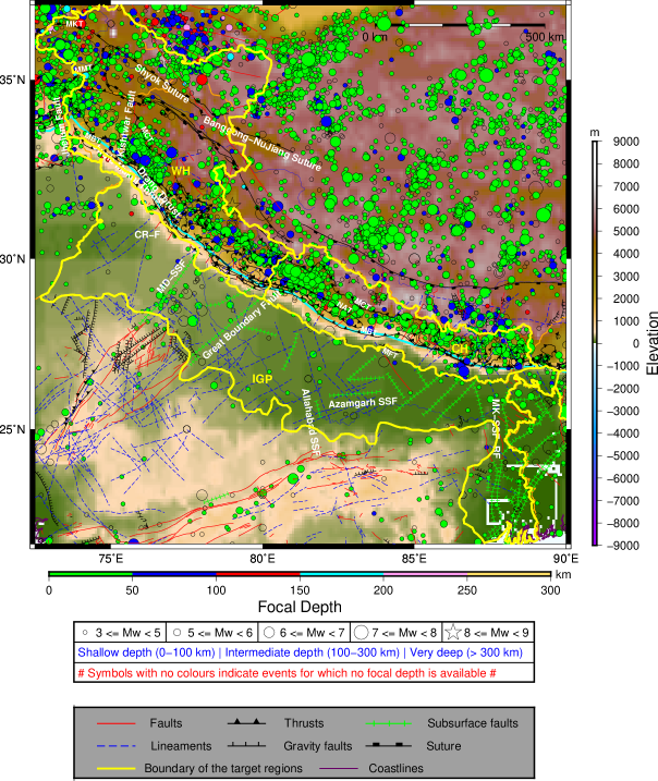
Figure 1: Map showing the target regions with various tectonic features (Dasgupta et al., 2000) and the epicenters of past earthquakes superimposed therein. The international boundaries and coastlines are produced from the Generic Mapping Tools (GMT) database. WH stands for western Himalaya, CH stands for central Himalaya and IGP stands for Indo-Gangetic Plains.

2.1 The Western and Central Himalayas

The western and central Himalayas within the framework of the Himalayan arc tectonic belt is dominated by seismically active thrust faults which produce large magnitude earthquakes due to the interaction between Indian and Eurasian continental plates. The geology of the entire region is possessed by various rock formations such as schist, quartzite, slates, phyllites, gneisses and granites. The predominant thrust faults include Main Central Thrust (MCT), Main Boundary Thrust (MBT) and Main Frontal Thrust (MFT) along with many subsidiary thrusts. The decollement surface which is the plane of detachment between Indian and Eurasian plates is considered to be responsible for few of the great earthquakes (1991 Uttarkashi and the 1999 Chamoli earthquakes having magnitude $>$ 6.0) that occurred north of MBT in this region (Kayal, 2010). The 2015 Nepal earthquake of $M_{w}$ 7.8 was caused by reverse faulting at the down-dip portion of the Main Himalayan Thrust (MHT) (Kumar et al., 2016). Apart from the thrust faults, many transverse and oblique faults also occupy this region which cause the long extends of MBT and MCT break into fragments (Gupta, 2006). Kayal (2014) reports few great earthquakes caused by strike-slip faulting in this region (1988 Bihar/Nepal foothill Himalaya and 2011 Sikkim Himalaya earthquakes having magnitude $>$ 6.0). Nayak and Sitharam (2019) reported a maximum magnitude 7.7 for western Himalaya and 8.0 for central Himalaya.

2.2 The Indo-Gangetic Plains

The Indo-Gangetic plains are large floodplains of the Indus, Ganga, Yamuna and the Brahmaputra river systems (B. Naresh and Mishra, 2021). They run parallel to the Himalaya mountains, from Jammu and Kashmir and Khyber Pakhtunkhwa in the west to the western part of northeast India in the east. This region, even though characterised by moderate earthquakes, has high influence of seismic activities in the adjacent western and central Himalayas and shows widespread alluvial deposits which constitute considerable site amplifications. This region witnesses several subsurface faults (SSFs) including Azamgarh SSF and Allahabad SSF. The Indus basin is comprised of Chandhigar Ropar fault (a neotectonic fault), North-Delhi fold belt and Mahendragarh and Dehradun SSFs. The Ganga basin contributes many dip slip, oblique and strike slip faults which cross transverse to the Himalayan Frontal thrust zone. The quaternary alluvial deposits in the Bengal basin cover the state of West Bengal. Maldah-Kishanganj fault, Rajmahal fault and many neotectonic faults are present in the Bengal basin with moderate seismic activities (Dasgupta et al., 2000). Anbazhagan et al. (2015) reported a maximum magnitude of 7.0 by considering the regional rupture characteristics for Patna region which lies in Indo-Gangetic plains while a maximum magnitude of 6.6 was reported by Nayak and Sitharam (2019) for Indo-Gangetic plains.

3 Ground-Motion Data Set

A total of 122 earthquakes from 163 recording Stations have been considered for for performing the efficacy test of the GMPEs for the said target regions. These earthquakes correspond to a total of 465 three-component ground-motion accelerograms (i.e, $465\times 2=930$ horizontal accelerograms) which are used for examining the suitability of GMPEs in the said target regions. Out of this 465 records, 356 records ($356\times 2=712$ horizontal accelerograms) from 96 recording Stations are from northwest and central Himalayas while 109 records ($109\times 2=218$ horizontal accelerograms) from 53 recording Stations are from Indo-Gangetic plains. It is observed that western side of IGP has good distribution of recording stations compared to the eastern side of IGP. However, out of 53 stations in IGP, Delhi and its surrounding area have 32 stations while the remaining 21 stations are distributed in the rest of IGP.

For northwest and central Himalaya region, the magnitude and the distance (epicentral) range of the earthquake events are 3.0 - 7.8 and 2 - 340 km respectively and the same for Indo-Gangetic plains are 3.0 - 6.8 and 1 - 366 km respectively. The locations of the earthquake epicenters and the recording stations are shown in Fig. 2.

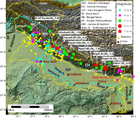
Figure 2: Map showing the locations of recording stations and earthquake epicenters of the recorded data used in the study. The boundary of the two target regions are marked in yellow color. The DEM data are taken from GLOBE model of NOAA.

The region under study has witnessed several devastating earthquakes in the past. Some significant earthquakes whose acclerograms are used in the present analysis are listed in Table 1.

Table 1: Some significant earthquakes in the region of study

Name of Date Lat Lon Focal Depth Magnitude Fault Earthquake (dd-mm-yy) ($\degree N$) ($\degree E$) (km) ($M_{W}$) Type Chamoli-Mainshock 28-03-1999 30.512 79.403 15.0 6.6 Reverse Chamoli-Aftershock 28-03-1999 30.315 79.380 10.0 5.4 Reverse Chamoli-Aftershock 30-03-1999 30.376 79.330 10.0 5.3 Reverse Chamoli-Aftershock 06-04-1999 30.414 79.320 10.0 5.1 Reverse Chamoli-Aftershock 07-04-1999 30.250 79.320 10.0 5.0 Reverse Chamoli-Aftershock 07-04-1999 30.260 79.310 10.0 5.2 Reverse JK-HP-Border 01-05-2013 33.100 75.800 15.0 5.8 Strike-slip Nepal-India Border 04-04-2011 29.600 80.800 10.0 5.7 Strike-slip India(Sikkim)-Nepal 18-09-2011 27.600 88.200 10.0 6.8 Strike-slip India(Sikkim)-Nepal (AS) 18-09-2011 27.600 88.500 16.0 5.0 Strike-slip Uttarkashi 19-10-1991 30.780 78.774 10.0 7.0 Reverse Nepal-Mainshock 25-04-2015 28.150 84.710 15.0 7.8 Reverse Nepal-Aftershock 26-04-2015 27.760 85.770 10.0 5.3 Reverse Nepal-Aftershock 26-04-2015 27.780 86.000 17.3 6.7 Reverse Nepal-Aftershock 25-04-2015 27.910 85.650 10.0 5.7 Reverse Nepal-Aftershock 25-04-2015 28.190 84.870 14.6 7.2 Reverse Nepal-Aftershock 25-04-2015 27.805 84.874 10.0 5.8 Reverse Nepal-Aftershock 25-04-2015 27.640 85.500 10.0 5.5 Reverse Nepal-Aftershock 12-05-2015 27.840 86.080 15.0 7.3 Reverse Nepal-Aftershock 12-05-2015 27.620 86.170 15.0 6.8 Reverse

The distribution of dataset in terms of magnitude and distance is presented in Fig. 3.

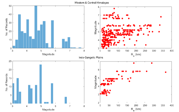
Figure 3: Distribution of earthquake records (left panel) and magnitude-distance scatter plot (right panel) of the data set used in the study.

The variation in the range of magnitude and distance in the data set make it appropriate to perform the efficacy test for different GMPEs. It is mentioned here that there are 21 aftershocks out of a total of 122 earthquakes and 41 earthquakes having magnitude lying in the range 3 $\leq$ $M_{w}$ $<$ 4 are there. Magnitudes below 4.0 are used to test the suitability of GMPEs as NGA-West2 GMPEs are developed by considering earthquakes having magnitudes less than 4.0. Although magnitudes less than 4.0 should not contribute significantly to seismic hazard estimation, Slejko and Rebez (2002) reported that, in moderate seismicity region, the lower threshold value of magnitude can be taken as 3.0.

It is worth mentioning that the data set considered for the present study was mostly not used by the developers of the GMPEs and is an independent data set. The ground-motion data set, used for the present study has been downloaded from PESMOS (https://pesmos.org). In addition, the PESMOS data have been supplemented by $53$ three-component ground-motion accelerograms (a total of $53\times 2=106$ horizontal accelerograms) from $21$ earthquakes of different hypo-central depths and these $53$ records have been downloaded from Center for Engineering Strong Motion Data (https://www.strongmotioncenter.org). The ground motion data set downloaded from the above sources are processed only (baseline corrected and low pass filtered). The processed downloaded data have been compiled in a consistent manner to tabulate magnitude, source-to-site distance metrics, local site conditions and PGA. The 5$\%$ damped PSA at different time periods have been computed from the processed acceleration time histories using standard computer programs.

It is added here that the site characteristics of all the recording stations were provided in the data set downloaded. While computing the PGA or PSA (at different time periods), the same site conditions were used to avoid any bias in the selection of suitable GMPEs. The set of suitable GMPEs, thus selected, may be used for computation of PGA or PSA (at different time periods) at any site inside a target region. The site condition of that particular site will then be an input parameter in the selected GMPEs. The details of the recording stations are given in the Supplementary Material.

4 List of GMPEs Considered

There have been considerable advances in the development of GMPEs with the increase of seismic networks since 2000. A very good account of the empirical GMPEs existing throughout the world for the period 1964-2021 is well documented in the report by Douglas (2022). Following the minimum criteria proposed by Cotton et al. (2006) and Bommer et al. (2010), 16 GMPEs for crustal earthquakes have been primarily selected for performing the efficacy test and ranking of the GMPEs. All the GMPEs are mostly recent GMPEs, robust and adequately constrained. Out of the 16 GMPEs, 12 GMPEs have been developed from world wide data and the remaining are developed for other regions including one for Himalayan region. All the GMPEs with their range of applicability is listed in Table 2.

It needs to be mentioned here that limited seismic network and paucity of ground motion data in India imposes a limitation for developing robust GMPEs empirically, exclusively for the regions under study. It is also added here that the observation of Cotton et al. (2006) that a GMPE, developed for a region which does not conform tectonically to the region under study should be excluded, cannot possibly be true as the selection or exclusion of a GMPE can never be based on geographical criteria (Bykova, 2016; Bommer et al., 2010). Several studies show that there is no solid evidence of regional differences in ground motions in tectonically comparable regions, at least in the range of moderate to high magnitude earthquakes (Stafford et al., 2008; Douglas, 2007), with few exceptions in active regions (Strasser et al., 2009) for high-frequency response spectra. Rather, this criterion should be interpreted as to exclude the GMPEs, developed for subduction earthquakes, in PSHA calculations for shallow crustal earthquakes and vice versa, or for example, the GMPEs made for volcanic areas should not be used in regions which does not exhibit volcanic activities. Therefore, after preliminary analysis, the GMPEs, listed in Table 2, have been considered for the target regions.

It is mentioned here that few region-specific GMPEs (Sharma et al., 2009; Nath et al., 2012; Singh et al., 2017; Gupta and Trifunac, 2018; Nh and Kumar, 2020) are not shown in the present analysis for practical limitations with these GMPEs in the context of the present analysis. For example, Sharma et al. (2009) and Gupta and Trifunac (2018) considered time periods starting from 0.04 s. Now, the PSA at 0.04 sec cannot be treated equivalent to PGA. On the other hand, Nath et al. (2012) proposed their GMPE for 8 periods (including PGV) only ranging from PGA to 4.0 s with wide intervals. The PSA at many periods in between are not available, which makes it difficult to arrive at a conclusive result. The GMPE, proposed by Singh et al. (2017) considered only one main shock (Nepal earthquake) and five aftershocks. The database is fairly small for developing a robust GMPE. This GMPE did neither consider the fault type nor the soil response term. Moreover, 0.2 s time period, which is a crucial one for this study, is not there in this GMPE. The GMPE, proposed by Nh and Kumar (2020), considered a small database (only 15 earthquakes), of which 4 events are above 6.0 $M_{w}$. Due to these practical limitations, these regional GMPEs were not found suitable for testing the LH and the LLH methods as the LH ranks and LLH scores are expected to be inconsistent compared with the other GMPEs considered. It is pointed out that the three most important criteria for primarily rejecting a GMPE for consideration, as per Cotton et al. (2006), are (i) The underlying dataset for developing the GMPE is insufficient, (ii) The frequency range of the model is not appropriate for engineering application and (iii) The model has an inappropriate functional form. The present analysis is focussed on testing two well established methods for selection of best suitable GMPEs in two target regions and GMPEs that allow to arrive at a conclusive result are considered.

Table 2: GMPEs considered in this study with their range of applicability

GMPEs with abbreviations Magnitude Distance $V_{s30}$ Periods Region and references ($M_{W}$) range range (km) range (m/s) (s) KAN06 (Kanno et al. (2006)) 5.5 - 8.2 $<$ 450 150 - 1500 0.0 - 5.0 Japan ZHAO06 (Zhao et al. (2006)) 5 - 7.5 0 - 300 4 site classes 0.0 - 5.0 Japan AS08 (Abrahamson and Silva (2008)) 5 - 8.5 $<$ 200 $>$ 180 0.0 - 10 Worldwide BA08 (Boore and Atkinson (2008)) 5 - 8.0 0 - 200 180 - 1300 0.0 - 10 Worldwide CB08 (Campbell and Bozorgnia (2008)) 4 - 8.5 0 - 200 150 - 1500 0.0 - 10 Worldwide CY08 (Chiou and Youngs (2008)) 4 - 8.5 0 - 200 150 -1500 0.0 - 10 Worldwide IDR08 (Idriss (2008)) 4.5 - 8 0 - 200 $>$ 450 0.0 - 10 World wide AKBO10 (Akkar and Bommer (2010)) 5 - 7.6 $<$ 100 3 site classes 0 - 3.0 EMM ASK14 (Abrahamson et al. (2014)) 3 - 8.5 0 - 300 180 - 1500 0.0 - 10 World wide BSSA14 (Boore et al. (2014)) 3.0 - 8.5 (SS, RV) 3.3 - 7.0 (NM) 0 - 400 150 - 1500 0.0 - 10 World wide CB14 (Campbell and Bozorgnia (2014)) 3.3 - 8.5 (SS) 3.3 - 8.0 (RV) 3.3 - 7.0 (NM) 0 - 300 150 - 1500 0.01 - 10 World wide CY14 (Chiou and Youngs (2014)) 3.5 - 8.5 (SS) 3.5 - 8.0 (RV, NM) 0 - 300 180 - 1500 0.0 - 10 World wide IDR14 (Idriss (2014)) 5 - 8.0 0 - 150 450 - 2000 0.0 - 10 World wide GK15 (Graizer and Kalkan (2016)) 5.0 - 8.0 0 - 250 200 - 1300 0.01 - 5.0 World wide ZHAO16 (Zhao et al. (2016)) 5 - 7.5 0 - 300 4 site classes 0.0 - 5.0 Worldwide BJAN19 (Bajaj and Anbazhagan (2019)) 4 - 9.0 10 - 750 NA 0.0 - 10 Himalaya * SS = Strike slip, RV = Reverse, NM = Normal; EMM = Europe, Mediterranean and Middle East

5 Data-driven methods

In this section, we will discuss two methods, namely the LH and the LLH method, to judge the goodness-of-fit measures between observed ground motion data for a target region and a candidate GMPE. There are several methods for evaluating the goodness-of-fit measures (Scherbaum et al., 2004, 2009; Kale and Akkar, 2013; Kowsari et al., 2019). LH method is a transparent one which is based on the concept of likelihood (Edwards, 1992) and is particularly useful in examining the match or mismatch of recorded data to a GMPE for a target region. The level of agreement between the observations and the predictions in LH method is quantitatively expressed in terms of mean, median and standard deviation of the normalized residual and the median values of the LH parameter as well. Under the assumption that a ground motion parameter (say $y$) obeys log-normal distribution (i.e, $\ln y$ is normally distributed), the normalized residual is expressed as

$$Z=\frac{\ln({y})_{\tt obs}-\ln({y})_{\tt predicted}}{\sigma_{\tt T}}$$ (1)

where $({y})_{\tt obs}$ and $({y})_{\tt predicted}$ are the observed and the predicted ground motions and $\sigma_{\tt T}$ is the total standard deviation of the GMPE used. So normalized residual ($Z$) represents the distance of the data from the logarithmic mean measured in units of $\sigma_{\tt T}$. The LH parameter is calculated as

$$LH(|Z|)=Erf(\frac{|Z|}{\sqrt{2}},\infty)=\frac{2}{\sqrt{2\pi}}\int_{|Z|}^{\infty}exp\left(\frac{-Z^{2}}{2}\right)dZ$$ (2)

where $Erf$ is the error function. The median of $LH$ plays an important role in quantifying the suitability of a GMPE. If the chosen GMPE matches the observed data well in terms of both the mean and the standard deviation, then the $LH$ values are evenly distributed between $0$ and $1$ and the median of $LH$ is $\sim 0.5$. In case the GMPE is unbiased in terms of mean but the standard deviation of the observed data is either smaller or greater than the standard deviation of the GMPE, the distribution of $LH$ becomes asymmetric and the median value of $LH$ is either $>0.5$ or $<0.5$. The more the standard deviation of the observed data and the shift of the mean value, the less is the median of the $LH$ distribution. These properties make the $LH$ method a good one to check the suitability of a GMPE against recorded data. Although, it is not only the median value of the $LH$ distribution but also the mean, median and the standard deviation of the normalized residual that decide the goodness-of-fit measures of $LH$ method. Depending on these measures, Scherbaum et al. (2004) proposed a classification scheme for ranking of GMPEs to evaluate the performance of GMPEs against recorded ground motion data. The four goodness-of-fit measures for deciding the rank of a GMPE are listed in Table 3.

Table 3: Values of goodness-of-fit measures for deciding the rank of a GMPE

$\mid\text{Mean}\ \textit{Z}\mid$ $\mid\text{Median}\ \textit{Z}\mid$ Std $Z$ Med. $LH$ Rank $<$ 0.25 $<$ 0.25 $<$ 1.125 $>$ 0.4 A (high capability) $<$ 0.50 $<$ 0.50 $<$ 1.250 $>$ 0.3 B (medium capability) $<$ 0.75 $<$ 0.75 $<$ 1.500 $>$ 0.2 C (low capability) All other combinations of goodness-of-fit measures D (unacceptable capability)

However, the $LH$ method is dependent on the sample size, i.e, the total number of recorded grounded motion data and despite its statistical relevance, the $LH$ method is not completely free from certain subjectivities. The subjectivities lie in the threshold values of the goodness-of-fit measures and in the definition of ranks. To overcome these limitations, Scherbaum et al. (2009) proposed another goodness-of- fit method, the so-called LLH method, which does not depend on ad hoc assumptions.

LLH method is based on the concepts of information theory. The fundamental aim of LLH method is to measure the Kullback-Leibler (KL) distance between two models - a model that represents reality (here the ground motion data) and a candidate ground motion model (here a GMPE). If two models $f$ and $g$ be described by two probability density functions $f(x)$ and $g(x)$, the KL distance between the two models is expressed as (Scherbaum et al., 2009)

$$D(f,g)=E_{f}[\log_{2}(f)]-E_{f}[\log_{2}(g)]$$ (3)

where $E_{f}$ is the statistical expectation of the log-likelihood of the model function with respect to $f$. $D(f,g)$ is interpreted as the relative entropy between $f$ and $g$ (Cover and Thomas, 2006) and represents the amount of information loss if model $f$ is replaced by model $g$. The negative value of the statistical expectation of the log-likelihood function indicate a natural distance measure (Scherbaum et al., 2009). For comparison of models, the relative KL distance is of only interest as the statistical expectation of the log-likelihood of $f$ with respect to $f$ cancels out as a constant term (Scherbaum et al., 2009). Therefore, to specify a ranking criterion, the log-likelihood score may be defined as

$$LLH=-\frac{1}{N}\sum_{n=i}^{N}\log_{2}(g(x_{i}))$$ (4)

where $N$ is the total number of observations. This LLH score is termed as average sample log-likelihood. The Eqn. 4 for LLH score is more explicitly written as

$$LLH=-\frac{1}{N}\sum_{n=i}^{N}\log_{2}\left[\frac{1}{\sigma_{i}\sqrt{2\pi}}\exp\left\{-\frac{1}{2}\left(\frac{y_{i}-\mu_{i}}{\sigma_{i}}\right)^{2}\right\}\right]$$ (5)

where $y_{i}$ is the observed ground motion value and $\mu_{i}$ and $\sigma_{i}$ are the mean and the standard deviation of the GMPE being considered. A lower LLH score implies a better performance of a GMPE for a target region. In LLH method, only one measure, i.e, LLH score, which basically indicates the average loss of information when the model representing reality is replaced by a candidate GMPE, is required to examine the suitability of a GMPE. On the contrary, a combination of four measures is required to decide the ranking criteria in LH method, as discussed earlier. Therefore the LLH method may be treated as a better one.

6 Results and discussion

In this section, the results obtained from our analysis are presented. The analyses are carried out in two target regions and the performance of 16 GMPEs is evaluated at 20 periods using the two data-driven methods, discussed in the previous section.

6.1 Results for Western and Central Himalaya

Table LABEL:rewch presents the various goodness-of-fit measures at 9 different periods for all the GMPEs considered. The values for the period $0.01$ s may be treated as the values for PGA. PSA at $0.2$ s and $1.0$ s are frequently used as corner spectral periods to construct design spectrum for structural design.

Table 4: Various goodness-of-fit measures for all the GMPEs considered in western and central Himalayas

GMPEs	Goodness-of-fit					Periods (s)
Considered	measures	0.01	0.02	0.05	0.10	0.20	0.30	0.50	1.00	2.00
KAN06	Mean $Z$	0.25	0.29	0.29	0.29	0.18	-0.10	-0.40	-0.61	-0.48
	Median $Z$	0.26	0.29	0.28	0.23	0.20	-0.08	-0.47	-0.59	-0.64
	Std $Z$	1.09	1.09	1.16	1.08	1.16	1.17	1.07	1.04	1.24
	Med. $LH$	0.47	0.48	0.44	0.45	0.40	0.38	0.42	0.43	0.34
	Rank	B	B	B	B	B	B	B	C	C
	$LLH$ Score	2.00	2.02	2.13	2.11	2.21	2.17	2.18	2.29	2.44
ZHAO06	Mean $Z$	-0.08	-0.23	-0.06	0.03	-0.01	-0.30	-0.75	-0.92	-0.86
	Median $Z$	-0.07	-0.21	-0.05	0.01	0.03	-0.29	-0.79	-0.92	-0.98
	Std $Z$	1.23	1.21	1.22	1.10	1.27	1.34	1.30	1.26	1.37
	Med. $LH$	0.41	0.42	0.47	0.44	0.42	0.31	0.29	0.29	0.22
	Rank	B	B	B	A	C	C	D	D	D
	$LLH$ Score	1.95	2.00	2.03	1.97	2.18	2.31	2.56	2.71	2.88
AS08	Mean $Z$	-0.29	-0.26	-0.08	0.05	-0.25	-0.58	-0.93	-1.01	-0.68
	Median $Z$	-0.31	-0.29	-0.14	-0.04	-0.21	-0.56	-0.92	-0.98	-0.84
	Std $Z$	1.48	1.48	1.42	1.44	1.54	1.47	1.39	1.50	1.82
	Med. $LH$	0.33	0.32	0.41	0.33	0.32	0.26	0.24	0.23	0.20
	Rank	C	C	C	C	D	C	D	D	D
	$LLH$ Score	2.45	2.43	2.41	2.49	2.73	2.73	2.91	3.19	3.52
BA08	Mean $Z$	0.16	0.16	0.40	0.37	-0.03	-0.48	-1.07	-1.02	-0.24
	Median $Z$	0.15	0.12	0.33	0.39	0.06	-0.45	-1.03	-1.05	-0.81
	Std $Z$	1.75	1.75	1.79	1.65	1.65	1.57	1.57	1.64	2.23
	Med. $LH$	0.27	0.29	0.31	0.27	0.31	0.25	0.19	0.17	0.13
	Rank	D	D	D	D	D	D	D	D	D
	$LLH$ Score	2.73	2.72	2.97	2.67	2.54	2.55	3.22	3.40	4.42
CB08	Mean $Z$	-0.78	-0.75	-0.51	-0.25	-0.68	-1.08	-1.51	-1.07	-0.06
	Median $Z$	-0.75	-0.74	-0.49	-0.26	-0.58	-1.05	-1.51	-1.07	-0.50
	Std $Z$	1.66	1.66	1.63	1.51	1.67	1.73	1.70	1.67	2.16
	Med. $LH$	0.23	0.24	0.31	0.30	0.29	0.17	0.09	0.18	0.18
	Rank	D	D	D	D	D	D	D	D	D
	$LLH$ Score	2.83	2.78	2.62	2.29	2.91	3.55	4.28	3.48	4.04
CY08	Mean $Z$	0.55	0.56	0.64	0.93	0.75	0.47	0.07	-0.28	0.14
	Median $Z$	0.57	0.56	0.60	0.81	0.82	0.58	0.07	-0.43	-0.55
	Std $Z$	1.70	1.71	1.74	1.72	1.68	1.58	1.57	1.78	2.45
	Med. $LH$	0.28	0.26	0.30	0.21	0.24	0.28	0.31	0.21	0.16
	Rank	D	D	D	D	D	D	D	D	D
	$LLH$ Score	3.05	3.08	3.30	3.60	3.28	2.81	2.59	3.14	5.17
IDR08	Mean $Z$	-0.22	-0.18	-0.04	0.36	0.01	-0.44	-0.91	-1.18	-0.86
	Median $Z$	-0.14	-0.11	-0.03	0.36	0.13	-0.34	-0.95	-1.21	-1.02
	Std $Z$	1.41	1.41	1.40	1.30	1.41	1.39	1.30	1.21	1.25
	Med. $LH$	0.34	0.33	0.43	0.36	0.34	0.32	0.26	0.21	0.23
	Rank	C	C	C	C	C	C	D	D	D
	$LLH$ Score	2.30	2.27	2.23	2.21	2.39	2.52	2.86	3.16	2.82
AKBO10	Mean $Z$	0.38	0.28	0.59	0.51	0.01	-0.18	-0.23	0.16	0.43
	Median $Z$	0.42	0.33	0.60	0.54	0.08	-0.10	-0.26	-0.10	-0.11
	Std $Z$	1.54	1.56	1.64	1.51	1.44	1.40	1.38	2.03	2.46
	Med. $LH$	0.32	0.36	0.31	0.32	0.38	0.33	0.38	0.22	0.17
	Rank	D	D	D	D	C	C	C	D	D
	$LLH$ Score	2.51	2.53	2.95	2.60	2.30	2.25	2.33	3.89	5.41
ASK14	Mean $Z$	0.88	0.82	0.97	1.13	1.05	0.88	0.58	0.68	0.84
	Median $Z$	0.90	0.86	0.99	1.14	1.13	0.91	0.52	0.53	0.33
	Std $Z$	1.32	1.32	1.34	1.35	1.40	1.33	1.32	1.76	2.32
	Med. $LH$	0.28	0.30	0.25	0.20	0.21	0.25	0.31	0.26	0.25
	Rank	D	D	D	D	D	D	C	D	D
	$LLH$ Score	2.81	2.76	3.03	3.30	3.26	2.87	2.49	3.51	5.30
BSSA14	Mean $Z$	1.14	1.15	1.14	1.22	1.19	1.00	0.68	0.65	1.08
	Median $Z$	1.20	1.22	1.21	1.24	1.32	1.03	0.64	0.49	0.38
	Std $Z$	1.47	1.45	1.41	1.44	1.45	1.43	1.48	1.86	2.43
	Med. $LH$	0.16	0.16	0.19	0.17	0.14	0.19	0.30	0.29	0.32
	Rank	D	D	D	D	D	D	C	D	D
	$LLH$ Score	3.37	3.37	3.43	3.57	3.44	3.06	2.76	3.66	5.98
CB14	Mean $Z$	1.49	1.48	1.29	1.54	1.50	1.07	0.65	0.43	0.89
	Median $Z$	1.49	1.49	1.37	1.62	1.61	1.07	0.62	0.29	0.17
	Std $Z$	1.60	1.59	1.45	1.44	1.49	1.44	1.48	1.91	2.55
	Med. $LH$	0.12	0.12	0.14	0.09	0.10	0.20	0.30	0.25	0.29
	Rank	D	D	D	D	D	D	C	D	D
	$LLH$ Score	4.32	4.30	3.74	4.23	4.15	3.22	2.73	3.64	6.09
CY14	Mean $Z$	1.19	1.21	1.11	1.31	1.22	0.92	0.65	0.58	0.93
	Median $Z$	1.25	1.27	1.11	1.34	1.24	0.89	0.58	0.42	0.24
	Std $Z$	1.47	1.48	1.56	1.52	1.45	1.35	1.33	1.80	2.54
	Med. $LH$	0.17	0.17	0.18	0.14	0.15	0.23	0.32	0.30	0.30
	Rank	D	D	D	D	D	D	C	D	D
	$LLH$ Score	3.46	3.50	3.57	3.86	3.59	2.94	2.62	3.57	6.17
IDR14	Mean $Z$	-0.02	-0.02	0.14	0.34	0.20	-0.08	-0.37	-0.70	-0.41
	Median $Z$	0.00	-0.01	0.07	0.29	0.31	-0.09	-0.34	-0.64	-0.37
	Std $Z$	1.60	1.59	1.61	1.49	1.56	1.54	1.41	1.38	1.44
	Med. $LH$	0.24	0.24	0.28	0.28	0.24	0.24	0.33	0.30	0.40
	Rank	D	D	D	C	D	D	C	C	C
	$LLH$ Score	2.76	2.74	2.81	2.65	2.79	2.75	2.60	2.84	2.75
GK15	Mean $Z$	0.26	0.30	0.15	0.35	0.31	0.00	-0.62	-1.10	-0.92
	Median $Z$	0.10	0.13	-0.08	0.13	0.24	-0.04	-0.65	-1.23	-1.15
	Std $Z$	1.69	1.73	1.84	1.76	1.68	1.71	1.71	1.62	1.71
	Med. $LH$	0.33	0.33	0.32	0.34	0.34	0.24	0.17	0.15	0.17
	Rank	D	D	D	D	D	D	D	D	D
	$LLH$ Score	2.83	2.92	3.17	3.04	2.82	2.85	3.19	3.76	3.86
ZHAO16	Mean $Z$	-0.17	-0.17	-0.41	-0.27	0.23	0.32	0.25	0.09	0.01
	Median $Z$	-0.15	-0.16	-0.46	-0.32	0.28	0.38	0.28	0.14	-0.17
	Std $Z$	1.38	1.38	1.37	1.21	1.27	1.26	1.25	1.29	1.53
	Med. $LH$	0.37	0.37	0.41	0.42	0.38	0.39	0.40	0.38	0.31
	Rank	C	C	C	B	C	C	B	C	D
	$LLH$ Score	2.15	2.15	2.33	2.09	2.17	2.17	2.09	2.15	2.57
BJAN19	Mean $Z$	0.41	0.26	0.02	0.23	0.36	0.28	0.42	0.69	1.39
	Median $Z$	0.39	0.22	-0.12	0.07	0.33	0.31	0.42	0.51	0.89
	Std $Z$	1.16	1.12	1.15	1.11	1.18	1.25	1.39	1.87	2.50
	Med. $LH$	0.44	0.49	0.48	0.48	0.43	0.39	0.32	0.23	0.19
	Rank	B	B	B	A	B	B	C	D	D
	$LLH$ Score	2.12	2.08	2.17	2.14	2.15	2.17	2.46	3.79	6.79

It is evident from Table LABEL:rewch that each of the goodness-of-fit measures varies considerably with the periods for all the GMPEs and therefore the performance of GMPEs are period-dependent. It is also observed that the NGA-West1 GMPEs, except AS08 and IDR08, fall into ‘unacceptable category’ for all the $9$ periods in this target region. The AS08 and the IDR08 show ‘low capability’ at lower periods. The NGA-West2 GMPEs are not suitable too for most of the periods. However, ASK14 and IDR14 show better LLH scores than the other NGA-West2 GMPEs. It is interesting to note that the NGA-West1 GMPEs perform better than the NGA-West2 GMPEs in terms of LLH score, especially at lower periods, given the set of available data in this target region. As per the ranking criteria in LH method, KAN06 shows no ‘unacceptable category’ at any period. From our analysis, a combination of ZHAO06, KAN06, BJAN19 and ZHAO16 are seen to best perform at $0.01$ s and may be selected as a suitable combination for this period, compared to the other GMPEs, for populating the branches of the logic tree in PSHA. Since LLH method is considered better than LH method (as explained earlier), ZHAO06 may be treated as the most suitable GMPE for periods $\leq$ $0.1$ s and above $0.1$ s, ZHAO16 may be considered as the most suitable in this target region, although at $2$ s KAN06 shows lowest LLH score. For $0.2$ s, a combination of BJAN19, ZHAO16, ZHAO06 and KAN06 may be considered appropriate for designing the logic tree in PSHA for this target region. And for $1.0$ s, a combination of ZHAO16, KAN06, ZHAO06 and IDR14 may be considered suitable for construction of logic tree in carrying out PSHA. The variation of LLH scores against all the periods for all the GMPES are plotted in Fig. 4.

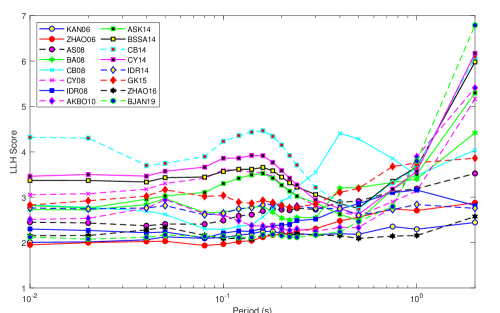
Figure 4: Plot of LLH score at 19 periods for the all the GMPEs considered in western and central Himalayas.

For clarity and easy visualization, the bar diagrams of LLH scores at three periods of importance for PSHA for all the GMPEs considered are presented in Fig. 5.

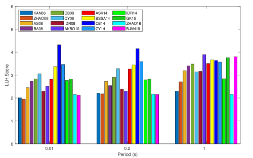
Figure 5: Bar diagram of LLH score at $0.01$s, $0.2$s and $1.0$s for the all the GMPEs considered in western and central Himalaya.

The distribution of normalized residuals, the best fit normal distribution (continuous curve) with the standard normal distribution (dashed curve) and the corresponding histograms of the LH values are presented in Fig. 6 for the suitable GMPEs at periods $0.01$ s, $0.2$ s and $1.0$ s respectively. It may be noted that the median $LH$ values and the $LLH$ scores are consistent for all the suitable set of GMPEs.

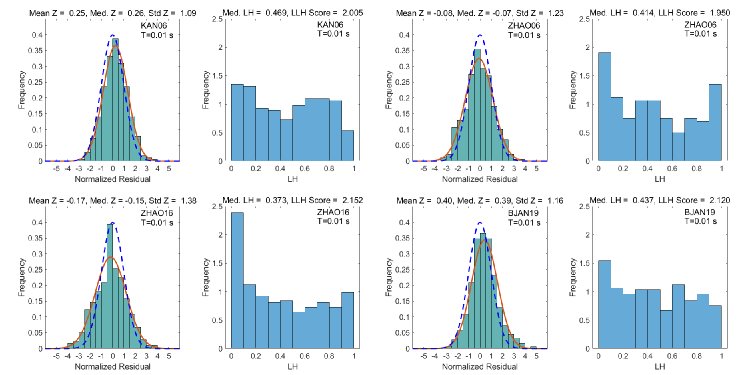
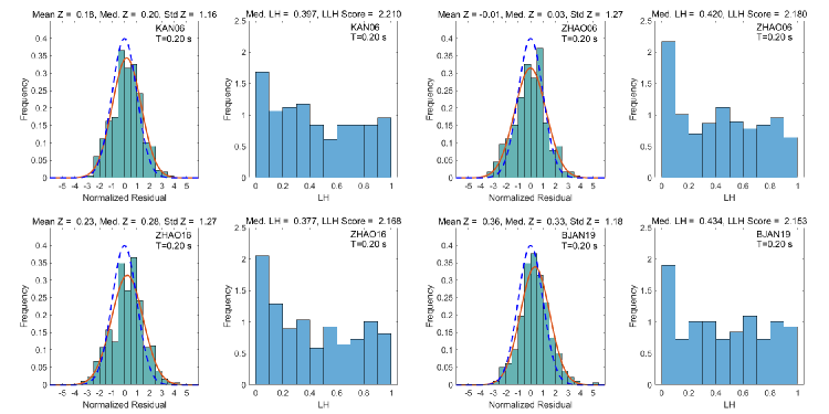
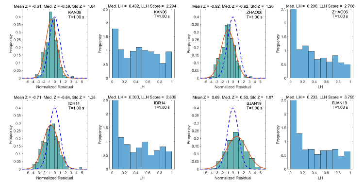
Figure 6: Left panel of each subfigure: Graph showing the distribution of normalized residual and the best fit normal distribution (continuous curve) with the standard normal distribution (dashed curve) at three periods of interest for four best suitable GMPEs in western and central Himalayas. Right side of each subfigure: Corresponding histograms of the LH values with the median LH and LLH score.

6.2 Results for Indo-Gangetic Plains

Table LABEL:reIG presents the overall summary of the goodness-of-fit parameters at $9$ different periods for all the GMPEs considered.

Table 5: Various goodness-of-fit measures for all the GMPEs considered in Indo-Gangetic Plains

GMPEs	Goodness-of-fit					Periods (s)
Considered	measures	0.01	0.02	0.05	0.10	0.20	0.30	0.50	1.00	2.00
KAN06	Mean $Z$	0.51	0.62	1.02	0.33	-0.15	-0.58	-0.88	-1.15	-1.10
	Median $Z$	0.55	0.69	1.05	0.32	-0.09	-0.74	-0.90	-1.27	-1.22
	Std $Z$	0.89	0.91	1.04	0.86	1.14	1.25	1.21	1.06	0.84
	Med. $LH$	0.47	0.43	0.29	0.54	0.40	0.33	0.22	0.20	0.22
	Rank	C	C	D	B	B	C	D	D	D
	$LLH$ Score	1.85	1.96	2.63	1.82	2.16	2.53	2.84	3.00	2.55
ZHAO06	Mean $Z$	0.15	0.13	0.73	0.18	-0.45	-1.19	-1.85	-1.85	-1.83
	Median $Z$	0.20	0.15	0.75	0.22	-0.45	-1.45	-1.93	-2.13	-2.04
	Std $Z$	1.04	1.03	1.12	0.94	1.29	1.47	1.54	1.41	1.10
	Med. $LH$	0.46	0.51	0.34	0.55	0.31	0.13	0.05	0.03	0.04
	Rank	A	A	D	A	C	D	D	D	D
	$LLH$ Score	1.65	1.67	2.25	1.75	2.37	3.51	5.09	4.86	4.25
AS08	Mean $Z$	-0.65	-0.54	-0.01	-0.60	-1.20	-1.63	-1.89	-2.08	-1.61
	Median $Z$	-0.65	-0.52	-0.01	-0.55	-1.23	-1.84	-1.91	-1.96	-1.43
	Std $Z$	1.18	1.17	1.10	1.29	1.59	1.57	1.44	1.30	1.17
	Med. $LH$	0.32	0.39	0.45	0.33	0.16	0.06	0.06	0.05	0.15
	Rank	C	C	A	C	D	D	D	D	D
	$LLH$ Score	2.11	1.99	1.82	2.45	3.81	4.62	4.96	5.17	3.65
BA08	Mean $Z$	0.01	0.16	0.97	0.06	-0.71	-1.34	-2.19	-2.20	-1.34
	Median $Z$	0.05	0.16	0.87	-0.06	-0.70	-1.24	-2.21	-2.18	-1.37
	Std $Z$	1.47	1.49	1.67	1.36	1.55	1.50	1.66	1.30	1.20
	Med. $LH$	0.29	0.32	0.18	0.37	0.28	0.15	0.03	0.03	0.16
	Rank	C	C	D	C	D	D	D	D	D
	$LLH$ Score	2.04	2.10	3.24	1.94	2.66	3.50	6.04	5.41	3.15
CB08	Mean $Z$	-0.73	-0.57	0.18	-0.54	-1.50	-2.25	-2.78	-2.45	-1.60
	Median $Z$	-0.65	-0.50	0.07	-0.51	-1.34	-2.38	-2.67	-2.53	-1.60
	Std $Z$	1.36	1.37	1.51	1.21	1.73	1.92	1.97	1.49	1.13
	Med. $LH$	0.33	0.36	0.33	0.36	0.14	0.02	0.01	0.01	0.11
	Rank	C	C	D	C	D	D	D	D	D
	$LLH$ Score	2.08	1.98	2.16	1.83	4.31	6.83	8.89	6.55	3.44
CY08	Mean $Z$	0.59	0.69	1.15	0.61	0.06	-0.38	-0.80	-1.30	-1.12
	Median $Z$	0.59	0.67	1.14	0.47	0.14	-0.39	-0.74	-1.17	-1.19
	Std $Z$	1.60	1.66	1.71	1.40	1.36	1.39	1.33	1.24	1.30
	Med. $LH$	0.23	0.20	0.15	0.31	0.38	0.37	0.29	0.23	0.20
	Rank	D	D	D	C	C	C	D	D	D
	$LLH$ Score	2.84	3.07	3.88	2.52	2.18	2.33	2.54	3.13	2.94
IDR08	Mean $Z$	-0.02	0.10	0.63	0.30	-0.31	-0.86	-1.29	-1.61	-1.32
	Median $Z$	0.12	0.18	0.64	0.51	-0.21	-0.89	-1.18	-1.62	-1.31
	Std $Z$	1.16	1.13	1.11	1.14	1.52	1.57	1.56	1.36	0.89
	Med. $LH$	0.46	0.49	0.38	0.40	0.26	0.23	0.14	0.11	0.19
	Rank	B	B	C	C	D	D	D	D	D
	$LLH$ Score	1.81	1.76	2.02	1.90	2.70	3.31	3.98	4.32	3.00
AKBO10	Mean $Z$	0.60	0.52	1.21	0.47	-0.32	-0.62	-0.63	-0.30	-0.01
	Median $Z$	0.75	0.67	1.10	0.62	-0.14	-0.42	-0.52	-0.29	-0.41
	Std $Z$	1.29	1.29	1.45	1.21	1.34	1.30	1.14	1.25	1.91
	Med. $LH$	0.34	0.34	0.19	0.36	0.38	0.30	0.45	0.42	0.26
	Rank	C	C	D	C	C	C	C	C	D
	$LLH$ Score	2.15	2.10	3.33	1.98	2.15	2.31	2.14	2.09	3.54
ASK14	Mean $Z$	1.08	1.08	1.54	1.01	0.43	0.05	-0.14	-0.03	0.14
	Median $Z$	1.16	1.20	1.42	1.00	0.43	0.04	-0.04	0.05	0.05
	Std $Z$	1.21	1.23	1.31	1.07	1.16	1.16	1.08	1.12	1.37
	Med. $LH$	0.18	0.17	0.12	0.27	0.38	0.44	0.48	0.47	0.42
	Rank	D	D	D	D	B	B	A	A	C
	$LLH$ Score	2.92	2.96	4.02	2.65	2.19	2.02	1.84	1.84	2.25
BSSA14	Mean $Z$	1.05	1.14	1.52	0.96	0.51	0.06	-0.36	-0.58	-0.40
	Median $Z$	1.07	1.21	1.53	0.92	0.66	0.14	-0.29	-0.60	-0.51
	Std $Z$	1.32	1.32	1.32	1.11	1.18	1.22	1.20	1.11	1.10
	Med. $LH$	0.18	0.18	0.12	0.27	0.34	0.36	0.45	0.43	0.37
	Rank	D	D	D	D	C	B	B	C	C
	$LLH$ Score	2.92	3.11	4.00	2.58	2.08	1.92	1.94	2.00	1.87
CB14	Mean $Z$	1.61	1.69	1.97	1.46	0.91	0.21	-0.30	-0.73	-0.57
	Median $Z$	1.83	1.89	2.04	1.52	0.97	0.26	-0.18	-0.65	-0.69
	Std $Z$	1.22	1.24	1.25	1.06	1.21	1.23	1.18	1.12	1.18
	Med. $LH$	0.07	0.06	0.04	0.12	0.25	0.35	0.45	0.39	0.34
	Rank	D	D	D	D	D	B	B	C	C
	$LLH$ Score	3.87	4.10	5.00	3.39	2.61	2.03	1.95	2.17	2.08
CY14	Mean $Z$	1.13	1.24	1.63	1.07	0.59	0.08	-0.25	-0.53	-0.53
	Median $Z$	1.06	1.24	1.61	0.94	0.64	0.14	-0.24	-0.50	-0.67
	Std $Z$	1.21	1.25	1.39	1.09	1.14	1.13	1.04	1.02	1.16
	Med. $LH$	0.19	0.14	0.10	0.23	0.38	0.39	0.48	0.44	0.34
	Rank	D	D	D	D	C	B	B	C	C
	$LLH$ Score	2.88	3.13	4.25	2.67	2.20	1.97	1.88	1.95	2.08
IDR14	Mean $Z$	-0.88	-0.80	-0.04	-0.61	-1.20	-1.61	-1.82	-2.23	-1.82
	Median $Z$	-0.86	-0.74	-0.23	-0.62	-1.18	-1.69	-1.87	-2.38	-2.09
	Std $Z$	1.37	1.32	1.22	1.31	1.67	1.78	1.75	1.73	1.25
	Med. $LH$	0.21	0.24	0.43	0.36	0.13	0.07	0.06	0.02	0.04
	Rank	D	D	B	C	D	D	D	D	D
	$LLH$ Score	2.83	2.65	2.00	2.49	4.06	5.19	5.67	6.85	4.69
GK15	Mean $Z$	0.52	0.66	1.10	0.43	-0.24	-0.86	-1.55	-2.27	-2.25
	Median $Z$	0.24	0.36	0.61	0.14	-0.13	-0.74	-1.36	-2.13	-2.40
	Std $Z$	1.60	1.68	1.93	1.53	1.53	1.66	1.74	1.64	1.31
	Med. $LH$	0.36	0.34	0.25	0.34	0.30	0.18	0.10	0.03	0.02
	Rank	D	D	D	D	D	D	D	D	D
	$LLH$ Score	2.74	3.02	4.25	2.52	2.44	3.24	4.70	6.63	6.05
ZHAO16	Mean $Z$	0.00	0.07	0.35	-0.23	-0.37	-0.68	-0.94	-1.09	-1.02
	Median $Z$	0.02	0.09	0.42	-0.18	-0.20	-0.77	-0.94	-1.13	-1.12
	Std $Z$	1.17	1.16	1.19	1.09	1.32	1.39	1.46	1.36	1.10
	Med. $LH$	0.46	0.46	0.43	0.46	0.32	0.28	0.22	0.20	0.23
	Rank	B	B	B	A	C	D	D	D	D
	$LLH$ Score	1.75	1.74	1.98	1.87	2.32	2.66	3.08	3.14	2.50
BJAN19	Mean $Z$	1.08	0.99	0.99	0.64	0.57	0.38	0.55	0.68	1.55
	Median $Z$	1.06	0.84	0.58	0.57	0.57	0.37	0.63	0.76	0.95
	Std $Z$	1.25	1.28	1.41	1.04	1.06	1.10	1.11	1.18	2.31
	Med. $LH$	0.20	0.29	0.31	0.42	0.38	0.34	0.34	0.32	0.21
	Rank	D	D	D	C	C	B	C	D	D
	$LLH$ Score	3.00	3.00	3.37	2.29	2.10	1.98	2.05	2.25	6.46

It is apparent from Table LABEL:reIG that each goodness-of-fit parameters show appreciable variation over periods for all the GMPEs. Moreover, no single GMPE can be considered suitable for the entire range of spectral periods in this target region. For different periods of interest, different set of GMPEs are suitable to construct the logic trees in PSHA. For PGA ($0.01$ s), it is suggested to use ZHAO06, IDR08, ZHAO16 and KAN06. For $0.2$ s, our analysis shows that a combination of BSSA14, BJAN19, AKBO10 and KAN06 may be considered suitable for constructing the logic tree. LLH score is given more importance in selecting these set of GMPEs as LLH score is sample size independent. For $1.0$ s, the combination of ASK14, BSSA14, CY14 and AKBO10 may be considered appropriate for designing of logic tree. The variation of LLH score at $20$ periods is plotted in Fig. 7 and the bar diagrams of LLH scores at the three periods of importance for all the GMPEs are shown in Fig. 8 for easy understanding.

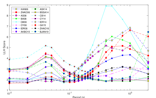
Figure 7: Plot of LLH score at 19 periods for the all the GMPEs considered in Indo-Gangetic Plains.

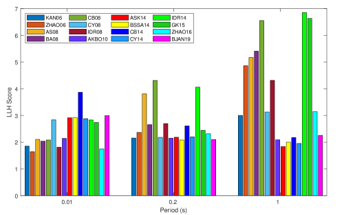
Figure 8: Bar diagram of LLH score at $0.01$s, $0.2$s and $1.0$s for the all the GMPEs considered in Indo-Gangetic Plains.

In general, it is observed that for this region NGA-West2 GMPEs perform better than the NGA-West1 GMPEs for periods $\geq$ $0.2$ s except for IDR14. The distribution of normalized residuals, the best fit normal distribution (continuous curve) with the standard normal distribution (dashed curve) and the corresponding histograms of the LH values are presented in Fig. 9 for the suitable GMPEs at periods $0.01$ s, $0.2$ s and $1.0$ s respectively. It may be noted that the median $LH$ values and the $LLH$ scores behave consistently for all the suitable set of GMPEs in this target region, too.

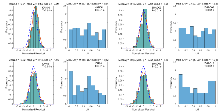
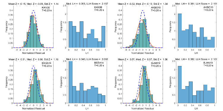
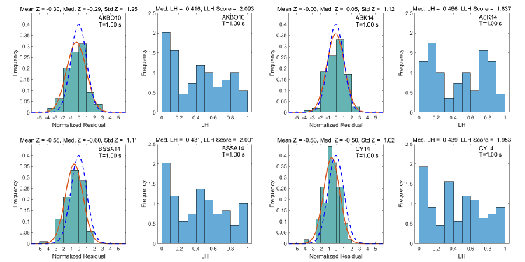
Figure 9: Left panel of each subfigure: Graph showing the distribution of normalized residual and the best fit normal distribution (continuous curve) with the standard normal distribution (dashed curve) at three periods of interest for four best suitable GMPEs in Indo-Gangetic Plains. Right side of each subfigure: Corresponding histograms of the LH values with the median LH and LLH score.

7 Conclusion

With the ever-increasing number of GMPEs with time, the selection of suitable GMPEs for the construction of logic trees in SHA for a target region has become a necessity. The construction of logic trees is a standard practice to address the epistemic uncertainties associated with various input parameters. These uncertainties are relatively larger in regions where limited number of recorded ground motion are available. However, this data limitation should not be used as a basis by the hazard analysts to indulge in subjectivities while selecting suitable set of GMPEs for carrying out hazard calculations. Bommer et al. (2010) pointed out that the selection process “should neither be guided by familiarity with certain GMPEs nor by any particular preference that the analyst may have for a given model”. Rather, the appropriateness of GMPEs should be judged by data-driven methods which are based on sound mathematical background.

To this end, this paper has focused on the selection of the best possible GMPEs by carrying out a thorough analysis in two geo-tectonic units which are characterized by distinct geophysical and geo-technical properties. For the analysis of suitability of GMPEs, two widely used data-driven methods proposed by Scherbaum et al. (2004) and Scherbaum et al. (2009) are considered. Given the amount of available data, different suites of suitable GMPEs are suggested to be used for different periods of interest in these two target regions. The results of the ranking of the GMPEs from both the methods are very consistent. The weight factor to be assigned to each selected GMPE for construction of logic tree is a separate topic, which is left for future research. However, in the present case, the weight factor to each suitable GMPE for a particular target region may be decided from the LLH score following the prescription given in Scherbaum et al. (2009), if the readers wish. The regions under study have witnessed a number of significant earthquakes in the recent past and therefore data-driven selection and ranking of appropriate GMPEs for SHA in these regions is a necessity. We believe that the results obtained from this research will help the scientists and engineers entrusted with the task of microzonation and earthquake-resistant design of structures in these regions. The paper is not intended to make any judgement about any particular GMPE being superior or inferior to any other. Our aim is to provide a data-driven selection and ranking of GMPEs that predict the observed ground-motion best in these target regions, given the available data at our disposal.

Disclosure statement

The authors have no conflicts of interest to declare that are relevant to the content of this article.

Data availability statement

All the data used in this research are available in public domain and the links for accessing the data are given inside the text.

Funding details

No funding was received for conducting this study.

References

- Abrahamson and Silva (2008) Abrahamson NA, Silva WJ (2008) Summary of the Abrahamson and Silva NGA GRound Motion Relations. Earthquake Spectra 24:67–197
- Abrahamson et al. (2014) Abrahamson NA, Silva WJ, Kamai R (2014) Summary of the ASK14 ground motion relation for active crustal regions. Earthquake Spectra 30(3):1025–1055
- Akkar and Bommer (2010) Akkar S, Bommer J (2010) Empirical equations for the prediction of pga, pgv, and spectral accelerations in Europe, the Mediterranean region, and the Middle East. Seismological Research Letters 81(2):195–206
- Anbazhagan et al. (2015) Anbazhagan P, Bajaj K, Moustafa SSR, Al-Arifi NSN (2015) Maximum magnitude estimation considering the regional rupture character. Journal of Seismology 19:695–719
- Arango et al. (2012) Arango MC, Free MW, Lubkowski ZA, Pappin JW, Musson RMW, Jones G, Hodge E (2012) Comparing predicted and observed ground motions from UK earthquakes. In: 15th World Conf. on Earthquake Engineering
- B. Naresh and Mishra (2021) B Naresh KV, Mishra LK (2021) The seismotectonic setting of indo-gangetic plain and its importance. In: Seismic Hazards and Risk: Select Proceedings of 7th ICRAGEE 2020 (Lecture Notes in Civil Engineering), vol 116, pp 187–196
- Bajaj and Anbazhagan (2019) Bajaj K, Anbazhagan P (2019) Regional stochastic GMPE with available recorded data for active region – application to the Himalayan region. Soil Dynamics and Earthquake Engineering 126:105825
- Beauval et al. (2012) Beauval C, Tasan H, Laurendeau A, Delavaud E, Cotton F, Gueguen P, Kuehn N (2012) On the testing of ground-motion prediction equations against small magnitude data. Bull Seism Soc Am 102:1994–2007
- Bommer and Scherbaum (2008) Bommer JJ, Scherbaum F (2008) The use and misuse of logic-trees in PSHA. Earthquake Spectra 24:997–1009
- Bommer et al. (2010) Bommer JJ, Douglas J, Scherbaum F, Cotton F, Bungum H, Fah D (2010) On the selection of ground-motion prediction equations for seismic hazard analysis. Seismological Research Letters 81:783–793
- Boore et al. (2014) Boore DM, Stewart JP, Seyhan E, Atkinson GM (2014) NGA-West2 equations for predicting pga, pgv, and 5 damped psa for shallow crustal earthquakes. Earthquake Spectra 30(3):1057 – 1085
- Boore and Atkinson (2008) Boore MD, Atkinson GM (2008) Ground-motion prediction equations for the average horizontal component of PGA, PGV, and 5-damped PSA at spectral periods between 0.01 s and 10.0s. Earthquake Spectra 24:99–138
- Bykova (2016) Bykova VV (2016) On the selection of ground-motion prediction equations during the assessment of seismic hazard in stable continental regions. Seismic Instruments 52:135–143
- Campbell and Bozorgnia (2008) Campbell KW, Bozorgnia Y (2008) NGA ground motion model for the geometric mean horizontal component of PGA, PGV, PGD and 5 damped linear elastic response spectra for periods ranging from 0.01 to 10s. Earthquake Spectra 24:139–171
- Campbell and Bozorgnia (2014) Campbell KW, Bozorgnia Y (2014) NGA-West2 ground motion model for the average horizontal components of pga, pgv, and 5 damped linear acceleration response spectra. Earthquake Spectra 30(3):1087 – 1115
- Chiou and Youngs (2008) Chiou B, Youngs RR (2008) An NGA model for the average horizontal component of peak ground motion and response spectra. Earthquake spectra 24:173–215
- Chiou and Youngs (2014) Chiou BSJ, Youngs RR (2014) Update of the chiou and youngs nga model for the average horizontal component of peak ground motion and response spectra. Earthquake Spectra 30(3):1117 – 1153
- Cotton et al. (2006) Cotton F, Scherbaum F, Bommer JJ, Bungum H (2006) Criteria for selecting and adjusting ground-motion models for specific target applications: Applications to central europe and rock sites. Journal of Seismology 10:137–156
- Cover and Thomas (2006) Cover TM, Thomas JA (2006) Elements of Information Theory, Second ed., Wiley, Hoboken, New Jersey
- Dasgupta et al. (2000) Dasgupta S, Pande P, Ganguly D, Iqbal Z, Sanyal K, Venaktraman NV, Dasgupta S, Sural B, Harendranath L, Mazumdar K, Sanyal S, Roy A, Das LK, Misra PS, Gupta H (2000) Seismotectonic Atlas of India and Its Environs. Geological Survey of India:Calcutta
- Delavaud et al. (2009) Delavaud E, Scherbaum F, Kuehn N, Riggelsen C (2009) Information- theoretic selection of ground-motion prediction equations for seismic hazard analysis: An applicability study using California data. Bull Seism Soc Am 99:3248–3263
- Douglas (2007) Douglas J (2007) On the regional dependence of earthquake response spectra. ISET Journal of Earthquake Technology 44:71–99
- Douglas (2022) Douglas J (2022) Ground motion prediction equations 1964-2021. http://www.gmpe.org.uk
- Edwards (1992) Edwards AWF (1992) Likelihood, Expanded ed., Johns Hopkins Univ. Press
- Graizer and Kalkan (2016) Graizer V, Kalkan E (2016) Summary of GK15 ground-motion prediction equation for predicting PGA and 5 damped SA from shallow crustal continental earthquakes. Bulletin of Seismological Society of America 106(2):687–707
- Gupta (2006) Gupta ID (2006) Delineation of probable seismic sources in india and neighbourhood. Soil Dynamics and Earthquake Engineering 26:766–790
- Gupta and Trifunac (2018) Gupta ID, Trifunac MD (2018) Empirical scaling relations for pseudo relative veocity spectra in western Himalaya and northeastern India. Soil Dynamics and Earhquake engineering 106:70–89
- Hintersberger et al. (2007) Hintersberger E, Scherbaum F, Hainzl S (2007) Update of likelihood-based ground-motion model selection for seismic hazard analysis in western central Europe. Bull Earth Engg 5:1–16
- Idriss (2008) Idriss IM (2008) An NGA empirical model for estimating the horizontal spectral values generated by shallow crustal earthquakes. Earthquake Spectra 24(1):217–242
- Idriss (2014) Idriss IM (2014) An NGA-West2 empirical model for estimating the horizontal spectral values generated by shallow crustal earthquakes. Earthquake Spectra 30(3):1155 – 1177
- Kale and Akkar (2013) Kale O, Akkar S (2013) A new procedure for selecting and ranking ground-motion prediction equations (gmpes): The Euclidean distance-based ranking (EDR) method. Bull Seism Soc Am 103:1069–1084
- Kanno et al. (2006) Kanno T, Narita A, Morikawa N, Fujiwara H, Fukushima Y (2006) A new attenuation releation for strong ground motion in Japan based on recorded data. Bulletin of the seismological Society of America 96:879–897
- Kayal (2010) Kayal JR (2010) Himalayan tectonic model and the great earthquakes: an appraisal. Geomatics, Natural Hazards and Risk 1(1):51–67
- Kayal (2014) Kayal JR (2014) Seismotectonics of the great and large earthquakes in himalaya. Current Science 106(2):188–197
- Kayal et al. (2022) Kayal JR, Baruah S, Hazarika D, Das A (2022) Recent large and strong earthquakes in the eastern himalayas: An appraisal on seismotectonic model. Geological Journal 57(12):4929–4938
- Kowsari et al. (2019) Kowsari M, Halldorsson B, Hrafnkelsson B, Jonsson S (2019) Selection of earthquake ground motion models using the deviance information criterion. Soil Dynam Earthq Engg 117:288–299
- Kulkarni et al. (1984) Kulkarni RB, Youngs RR, Coppersmith KJ (1984) Assessment of confidence intervals for results of seismic hazard analysis. In: 8th World Conf. on Earthquake Engineering, pp 263–270
- Kumar et al. (2016) Kumar A, Singh S, Mitra S, Priestly KF, Dayal S (2016) The 2015 April 25 Gorkha (Nepal) earthquake and its aftershocks: implications for lateral heterogeneity of the Main Himalayan Thrust. Geophysical Journal International 208(2):992–1008
- Nath et al. (2012) Nath SK, Thingbaijam K, Maity S, Nayak A (2012) Ground-motion predictions in Shilong region, North-East India. Journal of Seismology 16:475–488
- Nayak and Sitharam (2019) Nayak M, Sitharam TG (2019) Estimation and spatial mapping of seismicity parameters in western Himalaya, central Himalaya and Indo-Gangetic plain. J Earth Syst Sci 128:45
- Nh and Kumar (2020) Nh H, Kumar A (2020) Ground motion prediction equation for north India, applicabale for different site classes. Soil Dynamics and Earhquake engineering 139:106425
- Scherbaum et al. (2004) Scherbaum F, Cotton F, Smit P (2004) On the use of response spectral-reference data for the selection and ranking of ground-motion models for seismic-hazard analysis in regions of moderate seismicity: The case of rock motion. Bull Seism Soc Am 94:2164–2185
- Scherbaum et al. (2009) Scherbaum F, Delavaud E, Riggelsen C (2009) Model selection in seismic hazard analysis: an information- theoretic perspective. Bull Seism Soc Am 99:3234–3247
- Sharma et al. (2009) Sharma ML, Douglas J, Bungum H, Kotadia J (2009) Groung motion prediction equations based on data from the Himalayan and Zagros region. Journal of Earthquaje Engineering 13:1191–1210
- Singh et al. (2017) Singh SK, Srinagesh D, Srinivas D, Arroyo D, amd R K Chadha XPC, Suresh G, Suresh G (2017) Strong Ground Motion in the Indo-Gangetic Plains during the 2015 Gorkha, Nepal, Earthquake Sequence and Its Prediction during Future Earthquakes. Bulletin of the Seismological Society of America 107(3):1293–1306
- Sinha and Selvan (2022) Sinha S, Selvan S (2022) An improved probabilistic seismic hazard assessment of Tripura, India. Pure and Applied Geophysics 179:4371–4393
- Slejko and Rebez (2002) Slejko D, Rebez A (2002) Probabilistic seismic hazard assessment and deterministic ground shaking scenarios for Vittorio Veneto (N.E.Italy) volume = 43, journal = Boll. Geof. Teor. Appl., pp 263–280
- Stafford et al. (2008) Stafford PJ, Strasser FO, Bommer JJ (2008) An evaluation of the applicability of the nga models to ground-motion prediction in the euro-mediterranean region. Bulletin of Earthquake Engineering 6:149–177
- Strasser et al. (2009) Strasser FO, Abrahamson NA, Bommer JJ (2009) Sigma: Issues, insights and challenges. Seismological Research Letters 80:40–56
- Wessel et al. (2019) Wessel P, Luis FJ, Uieda L, Scharroo R, Wobbe F, Smith WHF, Tian D (2019) The Generic Mapping Tools version 6 pp 5556–5564
- Zhao et al. (2006) Zhao JX, Zhang J, Asano A, Ohno Y, Oouchi T, Takahashi T, Ogawa H, Irikura K, Thio HK, Somerville PG, Fukushima Y, Fukushima Y (2006) Attentuation relations of strong ground motion in Japan using site classification based on predominant period. Bulletin of the Seismological Society of America 96(3):898 – 913
- Zhao et al. (2016) Zhao JX, Zhou SL, Gao PJ, Zhang YB, Zhou J, Lu M, Rhoades DA (2016) Ground-motion prediction equations for shallow crustal and upper mantle earthquakes in Japan using site class and simple geometric attenuation functions. Bulletin of the Seismological Society of America 106:1552 – 1569