HaTT: Hadamard avoiding TT recompression

Abstract

The Hadamard product of tensor train (TT) tensors is one of the most fundamental nonlinear operations in scientific computing and data analysis. Due to its tendency to significantly increase TT ranks, the Hadamard product presents a major computational challenge in TT tensor-based algorithms. Therefore, it is essential to develop recompression algorithms that mitigate the effects of this rank increase. Existing recompression algorithms require an explicit representation of the Hadamard product, resulting in high computational and storage complexity. In this work, we propose the Hadamard avoiding TT recompression (HaTT) algorithm. Leveraging the structure of the Hadamard product in TT tensors and its Hadamard product-free property, the overall complexity of the HaTT algorithm is significantly lower than that of existing TT recompression algorithms. This is validated through complexity analysis and several numerical experiments.

1 Introduction

Tensor train (TT) decomposition, also known as matrix product states (MPS), is a powerful tool for dimension reduction in various applications such as scientific computing [14, 7, 4, 17, 23], machine learning [31, 26, 13, 28, 27], and quantum computing [29, 10, 32, 15]. With TT decomposition, a tensor of order $d$ can be represented as the product of $d$ core tensors of order no more than three, and its memory cost only grows linearly with $d$. More importantly, most algebraic operations in TT tensors can be converted into the corresponding operations on TT cores, significantly reducing computational complexity and overcoming the curse of dimensionality. Consequently, TT representation is one of the most efficient tensor networks for solving large-scale and high-dimensional problems [22, 4, 5, 20].

The Hadamard product is a fundamental operation in tensor-based algorithms for scientific computing and data analysis [18, 24, 8, 3, 9]. Implementing the Hadamard product for TT tensors can be converted into the partial Kronecker product (PKP) of TT cores, resulting in a quadratic increase in TT ranks. This rank growth leads to a significant increase in the complexity of the recompression algorithm. For sufficiently large TT tensors, this operation and the subsequent recompression can dominate computational time. Therefore, developing efficient recompression techniques for Hadamard product that mitigate the effects of rank increase is of significant interest.

Related work. The widely used recompression algorithm for TT tensors is the TT-Rounding algorithm [22], which consists of two parts: orthogonalization and compression (typically using the SVD). For a given TT tensor with maximal rank $r$, the computational cost of the TT-Rounding algorithm is on the order of $r^{3}$, making it inefficient for TT tensors with large $r$, such as the Hadamard product of TT tensors. To enhance the performance of TT-Rounding algorithm, several parallel approaches based on randomized sketching have been proposed [6, 1, 30, 25]. To avoid the expensive orthogonalization step in TT-Rounding, three randomized algorithms were introduced by generalizing randomized low-rank matrix approximation [2]. One of these algorithms, named Randomize-then-Orthogonalize (RandOrth), offers the best speedup compared to the deterministic TT-Rounding algorithm and is probably the state-of-the-art method for TT recompression.

Our contributions. In this work, we design a Hadamard avoiding TT recompression (HaTT) algorithm to recompress the Hadamard product $\bm{\mathcal{A}}:=\bm{\mathcal{Y}}\odot\bm{\mathcal{Z}}$ of two TT tensors. This method avoids the explicit calculation of the Hadamard product $\bm{\mathcal{A}}$, significantly reducing the overall computation cost of the rounding procedure compared to all existing TT recompression algorithms. In the HaTT algorithm, we first obtain the sketching matrices by partially contracting $\bm{\mathcal{A}}$ and a random tensor $\bm{\mathcal{R}}$. By utilizing the PKP structure in TT cores of $\bm{\mathcal{A}}$, these sketching matrices can be computed from TT cores of $\bm{\mathcal{Y}}$ and $\bm{\mathcal{Z}}$, thus avoiding the explicit computation of the TT cores of $\bm{\mathcal{A}}$. We then perform the orthogonalization sweep to construct a low rank TT tensor approximation for $\bm{\mathcal{A}}$. During this process, the PKP structure is also applied, allowing the orthogonalization sweep to be directly implemented from the TT cores of $\bm{\mathcal{Y}}$ and $\bm{\mathcal{Z}}$. In summary, the HaTT algorithm recompresses the Hadamard product $\bm{\mathcal{A}}$ by avoiding explicit calculation and storage of $\bm{\mathcal{A}}$. Based on the complexity analysis, the computational cost of the HaTT algorithm is almost $r$ times less than that of the RandOrth algorithm (see Section 3.3), where $r$ is the maximal rank of $\bm{\mathcal{Y}}$ or $\bm{\mathcal{Z}}$. Numerical experiments (see Section 4) exhibit a significant speedup for the HaTT algorithm compared to all widely used TT recompression algorithms.

2 Background

2.1 Tensor notations and operations

In this paper, we use the bold lowercase letter to represent a vector (e.g., $\bm{x}$), the bold uppercase letter to represent a matrix (e.g., $\bm{X}$), and the bold script letter to represent a tensor (e.g., $\bm{\mathcal{X}}$), respectively. For a $d$th-order tensor $\bm{\mathcal{X}}\in\mathbb{R}^{n_{1}\times n_{2}\times\dots\times n_{d}}$, its $(i_{1},i_{2},\dots,i_{d})$th element is denoted as $\bm{\mathcal{X}}(i_{1},i_{2},\dots,i_{d})$ or $x_{i_{1},i_{2},\dots,i_{d}}$, and the Frobenius norm of $\bm{\mathcal{X}}$ is defined as $\left\|\bm{\mathcal{X}}\right\|_{\mathrm{F}}=\sqrt{\sum_{i_{1},i_{2},\ldots,i_{d}=1}^{n_{1},n_{2},\ldots,n_{d}}\left|\bm{\mathcal{X}}(i_{1},i_{2},\dots,i_{d})\right|^{2}}$.

We then introduce several folding and unfolding operators for vector, matrix, and tensor. For the sake of convenience, we define the multi-index as $\overline{i_{1}i_{2}\cdots i_{d}}=i_{d}+(i_{d-1}-1)n_{d}+\cdots+(i_{1}-1)n_{2}\cdots n_{d}$. The vectorization operator vectorizes a matrix $\bm{X}\in\mathbb{R}^{m\times n}$ into a column vector $\text{vec}(\bm{X})\in\mathbb{R}^{mn}$ with $\text{vec}(\bm{X})=(x_{1,1},x_{2,1},\dots,x_{m,1},x_{1,2},\dots,x_{m,2},x_{1,3},\dots,x_{m,n})^{\mathsf{T}}.$ Correspondingly, the matricization operator folds a vector $\bm{x}\in\mathbb{R}^{mn}$ into a matrix $\bm{X}=\bm{x}|_{n}^{m}\in\mathbb{R}^{m\times n}$ with $\bm{X}(:,1)=(x_{1},x_{2},\dots,x_{m})^{\mathsf{T}}$, $\bm{X}(:,2)=(x_{m+1},x_{m+2},\dots,x_{2m})^{\mathsf{T}}$, and so on. Vectorization and matricization can be generalized to tensors. For example, the mode-$(1,2,\dots,k)$ matricization of $\bm{\mathcal{X}}$ reshapes it to a matrix $\unfold{X}{k}\in\mathbb{R}^{(n_{1}\cdots n_{k})\times(n_{k+1}\cdots n_{d})}$ that satisfies $\unfold{X}{k}(\overline{i_{1}i_{2}\ldots i_{k}},\overline{i_{k+1}i_{k+2}\ldots i_{d}})=\bm{\mathcal{X}}(i_{1},i_{2},\dots,i_{d}).$ In particular, we denote $\unfold{X}{1}$ and $\unfold{X}{d-1}$ as $\HT{\bm{\mathcal{X}}}$ and $\VT{\bm{\mathcal{X}}}$, which are called horizontal and vertical matricization.

The Kronecker and Hadamard products of tensors are denoted as $\otimes$ and $\odot$, respectively. Let $\bm{\mathcal{Y}},\bm{\mathcal{Z}}\in\mathbb{R}^{n_{1}\times n_{2}\times\dots\times n_{d}}$ and $\bm{\mathcal{Q}}\in\mathbb{R}^{m_{1}\times m_{2}\times\dots\times m_{d}}$ be $d$th-order tensors, $\bm{\mathcal{X}}\otimes\bm{\mathcal{Q}}$ and $\bm{\mathcal{X}}\odot\bm{\mathcal{Y}}$ are specifically defined as

$$\bm{\mathcal{A}} =\bm{\mathcal{Y}}\otimes\bm{\mathcal{Q}}, \bm{\mathcal{A}}(\overline{i_{1}j_{1}},\overline{i_{2}j_{2}},\dots ,\overline{i_{d}j_{d}})=\bm{\mathcal{Y}}(i_{1},i_{2},\dots,i_{d})\cdot\bm{\mathcal{Q}}(j_{1},j_{2},\dots,j_{d}),$$

$$\bm{\mathcal{A}} =\bm{\mathcal{Y}}\odot\bm{\mathcal{Z}}, \bm{\mathcal{A}}(i_{1},i_{2},\dots,i_{d}) =\bm{\mathcal{Y}}(i_{1},i_{2},\dots,i_{d})\cdot\bm{\mathcal{Z}}(i_{1},i_{2},\dots,i_{d}).$$

For the Kronecker product of matrices, the following important property will be used in this paper:

$$(\bm{A}\otimes\bm{B})\bm{v}=\text{vec}\left(\bm{B}\bm{V}\bm{A}^{\mathsf{T}}\right),$$ (1)

where $\bm{A}\in\mathbb{R}^{m\times n}$, $\bm{B}\in\mathbb{R}^{r\times s}$, $\bm{v}\in\mathbb{R}^{ns}$, and $\bm{V}=\bm{v}|_{n}^{s}$.

The PKP is the Kronecker product of tensors along specified modes [19]. For two third-order tensors $\bm{\mathcal{Y}}\in\mathbb{R}^{r_{1}\times n\times r_{2}}$ and $\bm{\mathcal{Z}}\in\mathbb{R}^{s_{1}\times n\times s_{2}}$, the PKP of them along mode-1 and -3 is denoted as $\bm{\mathcal{A}}=\left(\bm{\mathcal{Y}}\boxtimes^{1,3}\bm{\mathcal{Z}}\right)\in\mathbb{R}^{r_{1}s_{1}\times n\times r_{2}s_{2}}$, i.e., $\bm{\mathcal{A}}(\overline{\alpha_{1}\beta_{1}},i,\overline{\alpha_{2}\beta_{2}})=\bm{\mathcal{Y}}(\alpha_{1},i,\alpha_{2})\cdot\bm{\mathcal{Z}}(\beta_{1},i,\beta_{2})$.

Let $\bm{\mathcal{X}}\in\mathbb{R}^{n_{1}\times n_{2}\times\cdots\times n_{d}},\bm{\mathcal{Y}}\in\mathbb{R}^{m_{1}\times m_{2}\times\cdots\times m_{l}}$ be two tensors that satisfy $n_{d-k+s}=m_{s}$ for all $s=1,\cdots,k$, we denote the contraction of $\bm{\mathcal{X}}$ and $\bm{\mathcal{Y}}$ along indices $\{d-k+1,\ldots,d\}$ and $\{1,2,\cdots,k\}$ as $\bm{\mathcal{Z}}=\left(\bm{\mathcal{X}}\times^{1,\ldots,k}\bm{\mathcal{Y}}\right)\in\mathbb{R}^{n_{1}\times\cdots\times n_{d-k}\times m_{k+1}\times\cdots\times m_{l}}$, elementwisely,

$$\begin{split}\bm{\mathcal{Z}}(i_{1},\ldots,i_{d-k},j_{k+1},\ldots,j_{l})=\sum\limits_{\alpha_{1},\ldots,\alpha_{k}=1}^{m_{1},\ldots,m_{k}}\bm{\mathcal{X}}(i_{1},\ldots,i_{d-k},\alpha_{1},\ldots,\alpha_{k})\cdot\bm{\mathcal{Y}}(\alpha_{1},\ldots,\alpha_{k},j_{k+1},\ldots,j_{l}).\end{split}$$

2.2 TT tensor and the Hadamard product

The TT decomposition represents $\bm{\mathcal{X}}$ as the product of $d$ tensors of order at most three, i.e.,

$$\bm{\mathcal{X}}=\bm{\mathcal{T}}_{\bm{\mathcal{X}},1}\times^{1}\bm{\mathcal{T}}_{\bm{\mathcal{X}},2}\times^{1}\dots\times^{1}\bm{\mathcal{T}}_{\bm{\mathcal{X}},d},$$ (2)

where $\{\bm{\mathcal{T}}_{\bm{\mathcal{X}},k}\in\mathbb{R}^{r_{k-1}\times n_{k}\times r_{k}}:k=1,2,\dots,d\}$ are called TT cores, and $r_{0}=r_{d}=1,r_{1},\dots,r_{d-1}$ are the TT ranks of $\bm{\mathcal{X}}$. For convenience, we call a tensor represented by the TT decomposition (2) as a TT tensor, which can be represented by a tensor network diagram (see Fig. 1).

Figure 1: Tensor network diagram for a TT tensor $\bm{\mathcal{X}}$.

Particularly, if the mode-$1$ (-$3$) matricization of the $k$th TT core $\bm{\mathcal{T}}_{\bm{\mathcal{X}},k}$ satisfies row (column) orthogonality, we call $\bm{\mathcal{T}}_{\bm{\mathcal{X}},k}$ is left (right) orthogonal. In addition, we define the partial contracted product $\bm{\mathcal{T}}_{\bm{\mathcal{X}},k:l}$ for $1\leq k<l\leq d$ as

$$\bm{\mathcal{T}}_{\bm{\mathcal{X}},k:l} =\bm{\mathcal{T}}_{\bm{\mathcal{X}},k}\times^{1}\bm{\mathcal{T}}_{\bm{\mathcal{X}},2}\times^{1}\dots\times^{1}\bm{\mathcal{T}}_{\bm{\mathcal{X}},l}\in\mathbb{R}^{r_{k-1}\times n_{k}\times\dots\times n_{l}\times r_{l}}.$$

With TT representation, the memory cost of $\bm{\mathcal{X}}$ can be reduced from $\prod_{k=1}^{d}n_{k}$ to $\sum_{k=1}^{d}n_{k}r_{k-1}r_{k}$, which grows linearly with $d$. More importantly, the basic operations of TT tensors can be converted into the corresponding operations on TT cores.

Let us consider the Hadamard product of TT tensors $\bm{\mathcal{A}}:=\bm{\mathcal{Y}}\odot\bm{\mathcal{Z}}$, where TT tensors $\bm{\mathcal{Y}},\bm{\mathcal{Z}}\in\mathbb{R}^{n_{1}\times\cdots\times n_{d}}$ with TT ranks $\{r_{k}\}_{k=0}^{d}$ and $\{s_{k}\}_{k=0}^{d}$, respectively. Assume that we need to recompress $\bm{\mathcal{A}}$ to a TT tensor with ranks $\{\ell_{k}\}_{k=0}^{d}$. For the sake of convenience, we denote $n=\max_{1\leq k\leq d}n_{k}$, $r=\max_{1\leq k\leq d}r_{k},$ $s=\max_{1\leq k\leq d}s_{k},$ and $\ell=\max_{1\leq k\leq d}\ell_{k}$, respectively. We further assume that $\ell<rs$. The $k$th TT core of the Hadamard product $\bm{\mathcal{A}}=\bm{\mathcal{Y}}\odot\bm{\mathcal{Z}}$ can be obtained by $\bm{\mathcal{T}}_{\bm{\mathcal{A}},k}=\bm{\mathcal{T}}_{\bm{\mathcal{Y}},k}\boxtimes^{1,3}\bm{\mathcal{T}}_{\bm{\mathcal{Z}},k}$. It is worth noting that the TT ranks of $\bm{\mathcal{A}}$ will increase to $\{r_{k}s_{k}\}_{k=0}^{d}$, which leads to a significant increase in the complexity of the recompression algorithm. The most popular recompression algorithm is TT-Rounding proposed in [22], which consists of two steps: orthogonalization and recompression. The computational procedure of TT-Rounding algorithm is shown in Algorithm 3. To recompress the TT tensor $\bm{\mathcal{A}}$ using the TT-Rounding algorithm, the total computational cost is $(d-2)n(5r^{3}s^{3}+6r^{2}s^{2}\ell+2rs\ell^{2})$, which is quite expensive, especially for tensors $\bm{\mathcal{Y}}$ and $\bm{\mathcal{Z}}$ with relatively large ranks. Similar challenges exist for other recompression algorithms and the corresponding complexity is displayed in Table 1.

3 Hadamard avoiding TT recompression

In this section, we establish a HaTT algorithm to efficiently round the Hadamard product $\bm{\mathcal{A}}=\bm{\mathcal{Y}}\odot\bm{\mathcal{Z}}$ into a TT tensor with ranks $\{\ell_{k}\}_{k=0}^{d}$. Inspired by RandOrth [2] (see Appendix C), the HaTT algorithm recompresses $\bm{\mathcal{A}}$ using the partial contraction of $\bm{\mathcal{A}}$ and a random Gaussian TT tensor $\bm{\mathcal{R}}$ (see Definition 1 in Appendix B). Compared to RandOrth, the HaTT algorithm is more efficient as it utilizes the PKP structure in TT cores of $\bm{\mathcal{A}}$ and avoids the explicit computation of TT tensor $\bm{\mathcal{A}}$.

3.1 Right-to-left partial contraction for Hadamard product

We first introduce the partial contraction of TT tensors $\bm{\mathcal{A}}:=\bm{\mathcal{Y}}\odot\bm{\mathcal{Z}}$ and $\bm{\mathcal{R}}$. According to [2], for $k=2,3,\dots,d$, the partial contraction matrices are defined by:

$$\bm{W}^{(k-1)} =\HT{\bm{\mathcal{T}}_{\bm{\mathcal{A}},k:d}}\left(\HT{\bm{\mathcal{T}}_{\bm{\mathcal{R}},k:d}}\right)^{\mathsf{T}}\in\mathbb{R}^{r_{k-1}s_{k-1}\times\ell_{k-1}},$$

and satisfy the following recursion formula

$$\VT{\bm{\mathcal{T}}_{\bm{\mathcal{B}},k}}=\VT{\bm{\mathcal{T}}_{\bm{\mathcal{A}},k}}\bm{W}^{(k)}\in\mathbb{R}^{r_{k-1}s_{k-1}n_{k}\times\ell_{k}}\ \text{and}\ \bm{W}^{(k-1)}=\HT{\bm{\mathcal{T}}_{\bm{\mathcal{B}},k}}\left(\HT{\bm{\mathcal{T}}_{\bm{\mathcal{R}},k}}\right)^{\mathsf{T}}.$$ (3)

Here, $\bm{\mathcal{B}}$ is a temporary TT tensor with compatible dimensions and ranks. The recursion formula (3) can be rewritten in matrix form $\bm{W}^{(k-1)}:=\sum_{i_{k}=1}^{n_{k}}\bm{\mathcal{T}}_{\bm{\mathcal{A}},k}(i_{k})\bm{W}^{(k)}\left(\bm{\mathcal{T}}_{\bm{\mathcal{R}},k}(i_{k})\right)^{\mathsf{T}}$. The process of computing the matrices $\{\bm{W}^{(k-1)}\}_{k=2}^{d}$ according to (3) is called right-to-left partial contraction (PartialContractionRL) [2], which is displayed in Fig. 2. If the TT tensor $\bm{\mathcal{A}}$ is a result of Hadamard product of $\bm{\mathcal{Y}}$ and $\bm{\mathcal{Z}}$, the total computational cost for the PartialContractionRL is $O(dn(rs\ell^{2}+r^{2}s^{2}l))$.

To reduce the computational cost of the PartialContractionRL in the case $\bm{\mathcal{A}}:=\bm{\mathcal{Y}}\odot\bm{\mathcal{Z}}$, we introduce a new approach with the Hadamard avoiding technique in this subsection. In this approach, the PKP operation and property (1) are utilized to reconstruct the recursion formula (3), allowing the partial contraction to be computed without explicitly calculating the TT core tensor $\bm{\mathcal{T}}_{\bm{\mathcal{A}},k}$. To achieve this, the recursion formula (3) is rewritten in the following two steps.

$\longrightarrow$ $\longrightarrow$

Figure 2: The process of right-to-left partial contraction

1. Represent the matrix $\bm{W}^{(k)}\in\mathbb{R}^{r_{k}s_{k}\times\ell_{k}}$ as the summation of multiple rank-1 matrices, i.e. $\bm{W}^{(k)}=\sum_{\gamma=1}^{\ell_{k}}\sigma^{(k)}_{\gamma}\bm{U}^{(k)}(:,{\gamma})\left(\bm{V}^{(k)}(:,{\gamma})\right)^{\mathsf{T}}:=\bm{U}^{(k)}\bm{S}^{(k)}\left(\bm{V}^{(k)}\right)^{\mathsf{T}}$, where $\bm{U}^{(k)}\in\mathbb{R}^{r_{k}s_{k}\times\ell_{k}}$, $\bm{V}^{(k)}\in\mathbb{R}^{\ell_{k}\times\ell_{k}}$, and $\bm{S}^{(k)}:=\operatorname{diag}\{\sigma_{1}^{(k)},\sigma_{2}^{(k)},\dots,\sigma_{\ell_{k}}^{(k)}\}\in\mathbb{R}^{\ell_{k}\times\ell_{k}}$. Then we reshape vector $\bm{U}^{(k)}(:,\gamma)\in\mathbb{R}^{r_{k}s_{k}}$ to a matrix $\bm{U}^{(k)}_{\gamma}\in\mathbb{R}^{s_{k}\times r_{k}}$.

2. The partial contraction matrix $\bm{W}^{(k-1)}$ is calculated by:

   $$\bm{W}^{(k-1)} =\sum_{i_{k}=1}^{n_{k}}\bm{\mathcal{T}}_{\bm{\mathcal{A}},k}(i_{k})\bm{W}^{(k)}\left(\bm{\mathcal{T}}_{\bm{\mathcal{R}},k}(i_{k})\right)^{\mathsf{T}}=\sum_{i_{k}=1}^{n_{k}}(\bm{\mathcal{T}}_{\bm{\mathcal{Y}},k}(i_{k})\otimes\bm{\mathcal{T}}_{\bm{\mathcal{Z}},k}(i_{k}))\bm{W}^{(k)}\left(\bm{\mathcal{T}}_{\bm{\mathcal{R}},k}(i_{k})\right)^{\mathsf{T}}$$ (4)

   $$=\sum_{i=1}^{n_{k}}(\bm{\mathcal{T}}_{\bm{\mathcal{Y}},k}(i_{k})\otimes\bm{\mathcal{T}}_{\bm{\mathcal{Z}},k}(i_{k}))\bm{U}^{(k)}\bm{S}^{(k)}\left(\bm{V}^{(k)}\right)^{\mathsf{T}}\left(\bm{\mathcal{T}}_{\bm{\mathcal{R}},k}(i_{k})\right)^{\mathsf{T}}$$

   $$=\sum_{i_{k}=1}^{n_{k}}\left(\sum_{\gamma=1}^{\ell_{k}}\sigma_{\gamma}^{(k)}\big{(}\bm{\mathcal{T}}_{\bm{\mathcal{Y}},k}(i_{k})\otimes\bm{\mathcal{T}}_{\bm{\mathcal{Z}},k}(i_{k})\big{)}\bm{U}^{(k)}(:,\gamma)\left(\bm{V}^{(k)}(:,\gamma)\right)^{\mathsf{T}}\left(\bm{\mathcal{T}}_{\bm{\mathcal{R}},k}(i_{k})\right)^{\mathsf{T}}\right)$$

   $$=\sum_{i_{k}=1}^{n_{k}}\sum_{\gamma=1}^{\ell_{k}}\sigma_{\gamma}^{(k)}\text{vec}\big{(}\bm{\mathcal{T}}_{\bm{\mathcal{Z}},k}(i_{k})\bm{U}^{(k)}_{\gamma}(\bm{\mathcal{T}}_{\bm{\mathcal{Y}},k}(i_{k}))^{\mathsf{T}}\big{)}\big{(}\bm{\mathcal{T}}_{\bm{\mathcal{R}},k}(i_{k})\bm{V}^{(k)}(:,\gamma)\big{)}^{\mathsf{T}},$$

   where the last equation holds due to property (1).

The process of computing the matrices $\{\bm{W}^{(k-1)}\}_{k=2}^{d}$ according to Step 1-2 is called the PartialContractionRL for Hadamard product (HPCRL). According to (4), the partial contraction $\bm{W}^{(k-1)}$ is obtained from matrix-matrix multiplication of slices $\bm{\mathcal{T}}_{\bm{\mathcal{Z}},k}(i_{k})$ and $\bm{\mathcal{T}}_{\bm{\mathcal{Y}},k}(i_{k})$, which avoids the usage of $\bm{\mathcal{T}}_{\bm{\mathcal{A}},k}(i_{k})$. By introducing two matrix $\bm{W}_{L}\in\mathbb{R}^{r_{k-1}s_{k-1}\times n_{k}\ell_{k}}$ and $\bm{W}_{R}\in\mathbb{R}^{\ell_{k-1}\times n_{k}\ell_{k}}$ as:

$$\bm{W}_{L}(:,\overline{i_{k}\gamma})=\text{vec}\big{(}\bm{\mathcal{T}}_{\bm{\mathcal{Z}},k}(i_{k})\bm{U}^{(k)}_{\gamma}(\bm{\mathcal{T}}_{\bm{\mathcal{Y}},k}(i_{k}))^{\mathsf{T}}\big{)}\ ~{}\text{and}~{}\ \bm{W}_{R}(:,\overline{i_{k}\gamma})=\bm{\mathcal{T}}_{\bm{\mathcal{R}},k}(i_{k})\bm{V}^{(k)}(:,\gamma),$$

we can rewrite (4) as $\bm{W}^{(k-1)}=\bm{W}_{L}(\bm{I}_{n_{k}}\otimes\bm{S}^{(k)})\bm{W}_{R}^{\mathsf{T}}$. This matrix form can be easily implemented on the top of MATLAB and takes the advantage of matrix-matrix multiplication.

In Step 1 of HPCRL, we represent the matrix $\bm{W}^{(k)}\in\mathbb{R}^{r_{k}s_{k}\times\ell_{k}}$ as the summation of multiple rank-1 matrices. There are many ways to achieve this representation. We determine it by balancing the computational cost of this representation against the sparsity of diagonal matrix $\bm{S}^{(k)}$. On one hand, the computational cost of Step 2 is linearly related to the number of non-zero elements in $\bm{S}^{(k)}$. Thus, a sparser matrix $\bm{S}^{(k)}$ will result in faster efficiency of the newly proposed approach. On the other hand, the computational cost of this representation increases as the number of non-zero elements in $\bm{S}^{(k)}$ decreases. In our paper, we provide two methods to achieve this representation.

The first method is (truncated) SVD, which is

$$\bm{W}^{(k)}=\sum_{\gamma=1}^{R}\sigma^{(k)}_{\gamma}\bm{U}^{(k)}(:,{\gamma})\left(\bm{V}^{(k)}(:,{\gamma})\right)^{\mathsf{T}},$$ (5)

and will result $\bm{S}^{(k)}$ with optimal sparsity. Here $R=\operatorname{rank}(\bm{W}^{(k)})$ or the target rank of $\bm{W}^{(k)}$ in truncated SVD. The computational cost for SVD is $O(rs\ell^{2})$. Compared with the standard partial contraction, the computational cost of HPCRL is reduced from $O(dnrs\ell(rs+\ell))$ to $O(drs[nR(r+s+\ell)+\ell^{2}])$.

The second method directly represents the matrix $\bm{W}^{(k)}$ as

$$\bm{W}^{(k)}=\sum_{\gamma=1}^{\ell_{k}}{\bm{U}^{(k)}(:,{\gamma})}\left(\bm{V}^{(k)}(:,{\gamma})\right)^{\mathsf{T}},$$ (6)

where $\bm{U}^{(k)}(:,\gamma)$ and $\bm{V}^{(k)}(:,{\gamma})$ are the $\gamma$th column of $\bm{W}^{(k)}$ and$\bm{I}_{\ell_{k}}$, respectively. This representation is almost free, but the sparsity of $\bm{S}^{(k)}=\bm{I}_{\ell_{k}}$ is the worst. Compared with the standard partial contraction, the computational cost of HPCRL is reduced from $O(dn\cdot rs\ell(rs+\ell))$ to $O(dn\cdot rs\ell(r+s+\ell))$.

The process of HPCRL is displayed in Fig. 3 for (truncated) SVD (5) and Fig. 4 for direct representation (6). We summarize the process of HPCRL in Algorithm 1.

​​$\longrightarrow$ ​​

Figure 3: The process of HPCRL for (truncated) SVD (5).

Algorithm 1 HPCRL: Generate partial contractions $\{\bm{W}^{(k)}\}_{k=1}^{d-1}$ of the Hadamard product $\bm{\mathcal{Y}}\odot\bm{\mathcal{Z}}$

Two TT tensors $\bm{\mathcal{Y}}$and $\bm{\mathcal{Z}}$. A random TT tensor $\bm{\mathcal{R}}$. A set of sketching matrices $\{\bm{W}^{(k)}\}_{k=1}^{d-1}$.

1: $\{\bm{W}^{(k)}\}_{k=1}^{d-1}$ = HPCRL($\bm{\mathcal{Y}}$, $\bm{\mathcal{Z}}$, $\bm{\mathcal{R}}$)

2:     $\bm{W}^{(d-1)}=\HT{\bm{\mathcal{T}}_{\bm{\mathcal{Y}},d}\boxtimes^{1}\bm{\mathcal{T}}_{\bm{\mathcal{Z}},d}}\left(\HT{\bm{\mathcal{T}}_{\bm{\mathcal{R}},d}}\right)^{\mathsf{T}}$ $k=d-1$ down to $2$

3:     $\bm{W}^{(k)}:=\bm{U}^{(k)}\bm{S}^{(k)}\left(\bm{V}^{(k)}\right)^{\mathsf{T}}$ $i_{k}=1$ to $n_{k}$ $\gamma=1$ to the number of non-zero elements in $\bm{S}^{(k)}$

4:     $\bm{U}^{(k)}_{\gamma}=\bm{U}^{(k)}(:,\gamma)\big{|}^{s_{k}}_{r_{k}}$

5:     $\bm{W}_{L}(:,\overline{i_{k}\gamma})=\text{vec}\big{(}\bm{\mathcal{T}}_{\bm{\mathcal{Z}},k}(i_{k})\bm{U}^{(k)}_{\gamma}(\bm{\mathcal{T}}_{\bm{\mathcal{Y}},k}(i_{k}))^{\mathsf{T}}\big{)}$ $\triangleright$ $\mathbb{R}^{s\times s}\times\mathbb{R}^{s\times r}\times\mathbb{R}^{r\times r}$

6:     $\bm{W}_{R}(:,\overline{i_{k}\gamma})=\bm{\mathcal{T}}_{\bm{\mathcal{R}},k}(i_{k})\bm{V}^{(k)}(:,\gamma)$ $\triangleright$ $\mathbb{R}^{\ell\times\ell}\times\mathbb{R}^{\ell}$

7:     $\bm{W}^{(k-1)}=\bm{W}_{L}(\bm{I}_{n_{k}}\otimes\bm{S}^{(k)})\bm{W}_{R}^{\mathsf{T}}$

8: 

$\longrightarrow$

Figure 4: The process of HPCRL for direct representation (6).

Figure 5: Generate sketches $\{\bm{W}^{(k)}\}_{k=1}^{3}$ for $d=4$.

3.2 HaTT

To motivate an efficient TT recompression algorithm for the Hadamard product, we first generate a random Gaussian TT tensor $\bm{\mathcal{R}}$ with given target TT ranks $\{\ell_{k}\}_{k=0}^{d}$ according to Definition 1. Then, we compute partial contraction of TT tensors $\bm{\mathcal{A}}$ and $\bm{\mathcal{R}}$, to obtain the sketches $\bm{W}^{(k)}$ of $\bm{\mathcal{A}}$. The sketches $\bm{W}^{(k)}$ are sequentially defined in (3), which can be efficiently computed by the HPCRL algorithm proposed in the above subsection. The process of generating sketches $\bm{W}^{(k)}$ is shown in Fig. 5. Finally, following the idea of RandOrth and starting with $k=1$ and $\bm{\mathcal{T}}_{\bm{\mathcal{X}},1}=\bm{\mathcal{T}}_{\bm{\mathcal{A}},1}$, we sequentially construct a left-orthogonal compressed TT tensor $\bm{\mathcal{X}}$ by:

1. Compute the QR factorization of the sketched matrix, i.e.,

   $$\bm{X}^{(k)}{\bm{W}^{(k)}}=\bm{Q}^{(k)}\bm{R}^{(k)},$$ (7)

   where $\bm{X}^{(k)}:=\VT{\bm{\mathcal{T}}_{\bm{\mathcal{X}},k}}\in\mathbb{R}^{\ell_{k-1}n_{k}\times r_{k}s_{k}}$ and $\bm{Q}^{(k)}\in\mathbb{R}^{\ell_{k-1}n_{k}\times\ell_{k}}$.

2. Update the cores of $\bm{\mathcal{X}}$ by

   $$\HT{\bm{\mathcal{T}}_{\bm{\mathcal{X}},k+1}}=\bm{M}^{(k)}\HT{\bm{\mathcal{T}}_{\bm{\mathcal{A}},k+1}}\quad\textnormal{and}\quad\VT{\bm{\mathcal{T}}_{\bm{\mathcal{X}},k}}=\bm{Q}^{(k)},$$ (8)

   where $\bm{M}^{(k)}:=(\bm{Q}^{(k)})^{\mathsf{T}}\bm{X}^{(k)}\in\mathbb{R}^{\ell_{k}\times r_{k}s_{k}}$ and $\HT{\bm{\mathcal{T}}_{\bm{\mathcal{A}},k+1}}\in\mathbb{R}^{r_{k}s_{k}\times n_{k+1}r_{k+1}s_{k+1}}$.

In (8), we have to compute matrix-matrix multiplication of $\mathbb{R}^{\ell_{k}\times r_{k}s_{k}}\times\mathbb{R}^{r_{k}s_{k}\times n_{k+1}r_{k+1}s_{k+1}}$, which costs flops of $(2rs-1)nrs\ell$ and requires $nr^{2}s^{2}$ storage space.

In order to reduce the computational and memory complexity, we first rewrite $\HT{\bm{\mathcal{T}}_{\bm{\mathcal{X}},k+1}}=\bm{M}^{(k)}\HT{\bm{\mathcal{T}}_{\bm{\mathcal{A}},k+1}}$ in TT tensor form as $\bm{\mathcal{T}}_{\bm{\mathcal{X}},k+1}=\bm{M}^{(k)}\times^{1}\bm{\mathcal{T}}_{\bm{\mathcal{A}},k+1}$. The $i$th slice of TT core $\bm{\mathcal{T}}_{\bm{\mathcal{X}},k+1}$ is defined as $\bm{\mathcal{T}}_{\bm{\mathcal{X}},k+1}(i)=\bm{M}^{(k)}\bm{\mathcal{T}}_{\bm{\mathcal{A}},k+1}(i)=\bm{M}^{(k)}\big{(}\bm{\mathcal{T}}_{\bm{\mathcal{Y}},k+1}(i)\otimes\bm{\mathcal{T}}_{\bm{\mathcal{Z}},k+1}(i)\big{)}$. According to property (1), the $\gamma$th row of $\bm{\mathcal{T}}_{\bm{\mathcal{X}},k+1}(i)$ can be efficiently computed by:

$$\bm{\mathcal{T}}_{\bm{\mathcal{X}},k+1}(\gamma,i,:) =\bm{M}^{(k)}(\gamma,:)\big{(}\bm{\mathcal{T}}_{\bm{\mathcal{Y}},k+1}(i)\otimes\bm{\mathcal{T}}_{\bm{\mathcal{Z}},k+1}(i)\big{)}$$ (9)

$$=\left[\text{vec}\bigl{(}\left(\bm{\mathcal{T}}_{\bm{\mathcal{Z}},k+1}(i)\right)^{\mathsf{T}}\bm{M}^{(k)}(\gamma,:)\big{|}^{s_{k}}_{r_{k}}\bm{\mathcal{T}}_{\bm{\mathcal{\bm{\mathcal{\bm{\mathcal{Y}}}}}},k+1}(i)\bigr{)}\right]^{\mathsf{T}}.$$

Using (9), we can compute $\bm{\mathcal{T}}_{\bm{\mathcal{X}},k+1}$ with flops of $2nrs\ell(r+s-1)$, which avoids the explicit calculation and storage of Hadamard product TT tensor core $\bm{\mathcal{T}}_{\bm{\mathcal{\bm{\mathcal{A}}}},k}$. Hence we can reduce the overall complexity by an order of magnitude. Finally, we conclude the process of recompressing $\bm{\mathcal{Y}}\odot\bm{\mathcal{Z}}$ in Algorithm 2.

Algorithm 2 HaTT: Recompress $\bm{\mathcal{Y}}\odot\bm{\mathcal{Z}}$ avoiding explicit representation of Hadamard product.

Two TT tensors $\bm{\mathcal{Y}},\bm{\mathcal{Z}}$with ranks $\{r_{k}\}_{k=0}^{d}$and $\{s_{k}\}_{k=0}^{d}$. Target TT ranks $\{\ell_{k}\}_{k=0}^{d}$. A TT tensor $\bm{\mathcal{X}}$with ranks $\{\ell_{k}\}_{k=0}^{d}$

1: $\bm{\mathcal{X}}$ = HaTT($\bm{\mathcal{Y}}$ , $\bm{\mathcal{Z}}$, $\{\ell_{k}\}_{k=0}^{d}$)

2:     Select a random Gaussian TT tensor $\bm{\mathcal{R}}$ with target TT ranks $\{\ell_{k}\}_{k=0}^{d}$.

3:$\triangleright$ Generate the sketching matrices $\{\bm{W}^{(k)}\}_{k=1}^{d-1}$ from right to left

4:     $\{\bm{W}^{(k)}\}_{k=1}^{d-1}=\text{HPCRL}(\bm{\mathcal{Y}},\bm{\mathcal{Z}},\bm{\mathcal{R}})$

5:     $\bm{\mathcal{T}}_{\bm{\mathcal{X}},1}=\bm{\mathcal{T}}_{\bm{\mathcal{Y}},1}\boxtimes^{3}\bm{\mathcal{T}}_{\bm{\mathcal{Z}},1}$ $k=1$ to $d-1$

6:     $\bm{X}^{(k)}=\VT{\bm{\mathcal{T}}_{\bm{\mathcal{X}},k}}$

7:     $[\VT{\bm{\mathcal{T}}_{\bm{\mathcal{X}},k}},\sim]=\text{QR}(\bm{X}^{(k)}\bm{W}^{(k)})$

8:     $\bm{M}^{(k)}=(\VT{\bm{\mathcal{T}}_{\bm{\mathcal{X}},k}})^{\mathsf{T}}\bm{X}^{(k)}$

9:$\triangleright$ Contract $\bm{M}^{(k)}$ onto $\bm{\mathcal{T}}_{\bm{\mathcal{Y}},k+1}\boxtimes^{1,3}\bm{\mathcal{T}}_{\bm{\mathcal{Z}},k+1}$ to get new $\bm{\mathcal{T}}_{\bm{\mathcal{X}},k+1}$ $i=1$ to $n_{k+1}$ $\gamma=1$ to the number of rows of $\bm{M}^{(k)}$

10:     $\bm{M}^{(k)}_{\gamma}=\bm{M}^{(k)}(\gamma,:)\big{|}^{s_{k}}_{r_{k}}$

11:     $\bm{\mathcal{T}}_{\bm{\mathcal{X}},k+1}(\gamma,i,:)=\left[\text{vec}\Big{(}\left(\bm{\mathcal{T}}_{\bm{\mathcal{Z}},k+1}(i)\right)^{\mathsf{T}}\bm{M}^{(k)}_{\gamma}\bm{\mathcal{T}}_{\bm{\mathcal{Y}},k+1}(i)\Big{)}\right]^{\mathsf{T}}$

12: 

3.3 Complexity of HaTT

We summarize the computational costs of HaTT and other TT-Rounding algorithms in Table 1. More details of complexity analysis for HPCRL and HaTT are given in Appendix E.

Table 1: Summary of the computational costs of HaTT and other TT recompression algorithms.

Algorithms	Computational cost (flops)
TT-Rounding	$(d-2)n(5r^{3}s^{3}+6r^{2}s^{2}\ell+2rs\ell^{2})$
OrthRand	$(d-2)n(5r^{3}s^{3}+2r^{2}s^{2}\ell+4rs\ell^{2})$
RandOrth	$(d-2)n(4r^{2}s^{2}\ell+6rs\ell^{2})$
TwoSided	$(d-2)n(6r^{2}s^{2}\ell+6rs\ell^{2})$
HaTT	$\leq(d-2)[nrs\ell(4r+4s+6\ell)]$

4 Numerical experiments

We conducted several experiments to demonstrate the efficacy and accuracy of HaTT. The implementations of HaTT include two versions: HaTT-1 uses the SVD (5) of $\bm{W}^{(k)}$ in HPCRL, and HaTT-2 directly represents $\bm{W}^{(k)}$ with (6) in HPCRL. We remark that HaTT-1 may be faster when $\bm{W}^{(k)}$ has a low-rank structure, more details on the comparison between HaTT-1 and HaTT-2 are in Appendix G. For comparison, four state-of-the-art algorithms were used as baselines: including TT-Rounding [22], and three randomized algorithms (RandOrth, OrthRand, and TwoSided) proposed in [2]. All algorithms were implemented using the TT-Toolbox [21]. Our numerical experiments were executed on a machine equipped with an AMD EPYC 7452 CPU and 256 GB RAM using MATLAB R2020a. Each simulation was run five times with different random seeds, and we reported the mean and standard deviation of errors and computational times. We have uploaded our code on Github: https://github.com/syvshc/HaTT_code

4.1 Example 1: Hadamard product of Fourier series functions

We consider the Hadamard product of two Fourier series functions $y(t)=\sum_{j=1}^{60}a_{j}\sin(jt)$ and $z(t)=\sum_{j=1}^{60}b_{j}\cos(jt),$ where $\{a_{j},b_{j}:j=1,2,\ldots,60\}$ are random, independent, uniformly distributed values from $[0.1,10.1]$. The function values of $y(t)$ and $z(t)$ at $t_{i}=\frac{2\pi i}{10^{7}}$ with $i=1,2,\cdots,10^{7}$ are folded to two $7$th-order tensors $\bm{\mathcal{Y}}$ and $\bm{\mathcal{Z}}\in\mathbb{R}^{10\times 10\times\cdots\times 10}$, respectively. $\bm{\mathcal{Y}}$ and $\bm{\mathcal{Z}}$ are represented to TT tensors by TT-SVD [22]. We use TT recompression algorithms to recompress the Hadamard product $\bm{\mathcal{Y}}\odot\bm{\mathcal{Z}}$. For all simulations, the target TT rank $\ell$ increases from $4$ to $60$ with the step size $4$.

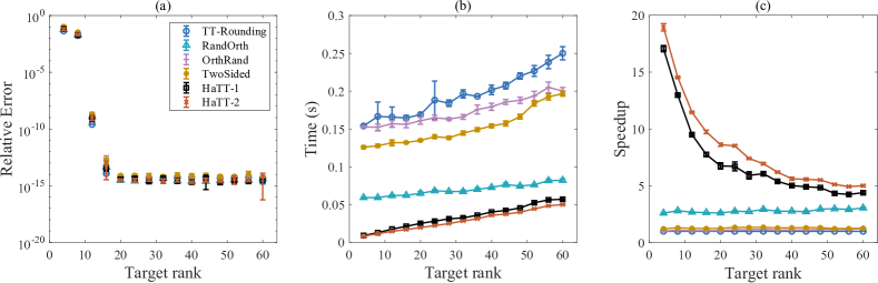
Figure 6: (a) Relative errors, (b) running times, and (c) speedups for Example 1.

We report the relative errors, running times, and speedups (compared to the TT-Rounding algorithm) for all TT recompression algorithms in Fig. 6. As shown in Fig. 6(a), the relative errors obtained by HaTT are comparable to those of other baseline methods, validating the accuracy of HaTT. From Fig. 6(b), we observe that the randomized algorithms are faster than TT-Rounding, and HaTT is particularly effective due to the Hadamard avoiding technique. It follows from Fig. 6(c) that the speedup of HaTT compared to other baseline methods decreases as the target TT rank $\ell$ increases. For this example, the speedup of HaTT compared to TT-Rounding, RandOrth, OrthRand, and TwoSided ranges from $4.2\times\sim 18.9\times$, $1.4\times$ to $7.3\times$, $2.0\times$ to $12.5\times$, and $2.0\times$ to $9.2\times$, respectively.

4.2 Example 2: Hadamard product of random TT tensors with different TT ranks

In this example, we study the performance of HaTT for the Hadamard product of TT tensors with different ranks. Two $7$th-order TT tensors $\bm{\mathcal{Y}},\bm{\mathcal{Z}}\in\mathbb{R}^{20\times 20\times\ldots\times 20}$ are set as random uniform TT tensors (see Definition 1). The corresponding maximal TT rank $r$ or $s$ increases from 60 to 150 in steps of 10. The target TT rank $\ell$ is fixed to $60$. The relative errors, running times, and speedups for all TT recompression algorithms are shown in Fig. 7. According to Fig. 7(a), the accuracy of HaTT is almost the same as RandOrth and OrthRand, though slightly larger than the accuracy of TT-Rounding. As $r$ or $s$ increases, the speedup of HaTT compared to other baseline methods increases rapidly. For $r=s=110$, the HaTT can achieve $5.4\times\sim 115.1\times$ speedup. It should be noted that simulations for $r$ or $s$ larger than $110$ using the baseline methods could not be performed due to memory limitations. Since HaTT avoids explicit representation of the Hadamard product $\bm{\mathcal{Y}}\odot\bm{\mathcal{Z}}$, it can recompress the Hadamard product even when $r=s=150$. This observation fully demonstrates the advantage of HaTT in terms of memory efficiency.

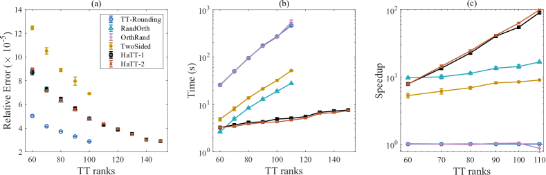
Figure 7: (a) Relative errors, (b) running times, and (c) speedups for Example 2.

4.3 Example 3: application of HaTT in power iteration

We discuss the performance of HaTT in power iteration, which is applied to find the largest element of a TT tensor $\bm{\mathcal{Y}}$ [9]. We generate the tensor $\bm{\mathcal{Y}}$ using a multivariate function, i.e., Qing or Alpine [16, Func. 98 and 6]

$$\text{Qing function:}\ \ f(x_{1},\dots,x_{d}) =\sum_{i=1}^{d}(x_{i}-i)^{2},\ x_{i}\in[-500,500],$$

$$\text{Alpine function:}\ \ f(x_{1},\dots,x_{d}) =\sum_{i=1}^{d}|x_{i}\sin(x_{i})+0.1x_{i}|,\ x_{i}\in[-2.5\pi,2.5\pi],$$

where $d=10,\,20,\,\ldots$, or $50$ is the dimension. The function is discretized on a uniform grid with $10^{d}$ mesh points, resulting in tensor $\bm{\mathcal{Y}}\in\mathbb{R}^{10\times 10\times\cdots\times 10}$. Since the functions are summations of $d$ separable multivariate functions, the tensor $\bm{\mathcal{Y}}$ can be represented as TT tensors with TT ranks $\{1,d,\dots,d,1\}$. In the power iteration, the initial value is set to a tensor whose elements are all $1$, and the maximum number of iterations is set to $100$. We set the target TT rank $\ell$ to $5$ in all TT recompression algorithms. The relative errors of the largest elements obtained by the power iteration equipped with different recompression algorithms are displayed in Fig. 8 (a) and (d), which indicates that the accuracy of the power iteration equipped with any recompression algorithm is acceptable. As shown in Fig. 8 (b–c) and (e–f), the power iteration equipped with HaTT is much faster than other baseline methods, especially for larger $d$.

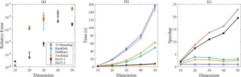
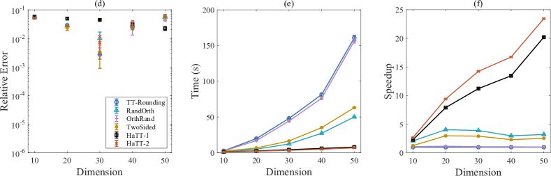
Figure 8: Example 3: power iteration equipped with different recompression algorithms for Qing (above) and Alpine (below) functions.

5 Conclusions and limitations

We propose a Hadamard product-free TT recompression algorithm, named HaTT, for efficiently recompressing the Hadamard product of TT tensors. Utilizing the property of multiplication within the Hadamard product, the HaTT algorithm avoids the explicit representation of the Hadamard product and significantly reduces the overall computational cost of the rounding procedure compared to all existing TT recompression algorithms. Future work will focus on further analysis of the HaTT algorithm and its potential application in recompressing the Hadamard product of quantum TT tensors. Furthermore, this work primarily focuses on recompression when the target ranks are predetermined. Future research will explore tolerance-controlled recompression of the Hadamard product, which is also of significant interest.

Appendix A TT-Rounding

The basic operations of TT tensors usually lead to excessive growth of TT ranks [22]. To suppress it, several recompression algorithms were proposed. The most popular recompression algorithm for TT tensors is TT-Rounding [22]. The TT-Rounding algorithm consists of two steps: orthogonalization and recompression (typically using SVD or truncated SVD). During the orthogonalization step, TT cores are adjusted to satisfy left orthogonality, except for the first TT core $\bm{\mathcal{T}}_{\bm{\mathcal{X}},1}$, using QR decomposition. Subsequently, the TT cores of the approximate tensor are constructed sequentially through the truncated SVD step. The computational procedure of TT-Rounding is detailed in Algorithm 3.

Algorithm 3 TT-Rounding [22]

A $d$th-order TT tensor $\bm{\mathcal{A}}$, target TT ranks $\{\ell_{k}\}_{k=0}^{d}$. TT tensor $\bm{\mathcal{B}}$with TT ranks $\{\ell_{k}\}_{k=0}^{d}$.

1: $\bm{\mathcal{B}}$ = TT-Rounding($\bm{\mathcal{A}}$, $\{\ell_{k}\}_{k=0}^{d}$) Right-to-left orthogonalization

2:     Set $\bm{\mathcal{T}}_{\bm{\mathcal{B}},d}=\bm{\mathcal{T}}_{\bm{\mathcal{A}},d}$. $k=d$ down to 2

3:     $[\HT{\bm{\mathcal{T}}_{\bm{\mathcal{B}},k}}^{\mathsf{T}},\bm{R}]=\text{QR}(\HT{\bm{\mathcal{T}}_{\bm{\mathcal{B}},k}}^{\mathsf{T}})$. $\triangleright$ LQ factorization of $\HT{\bm{\mathcal{T}}_{\bm{\mathcal{B}},k}}$

4:     $\VT{\bm{\mathcal{T}}_{\bm{\mathcal{B}},k-1}}=\VT{\bm{\mathcal{T}}_{\bm{\mathcal{A}},k-1}}\bm{R}^{\mathsf{T}}$.

5:     Set $\bm{\mathcal{T}}_{\bm{\mathcal{B}},1}=\bm{\mathcal{T}}_{\bm{\mathcal{A}},1}$. $k=1$ to $d-1$

6:     $[\VT{\bm{\mathcal{T}}_{\bm{\mathcal{B}},k}},\bm{R}]=\text{QR}(\VT{\bm{\mathcal{T}}_{\bm{\mathcal{B}},k}})$. $\triangleright$ thin QR factorization

7:     $[\hat{\bm{U}},\hat{\bm{\Sigma}},\hat{\bm{V}}]=\text{trucated SVD}(\bm{R},\ell_{k+1})$.

8:     $\VT{\bm{\mathcal{T}}_{\bm{\mathcal{B}},k}}=\VT{\bm{\mathcal{T}}_{\bm{\mathcal{B}},k}}\hat{\bm{U}}$. $\triangleright$ the U matrix to left: $\bm{\mathcal{T}}_{\bm{\mathcal{B}},k}\times^{1}\hat{\bm{U}}$.

9:     $\HT{\bm{\mathcal{T}}_{\bm{\mathcal{B}},k+1}}=\hat{\bm{\Sigma}}\hat{\bm{V}}^{\mathsf{T}}\HT{\bm{\mathcal{T}}_{\bm{\mathcal{A}},k+1}}$. $\triangleright$ the other to right: $\bm{\mathcal{T}}_{\bm{\mathcal{B}},k+1}=\hat{\bm{\Sigma}}\hat{\bm{V}}^{\mathsf{T}}\times^{1}\bm{\mathcal{T}}_{\bm{\mathcal{A}},k+1}$

10: 

Appendix B Random TT tensor

Definition 1 (Random TT tensor).

Given a set of target TT ranks $\{\ell_{k}\}_{k=0}^{d}$, we generate a random Gaussian TT tensor $\bm{\mathcal{R}}\in\mathbb{R}^{n_{1}\times\dots\times n_{d}}$ such that each core tensor $\bm{\mathcal{T}}_{\bm{\mathcal{R}},k}\in\mathbb{R}^{\ell_{k-1}\times n_{k}\times\ell_{k}}$ is filled with random, independent, normally distributed entries with mean $0$ and variance $1/(\ell_{k-1}n_{k}\ell_{k})$ for $1\leq k\leq d$. If each core is filled with random, independent, uniformly distributed entries from $[0,1]$, we call it a random uniform TT tensor.

Appendix C RandOrth

Randomized TT recompression algorithms are inspired by randomized SVD. Consider a matrix $\bm{A}=\bm{B}\bm{C}$, where $\bm{A}\in\mathbb{R}^{m\times n}$, $\bm{B}\in\mathbb{R}^{m\times R}$, $\bm{C}\in\mathbb{R}^{R\times n}$ with $R>\operatorname{rank}(\bm{A})$. The goal of randomized SVD is to find an approximation of $\bm{A}$ with a target rank $\ell<R$. To achieve this, we first generate a random matrix $\bm{\Omega}\in\mathbb{R}^{m\times\ell}$, whose elements are independently drawn from the standard normal distribution. And then we compute the QR factorization of

$$\bm{A}\bm{\Omega}=\bm{B}\bm{C}\bm{\Omega}:=\bm{B}\bm{W}=\bm{Q}\bm{R},$$

where $\bm{Q}\in\mathbb{R}^{m\times\ell}$ has orthogonal columns. We have $\operatorname{range}\bm{Q}\approx\operatorname{range}(\bm{A})$ and use $\bm{Q}(\bm{Q}^{\mathsf{T}}\bm{A})$ to approximate $\bm{A}$, whose accuracy strongly depends on the singular value distribution of $\bm{A}$ [12].

For a TT tensor $\bm{\mathcal{T}}_{\bm{\mathcal{A}},k:d}$, we rewrite it as two TT tensors multiplication: $\bm{\mathcal{T}}_{\bm{\mathcal{A}},k}\times^{1}\bm{\mathcal{T}}_{\bm{\mathcal{A}},(k+1):d}$. Similar to randomized SVD, we multiply a random tensor $\bm{\mathcal{R}}^{(k)}\in\mathbb{R}^{n_{k+1}\times n_{k+2}\times\dots\times n_{d}\times\ell_{k}}$ on the right-hand side to generate a sketch, i.e.,

$$\bm{W}^{(k)}=\bm{\mathcal{T}}_{\bm{\mathcal{A}},(k+1):d}\times^{1,2,\dots,d-k}\bm{\mathcal{R}}^{(k)}\in\mathbb{R}^{r_{k}s_{k}\times\ell_{k}},$$

If $\bm{\mathcal{R}}^{(k)}$ is a sub-tensor of a random Gaussian TT tensor $\bm{\mathcal{R}}$, i.e.,

$$\bm{\mathcal{R}}^{(k)}=\bm{\mathcal{T}}_{\bm{\mathcal{R}},k+1}\times^{1}\bm{\mathcal{T}}_{\bm{\mathcal{R}},k+2}\times^{1}\dots\times^{1}\bm{\mathcal{T}}_{\bm{\mathcal{R}},d},$$

then the corresponding randomized TT recompression algorithm is RandOrth proposed in [2], see Algorithm 4.

Algorithm 4 RandOrth: Randomize-then-Orthogonalize [2]

A TT tensor $\bm{\mathcal{A}}$with ranks $\{r_{k}\}_{k=0}^{d}$, target TT ranks $\{\ell_{k}\}_{k=0}^{d}$A TT tensor $\bm{\mathcal{B}}$with ranks $\{\ell_{k}\}_{k=0}^{d}$

1: $\bm{\mathcal{B}}$ = RandOrth($\bm{\mathcal{A}}$, $\{\ell_{k}\}_{k=0}^{d}$)

2:     Select a random Gaussian TT tensor $\bm{\mathcal{R}}$ with target TT ranks $\{\ell_{k}\}_{k=0}^{d}$

3:     $\bm{W}^{(d-1)}=\HT{\bm{\mathcal{T}}_{\bm{\mathcal{A}},d}}\left(\HT{\bm{\mathcal{T}}_{\bm{\mathcal{R}},d}}\right)^{\mathsf{T}}$ $k=d-1$ down to $2$

4:     $\VT{\bm{\mathcal{T}}_{\bm{\mathcal{Z}},k}}=\VT{\bm{\mathcal{T}}_{\bm{\mathcal{A}},k}}\bm{W}^{(k)}$

5:     $\bm{W}^{(k-1)}=\HT{\bm{\mathcal{T}}_{\bm{\mathcal{Z}},k}}\left(\HT{\bm{\mathcal{T}}_{\bm{\mathcal{R}},k}}\right)^{\mathsf{T}}$

6:     $\bm{\mathcal{T}}_{\bm{\mathcal{B}},1}=\bm{\mathcal{T}}_{\bm{\mathcal{A}},1}$ $k=1$ to $d-1$

7:     $\bm{B}^{(k)}=\VT{\bm{\mathcal{T}}_{\bm{\mathcal{B}},k}}$

8:     $[\VT{\bm{\mathcal{T}}_{\bm{\mathcal{B}},k}},\sim]=\text{QR}(\bm{B}^{(k)}\bm{W}^{(k)})$

9:     $\bm{M}^{(k)}=\left(\VT{\bm{\mathcal{T}}_{\bm{\mathcal{B}},k}}\right)^{\mathsf{T}}\bm{B}^{(k)}$

10:     $\HT{\bm{\mathcal{T}}_{\bm{\mathcal{B}},k+1}}=\bm{M}^{(k)}\HT{\bm{\mathcal{T}}_{\bm{\mathcal{A}},k+1}}$

11: 

Appendix D Two implementation versions of HPCRL

We mentioned two ways to get the rank-1 decomposition of $\bm{W}^{(k)}$ in Subsection 3.1. We denote the one with (truncated) SVD (5) HPCRL-1 and the one with direct representation (6). We show the algorithm of both methods in Algorithm 5 and 6, respectively.

Algorithm 5 HPCRL-1: Generate partial contractions $\{\bm{W}^{(k)}\}_{k=1}^{d-1}$ of the Hadamard product with truncated SVD

Two TT tensors $\bm{\mathcal{Y}}$and $\bm{\mathcal{Z}}$, whose Hadamard product $\bm{\mathcal{Y}}\odot\bm{\mathcal{Z}}$needs to be recompressed. A randomized Gaussian TT tensor $\bm{\mathcal{R}}$. A set of sketch matrices $\{\bm{W}^{(k)}\}_{k=1}^{d-1}$.

1: $\{\bm{W}^{(k)}\}_{k=1}^{d-1}$ = HPCRL-1($\bm{\mathcal{Y}}$, $\bm{\mathcal{Z}}$, $\bm{\mathcal{R}}$)

2:     $\bm{W}^{(d-1)}=\HT{\bm{\mathcal{T}}_{\bm{\mathcal{Y}},d}\boxtimes^{1}\bm{\mathcal{T}}_{\bm{\mathcal{Z}},d}}\HT{\bm{\mathcal{T}}_{\bm{\mathcal{R}},d}}^{\mathsf{T}}$ $k=d-1$ down to $2$ (truncated) SVD and then truncate

3:     $\bm{W}^{(k)}=\sum_{\gamma=1}^{R}\sigma^{(k)}_{\gamma}\bm{U}^{(k)}(:,{\gamma})\bm{V}^{(k)}(:,{\gamma})^{\mathsf{T}}:=\bm{U}^{(k)}\bm{S}^{(k)}(\bm{V}^{(k)})^{\mathsf{T}}$ $i_{k}=1$ to $n_{k}$ $\gamma=1$ to $R$

4:     $\bm{U}^{(k)}_{\gamma}=\bm{U}^{(k)}(:,\gamma)\big{|}^{s_{k}}_{r_{k}}$

5:     $\bm{W}_{L}(:,\overline{i_{k}\gamma})=\text{vec}\big{(}\bm{\mathcal{T}}_{\bm{\mathcal{Z}},k}(i_{k})\bm{U}^{(k)}_{\gamma}(\bm{\mathcal{T}}_{\bm{\mathcal{Y}},k}(i_{k}))^{\mathsf{T}}\big{)}$ $\triangleright$ $\mathbb{R}^{s\times s}\times\mathbb{R}^{s\times r}\times\mathbb{R}^{r\times r}$

6:     $\bm{W}_{R}(:,\overline{i_{k}\gamma})=\bm{\mathcal{T}}_{\bm{\mathcal{R}},k}(i_{k})\bm{V}^{(k)}(:,\gamma)$ $\triangleright$ $\mathbb{R}^{\ell\times\ell}\times\mathbb{R}^{\ell}$

7:     $\bm{W}^{(k-1)}=\bm{W}_{L}(\bm{I}_{n_{k}}\otimes\bm{S}^{(k}))\bm{W}_{R}^{\mathsf{T}}$ $\triangleright$ $\mathbb{R}^{rs\times nR}\times\mathbb{R}^{nR\times nR}\text{(diagonal)}\times\mathbb{R}^{nR\times\ell}$

8: 

Algorithm 6 HPCRL-2: Generate partial contractions $\{\bm{W}^{(k)}\}_{k=1}^{d-1}$ of the Hadamard product with direct representation

Two TT tensors $\bm{\mathcal{Y}}$and $\bm{\mathcal{Z}}$, whose Hadamard product $\bm{\mathcal{Y}}\odot\bm{\mathcal{Z}}$needs to be recompressed. A randomized Gaussian TT tensor $\bm{\mathcal{R}}$. A set of sketch matrices $\{\bm{W}^{(k)}\}_{k=1}^{d-1}$.

1: $\{\bm{W}^{(k)}\}_{k=1}^{d-1}$ = HPCRL-2($\bm{\mathcal{Y}}$, $\bm{\mathcal{Z}}$, $\bm{\mathcal{R}}$)

2:     $\bm{W}^{(d-1)}=\HT{\bm{\mathcal{T}}_{\bm{\mathcal{Y}},d}\boxtimes^{1}\bm{\mathcal{T}}_{\bm{\mathcal{Z}},d}}\HT{\bm{\mathcal{T}}_{\bm{\mathcal{R}},d}}^{\mathsf{T}}$ $k=d-1$ down to $2$ $i_{k}=1$ to $n_{k}$

3:     $\bm{W}_{R}(:,((i_{k}-1)\ell_{k}+1):i_{k}\ell_{k})=\bm{\mathcal{T}}_{\bm{\mathcal{R}},k}(i_{k})$ $\gamma=1$ to $\ell_{k}$

4:     $\bm{W}^{(k)}_{\gamma}=\bm{W}^{(k)}(:,\gamma)\big{|}^{s_{k}}_{r_{k}}$

5:     $\bm{W}_{L}(:,\overline{i_{k}\gamma})=\text{vec}\big{(}\bm{\mathcal{T}}_{\bm{\mathcal{Z}},k}(i_{k})\bm{W}^{(k)}_{\gamma}(\bm{\mathcal{T}}_{\bm{\mathcal{Y}},k}(i_{k}))^{\mathsf{T}}\big{)}$ $\triangleright$ $\mathbb{R}^{s\times s}\times\mathbb{R}^{s\times r}\times\mathbb{R}^{r\times r}$

6:     $\bm{W}^{(k-1)}=\bm{W}_{L}\bm{W}_{R}^{\mathsf{T}}$$\triangleright$ $\mathbb{R}^{rs\times n\ell}\times\mathbb{R}^{n\ell\times\ell}$

7: 

Appendix E Complexity analysis

We first introduce the complexity of the relevant operations. For $\bm{X}\in\mathbb{R}^{m\times n}$ with $m>n$, the econ-QR decomposition of $\bm{X}$ is denoted by $\bm{X}=\bm{Q}\bm{R}$, where $\bm{Q}\in\mathbb{R}^{m\times n}$ has orthonormal columns and $\bm{R}\in\mathbb{R}^{n\times n}$ is upper triangular. The econ-QR decomposition can be implemented by the Householder algorithm [11], which costs $4mn^{2}-4n^{3}/3$ if we only require $\bm{Q}$. We denote the reduced SVD of $\bm{X}$ as $\bm{X}=\bm{U}\bm{S}\bm{V}^{\mathsf{T}}$, where $\bm{U}\in\mathbb{R}^{m\times n}$ and $\bm{V}\in\mathbb{R}^{n\times n}$ have orthonormal columns, and $\bm{S}\in\mathbb{R}^{n\times n}$ is diagonal matrix. According to [11], it costs $O(mn^{2})$ flops. In addition, the flop efficiency of matrix-matrix multiplication between $\bm{X}\in\mathbb{R}^{m\times n}$ and $\bm{Y}\in\mathbb{R}^{n\times r}$ is $m(2n-1)r$. For convenience of description, we assume that the TT ranks of $\bm{\mathcal{Y}}$, $\bm{\mathcal{Z}}$, and $\bm{\mathcal{R}}$ are $\{1,r,r,\ldots,r,1\}$, $\{1,s,s,\ldots,s,1\}$, and $\{1,\ell,\ell,\ldots,\ell,1\}$, respectively. Under this assumption, the sketching matrices $\{\bm{W}^{(k)}\}_{k=1}^{d-1}$ have the size of $\mathbb{R}^{rs\times\ell}$ and rank of $R$. Moreover, we always assume that $\ell<rs$.

E.1 Complexity of HPCRL

Complexity of HPCRL-1.

1. The flops of (truncated) SVD: $O((d-2)\cdot rs\ell^{2})$.

2. The flops of construction $\bm{W}_{L}$: $(d-2)n\cdot rsR(2r+2s-2)$.

3. The flops of construction $\bm{W}_{R}$: $(d-2)n\cdot R\ell(2\ell-1)$.

4. The flops of $\bm{W}_{L}(\bm{I}_{n_{k}}\otimes\bm{S})\bm{W}_{R}^{\mathsf{T}}$: $(d-2)\cdot(nR\ell+2nrsR\ell-rs\ell)$.

5. Total flops of HPCRL-1: $(d-2)[nR(2r^{2}s+2s^{2}r+2rs\ell)+O(rs\ell^{2})]$.

6. Memory requirement for $\bm{W}^{(k)}$: $(d-1)rs\ell$.

7. Memory requirement for $\bm{U}^{(k)}$, $\bm{S}^{(k)}$, and $\bm{V}^{(k)}$: $rsR+R\ell+R$.

8. Memory requirement for $\bm{W}_{L}$ and $\bm{W}_{R}$ (can be further avoided): $nrsR+nR\ell$.

Complexity of HPCRL-2.

1. The flops of direct representation (6): 0.

2. The flops of construction $\bm{W}_{L}$: $(d-2)n\cdot rs\ell(2r+2s-2)$.

3. The flops of construction $\bm{W}_{R}$: 0.

4. $\bm{W}_{L}\bm{W}_{R}^{\mathsf{T}}$: $(d-2)rs\ell(2n\ell-1)$.

5. Total flops of HPCRL-2: $(d-2)\cdot[n\cdot rs\ell(2r+2s+2\ell)]$.

6. Memory requirement for $\bm{W}^{(k)}$: $(d-1)rs\ell$.

7. Memory requirement for $\bm{U}^{(k)}$, $\bm{S}^{(k)}$, and $\bm{V}^{(k)}$: 0.

8. Memory requirement for $\bm{W}_{L}$ and $\bm{W}_{R}$ (can be further avoided): $rsn\ell$.

E.2 Complexity of HaTT

Complexity of HaTT-1.

1. The flops of HPCRL-1: $(d-2)[nR(2r^{2}s+2s^{2}r+2rs\ell)+O(rs\ell^{2})]$.

2. The flops of multiplication: $\bm{X}^{(k)}$ and $\bm{W}^{(k)}$: $(d-1)n\ell^{2}(2rs-1)$.

3. The flops of econ-QR $\bm{X}^{(k)}\bm{W}^{(k)}$: $(d-1)(4n-4/3)\ell^{3}$.

4. The flops of $\bm{M}^{(k)}=(\bm{Q}^{(k)})^{\mathsf{T}}\bm{X}^{(k)}$: $(d-1)rs\ell(2\ell n-1)$.

5. Updating $\bm{\mathcal{T}}_{\bm{\mathcal{X}},k+1}$ by (9): $(d-1)nrs\ell(2r+2s-2)$.

6. Total flops of HaTT-1: $(d-2)[rsn\hat{R}(4r+4s+4\ell+2\ell^{2}/\hat{R})+O(rs\ell^{2})]$, where $\hat{R}=\frac{R+\ell}{2}$.

7. Memory requirement for all TT cores of $\bm{\mathcal{X}}$, $\bm{\mathcal{Y}}$ and $\bm{\mathcal{Z}}$: $dn(r^{2}+s^{2}+\ell^{2})$

8. Memory requirement for $\bm{X}^{(k)}$: $rsn\ell$.

9. Memory requirement for $\bm{Q}^{(k)}$ (we save $\bm{Q}^{(k)}$ in $\bm{\mathcal{T}}_{\bm{\mathcal{X}},k}$), and $\bm{M}^{(k)}$: $rs\ell$.

10. Memory requirement for $\bm{\mathcal{T}}_{\bm{\mathcal{X}},k+1}$ (we save the temporary updated $\bm{\mathcal{T}}_{\bm{\mathcal{X}},k+1}$ in the space of $\bm{X}^{(k)}$): $0$.

Complexity of HaTT-2.

1. The flops of HPCRL-2: $(d-2)\cdot[nrs\ell(2r+2s+2\ell)]$.

2. The flops of multiplication: $\bm{X}^{(k)}$ and $\bm{W}^{(k)}$: $(d-1)n\ell^{2}(2rs-1)$.

3. The flops of econ-QR $\bm{X}^{(k)}\bm{W}^{(k)}$: $(d-1)(4n-4/3)\ell^{3}$.

4. The flops of $\bm{M}^{(k)}=(\bm{Q}^{(k)})^{\mathsf{T}}\bm{X}^{(k)}$: $(d-1)rs\ell(2\ell n-1)$.

5. Updating $\bm{\mathcal{T}}_{\bm{\mathcal{X}},k+1}$ by (9): $(d-1)nrs\ell(2r+2s-2)$.

6. Total flops of HaTT-2: $(d-2)[nrs\ell(4r+4s+6\ell)].$

7. Memory requirement for all TT cores of $\bm{\mathcal{X}}$, $\bm{\mathcal{Y}}$ and $\bm{\mathcal{Z}}$: $dn(r^{2}+s^{2}+\ell^{2})$

8. Memory requirement for $\bm{X}^{(k)}$: $rsn\ell$.

9. Memory requirement for $\bm{Q}^{(k)}$ (we save $\bm{Q}^{(k)}$ in $\bm{\mathcal{T}}_{\bm{\mathcal{X}},k}$), and $\bm{M}^{(k)}$: $rs\ell$.

10. Memory requirement for $\bm{\mathcal{T}}_{\bm{\mathcal{X}},k+1}$ (we save the temporary updated $\bm{\mathcal{T}}_{\bm{\mathcal{X}},k+1}$ in the space of $\bm{X}^{(k)}$): $0$.

E.3 Comparison of complexity for different TT recompression algorithms

We summarize the flops of partial contraction and recompression for the Hadamard product $\bm{\mathcal{Y}}\odot\bm{\mathcal{Z}}$ with different algorithms in Table 2.

Table 2: Flops when computing the Hadamard product of two TT tensors.

Algorithms	Computational cost (flops)
PartialContractionRL	$(d-2)n(2rs\ell^{2}+2r^{2}s^{2}\ell)$
HPCRL-1	$(d-2)[nR(2r^{2}s+2s^{2}r+2rs\ell+2\ell^{2}-2rs)-rs\ell+O(rs\ell^{2})]$
HPCRL-2	$(d-2)[n\ell(2r^{2}s+2s^{2}r+2rs\ell+\ell-2rs)-rs\ell]$
TT-Rounding	$(d-2)n(5r^{3}s^{3}+6r^{2}s^{2}\ell+2rs\ell^{2})$
OrthRand	$(d-2)n(5r^{3}s^{3}+2r^{2}s^{2}\ell+4rs\ell^{2})$
RandOrth	$(d-2)n(4r^{2}s^{2}\ell+6rs\ell^{2})$
TwoSided	$(d-2)n(6r^{2}s^{2}\ell+6rs\ell^{2})$
HaTT-1	$(d-2)[nrs\hat{R}(4r+4s+4\ell+2\ell^{2}/\hat{R})+O(rs\ell^{2})]$
HaTT-2	$(d-2)[nrs\ell(4r+4s+6\ell)]$

Appendix F The definition of relative error

The relative error of a TT recompression algorithm is defined as

$$\|\bm{\mathcal{A}}^{\mathit{round}}-\bm{\mathcal{A}}\|_{\mathrm{F}}/\left\|\bm{\mathcal{A}}\right\|_{\mathrm{F}},$$

where $\bm{\mathcal{A}}^{\mathit{round}}$ is the low rank TT tensor obtained by TT recompression algorithm and $\bm{\mathcal{A}}$ is the exact solution of $\bm{\mathcal{Y}}\odot\bm{\mathcal{Z}}$.

For power iteration, the relative error is defined as:

$$|M-M^{\mathit{real}}|/M^{\mathit{real}},$$

where $M$ is the result of power iteration and $M^{\mathit{real}}$ is the exact solution.

Appendix G Comparison between HaTT-1 and HaTT-2

According to the complexity analysis given in Appendix E, HaTT-1 is more efficient than HaTT-2 for $R\ll\ell$. However, numerical results reported in Section 4 show that HaTT-1 is slightly slower than HaTT-2. In this section, we introduce an example to compare HaTT-1 and HaTT-2, in which $R\ll\ell$. Let $\bm{\mathcal{Y}}\in\mathbb{R}^{20\times\dots\times 20}$ be a $7$th order Hilbert-type TT tensor with ranks $\{1,100,\dots,100,1\}$. The elements of the $k$th TT core of $\bm{\mathcal{Y}}$ are defined as

$$\bm{\mathcal{T}}_{\bm{\mathcal{Y}},k}(\alpha_{k-1},i_{k},\alpha_{k})=\frac{1}{\alpha_{k-1}+i_{k}+\alpha_{k}-1},\quad 1\leq\alpha_{k-1}\leq r_{k-1},1\leq i_{k}\leq n_{k},1\leq\alpha_{k}\leq r_{k}.$$

HaTT-1 and HaTT-2 are then used to recompress the Hadamard product $\bm{\mathcal{A}}=\bm{\mathcal{Y}}\odot\bm{\mathcal{Y}}$. Due to the rapid decay of singular values of $\bm{W}^{(k)}$, we employ a truncated SVD in HaTT-1, limiting the decomposition to a maximum of 5 singular values. The target rank is set as $\ell=30,40,\ldots,120$. The relative errors for HaTT-1 and HaTT-2 are displayed in Fig. 9(a), showing that the errors are almost the same for both methods. The computing times for the two methods are given in Fig. 9(b), which demonstrates that HaTT-1 outperforms HaTT-2 for $\ell>60$. This observation is consistent with the complexity analysis.

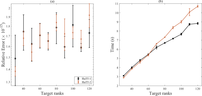
Figure 9: Comparasion of HaTT-1 and HaTT-2 when $\bm{W}^{(k)}$ has a low rank approximation.

References

- Al Daas et al. [2022] Hussam Al Daas, Grey Ballard, and Lawton Manning. Parallel tensor train rounding using Gram SVD. In 2022 IEEE International Parallel and Distributed Processing Symposium (IPDPS), pages 930–940. IEEE, 2022.
- Al Daas et al. [2023] Hussam Al Daas, Grey Ballard, Paul Cazeaux, Eric Hallman, Agnieszka Międlar, Mirjeta Pasha, Tim W Reid, and Arvind K Saibaba. Randomized algorithms for rounding in the tensor-train format. SIAM Journal on Scientific Computing, 45(1):A74–A95, 2023.
- Bonizzoni et al. [2016] Francesca Bonizzoni, Fabio Nobile, and Daniel Kressner. Tensor train approximation of moment equations for elliptic equations with lognormal coefficient. Computer Methods in Applied Mechanics and Engineering, 308:349–376, 2016.
- Cichocki et al. [2016] Andrzej Cichocki, Namgil Lee, Ivan Oseledets, Anh-Huy Phan, Qibin Zhao, Danilo P Mandic, et al. Tensor networks for dimensionality reduction and large-scale optimization: Part 1 low-rank tensor decompositions. Foundations and Trends® in Machine Learning, 9(4-5):249–429, 2016.
- Cichocki et al. [2017] Andrzej Cichocki, Anh-Huy Phan, Qibin Zhao, Namgil Lee, Ivan Oseledets, Masashi Sugiyama, Danilo P Mandic, et al. Tensor networks for dimensionality reduction and large-scale optimization: Part 2 applications and future perspectives. Foundations and Trends® in Machine Learning, 9(6):431–673, 2017.
- Daas et al. [2022] Hussam Al Daas, Grey Ballard, and Peter Benner. Parallel algorithms for tensor train arithmetic. SIAM Journal on Scientific Computing, 44(1):C25–C53, 2022.
- Dolgov et al. [2015] Sergey Dolgov, Boris N Khoromskij, Alexander Litvinenko, and Hermann G Matthies. Polynomial chaos expansion of random coefficients and the solution of stochastic partial differential equations in the tensor train format. SIAM/ASA Journal on Uncertainty Quantification, 3(1):1109–1135, 2015.
- Doostan and Iaccarino [2009] Alireza Doostan and Gianluca Iaccarino. A least-squares approximation of partial differential equations with high-dimensional random inputs. Journal of Computational Physics, 228(12):4332–4345, 2009.
- Espig et al. [2020] Mike Espig, Wolfgang Hackbusch, Alexander Litvinenko, Hermann G Matthies, and Elmar Zander. Iterative algorithms for the post-processing of high-dimensional data. Journal of Computational Physics, 410:109396, 2020.
- Ganahl et al. [2017] Martin Ganahl, Julián Rincón, and Guifre Vidal. Continuous matrix product states for quantum fields: An energy minimization algorithm. Physical Review Letters, 118(22):220402, 2017.
- Golub and Van Loan [2013] Gene H Golub and Charles F Van Loan. Matrix computations. JHU press, 2013.
- Halko et al. [2011] Nathan Halko, Per-Gunnar Martinsson, and Joel A Tropp. Finding structure with randomness: Probabilistic algorithms for constructing approximate matrix decompositions. SIAM review, 53(2):217–288, 2011.
- Han et al. [2018] Zhao-Yu Han, Jun Wang, Heng Fan, Lei Wang, and Pan Zhang. Unsupervised generative modeling using matrix product states. Physical Review X, 8(3):031012, 2018.
- Holtz et al. [2012] Sebastian Holtz, Thorsten Rohwedder, and Reinhold Schneider. The alternating linear scheme for tensor optimization in the tensor train format. SIAM Journal on Scientific Computing, 34(2):A683–A713, 2012.
- Iaconis et al. [2024] Jason Iaconis, Sonika Johri, and Elton Yechao Zhu. Quantum state preparation of normal distributions using matrix product states. npj Quantum Information, 10(1):15, 2024.
- Jamil and Yang [2013] Momin Jamil and Xin-She Yang. A literature survey of benchmark functions for global optimisation problems. International Journal of Mathematical Modelling and Numerical Optimisation, 4(2):150–194, 2013.
- Khoromskij [2018] Boris N Khoromskij. Tensor numerical methods in scientific computing, volume 19. Walter de Gruyter GmbH & Co KG, 2018.
- Kressner and Perisa [2017] Daniel Kressner and Lana Perisa. Recompression of Hadamard products of tensors in Tucker format. SIAM Journal on Scientific Computing, 39(5):A1879–A1902, 2017.
- Lee and Cichocki [2014] Namgil Lee and Andrzej Cichocki. Fundamental tensor operations for large-scale data analysis in tensor train formats. arXiv preprint arXiv:1405.7786, 2014.
- Lee and Cichocki [2018] Namgil Lee and Andrzej Cichocki. Fundamental tensor operations for large-scale data analysis using tensor network formats. Multidimensional Systems and Signal Processing, 29:921–960, 2018.
- Oseledets et al. [2011] IV Oseledets, S Dolgov, et al. MATLAB TT-Toolbox version 2.2. Math Works, Natick, MA, 2011.
- Oseledets [2011] Ivan V Oseledets. Tensor-train decomposition. SIAM Journal on Scientific Computing, 33(5):2295–2317, 2011.
- Richter et al. [2021] Lorenz Richter, Leon Sallandt, and Nikolas Nüsken. Solving high-dimensional parabolic PDEs using the tensor train format. In International Conference on Machine Learning, pages 8998–9009. PMLR, 2021.
- Risthaus and Schneider [2022] Lennart Risthaus and Matti Schneider. Solving phase-field models in the tensor train format to generate microstructures of bicontinuous composites. Applied Numerical Mathematics, 178:262–279, 2022.
- Shi et al. [2023] Tianyi Shi, Maximilian Ruth, and Alex Townsend. Parallel algorithms for computing the tensor-train decomposition. SIAM Journal on Scientific Computing, 45(3):C101–C130, 2023.
- Sidiropoulos et al. [2017] Nicholas D Sidiropoulos, Lieven De Lathauwer, Xiao Fu, Kejun Huang, Evangelos E Papalexakis, and Christos Faloutsos. Tensor decomposition for signal processing and machine learning. IEEE Transactions on signal processing, 65(13):3551–3582, 2017.
- Sozykin et al. [2022] Konstantin Sozykin, Andrei Chertkov, Roman Schutski, Anh-Huy Phan, Andrzej S Cichocki, and Ivan Oseledets. TTOpt: A maximum volume quantized tensor train-based optimization and its application to reinforcement learning. Advances in Neural Information Processing Systems, 35:26052–26065, 2022.
- Su et al. [2020] Jiahao Su, Wonmin Byeon, Jean Kossaifi, Furong Huang, Jan Kautz, and Anima Anandkumar. Convolutional tensor-train LSTM for spatio-temporal learning. Advances in Neural Information Processing Systems, 33:13714–13726, 2020.
- Wang et al. [2017] David S Wang, Charles D Hill, and Lloyd CL Hollenberg. Simulations of Shor’s algorithm using matrix product states. Quantum Information Processing, 16:1–13, 2017.
- Xie et al. [2023] Shiyao Xie, Akinori Miura, and Kenji Ono. Error-bounded scalable parallel tensor train decomposition. In 2023 IEEE International Parallel and Distributed Processing Symposium Workshops (IPDPSW), pages 345–353. IEEE, 2023.
- Yang et al. [2017] Yinchong Yang, Denis Krompass, and Volker Tresp. Tensor-train recurrent neural networks for video classification. In International Conference on Machine Learning, pages 3891–3900. PMLR, 2017.
- Zhou et al. [2020] Yiqing Zhou, E Miles Stoudenmire, and Xavier Waintal. What limits the simulation of quantum computers? Physical Review X, 10(4):041038, 2020.