Statistical Inference for Four-Regime Segmented Regression Models
Abstract
Segmented regression models offer model flexibility and interpretability as compared to the global parametric and the nonparametric models, and yet are challenging in both estimation and inference. We consider a four-regime segmented model for temporally dependent data with segmenting boundaries depending on multivariate covariates with non-diminishing boundary effects. A mixed integer quadratic programming algorithm is formulated to facilitate the least square estimation of the regression and the boundary parameters. The rates of convergence and the asymptotic distributions of the least square estimators are obtained for the regression and the boundary coefficients, respectively. We propose a smoothed regression bootstrap to facilitate inference on the parameters and a model selection procedure to select the most suitable model within the model class with at most four segments. Numerical simulations and a case study on air pollution in Beijing are conducted to demonstrate the proposed approach, which shows that the segmented models with three or four regimes are suitable for the modeling of the meteorological effects on the PM2.5 concentration.
keywords:
[class=MSC]keywords:
and
1 Introduction
Regression analysis is a pivotal tool in modeling the relationship between dependent and independent variables and for prediction purposes. It is often conducted via two types of models: the global parametric and local nonparametric models. The global parametric models, such as the linear and polynomial regression models, have the advantages of interpretability and computation simplicity. However, they often perform poorly due to model misspecification as the underlying model may change over different parts of the domain. To have better adaptability, nonparametric local models facilitated by the kernel smoothing, the wavelets or splines, or the regression trees, have been introduced. The local model’s complexities increase with the data’s dimension and the sample sizes, elevating the risk of overfitting. The segmented model is a compromise between the global and the local models as they are as interpretable as the global parametric models but have improved model specifications.
Conventional threshold regression model (also called regime switching model) [32] was the first generation of the segmented models. It assumes that the regression function is of form , where is an observable scalar variable that can be either a time index or a pre-specified random variable. The threshold regression model has a wide range of applications in empirical research, ranging from modeling effects of shocks to economic systems over the business cycles [27], the dose-response models in biostatistics [29], and in sociological research [5]. Statistical inference of the threshold regression model with a univariate splitting variable has been well developed. [6], [15] and [16] established asymptotic properties of the least squares estimators of the threshold regression models and proposed tests on the threshold effect. As extensions, [12] and [23] introduced the multiple threshold regression model with splits and regimes (segments) and investigated the statistical inference problems.
A limitation of the existing threshold regression approach is that the splitting threshold is largely determined by a univariate variable . [1] showed difficulties in finding the univariate splitting variable in the analysis of macroeconomic effects of fiscal policies, and [19] indicated that a univariate was not suitable to regulate the gene effects on disease risks as the risk of developing a particular disease was due to multiple genes. Recently, [22] and [35] extended the threshold regression to allow regime switching driven by a multivariate random vector which is either observable or obtained via a factor model. Although these works overcome the limitation of the univariate split variable, the setting of at most two regimes can be restrictive for some applications. Machine learning methods, such as the convex piece-wise linear fitting, can produce segmented linear regression with unlimited number of regimes. However, as these methods were focused on the fitting performances, the underlying segmented models may not be identifiable with the suggested procedures. The finite mixture models (FMM) proposed by [20] can also produce a subgroup linear model fitting for heterogeneous data. However, the subgroups from the FMMs do not lead to parameterized boundaries, and thus are less interpretable than the segmented linear models.
Our study is motivated from modelling the meteorological effects on PM2.5 concentration in Beijing, where a global parametric model is too simple to offer good fitting performances and a nonparametric model may be too local and do not provide sufficient atmospheric interpretation. The air pollution in Beijing is typically governed by different meteorological regimes, namely the removal process by favourable northerly wind which removes PM2.5 to a low level, the calm regime between the northerly cleaning and the start of the transported pollution driven under the southerly wind, the pollution growth regime under southerly wind that transports polluted air from the south, and air stagnation regime after the pollution has peaked, followed by the next removal process by the northerly wind. These motivate the four-regime segmented regression model in this work. As the air quality and meteorological data are time series, we consider temporally dependent data in the study.
Motivated by the air pollution problem, we consider four-regime regression models whose splitting hypersplines are determined by linear combinations of two multivariate covariates and , where the splitting variables and can be any regressors, and the two splitting hyperplanes can intersect. These make the four regime-regression model less restrictive than the multiple threshold regression model of [2] and [23] where the splitting variable is univariate, and hence allows not necessarily parallel boundary hyperplanes. The four-regime models include two and three regime models as special cases, where the splitting boundaries are either parallel or two adjacent regimes share the same regression coefficient and hence can be merged.
The main contributions of the study are the following. We first establish the consistency and the asymptotic distributions of the least squares estimators (LSEs) for both the boundary and the regression coefficients under the four-regime regression model with temporally dependent -mixing observations, overcoming challenges posed by (i) the irregular objective function, (ii) the fixed boundary edge effects rather than the diminishing effects commonly treated in the literature and (iii) the unconventional form of the asymptotic distribution for the boundary coefficient vector. It is found that the asymptotic distribution of LSEs for the boundary coefficients is determined by the minimizers of a compound multivariate Poisson process, whose jumps depend on the points near the true hyperplanes, and the boundary coefficient estimators are asymptotically independent of the regression coefficient estimators.
The generalization to the four regimes with two splitting boundaries brings considerable computational challenges. Although the LSE of the conventional threshold regression can be obtained with the grid search method, it is not practical in our setting as the boundaries are defined with multivariate variables. To overcome the challenges, we draw inspiration from [3] and [22] and propose an algorithm based on the mixed integer quadratic programming (MIQP), which is not only computationally efficient but also can be further accelerated by adding an iterative component. It is shown the algorithm can facilitate efficient computation of the LSEs with the rather non-regular form of the least squares objective function.
To permit statistical inference, especially in light of the rather unusual asymptotic distribution for the boundary coefficient estimates, we develop a smoothed regression bootstrap method and establish its consistency for approximating the distribution of the LSEs. Furthermore, the properties of the LSEs under degenerated segmented models with less than four regimes are investigated. In order to find the right segmented models with up to four segments, we propose a model selection method with a backward elimination procedure that is shown to be able to consistently choose the right number of regimes.
The paper is organized as follows. Section 2 introduces the four-regime regression model. Section 3 presents the theoretical properties and the asymptotic distribution of the LSEs for the regression and boundary parameters. In Section 4, we construct a mixed integer quadratic programming (MIQP) algorithm to efficiently compute the LSEs. Section 5 considers inference problems for the four-regime regression model. Section 6 investigates the properties of the proposed estimator under degenerated models with less than four regimes and proposes a model selection method. Sections 7 and 8 report simulation and empirical results, respectively. Section 9 conclude the paper with possible extensions. All technical proofs are relegated to a supplementary material (SM, [33]).
2 Model setup
We first introduce some notations. We use for the indicator function of an event , for the -norm of vector and for the -neighborhood of . Define as the sub-vector of excluding its first element, i.e., . We use to denote the cardinality of a set . For any two sets and , we denote as their symmetric difference.
Let be a sequence of observations, where is the response variable to covariates and two partitioning variables for and , which determine the boundaries of the segments or regimes. The variables , and can share common variables. The four-regime regression model is
| (2.1) |
where is the union of variables of and , are the regression coefficients, are the boundary coefficients, is the residual satisfying with a finite second moment, and is the -th region split by the hyperplanes for . The overall parameter of interest is where and . We let , and denote the respective true parameters. For any observation , it is the signs of and that determine which regression region it is located at. Denote by and . Then we can write Model (2.1) equivalently as
| (2.2) |
which explicitly reflects the role of in Model (2.1).
Remark 2.1.
Although the splitting hyperplanes appears linear, non-linearity may be accommodated by including nonlinear transformed variables in , for instance, . The same extension can be conducted to . It is also noted that in the special case of having the same distribution with , the four segments under are not distinguishable from that under . Consequently, is only identifiable up to some permutations. To avoid such situation, we assume that the distributions of and are distinct.
Remark 2.2.
Since the signs of and determine the regimes in Model (2.1), and have to be normalized in order to be identifiable. For any candidate of , we normalize it by its first element , resulting in where is assumed to take values in a compact set. As noted in [22], an alternative normalization is . In this study, we employ the former as it has one less parameter.
3 Estimation and asymptotic properties
In this section, we outline the least squares (LS) estimation for of the four-regime regression model, and establish the convergence rates of the LS estimators for the regression coefficient and the boundary coefficient followed by providing their asymptotic distributions.
With the data sample , in view of , we define the following least squares criterion function
| (3.1) |
and the parameter space is , where is a compact set in and the first element of any is normalized as for each , and is a compact set in . Since is strictly convex in and piece-wise constant in with at most jumps, it has a unique minimizer for , but a set of minimizers for , which is denoted as , such that a LSE satisfies
| (3.2) |
It is noted that for any two , the segmented regimes under the corresponding hyperplanes must be the same, as otherwise the estimated regression coefficients will be distinct. In addition, the set is convex since for each or , and imply that for all with . In the rest of this section, we investigate the properties of the LS estimators with .
3.1 Identification and consistency
Here we discuss the identification of and establish the consistency of the LSEs . Let follow the stationary distribution of , and for and to indicate whether is located on the true hyperplane or not. Let be the set consisting of index pairs if and are two adjacent regions split by . Specifically, and according to the provision in the lines above (2.2). Furthermore, let be the union vector of variables in and
Assumption 1 (temporal dependence).
(i) The time series is strictly stationary and -mixing with the mixing coefficient for finite positive constants and , where , where denotes the -filed generated by . (ii) , where is a filtration generated by .
Assumption 2 (identification).
For and , (i) and are not identically distributed. (ii) There exists a such that almost surely for and for any , where is the vector after excluding ’s th element; without loss of generality, assume . (iii) For any and , the smallest eigenvalue of for some constant . (iv) For , for some constant .
Assumption 3.
(i) , and . (ii) For each and , if , for some constants .
Assumption 1 (i) prescribes the strict stationarity and -mixing condition on the time series, as used in the existing time-series threshold regression literature ([16] and [22]). It is noted that such a decaying rate is only required in deriving the limiting distribution of , which can be relaxed to the polynomial decay for Theorem 3.1 and Theorem 3.2. Assumption 1 (ii) imposes a martingale difference condition for the noises, which is standard for time series regressions.
Assumption 2 is for the identification of . Specifically, without Assumption 2 (i), are not distinguishable from as discussed in Remark 2.1. It is noted that the methods and theories in the rest of the papers are applicable without such a condition, while a permutation for and is possibly required. Section F of the SM ([33]) provides sufficient conditions for Assumption 2 (ii), which ensures there are positive probability of observations located around the true splitting hyperplanes. Discrete variables can be accommodated in , as long as it includes at least one continuous variable, say . Otherwise, if all the splitting variables are discretely distributed, then will be piece-wise constant and will not be identifiable. Assumption 2 (iii) guarantees that the splittings by candidate hyperplanes do not lead to degenerated covariance matrices, which is needed for the identification of . Assumption 2 (iv) means that adjacent regimes have distinguishable regression coefficients so that the splitting effect of each hyperplane is strictly bounded away , which is similar to the fixed threshold effect models treated in [6] and [35]. Assumption 3 (i) is a moment condition, and (ii) means is continuous at , implying that is continuous at the true parameter .
The identification of is formally ensured in the following proposition.
The proposition ensures that despite the multiple LS estimates , the underlying is unique. The following theorem shows that any LSE estimators defined in (3.2) are consistent to . It is worth noting that though there exist infinitely many solutions which are collected in the convex set , the consistency of each can be guaranteed, which implies that the solution set is a local neighborhood of with a shrinking radius.
With the estimated splitting hyperplanes, each datum can be classified into one of the four estimated regimes . Besides the estimation accuracy of , the classification accuracy is also an important criterion. It is shown next that the estimated regime is consistent to the true regime for each .
Corollary 3.1.
Under the conditions of Theorem 3.1, as for all .
3.2 Convergence rates and asymptotic distributions
We first study the convergence rates of the LSEs and , which require the following conditions.
Assumption 4.
(i) For and , there exist constants such that if then almost surely. (ii) For and , there exists a neighborhood of for some , such that almost surely for each , where . (iii) for some constant if and . (iv) and almost surely.
Assumption 4 (i) strengthens Assumption 2 (i) and is satisfied when the conditional density is continuous and bounded away from at almost surely. Assumption 4 (ii) ensures there is a jump of the regression surface at the splitting hyperplane, which is similar to Assumption D3 of [35] and Assumption 4.(iii) of [22]. Assumption 4 (iii) controls the probability of data near the cross regions of the two hyperplanes, whose sufficient condition is presented in Section F of the SM ([33]). Assumption 4 (iv) requires that and has a finite moment of the order around the hyperplanes.
The next theorem establishes the rates of convergence of and , followed by the convergence rate of the proportions of misclassifications.
Corollary 3.2.
Under the conditions of Theorem 3.2, for all .
The theorem, whose proof is in Section B of the SM ([33]), shows that the regression coefficient estimator converges to at the standard -rate, while the boundary parameter estimator , despite having multiple solutions, converges to at the faster -rate. The super convergence rate attained by is quite typical for the boundary parameter estimators, for instance, the maximum likelihood estimator for the boundary parameter of uniform distributions, the LS estimator of models with a jump in the conditional density [8], the threshold regression model [6] and the two-regime regression model with a fixed threshold effect [35]. An intuition for the fast convergence of is that the discontinuity of the regression planes is highly informative for the inference of . It is noted that in the shrinking threshold effect setting with and adopted by [16] and [22], the convergence rate of is slower at .
To present the asymptotic distributions of and , we define for each ,
Let and for and . Denote by be the sign of for . For instance, and . If and are adjacent such that for or , let
| (3.3) |
where . Let be the random vector of excluding its first element. Suppose follows the stationary distribution of . We denote and as the conditional distributions of on and on , respectively, and the corresponding conditional densities are and , respectively. Let be the support of the distribution of . The following is needed for the weak convergence of .
Assumption 5.
(i) For and , there exist constants such that uniformly for and ; (ii) For each , the conditional density is continuous at and for some constants ; (iii) For each and , the conditional density is continuous at and for a constant ; (iv) is a compact subset of .
Assumption 5 (i) is a non-clustering condition that states the probability of two points are both located near the splitting hyperplane is of a smaller order compared to that of just one point is located near , which curbs the clustering of extreme events and is similar to Condition C.4 of [7]. Assumption 5 (ii) and (iii) are on the conditional densities and , respectively, which are used to characterize behaviors of the points near . The compactness of is required by the limiting theory of point processes ([28] and [8]), which may be attained by trimming or empirical quantile transformation.
The asymptotic distribution of needs the following stochastic process
| (3.4) |
for , where are independent copies of with , and with and are independent unit exponential variables which are independent of . Moreover, are mutually independent with respect to and .
Let be the set of minimizers for . Since is a piece-wise constant random function, there are infinitely many elements in . Such a phenomenon also appears in the threshold regression, where the minimizers of the process, that is a special case of (3.4), are attained in an interval, whose left endpoint is commonly used as a representative, which is not applicable to our case since is a polyhedron. As treated in [35], we use the centroid of as the representative. For any set of -dimensional vectors, the centroid of is , which can be geometrically interpreted as the center of mass of the set . Let and , where is the set for LS estimators for . The former will define the limit of as shown in Theorem 3.3. Numerically, can be approximated by the average of elements of for a sufficiently large . The following theorem establishes the asymptotic distributions of and .
Theorem 3.3 (Asymptotic distribution).
Remark 3.1.
The limiting process is derived by the asymptotics of the point process induced by . The process can be regarded as a multivariate compound Poisson process, whose jump sizes are and jump locations are determined by the counting measure induced by . Intuitively, this is because largely relies on those points lying in a local neighborhood of the true splitting hyperplanes, whose are on the order of , which are rare events with their occurrences asymptotically governed by a Poisson process. In the case of univariate threshold model where and so that and , it can be seen that coincides with the compound Poisson process established in [6]. Theorem 3.3 also extends the result of [35] to accommodate the temporal-dependent data and multiple splitting hyperplanes. The analysis is technically more involved than the existing literature of the fixed effect threshold regression due to the challenge of the multivariate boundaries and the dependence of the observations. To tackle these challenges, we exploit large sample theory for the extreme values and point processes ([25] and [28]), as well as the epi-convergence in distribution ([21]), which is more general than the classic uniform convergence in distribution and allows for more general discontinuity, as outlined in the SM ([33]). The techniques used in the proof may be used to analyze the asymptotic of other extreme type statistics that can be expressed as some functional of a multivariate point process with temporal-dependent sequences.
Remark 3.2.
The asymptotic independence of and was shown for the univaraite multiple-regime threshold model ([23]). Theorem 3.3 reveals that this can be extended to multiple splitting hyperplanes, provided that the probability of data locating at the crossing region of the two hyperplanes is negligible as reflected in Assumption 4 (iii). As shown in the proof, the empirical point process induced by is asymptotic Poisson, whose arrivals can be divided into different segments, depending on whether they belong to the same pair or not, where is the set of index pairs of adjacent regions split by the -th hyperplane. Hence, the limiting Poisson process can be thinned into several asymptotic independent child processes, which further implies the asymptotic independence of and . As a building block, we established a thinning theorem for Poisson processes for the -mixing sequences, which might be useful in its own right. The asymptotic independence of and can be explained by the fact that the former is asymptotically a sum of terms with each term being asymptotically negligible. Hence should not depend on the stochastically bounded number of points near the hyperplanes that determine the distribution of ([18]).
It is also noted that the temporal dependence structure of the observed time series does not show up in the asymptotic distributions of and . That regarding is due to the martingale difference condition as far as the asymptotic variance of is concerned, which is commonly the case in other related studies [6, 23]. That on the is because the asymptotic distribution of is determined by the empirical point process induced by the points near the underlying splitting hyperplanes, which satisfies Meyer’s condition ([25]) for rare events of mixing sequences and ensures the limiting process being Poisson as in the case of independent observations.
4 Computation
The computation of the LSE for by minimizing (3.2) is quite challenging due to the non-regularity of that makes the most commonly used optimization algorithms unworkable. We overcome the difficulty via the mixed integer quadratic programming (MIQP), which optimizes a quadratic objective function with linear constraints over points in polyhedral sets whose components can be both integer and continuous variables; see [4] and [3] for details. For the two-regime regression, [22] expressed the LS problem as an MIQP problem to improve the computation efficiency. The inclusion of the second boundary in the current study brings challenges. If formulated directly using the approach of [22], it would make the objective function quartic rather than quadratic. We will formulate a MIQP for the two-boundary problem to facilitate the computation.
To make the notations compact, we define for any candidate and . Let be the -th element of and be the -th element of . It can be noted that the irregularity of in (3.2) is brought by the indicators . If we define for , then can be expressed as
| (4.1) |
which is quadratic with respect to .
Since the constraints of an MIQP have to be linear, while is non-linear, it is necessary to introduce linear constraints to ensure that have a one-to-one correspondence to the unknown parameters and. As belongs to a compact set, there exist constants and such that . By imposing constraints
| (4.2) |
it can be verified that (4.2) holds if and only if under the condition that . That implies (4.2) is obvious. To appreciate the other way, note that if , ; otherwise if , . In either cases, .
The next goal is to relate to the boundary coefficients . Let . We first express by linear constraints in , so as to link with via linear inequalities. Let which can be readily computed via linear programming. Then,
| (4.3) |
hold by the definition of , where is a small predetermined constant. On the other hand, let be a binary variable that satisfies (4.3). Then, and the first inequality implies that ; and and the second inequality implies that . Thus, (4.3) are equivalent to .
Finally, we construct constraints which are linear in and equivalent to . Since each regime can be written as , where is the sign of for the points belonging in , we can write , which can be linked to via
| (4.4) |
where the first equality is by the definition of , and the second equality can be directly verified. Since the right-hand side of (4.4) is a product of two factors taking values in , it can be shown that (4.4) is equivalent to the following linear constraints
| (4.5) |
for and and .
In summary, via the linear constraints (4.2), (4.3) and (4.5), we transform the original LS problem (2.2) to a MIQP problem formulated as following.
Let , and . Solve the following problem:
| (4.6) |
| (4.7) |
for and
The above optimization problem can be solved quite efficiently with modern mixed integer optimization softwares such as Gurobi and Cplex. The next theorem, whose proof is in Section C of the SM ([33]), shows that the formulated MIQP is equivalent to the original LS problem.
Theorem 4.1.
Theorem 4.1 indicates that any satisfying (4.6) and (4.7) is an element of , the solution set for the LS estimators for . Since for any , there are infinitely many that satisfy the constraint in the second line of (4.7), we can output multiple solutions of the above MIQP for a sufficiently large , and use their average as an approximation for the centroid of the set as advocated in [35]. We display a scatter plot of the multiple solutions from a simulation experiment reported in Section H.2 of the SM ([33]), which appeared to be uniformly distributed. However, it requires further investigation to understand the detailed mechanism regarding how the multiple elements of are produced by the MIQP solver.
Remark 4.1.
It is noted that the above algorithm requires prior specifications of , the upper and lower bound for . In practice, we can first standardize and specify a sufficient large parameter interval to ensure it contains the true value. Alternatively, we can employ the data-driven method proposed in [3] that estimates via the convex quadratic optimization. Besides the proposed MIQP algorithm, the MCMC-based method as used in [35] for the two-regime regression can also be adapted to minimize the LS criterion , which avoids the specification of the parameter bounds but requires more intensive computations since it is a simulation-based method. A comprehensive comparison between the MIQP and MCMC algorithms for segmented regressions would require more work and we leave it to further study.
Remark 4.2.
As indicated in [22], the MIQP may be slow when the dimension of and the sample size are large. As an alternative, we present a block coordinate descent (BCD) algorithm for the four-regime model in Section C of the SM ([33]), which minimizes the LS criterion with respect to and iteratively. At each step, the update for given is via a mixed integer linear programming (MILP), which is easier to solve than the MIQP. The update for given is by linear regression in each candidate regime. Hence, the BCD is computationally more efficient than the MIQP that jointly optimizes . However, there is no guarantee that the BCD converges to the global optimal solution without a consistent initialization. Simulations to compare the two algorithms are presented in the SM ([33]), which show that the BCD with proper initial values can produce close solutions to that of the MIQP with significantly reduced running time.
5 Smoothed regression bootstrap
We now consider the statistical inference problems for and . The inference for is quite standard due to the asymptotic normality of , while that for the boundary coefficient is much more challenging since the asymptotic distribution of has a much-involved form and is hard to simulate.
A natural idea for the inference of is to employ the bootstrap. However, as shown in [31] and [34], neither the nonparametric, the residual, nor the wild bootstrap is consistent in approximating the distribution of estimator for the change points in change point models or the threshold in threshold regression models. The failure of these bootstrap methods can be explained as follows. As pointed out in Remark 3.2, only the data around the boundary hyperplanes is informative for the inference on . Thus the bootstrap sampling distribution , when conditional on the original data, must approximate the true distribution in the neighborhood of the true hyperplanes. For the identification of , must have a positive probability on any local region around the underlying boundaries, as reflected in Assumption 2 (ii). However, conditional on the original data, the bootstrap distribution is discrete under either the nonparametric, the residual, or the wild bootstrap, which fails to mirror . As a remedy, we present a smoothed regression bootstrap method and prove its theoretical validity.
Suppose that is generated according to the following segmented linear regression model with heteroscedastic error
| (5.1) |
where has a continuous distribution and is independent of with and , and is a conditional variance function representing possible heteroskedasticity. Model (5.1) is a refinement of Model (2.1) with more detailed structure on the residuals. If it is believed that the error is homogeneous within each region so that for some , as assumed in [34], then the nonparametric estimation for is not required and can be estimated with the sample standard deviation of the fitted residuals in the -th region.
Let be the distribution function of , whose density function is . We estimate and nonparametrically with the kernel smoothing. Specifically, let and be a -dimensional and a -dimensional kernel functions, respectively. Let for . The kernel smoothing estimator for is given by
where and are smoothing bandwidths.
With the LS estimator , the estimated residuals are . The conditional variance function can be estimated via the local linear approach proposed by [10]. For any given , the local linear estimator , which is defined by
where , and and are smoothing bandwidths. Let and , where . Denote as the empirical distribution of .
We need the following conditions on the underlying stationary distribution and its density functions, the kernel functions, and the smoothing bandwidths to facilitate the Bootstrap procedure.
Assumption 6.
(i) The stationary distribution of has a compact support and is absolute continuous with density which is bounded and .
(ii) The conditional variance function is bounded and .
(iii) The kernels and are symmetric density functions which are Lipshitz continuous and have bounded supports. The smoothing bandwidths satisfy for and , and and as .
Under Assumptions 1 and 6, it can be shown that , and , following the uniform convergence results of kernel density and regression estimators for mixing sequences, say [14]. In addition, the above assumptions also ensure the uniform convergence of the density of the kernel estimator to the true density function , which is required in establishing the consistency of the smoothed regression bootstrap. If is of high dimensions we can also employ machine learning methods that are adaptive to high dimensional features, such as the deep neural networks, to estimate and , as long as their uniform convergence can be guaranteed.
The bootstrap procedure to approximate the distributions of is as follows.
Step 1: First, generate independently from and independently from , respectively. Then, generate to obtain bootstrap resample .
Step 2: Compute the LSEs based on , where is the LSE for and are the LSEs for for a sufficiently large . Let .
Step 3: Repeat the above two steps times for a large positive integer to obtain and , and use the empirical distribution of as an estimate of the distribution of .
As in the original LS problem, the LSEs for based on each bootstrap resample are attained on a convex set . Therefore, in Step 2 we approximate the centroid of by the average of elements in . Denote the distribution of as and the empirical distribution of as . The validity of the smoothed regression bootstrap is established in the following theorem.
Theorem 5.1.
The proof of the theorem is in Section D of the SM ([33]) by first establishing sufficient conditions for a consistent bootstrap scheme for approximating , followed by showing that the smoothed regression bootstrap satisfies these conditions. With the above result, confidence regions and hypothesis testings about and can be readily conducted via the empirical distribution of the smoothed bootstrap estimates .
Remark 5.1.
We exploit the parametric regression model in the bootstrap resampling, under which the mixing-dependent structure of the observed data does not show up in the asymptotic distributions as shown in Theorem 3.3. As discussed in [17], if one has a parametric model that reduces the data generating process to independence sampling, then the parametric bootstrap has properties that are essentially the same as they are when the observations are independently distributed. Therefore, in the resampling procedure, the temporal dependence of the original data is not necessary to be explicitly taken into account.
Remark 5.2.
In addition to the smoothed regression bootstrap, there are two alternative methods which may be applicable for inference of . One is the block subsampling method proposed by [26], which was adopted by [13] in the threshold autoregressive models. Another is the nonparametric posterior confident interval approach based on the Markov Chain Monte Carlo (MCMC) adopted by [35] for inference on the two-regime regression model. Whether these methods work for the current four-regime segmented regression with fixed boundary effects and dependent data are interesting future research topics.
6 Degenerated models and model selection
Model (2.1) assumes that there are four segments divided by two boundary hyperplanes where the adjacent regimes have distinct regression coefficients. However, it is possible that the underlying regimes are degenerated with less than four regimes. In this section, we show that the LS estimator (3.2) attains desirable convergence properties even in the degenerated cases, and propose a model selection method for choosing the underlying model.
Given the data sample for and , there are five possible degenerated models as follows in addition to the four regime model (2.1).
(a.1). Three-regime model with non-intersected splitting hyperplanes:
| (6.1) |
where the two hyperplanes and have no intersection on . Without loss of generality, we suppose that for all . Then, and . The conventional multi-threshold models (e.g., [12] and [23]) correspond to this case.
(a.2). Three-regime regression model with intersected splitting hyperplanes:
| (6.2) |
where and for . Geometrically, one side of the hyperplane is split by that does not extend to the other side of .
(b.1). Two-regime regression model with one splitting hyperplane:
| (6.3) |
where is either or and and , which are the same as the two-regime models of [22] and [35].
(b.2). Two-regime regression model with two splitting hyperplanes:
| (6.4) |
where and .
(c). Global linear model:
| (6.5) |
Figure 1 illustrates the segmented models with no more than four regimes, which can be expressed in a unified form
| (6.6) |
where the number of regimes and the number of splitting hyperplanes . In particular, for the global linear model (), the splitting coefficient or when , and when .
Let and be the LS estimators for the regression and the boundary coefficients, respectively, obtained under the four-regime regression model (3.2). To measure the estimation accuracy of the four-regime algorithms for less than four regime models, we need a distance of the true parameters of possibly degenerated models to the set of the LS estimates under the four-regime model. To this end, we define a distance between a vector and a set of vectors as . The following theorem establishes the convergence of the LS estimators to the underlying parameters by showing that the distance of the true parameters of the degenerated models to the set of the LSEs under the four-regime model convergences to zero.
Theorem 6.1.
For Model (6.6) with regimes and splitting hyperplanes, where and , under Assumption 1 and Assumptions S2-S4 in the SM ([33]), which adapt Assumptions 3–4 to the degenerate model settings, then for each with , . If , then . If , then for each and . Moreover, for any of the degenerated models with regimes, there exists an index set such that for each .
The theorem shows that under each of the degenerated models, the estimated boundaries and the regression coefficients obtained under (3.2) of the four-regime model are consistent to the true parameters in the sense of the diminishing distance between the true parameters and the sets of the estimates. A remaining issue is to identify the true number of regimes so that more precise segmented regression can be conducted. In the following, we introduce a model selection procedure to attain the purpose.
The last part of Theorem 6.1 suggests that each true regime can either be consistently estimated by some if , which occurs when has two boundaries, such as the first two regimes in Figure 1 (C), or there are some redundant estimated segments in , which happens if has a single boundary while an unnecessary estimated hyperplane splits through . If the latter case is true, then and there exist two adjacent estimated regimes and with , whose corresponding and both consistently estimate . Under such a case, merging with as one regression regime will asymptotically not lead to an increased sum of squared residuals (SSR). Otherwise, if the regression models on and are distinct, then merging these two regimes will deteriorate the fitting performance. Such a property hints that the true model with can be selected via a backward elimination procedure.
Starting from the estimated four-regime model, we try recursively finding the best pairs of adjacent regimes to be merged, under a criterion that the merging leads to the minimal increase in the fitting errors, as defined in (6.7) below. Via conducting the optimal regime merging recursively, we obtain four candidate regression models with the number of regimes from to . In the second step, the optimal number of regimes is selected based on a criterion function (6.8) that combines a goodness-of-fit measure and a penalty for over-segmentation.
For the initial model with four regimes, define
to be the sum of square residual (SSR) of the estimated four-regime model. For , recursively define
to be the increment in the SSR after merging and . Let be the pair of indices for the adjacent segments of . We merge the segments and if
| (6.7) |
followed by labeling the merged region and the remaining regions as , and we denote the estimated regression coefficients to these regimes by . Then, define the SSR of the -segment submodel as
After obtaining the for , we select the number of segments as
| (6.8) |
and output the estimated regimes and regression coefficients accordingly. The following theorem shows that the above selection algorithm has the model selection consistency.
Theorem 6.2.
Theorem 6.2 indicates that with the probability approaching , the selected number of regimes coincides with the true number , and as a by-product, the corresponding estimated regimes and the regression coefficients converge to their underlying counterparts. If the regularization parameter is chosen as , the (6.8) corresponds to the Bayesian information criterion (BIC) [30].
Remark 6.1.
There are two existing approaches for carrying out the model selection for the segmented models. One is by conducting pairwise linearity tests. Specifically, for each adjacent regimes and under the four-regime model, one can test for the hypothesis via two-regime linearity tests, such as the score-type test of [35]. However, implementing such tests are computationally demanding, as the test statistics have to be formulated via supremum or averaging over , as is not identifiable under the null hypothesis of no splitting within , which is known as the Davis problem [9]. The other is the forward sequential fitting procedure for model selection of multi-threshold regression models [12], which requires optimization for the splitting (boundary) coefficients in each step. Compared with these two methods, the proposed model selection method has two advantages. One is that it has quite readily computation without having to do the bootstrap for the model selection; and the other is that we only need to estimate the splitting coefficients for the initial four-segment model once and for all, as the submodels with fewer regimes are selected via (6.7) without the need to conduct non-convex optimization as in the forward sequential fitting procedure.
7 Simulation Study
In this section, we present results from simulation experiments designed to investigate the performance of the proposed estimation and inference procedures for the four-regime and the degenerated less than four regime models.
7.1 Estimation under the four-regime model
We first conducted simulations under the four-regime model (2.1) such that the sample was generated according to
| (7.1) |
where with and with for . The noises were generated as with and being generated independently from the standard normal distribution and independent of . The regression coefficients of the four regimes were and , and the two boundary coefficients and , respectively.
We considered three settings for and : independence, dependence with auto-regressive (AR) and moving average (MA) models, respectively. Let . For the independence setting, we generated , where with and if . For the AR dependence, , where and the dependence level . For the MA scenario, we generated , where and took values in , respectively. The simulation experimented with four sample sizes: , and the experiments were repeated 500 times for each sample size and dependence setting.
| IND | AR | MA | ||||||||||||
| 0.94 | 6.68 | 0.92 | 6.66 | 0.88 | 6.43 | 0.88 | 5.9 | 0.93 | 6.63 | 0.9 | 6.49 | 0.85 | 6.14 | |
| (0.59) | (1.7) | (0.58) | (1.68) | (0.6) | (1.56) | (0.61) | (2.24) | (0.56) | (1.63) | (0.54) | (1.66) | (0.52) | (1.8) | |
| 0.45 | 4.55 | 0.45 | 4.55 | 0.45 | 4.4 | 0.43 | 3.98 | 0.44 | 4.46 | 0.43 | 4.38 | 0.43 | 4.06 | |
| (0.3) | (1.1) | (0.3) | (1.11) | (0.27) | (1.17) | (0.29) | (1.53) | (0.28) | (1) | (0.33) | (1.07) | (0.28) | (1.21) | |
| 0.25 | 3.11 | 0.24 | 3.09 | 0.22 | 2.97 | 0.22 | 2.64 | 0.23 | 3.11 | 0.25 | 3.03 | 0.22 | 2.81 | |
| (0.16) | (0.66) | (0.15) | (0.66) | (0.14) | (0.66) | (0.14) | (0.96) | (0.14) | (0.66) | (0.16) | (0.65) | (0.15) | (0.72) | |
| 0.11 | 2.2 | 0.11 | 2.18 | 0.12 | 2.11 | 0.11 | 1.88 | 0.11 | 2.17 | 0.11 | 2.11 | 0.11 | 1.97 | |
| (0.07) | (0.46) | (0.07) | (0.47) | (0.08) | (0.5) | (0.07) | (0.77) | (0.07) | (0.45) | (0.07) | (0.47) | (0.07) | (0.54) | |
Table 1 reports the average estimation errors under the three temporal settings (independence, AR(1) and MA(1)) and different dependence levels for and , respectively. It suggests that under the three dependence settings the estimation errors of and both decreased as the sample size was increased, indicating the convergence of the estimation in both the regression and the splitting boundary coefficients. The table also suggests that the magnitudes of the estimation errors were comparable across the three temporal settings with different dependence levels, which support the result of Theorem 3.3 that the temporal dependence in does not have leading order effects on the asymptotic variance of . Moreover, Table 1 shows that the simulated averages of were approximately halved once the sample size was doubled, while the reduction in was much slower, confirming the faster convergence rates of .
7.2 Estimation under models with less than four regimes
We next investigated the performances of the proposed estimation based on the four-regime model when the underlying model was degenerated with less than four regimes. The data generating process for was largely the independence setting used in Section 7.1. For the three-regime model (6.1) with non-intersected splitting hyperplanes, we let and . For the three-regime model (6.2) with intersected splitting hyperplanes, we let while does not extend to the positive side of , and were the same as above. The parameters for the two-regime model (6.3) with one splitting hyperplane were set as , and . For the two-regime model (6.4) with two splitting hyperplanes, we set the splitting coefficients as the same as the four-regime model (7.1), and and , where the regression coefficients are and , respectively. Finally, the regression coefficients for the global linear model (6.5) were .
The simulation results are reported in Tables S2 of Section H.2 in the SM ([33]). They show that for all the models with less than four regimes, the empirical averages of and all diminished to at similar rates as those in Table 1, where and are the sets of estimators obtained under the four-regime model for the splitting and regression coefficients, respectively. These confirmed the results in Theorem 6.1. In addition, to evaluate the cost of not knowing the number of the underlying regimes, we also estimated and in the oracle setting, in which the true model forms were known. It was found that estimation errors of under the four-regime model fitting were about the same as that obtained under the oracle models, which was because the four-regime estimator can efficiently use the data points located near the underlying boundaries as the oracle estimators did. Moreover, as shown in Figures S2 and S3 of the SM ([33]), if the estimated four-regime model produced redundant segments within a true regime, then the discrepancy between the estimated regression coefficients on these redundant segments converged to , which verified the idea used in the optimal merger strategy for the backward elimination procedure in the model selection.
7.3 Model selection
We then conducted simulation experiments to examine the performance of the proposed model selection method in Section 6. We considered the true number of regimes ranging from to , where the parameters for the model with were the same as Model (7.1) and those for and were Model 6.1 and Model 6.3, respectively, in Section 7.2. More simulation results for Model (6.2) and Model (6.5) () were reported in Table S3 of the SM.
| Model | ||||||||||
| Model (2.1) () | 200 | 4.00 | 0.03 | 0.61 | 3.99 | 0.03 | 0.62 | 2.78 | 0.87 | 2.24 |
| (0.00) | (0.02) | (0.12) | (0.08) | (0.04) | (0.16) | (0.87) | (0.91) | (1.05) | ||
| 400 | 4.00 | 0.01 | 0.41 | 4.00 | 0.01 | 0.41 | 3.92 | 0.05 | 0.53 | |
| (0.00) | (0.01) | (0.08) | (0.00) | (0.01) | (0.08) | (0.27) | (0.13) | (0.43) | ||
| 800 | 4.00 | 0.01 | 0.29 | 4.00 | 0.01 | 0.29 | 4.00 | 0.01 | 0.29 | |
| (0.00) | (0.00) | (0.05) | (0.00) | (0.00) | (0.05) | (0.00) | (0.00) | (0.05) | ||
| 1600 | 4.00 | 0.00 | 0.20 | 4.00 | 0.00 | 0.20 | 4.00 | 0.00 | 0.20 | |
| (0.00) | (0.00) | (0.04) | (0.00) | (0.00) | (0.04) | (0.00) | (0.00) | (0.04) | ||
| Model (6.1) () | 200 | 3.44 | 0.12 | 0.50 | 3.00 | 0.02 | 0.48 | 2.85 | 0.13 | 0.75 |
| (0.50) | (0.11) | (0.11) | (0.00) | (0.02) | (0.11) | (0.38) | (0.30) | (0.69) | ||
| 400 | 3.39 | 0.10 | 0.34 | 3.00 | 0.01 | 0.33 | 3.00 | 0.01 | 0.33 | |
| (0.49) | (0.11) | (0.07) | (0.00) | (0.01) | (0.07) | (0.00) | (0.01) | (0.07) | ||
| 800 | 3.33 | 0.08 | 0.23 | 3.00 | 0.01 | 0.22 | 3.00 | 0.01 | 0.22 | |
| (0.47) | (0.11) | (0.05) | (0.00) | (0.00) | (0.05) | (0.00) | (0.00) | (0.05) | ||
| 1600 | 3.33 | 0.08 | 0.16 | 3.00 | 0.00 | 0.16 | 3.00 | 0.00 | 0.16 | |
| (0.47) | (0.11) | (0.03) | (0.00) | (0.00) | (0.03) | (0.00) | (0.00) | (0.03) | ||
| Model (6.3) () | 200 | 3.38 | 0.14 | 0.35 | 2.03 | 0.01 | 0.30 | 2.00 | 0.01 | 0.30 |
| (0.59) | (0.11) | (0.10) | (0.17) | (0.01) | (0.08) | (0.00) | (0.01) | (0.08) | ||
| 400 | 3.54 | 0.13 | 0.24 | 2.01 | 0.01 | 0.20 | 2.00 | 0.01 | 0.20 | |
| (0.51) | (0.11) | (0.07) | (0.08) | (0.01) | (0.05) | (0.00) | (0.00) | (0.05) | ||
| 800 | 3.53 | 0.12 | 0.16 | 2.00 | 0.00 | 0.14 | 2.00 | 0.00 | 0.14 | |
| (0.53) | (0.11) | (0.04) | (0.06) | (0.00) | (0.04) | (0.00) | (0.00) | (0.04) | ||
| 1600 | 3.50 | 0.13 | 0.12 | 2.00 | 0.00 | 0.10 | 2.00 | 0.00 | 0.10 | |
| (0.55) | (0.12) | (0.03) | (0.00) | (0.00) | (0.03) | (0.00) | (0.00) | (0.03) | ||
Table 2 reports three model selection performance measures for the simulation, namely (i) the estimated number of regimes , (ii) the discrepancy between the true regimes and the estimated regimes measured by
where and , and (iii) the estimation error of regression coefficients, quantified by . To evaluate the impact of the penalty parameter in (6.8), we presented the results under three different choices: and .
Table 2 shows that, for the constant penalty , although the estimated number of regimes was consistent under , it tended to select overly segmented models when . Both and led to consistent estimated for all models, which confirmed the assertion in Theorem 6.2 that satisfying and leads to model selection consistency. It was also noted that while the last two penalties were consistent, for smaller sample sizes, the selection performance with was superior to that with when , while the latter penalty had better selection accuracy when . Such a phenomenon may be understood since a larger penalty tends to encourage under-segmentations. In addition, both and diminished to when was correctly selected, indicating that the model specification procedure was able to not only consistently identify , but also led to consistent estimates of regimes and the corresponding regression coefficients, as shown in Theorem 6.2.
7.4 Smoothed regression bootstrap
We now report simulation results designed to evaluate the empirical performance of the smoothed regression bootstrap.
The data generating model for was the same as the independent setting in Section 7.1, but was truncated over a 7-dimensional region to ensure the distribution of the covariates was compactly supported as required in Assumption 6. The product Gaussian kernel was used as the kernel function with the smoothing bandwidths and for and were chosen by the cross-validation method ([10]). As a comparison, we also conducted the wild bootstrap procedure ([24]), which is a commonly used bootstrap method in regression. Different from the smoothed regression bootstrap, the wild bootstrap does not resample the covariates and the resampled residuals , where was the estimated residual and followed a two-point distribution. Both the smoothed regression bootstrap and the wild bootstrap were based on resamples for each simulation run. As there are infinitely many solutions for from the MIQP algorithm, for each bootstrap resample, we outputted solutions for the LSE of and used their average as .
| Smooth | Wild | Smooth | Wild | Smooth | Wild | Smooth | Wild | Smooth | Wild | |
| 200 | 0.92 | 0.87 | 0.97 | 0.87 | 0.93 | 0.90 | 0.93 | 0.83 | 0.96 | 0.86 |
| (6.76) | (3.57) | (6.91) | (3.91) | (5.78) | (4.02) | (6.20) | (3.44) | (6.86) | (3.56) | |
| 400 | 0.95 | 0.86 | 0.94 | 0.83 | 0.97 | 0.86 | 0.94 | 0.88 | 0.97 | 0.85 |
| (3.31) | (1.69) | (3.57) | (1.89) | (2.56) | (1.94) | (3.37) | (1.73) | (3.69) | (1.75) | |
| 800 | 0.93 | 0.85 | 0.96 | 0.87 | 0.94 | 0.88 | 0.96 | 0.88 | 0.96 | 0.87 |
| (1.70) | (0.83) | (1.76) | (0.99) | (1.68) | (1.00) | (1.72) | (0.86) | (1.80) | (0.76) | |
| 1600 | 0.95 | 0.83 | 0.94 | 0.88 | 0.95 | 0.90 | 0.96 | 0.84 | 0.94 | 0.85 |
| (0.81) | (0.40) | (0.86) | (0.51) | (0.89) | (0.53) | (0.85) | (0.41) | (0.79) | (0.42) | |
To evaluate the quality of the two bootstrap schemes, we constructed confidence intervals (CIs) for projected on five directions where for and , and with and if . Table 3 reports the coverage probabilities and widths of the nominal CIs for based on the smoothed regression bootstrap and the wild bootstrap, respectively. It is shown that the smoothed regression bootstrap had satisfactory coverage as its empirical coverage levels were quite close to the nominal level under large sample sizes for all the five projection directions. This verified the consistency of the proposed bootstrap procedure in Theorem 5.1. On the other hand, the wild bootstrap had substantial under-coverage, and its coverage was not improved with the increases of the sample sizes. The comparison between the two bootstrap schemes reveals that for the inference of , it is crucial to conduct resampling from a smoothed distribution, as advocated in Section 5.
8 Case Study
Air quality is naturally affected by meteorological regimes as the latter defines the atmospheric dispersion conditions. We demonstrate here that the four-regime regression model is well suited for PM2.5 modeling in Beijing.
We considered hourly PM2.5 data from Wanshouxigong site in central Beijing with the meteorological data from the nearest weather observation site being used. The study period was from December 1, 2018 to November 30, 2019, which encompassed four seasons. The meteorological data included the air temperature (TEMP), dew point temperature (DEWP), surface air pressure (PRES), the cumulative wind speed (IWS) at a direction and wind direction (WD). Cumulative rainfall (RAIN) was included in summer, however not in the other three seasons due to a lack of it. The categorical wind direction (WD) took five values: Northwesterly (NW), Northeasterly (NE), Southwesterly (SW), Southeasterly (SE) and calm and variable (CV). We also used the boundary layer height (BLH), which defines the vertical dispersion property, from European Centre for Medium-Range Weather Forecasts (ECMWF).
To investigate the in-sample and out-of-sample performances, the data were divided to the training and testing sets, where the testing sets consisted of the data from the 11-th to the 20-th days of a month and the training sets included the rest of the data in the month. PM2.5 was regressed on covariates TEMP, DEWP, PRES, , IWS, WD as well as the PM2.5 at the previous hour (Lag PM2.5). For the wind direction, NW, NE, SW and SE were set as dummy covariates with the CV as the baseline.
Along with the proposed four-regime model (4-REG), the global linear regression (GLR), the two-regime model (2-REG) [22] and [35], the linear regression tree (LRT) ([37]) and the multivariate adaptive regression splines (MARS) [11] were also considered. For 2-REG and 4-REG, the splitting boundaries were determined by TEMP, DEWP, , IWS, and the four wind directions NE, NW, SE and SW with the coefficients standardized so that the intercept term being .
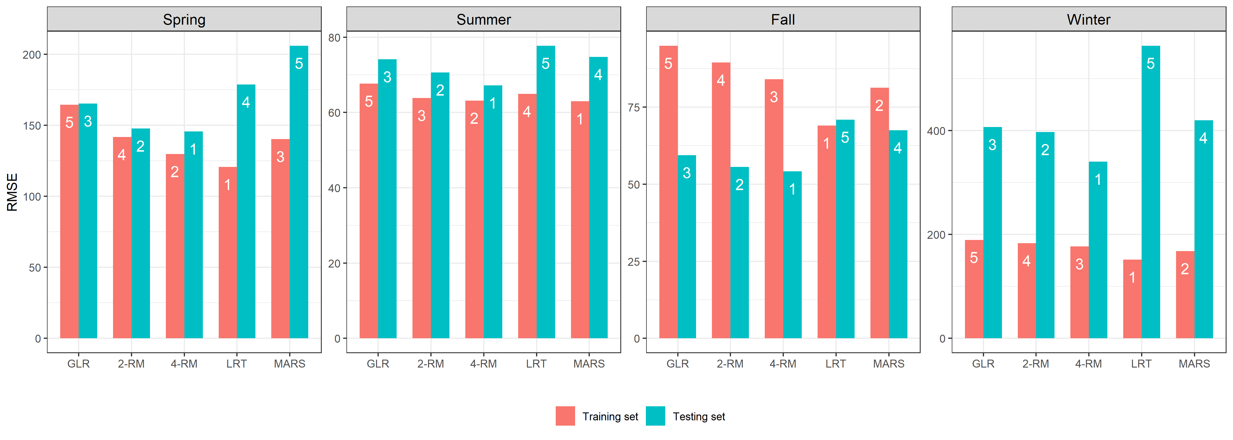
Figure 2 summarizes the in-sample and out-of-sample MSEs of these models in each season. Within the training sets, LRT or MARS achieved the lowest MSE among the five models with the average rank being 1.75 and 2, respectively. Here, rank 1 indicates the best performance. The average rank of the 4-REG in the training groups was 2.5, while those of the 2-REG and GLR ranked the lowest in all seasons. However, LRT and MARS had the highest prediction MSEs on the testing sets, even worse than the benchmark GLR for all seasons, indicating they were severely over-fitted. The segmented linear models, 4-REG and 2-REG, were the best two in terms of out-of-sample performances, with the 4-REG achieving the lowest predictive errors consistently in all seasons.
The estimated 4-regimes models in the spring, summer and fall seasons all had three regimes, as the fourth estimated regime had zero sample size in the three seasons. A further examination suggested that the two estimated boundaries had no intersections over the sample regions, which corresponded to Model (6.1) and reflected the fact that the proposed LS criterion based on the four-regime model may be able to produce a three-regime model if the latter offers better fit. The winter had four estimated regimes. The estimated regression coefficients and their confidence intervals are given in Figure S4 of the SM ([33]).
| Season | TEMP | DEWP | IWS | NE | NW | SE | SW | |||
| Spring | 1 | 1.3 | -2.5 | -0.0 | -0.4 | 0.9 | 0.3 | 0.1 | 0.0 | 0.78 |
| 2 | 0.4 | -0.5 | -0.1 | -0.1 | 0.6 | 0.6 | 0.1 | 0.3 | ||
| Summer | 1 | 1.0 | 5.5 | -12.9 | -0.0 | -12.7 | -15.0 | -8.9 | -9.0 | 0.75 |
| 2 | 0.4 | 0.2 | -0.2 | 0.0 | -0.7 | -0.7 | -0.7 | -0.7 | ||
| Fall | 1 | 0.7 | -1.0 | 0.3 | -0.1 | 0.5 | -0.0 | 0.3 | 0.0 | 0.65 |
| 2 | -0.5 | 1.6 | -1.0 | 0.0 | 0.1 | -1.6 | -1.3 | -0.1 | ||
| Winter | 1 | 0.2 | -0.5 | 0.6 | -0.2 | 0.2 | 0.4 | 0.4 | -0.4 | 0.45 |
| 2 | 0.0 | -0.6 | 0.2 | -0.4 | 1.2 | 1.4 | 0.3 | 1.0 |
Table 4 reports the estimated coefficients of the two splitting boundaries for each season as well as the cosine of the dihedral angle (denoted as ) between the two boundary hyperplanes. It can be seen that for the first three seasons were relatively larger than that in winter, which explains why the boundary hyperplanes of these three seasons were non-intersected. Table 4 indicates that the DEWP and the wind-related variables were the most influential in determining the slopes of the estimated boundaries due to their absolute coefficient values as the was normalized. This reveals an attraction of the proposed regime-splitting mechanism in that the splitting boundaries are determined empirically by multivariate covariates, which contrasts to the threshold regression where the boundary variable has to be user-specified.
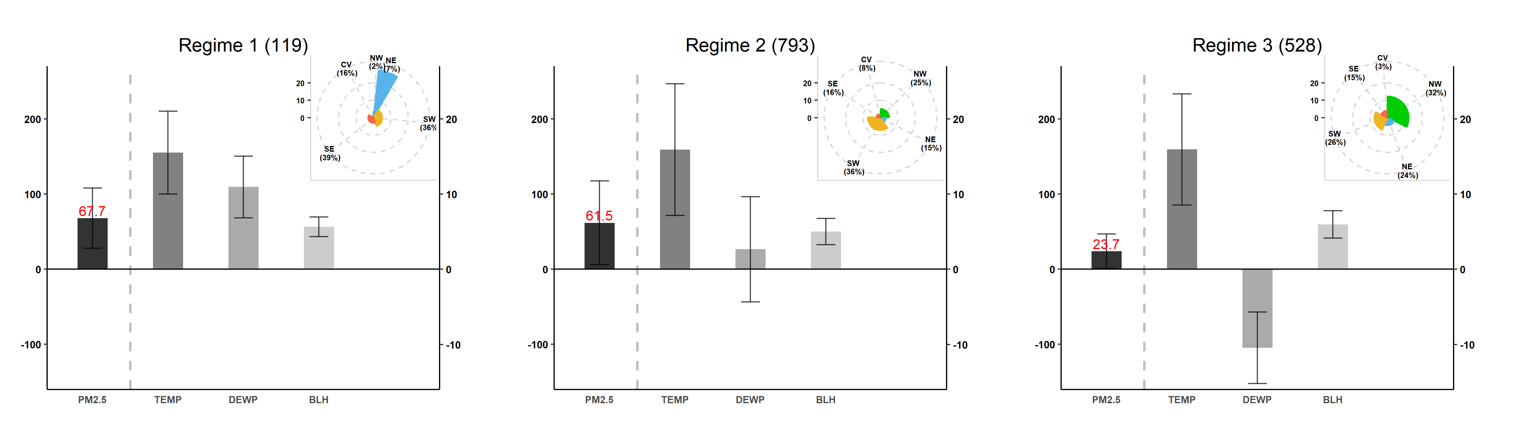
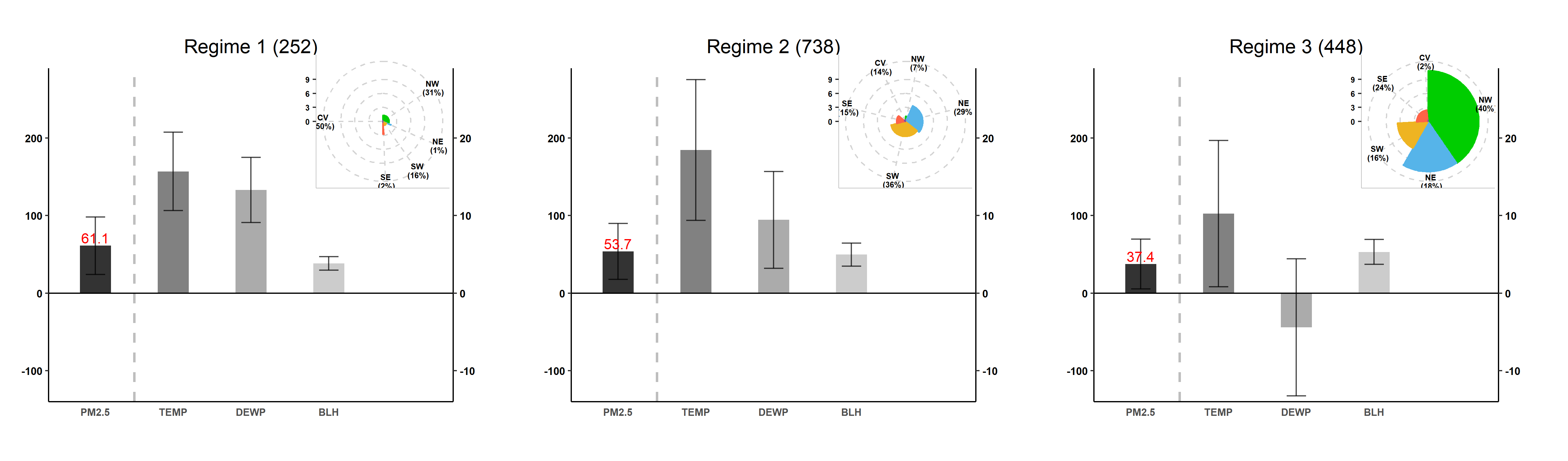
Figure 3(b) displays summary statistics of PM2.5 and the meteorological variables under the three regimes in the spring and fall seasons, as well as the rose plots for the wind directions and the average integrated wind speed (IWS). It shows that the segmented regression picked up three meteorological regimes on PM2.5 where Regime 1 corresponded to the pollution state with high DEWP and high proportion of Calm and Variable wind (CV) which are known to encourage the secondary generation of PM2.5 and unfavorable static atmospheric diffusion, Regime 2 was a transitional state between the clean and high pollution states with reduced DEWP and CV, and Regime 3 was a cleaning state dominated by the northerly wind which brought cleaner and cooler air from the north. Results of the other two seasons and analysis are provided in Figure S5 of the SM.
9 Discussion
This paper develops a statistical inference approach for four-regimes segmented linear models, which broadens the scope of the two-regime models of [22] and [35], and can attains valid inference for degenerated models with less than four regimes. The proposed segmented model is shown to produce better in-sample and out-sample results for the air quality data in Beijing and produced regime-splitting results which had clear atmospheric physics interpretation.
There are two possible extensions which may be considered in future research. One is to allow endogeneity which may be encountered in economic and social behavior applications. If is endogenous and is exogenous, and can be consistently estimated with instrument variables and the two-stage least squares estimation (2SLS) by first regressing on , and then using the fitted to substitute in the four-regime model. The LS estimation via the MIQP and the inference methods for the four-regime model presented in this paper is still applicable. However, the 2SLS is no longer working if is endogenous as discussed in [36], who proposed a conditioning and re-centering approach which might be extended to the four-regime model. Specifically, let , for , and , then Model (2.1) can be written as , which is a partially linear segmented model, where is identifiable without instrument variables. However, the integrated difference kernel estimator used in [36] was designed for univariate threshold, and it is interesting to see how it can be extended to multivariate . Alternatively, one may consider estimating via the mixed integer programming with the nonlinear part approximated via sieve functions. How to solve these issues in the context of the four-regime model requires further investigation.
Another extension is for segmented models with splitting hyperplanes. In general, the splitting hyperplanes in can lead to as many as segments, as shown in Section G of the SM ([33]). It is clear that the investigations in this study for the two boundary case provide vital understanding to the general cases. For example, if we consider an extension to the case of having three hyperplanes in , we can fit a segmented model with regimes by the least squares estimation, whose criterion function would have the same form as (3.1). The backward selection procedure in Section 6 can be employed to specify the optimal number of regimes, and the smoothed regression bootstrap is still able to facilitate the inference for and . Furthermore, the proof for the asymptotic distributions of the least squares estimators can be modified to suit the more general segmented models. The main challenge for the general cases is the complicated model form and demanding computation costs caused by the increase of , requiring efforts in further studies. On the other hand, as grows exponentially with respect to if and polynomially if , there would be little need to consider segmented models with large and as the nonparametric local models (regression trees, etc) may be better suited.
Acknowledgements
The research was partially supported by National Natural Science Foundation of China grants 12292980, 12292983 and 92358303.
Supplement to “Statistical Inference on Four-Regime Segmented Regression Models” \sdescriptionIn the supplementary material, we present technical details, proofs and additional results of the simulations and the case study.
References
- [1] {barticle}[author] \bauthor\bsnmAuerbach, \bfnmAlan J.\binitsA. J. and \bauthor\bsnmGorodnichenko, \bfnmYuriy\binitsY. (\byear2012). \btitleMeasuring the Output Responses to Fiscal Policy. \bjournalAmerican Economic Journal: Economic Policy \bvolume4 \bpages1–27. \bdoi10.1257/pol.4.2.1 \endbibitem
- [2] {barticle}[author] \bauthor\bsnmBai, \bfnmJushan\binitsJ. and \bauthor\bsnmPerron, \bfnmPierre\binitsP. (\byear1998). \btitleEstimating and testing linear models with multiple structural changes. \bjournalEconometrica \bvolume66 \bpages47–78. \bdoi10.2307/2998540 \bmrnumber1616121 \endbibitem
- [3] {barticle}[author] \bauthor\bsnmBertsimas, \bfnmDimitris\binitsD., \bauthor\bsnmKing, \bfnmAngela\binitsA. and \bauthor\bsnmMazumder, \bfnmRahul\binitsR. (\byear2016). \btitleBest subset selection via a modern optimization lens. \bjournalAnn. Statist. \bvolume44 \bpages813–852. \bdoi10.1214/15-AOS1388 \bmrnumber3476618 \endbibitem
- [4] {bbook}[author] \bauthor\bsnmBertsimas, \bfnmDimitris\binitsD. and \bauthor\bsnmWeismantel, \bfnmRobert\binitsR. (\byear2005). \btitleOptimization over Integers \bvolume13. \bpublisherDynamic Ideas Belmont. \endbibitem
- [5] {barticle}[author] \bauthor\bsnmCard, \bfnmDavid\binitsD., \bauthor\bsnmMas, \bfnmAlexandre\binitsA. and \bauthor\bsnmRothstein, \bfnmJesse\binitsJ. (\byear2008). \btitleTipping and the Dynamics of Segregation. \bjournalThe Quarterly Journal of Economics \bvolume123 \bpages177–218. \bdoi10.1162/qjec.2008.123.1.177 \endbibitem
- [6] {barticle}[author] \bauthor\bsnmChan, \bfnmK. S.\binitsK. S. (\byear1993). \btitleConsistency and limiting distribution of the least squares estimator of a threshold autoregressive model. \bjournalAnn. Statist. \bvolume21 \bpages520–533. \bdoi10.1214/aos/1176349040 \bmrnumber1212191 \endbibitem
- [7] {barticle}[author] \bauthor\bsnmChernozhukov, \bfnmVictor\binitsV. and \bauthor\bsnmFernández-Val, \bfnmIván\binitsI. (\byear2011). \btitleInference for extremal conditional quantile models, with an application to market and birthweight risks. \bjournalThe Review of Economic Studies \bvolume78 \bpages559–589. \bdoi10.1093/restud/rdq020 \endbibitem
- [8] {barticle}[author] \bauthor\bsnmChernozhukov, \bfnmVictor\binitsV. and \bauthor\bsnmHong, \bfnmHan\binitsH. (\byear2004). \btitleLikelihood estimation and inference in a class of nonregular econometric models. \bjournalEconometrica \bvolume72 \bpages1445–1480. \bdoi10.1111/j.1468-0262.2004.00540.x \bmrnumber2077489 \endbibitem
- [9] {barticle}[author] \bauthor\bsnmDavies, \bfnmRobert B.\binitsR. B. (\byear1987). \btitleHypothesis testing when a nuisance parameter is present only under the alternative. \bjournalBiometrika \bvolume74 \bpages33–43. \bdoi10.1093/biomet/74.1.33 \bmrnumber885917 \endbibitem
- [10] {barticle}[author] \bauthor\bsnmFan, \bfnmJianqing\binitsJ. and \bauthor\bsnmYao, \bfnmQiwei\binitsQ. (\byear1998). \btitleEfficient estimation of conditional variance functions in stochastic regression. \bjournalBiometrika \bvolume85 \bpages645–660. \bdoi10.1093/biomet/85.3.645 \bmrnumber1665822 \endbibitem
- [11] {barticle}[author] \bauthor\bsnmFriedman, \bfnmJerome H.\binitsJ. H. (\byear1991). \btitleMultivariate adaptive regression splines. \bjournalAnn. Statist. \bvolume19 \bpages1–141. \bnoteWith discussion and a rejoinder by the author. \bdoi10.1214/aos/1176347963 \bmrnumber1091842 \endbibitem
- [12] {barticle}[author] \bauthor\bsnmGonzalo, \bfnmJesús\binitsJ. and \bauthor\bsnmPitarakis, \bfnmJean-Yves\binitsJ.-Y. (\byear2002). \btitleEstimation and model selection based inference in single and multiple threshold models. \bjournalJ. Econometrics \bvolume110 \bpages319–352. \bnoteLong memory and nonlinear time series (Cardiff, 2000). \bdoi10.1016/S0304-4076(02)00098-2 \bmrnumber1928308 \endbibitem
- [13] {barticle}[author] \bauthor\bsnmGonzalo, \bfnmJesús\binitsJ. and \bauthor\bsnmWolf, \bfnmMichael\binitsM. (\byear2005). \btitleSubsampling inference in threshold autoregressive models. \bjournalJ. Econometrics \bvolume127 \bpages201–224. \bdoi10.1016/j.jeconom.2004.08.004 \bmrnumber2156333 \endbibitem
- [14] {bbook}[author] \bauthor\bsnmGyörfi, \bfnmLázló\binitsL., \bauthor\bsnmHärdle, \bfnmWolfgang\binitsW., \bauthor\bsnmSarda, \bfnmPascal\binitsP. and \bauthor\bsnmVieu, \bfnmPhilippe\binitsP. (\byear1989). \btitleNonparametric curve estimation from time series. \bseriesLecture Notes in Statistics \bvolume60. \bpublisherSpringer-Verlag, Berlin. \endbibitem
- [15] {barticle}[author] \bauthor\bsnmHansen, \bfnmBruce E.\binitsB. E. (\byear1996). \btitleInference when a nuisance parameter is not identified under the null hypothesis. \bjournalEconometrica \bvolume64 \bpages413–430. \bdoi10.2307/2171789 \bmrnumber1375740 \endbibitem
- [16] {barticle}[author] \bauthor\bsnmHansen, \bfnmBruce E.\binitsB. E. (\byear2000). \btitleSample splitting and threshold estimation. \bjournalEconometrica \bvolume68 \bpages575–603. \bdoi10.1111/1468-0262.00124 \bmrnumber1769379 \endbibitem
- [17] {barticle}[author] \bauthor\bsnmHärdle, \bfnmWolfgang\binitsW., \bauthor\bsnmHorowitz, \bfnmJoel\binitsJ. and \bauthor\bsnmKreiss, \bfnmJens-Peter\binitsJ.-P. (\byear2003). \btitleBootstrap methods for time series. \bjournalInternational Statistical Review \bvolume71 \bpages435–459. \endbibitem
- [18] {barticle}[author] \bauthor\bsnmHsing, \bfnmTailen\binitsT. (\byear1995). \btitleOn the asymptotic independence of the sum and rare values of weakly dependent stationary random variables. \bjournalStochastic Process. Appl. \bvolume60 \bpages49–63. \bdoi10.1016/0304-4149(95)00054-2 \bmrnumber1362318 \endbibitem
- [19] {barticle}[author] \bauthor\bsnmJiang, \bfnmZhenyu\binitsZ., \bauthor\bsnmDu, \bfnmChengan\binitsC., \bauthor\bsnmJablensky, \bfnmAssen\binitsA., \bauthor\bsnmLiang, \bfnmHua\binitsH., \bauthor\bsnmLu, \bfnmZudi\binitsZ., \bauthor\bsnmMa, \bfnmYang\binitsY. and \bauthor\bsnmTeo, \bfnmKok Lay\binitsK. L. (\byear2014). \btitleAnalysis of schizophrenia data using a nonlinear threshold index logistic model. \bjournalPloS ONE \bvolume9 \bpagese109454. \bdoi10.1371/journal.pone.0109454 \endbibitem
- [20] {barticle}[author] \bauthor\bsnmKhalili, \bfnmAbbas\binitsA. and \bauthor\bsnmChen, \bfnmJiahua\binitsJ. (\byear2007). \btitleVariable selection in finite mixture of regression models. \bjournalJ. Amer. Statist. Assoc. \bvolume102 \bpages1025–1038. \bdoi10.1198/016214507000000590 \bmrnumber2411662 \endbibitem
- [21] {bmisc}[author] \bauthor\bsnmKnight, \bfnmK\binitsK. (\byear1999). \btitleEpi-convergence and stochastic equisemicontinuity. \bnotePreprint. \endbibitem
- [22] {barticle}[author] \bauthor\bsnmLee, \bfnmSokbae\binitsS., \bauthor\bsnmLiao, \bfnmYuan\binitsY., \bauthor\bsnmSeo, \bfnmMyung Hwan\binitsM. H. and \bauthor\bsnmShin, \bfnmYoungki\binitsY. (\byear2021). \btitleFactor-driven two-regime regression. \bjournalAnn. Statist. \bvolume49 \bpages1656–1678. \bdoi10.1214/20-aos2017 \bmrnumber4298876 \endbibitem
- [23] {barticle}[author] \bauthor\bsnmLi, \bfnmDong\binitsD. and \bauthor\bsnmLing, \bfnmShiqing\binitsS. (\byear2012). \btitleOn the least squares estimation of multiple-regime threshold autoregressive models. \bjournalJ. Econometrics \bvolume167 \bpages240–253. \bdoi10.1016/j.jeconom.2011.11.006 \bmrnumber2885449 \endbibitem
- [24] {barticle}[author] \bauthor\bsnmLiu, \bfnmRegina Y.\binitsR. Y. (\byear1988). \btitleBootstrap procedures under some non-i.i.d. models. \bjournalAnn. Statist. \bvolume16 \bpages1696–1708. \bdoi10.1214/aos/1176351062 \bmrnumber964947 \endbibitem
- [25] {barticle}[author] \bauthor\bsnmMeyer, \bfnmR. M.\binitsR. M. (\byear1973). \btitleA Poisson-type limit theorem for mixing sequences of dependent “rare” events. \bjournalAnn. Probability \bvolume1 \bpages480–483. \bdoi10.1214/aop/1176996941 \bmrnumber350816 \endbibitem
- [26] {barticle}[author] \bauthor\bsnmPolitis, \bfnmDimitris N.\binitsD. N. and \bauthor\bsnmRomano, \bfnmJoseph P.\binitsJ. P. (\byear1994). \btitleLarge sample confidence regions based on subsamples under minimal assumptions. \bjournalAnn. Statist. \bvolume22 \bpages2031–2050. \bdoi10.1214/aos/1176325770 \bmrnumber1329181 \endbibitem
- [27] {barticle}[author] \bauthor\bsnmPotter, \bfnmSimon M.\binitsS. M. (\byear1995). \btitleA nonlinear approach to US GNP. \bjournalJournal of Applied Econometrics \bvolume10 \bpages109-125. \bdoihttps://doi.org/10.1002/jae.3950100203 \endbibitem
- [28] {bbook}[author] \bauthor\bsnmResnick, \bfnmSidney I.\binitsS. I. (\byear2008). \btitleExtreme values, regular variation and point processes. \bseriesSpringer Series in Operations Research and Financial Engineering. \bpublisherSpringer, New York. \bmrnumber2364939 \endbibitem
- [29] {barticle}[author] \bauthor\bsnmSchwartz, \bfnmPamela F\binitsP. F., \bauthor\bsnmGennings, \bfnmChris\binitsC. and \bauthor\bsnmChinchilli, \bfnmVernon M\binitsV. M. (\byear1995). \btitleThreshold models for combination data from reproductive and developmental experiments. \bjournalJournal of the American Statistical Association \bvolume90 \bpages862–870. \bdoi10.1080/01621459.1995.10476585 \endbibitem
- [30] {barticle}[author] \bauthor\bsnmSchwarz, \bfnmGideon\binitsG. (\byear1978). \btitleEstimating the dimension of a model. \bjournalAnn. Statist. \bvolume6 \bpages461–464. \bmrnumber468014 \endbibitem
- [31] {barticle}[author] \bauthor\bsnmSeijo, \bfnmEmilio\binitsE. and \bauthor\bsnmSen, \bfnmBodhisattva\binitsB. (\byear2011). \btitleChange-point in stochastic design regression and the bootstrap. \bjournalAnn. Statist. \bvolume39 \bpages1580–1607. \bdoi10.1214/11-AOS874 \bmrnumber2850213 \endbibitem
- [32] {bbook}[author] \bauthor\bsnmTong, \bfnmHowell\binitsH. (\byear1983). \btitleThreshold Models in Non-linear Time Series Analysis. Lecture Notes in Statistics, No. 21. \bpublisherSpringer-Verlag. \endbibitem
- [33] {barticle}[author] \bauthor\bsnmYan, \bfnmHan\binitsH. and \bauthor\bsnmChen, \bfnmSong Xi\binitsS. X. (\byear2024). \btitleSupplement to “Statistical Inference for Four-Regime Segmented Regression Models”. \endbibitem
- [34] {barticle}[author] \bauthor\bsnmYu, \bfnmPing\binitsP. (\byear2014). \btitleThe bootstrap in threshold regression. \bjournalEconometric Theory \bvolume30 \bpages676–714. \bdoi10.1017/S0266466614000012 \bmrnumber3205610 \endbibitem
- [35] {barticle}[author] \bauthor\bsnmYu, \bfnmPing\binitsP. and \bauthor\bsnmFan, \bfnmXiaodong\binitsX. (\byear2021). \btitleThreshold regression with a threshold boundary. \bjournalJournal of Business & Economic Statistics \bvolume39 \bpages953–971. \bdoi10.1080/07350015.2020.1740712 \endbibitem
- [36] {barticle}[author] \bauthor\bsnmYu, \bfnmPing\binitsP. and \bauthor\bsnmPhillips, \bfnmPeter C. B.\binitsP. C. B. (\byear2018). \btitleThreshold regression with endogeneity. \bjournalJ. Econometrics \bvolume203 \bpages50–68. \bdoi10.1016/j.jeconom.2017.09.007 \bmrnumber3758327 \endbibitem
- [37] {barticle}[author] \bauthor\bsnmZeileis, \bfnmAchim\binitsA., \bauthor\bsnmHothorn, \bfnmTorsten\binitsT. and \bauthor\bsnmHornik, \bfnmKurt\binitsK. (\byear2008). \btitleModel-based recursive partitioning. \bjournalJ. Comput. Graph. Statist. \bvolume17 \bpages492–514. \bdoi10.1198/106186008X319331 \bmrnumber2439970 \endbibitem