Random non-Hermitian Hamiltonian framework for symmetry breaking dynamics

Abstract

We propose random non-Hermitian Hamiltonians to model the generic stochastic nonlinear dynamics of a quantum state in Hilbert space. Our approach features an underlying linearity in the dynamical equations, ensuring the applicability of techniques used for solving linear systems. Additionally, it offers the advantage of easily incorporating statistical symmetry, a generalization of explicit symmetry to stochastic processes. To demonstrate the utility of our approach, we apply it to describe real-time dynamics, starting from an initial symmetry-preserving state and evolving into a randomly distributed, symmetry-breaking final state. Our model serves as a quantum framework for the transition process, from disordered states to ordered ones, where symmetry is spontaneously broken.

Introduction.—The Schrödinger equation is both deterministic and linear, forming the foundation of quantum mechanics. Since the 1990s, however, efforts have been made to generalize the Schrödinger equation into stochastic nonlinear differential equations GRW ; Diosi89 ; Bassi05 ; CSL ; CSL2 ; Penrose96 ; Pearle99 ; Adler07 ; Adler08 ; Bassi13 ; Pontin19 ; Vinante17 ; Donadi21 ; Bahrami18 ; Tilloy19 ; Gasbarri21 ; Vinante16 ; Vinante20 ; Carlesso22 ; Zheng20 ; Komori20 ; Gisin92 ; Percival98 ; Plenio98 ; Daley14 ; Castin95 ; Power96 ; Ates12 ; Hu13 ; Raghunandan18 ; Pokharel18 ; Weimer21 ; Weimer22 . There are two primary motivations for this generalization. The first is to provide an explanation for the objective wave function collapse during quantum measurement, which leads to spontaneous collapse models GRW ; Diosi89 ; Bassi05 ; CSL ; CSL2 ; Penrose96 ; Pearle99 ; Adler07 ; Adler08 ; Bassi13 . These models differ from conventional quantum mechanics and have recently seen renewed interest, with numerous experimental platforms being proposed to test them Pontin19 ; Vinante17 ; Donadi21 ; Bahrami18 ; Tilloy19 ; Gasbarri21 ; Vinante16 ; Vinante20 ; Carlesso22 ; Zheng20 ; Komori20 . The second motivation arises from the study of open quantum systems, where master equations for the density matrix can be unraveled into stochastic nonlinear equations Gisin92 ; Percival98 ; Plenio98 ; Daley14 . These unravelled equations have found applications in quantum optics Castin95 ; Power96 ; Ates12 ; Hu13 ; Raghunandan18 ; Pokharel18 ; Weimer21 ; Weimer22 . Despite these studies, a general framework for quantum stochastic nonlinear dynamics remains elusive, primarily due to the challenges in solving nonlinear equations and incorporating symmetries—such as Lorentz symmetry—into the formalism Myrvold17 ; Tumulka20 ; Jones20 ; Jones21 . This highlights the need for new approaches.

In this paper, we demonstrate that stochastic nonlinear dynamics can be equivalently generated by linear evolution operators governed by random non-Hermitian (RNH) Hamiltonians. While there has been extensive research on non-Hermitian Hamiltonians, particularly with or without PT-symmetry Bender07 , in the dynamics of open quantum systems, including quantum scattering Rotter09 and non-Hermitian topological insulators Hatano96 ; Xiong18 ; Alvarez18 ; Wang18 ; Gong18 ; Kunst18 ; Kawabata19 ; Budich19 ; Budich20 ; WangZ22 ; Xue21 ; Wang24 , as well as in classical optical, mechanical, and electrical systems Ganainy18 ; Kunst21 , these models differ from ours in that they do not incorporate temporal noise or stochastic processes, which are critical to our approach.

Our method offers several advantages. It retains a hidden linearity in the equations, which not only simplifies solving them but also naturally reveals the symmetry of the system—a feature that was challenging to access in previous approaches. In fact, in the presence of temporal noise, the conventional concept of quantum symmetry (explicit symmetry) must be replaced by statistical symmetry Wang22 . Statistical symmetry refers to the invariance of the probability distribution of an ensemble of quantum-state trajectories under symmetry transformations, even though individual random trajectories may not remain invariant.

We demonstrate the application of RNH-Hamiltonians with statistical symmetry by exploring real-time dynamics leading to spontaneous symmetry breaking (SSB). While SSB is a well-established concept in equilibrium statistical mechanics, its corresponding dynamical process remains poorly understood. Consider the $\text{Z}_{2}$-symmetric transverse-field Ising model at zero temperature. Suppose the system begins in a symmetry-preserving initial state, with all spins aligned in the transverse direction, corresponding to the ground state in the strong-field limit. As the field is withdrawn, the spins relax to the zero-field ground states, which are ferromagnetic states that spontaneously break $\text{Z}_{2}$ symmetry. During this evolution, the system must ”choose” between two degenerate states (spin-up or spin-down), each with a 50% probability, determined by uncontrollable environmental perturbations. This makes the process inherently stochastic, while still respecting $\text{Z}_{2}$ symmetry. Furthermore, the system does not evolve into a superposition of spin-up and spin-down states, even though such a superposition would also possess the same ground-state energy due to $\text{Z}_{2}$ symmetry. To understand why the superposition is ruled out, we must account for the role of the environment, which selects the pointer states (spin-up or spin-down) from an infinite set of degenerate superposition states. To the best of our knowledge, no existing models explain this process.

In this paper, we demonstrate that this process can indeed be described using RNH-Hamiltonians. We not only construct an exactly solvable benchmark model but also investigate more general RNH-Hamiltonians that are not strictly solvable. To tackle these, we develop a robust stochastic semiclassical method for approximating solutions. Our work lays the foundation for the RNH-Hamiltonian theory of stochastic nonlinear quantum dynamics.

Exactly solvable model.—Our RNH models can be conveniently expressed using an infinitesimal Hamiltonian integral Wang22 , defined as

$$d\hat{H}_{t}=\hat{H}_{0}\ dt+i\hat{V}\ dW_{t},$$ (1)

where the first term represents the Hermitian Hamiltonian acting over an infinitesimal time interval, while the second term accounts for the random non-Hermitian contribution. Here, $dW_{t}$ denotes the differential of a Wiener process, and $\hat{V}$ is a Hermitian operator. The prenormalized quantum state evolves as $\ket{\phi_{t+dt}}=e^{-id\hat{H}_{t}}\ket{\phi_{t}}$, with the infinitesimal evolution operator $\hat{U}_{dt}=e^{-id\hat{H}_{t}}$. When $\hat{V}=0$, $\hat{U}_{dt}$ describes the conventional deterministic unitary evolution. However, for general $\hat{V}\neq 0$, $\hat{U}_{dt}$ leads to a nonunitary and stochastic evolution.

In our theory, the physical state is represented by the normalized state vector, $\ket{\psi_{t}}=\ket{\phi_{t}}/\sqrt{\braket{\phi_{t}}{\phi_{t}}}$, which satisfies the following stochastic nonlinear equation OurSI :

$$\begin{split}&\ket{d\psi_{t}}=-i\hat{H}_{0}dt\ket{\psi_{t}}+dW_{t}\left[\hat{V}-\langle\hat{V}\rangle\right]\ket{\psi_{t}}\\ &+dt\left\{\frac{1}{2}\left[\hat{V}-\langle\hat{V}\rangle\right]^{2}-\left[\langle\hat{V}^{2}\rangle-\langle\hat{V}\rangle^{2}\right]\right\}\ket{\psi_{t}},\end{split}$$ (2)

where $\langle\hat{V}\rangle=\bra{\psi_{t}}\hat{V}\ket{\psi_{t}}$. Note the similarities and differences between Eq. (LABEL:eq:m:non) and the CSL model CSL ; CSL2 . A key advantage of the RNH approach is that it avoids the need to directly solve Eq. (LABEL:eq:m:non), Instead, we can solve the much simpler linear equation for $\ket{\phi_{t}}$, and then normalize it to obtain $\ket{\psi_{t}}$ at the final time.

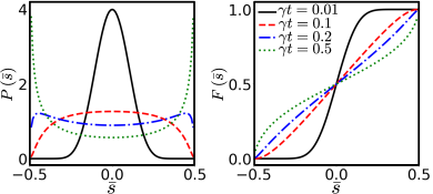
Figure 1: Probability density and cumulant distribution functions at different times.

To be specific, we consider a system of $N$ spin-$1/2$ particles exhibiting $\text{Z}_{2}$ symmetry, with the symmetry operator defined as $\hat{X}=\otimes\prod_{j}\hat{\sigma}_{j}^{x}$, which flips all spins in the $z$-direction simultaneously. Let $\hat{V}=\sqrt{\gamma}\hat{\sigma}_{z}$, where $\hat{\sigma}_{z}=\sum_{j}\hat{\sigma}_{j}^{z}$ is the total spin in the $z$-direction, and $\gamma$ represents the noise strength with the dimension of energy (or the inverse of time). First, we set $\hat{H}_{0}=0$, rendering the model exactly solvable. Since $\hat{X}\hat{\sigma}_{z}\hat{X}=-\hat{\sigma}_{z}$, it is straightforward to see that $\hat{X}d\hat{H}_{t}\hat{X}=-d\hat{H}_{t}\neq d\hat{H}_{t}$, meaning that the model (1) does not exhibit explicit $\text{Z}_{2}$ symmetry. However, the Wiener process is symmetrically distributed around zero, or equivalently, in probabilistic terms, $dW_{t}\stackrel{{\scriptstyle d}}{{=}}-dW_{t}$, where $\stackrel{{\scriptstyle d}}{{=}}$ denotes equality in distribution. This leads to $\hat{X}d\hat{H}_{t}\hat{X}\stackrel{{\scriptstyle d}}{{=}}d\hat{H}_{t}$ and, consequently, $\hat{X}\hat{U}_{t}\hat{X}\stackrel{{\scriptstyle d}}{{=}}\hat{U}_{t}$, where $\hat{U}_{t}$ is the evolution operator over a finite time interval. This defines what we term statistical symmetry. Since the symmetry operator $\hat{X}$ is unitary (or antiunitary), it preserves the length of vectors in Hilbert space, ensuring that the normalized dynamical equation (LABEL:eq:m:non) remains invariant under $\hat{X}$. Statistical $\text{Z}_{2}$ symmetry implies that the ensemble of quantum-state trajectories retains the same distribution under the transformation $\hat{X}$. To see this, consider a symmetry-preserving initial state $\hat{X}\ket{\psi_{0}}=\ket{\psi_{0}}$, where all spins are aligned along the positive $x$-direction. Under this condition, it follows that $\hat{X}\ket{\psi_{t}}\stackrel{{\scriptstyle d}}{{=}}\ket{\psi_{t}}$ for arbitrary $t$.

The model (1) with $\hat{V}=\sqrt{\gamma}\hat{\sigma}_{z}$ describes a dynamical process leading to SSB. To demonstrate this, we use the Dicke basis $\ket{s}$, where $s=\sum_{j}\sigma^{z}_{j}/2N$ represents the average magnetization, and consider the wave packet $\phi(t,s)=\braket{s}{\phi_{t}}=e^{2Ns\sqrt{\gamma}W_{t}}\psi_{0}(s)$. The symmetry transformation $\hat{X}\ket{s}=\ket{-s}$ applies here. In the study of SSB, the thermodynamic limit $N\to\infty$ is critical, and we then impose the large-$N$ condition. For sufficiently large $N$, using Stirling’s formula, we find that $\phi(t,s)$ exhibits a sharp peak, with a width of $\sim 1/\sqrt{N}$, collapsing to a delta function in the $N\to\infty$ limit OurSI . In other words, the wave packet localizes at some point in $s$-space.

Due to the stochastic nature of the dynamics, the peak location of the wave packet becomes a time-dependent random variable, $\bar{s}$, defined by $\partial_{s}\left|\psi(t,s)\right|^{2}=0$ at ${s=\bar{s}}$. A straightforward calculation gives $\bar{s}=\frac{1}{2}\tanh\left(\tilde{W}_{t}\right)$, where $\tilde{W}_{t}\equiv 2\sqrt{\gamma}W_{t}$, and $W_{t}$ is the Wiener process at time $t$, with the initial time set to $t_{0}=0$. The probability distribution of $\bar{s}$ can be more conveniently expressed using the rescaled magnetization $\bar{m}=\ln\frac{1+2\bar{s}}{1-2\bar{s}}$, a one-to-one mapping from $\bar{s}\in\left(-1/2,1/2\right)$ to $\bar{m}\in(-\infty,\infty)$. The variable $\bar{m}$ follows a Gaussian distribution with mean zero and variance $16\gamma t$ OurSI . The cumulant distribution of $\bar{s}$ is $F(\bar{s})=\Phi\left(\bar{m}\left(\bar{s}\right)/\sqrt{16\gamma t}\right)$, where $\Phi$ is the cumulative distribution function of the normal Gaussian distribution. Figure 1 illustrates $P(\bar{s})$ and $F(\bar{s})$ at different times.

At time $t=0$, the probability density is $P(\bar{s})=\delta(\bar{s})$, corresponding to zero magnetization, reflecting the explicit $\text{Z}_{2}$ symmetry of the initial state. As time progresses, $P(\bar{s})$ flattens (see Fig. 1 the left panel), but remains symmetric about zero due to statistical symmetry, which enforces $P(\bar{s})=P(-\bar{s})$. Over time, the probability shifts from $\bar{s}=0$ to $\bar{s}=\pm 1/2$, eventually forming two peaks at $\bar{s}=\pm 1/2$. In the limit as $t\to\infty$, the probability distribution becomes $P(\bar{s})=\frac{1}{2}(\delta(\bar{s}+\frac{1}{2})+\delta(\bar{s}-\frac{1}{2})$. The all-spin-up and all-spin-down states both occur with probability $1/2$, but superpositions of these states do not persist, as desired.

Notably, the states $\ket{\bar{s}=\pm 1/2}$ are ferromagnetic and spontaneously break $\text{Z}_{2}$ symmetry, yet the overall distribution respects statistical symmetry, as the probabilities of $\bar{s}=1/2$ and $\bar{s}=-1/2$ are equal. The timescale for symmetry breaking is characterized by $1/\gamma$. For $t\ll 1/\gamma$, the probability remains concentrated around $\bar{s}=0$ (the symmetry-preserving state), while for $t\gg 1/\gamma$, it converges at $\bar{s}=\pm 1/2$ (the SSB states).

Stochastic semiclassical approach.—Next, we examine the impact of a Hermitian term, $\hat{H}_{0}$, on the dynamics. Specifically, we consider the prototypical transverse-field Ising Hamiltonian: $\hat{H}_{0}=-\frac{J}{N}\hat{\sigma}_{z}^{2}+h\hat{\sigma}_{x}$, where $J>0$ represents the ferromagnetic coupling and $h>0$ represents the transverse field. It is easy to see that $\hat{H}_{0}=\hat{X}\hat{H}_{0}\hat{X}$, which displays $\text{Z}_{2}$ symmetry. Therefore, adding it to $d\hat{H}_{t}$ preserves the statistical $\text{Z}_{2}$-symmetry. The ground state of $\hat{H}_{0}$ undergoes a quantum phase transition at $h=2J$, spontaneously breaking the $\text{Z}_{2}$ symmetry for $h<2J$.

When $h\neq 0$, Eq (1) is no longer strictly solvable. To obtain an approximate solution for large $N$, we develop the stochastic semiclassical approach. The key idea is that, for sufficiently large $N$, the wave function at any time $t$ exhibits a sharp peak in $s$-space. Consequently, we can focus on the location of the peak, denoted by $\bar{s}$, while neglecting the detailed form of $\phi(t,s)$. To determine $\bar{s}(t)$, we first express $\phi(t,s)$ as $\phi(t,s)=\exp\left\{-N\left(g(t,s)-i\theta(t,s)\right)\right\}$, and derive the dynamical equations for $g(t,s)$ and $\theta(t,s)$. The peak location $\bar{s}(t)$ corresponds to the minimum of $g(t,s)$. By expanding $g(t,s)$ and $\theta(t,s)$ around $\bar{s}$ using a Taylor series and substituting into the dynamical equations, we find:

$$\begin{split}&d\bar{s}=d\left(\frac{1}{2}\tanh\left(\tilde{W}_{t}\right)\right)-\tilde{f}(\bar{s})\sin\left(\bar{p}\right)\ dt,\\ &d\bar{p}=4h^{2}\ \bar{s}\tilde{f}(\bar{s})^{-1}\cos(\bar{p})\ dt+4Jt\ d\left(\tanh\left(\tilde{W}_{t}\right)\right)+8J\bar{s}\ dt,\end{split}$$ (3)

where $\tilde{f}(s)=2h\sqrt{\frac{1}{4}-s^{2}}$, and $\bar{p}=\partial_{s}\theta\left|{}_{s=\bar{s}}\right.$ represents the classical momentum (see Appendix for the detail of derivation). As $\gamma=0$, Eq. (3) reduces to the classical equations of motion governed by the Hamiltonian $H_{0}(\bar{s},\bar{p})=\tilde{f}(s)\cos\bar{p}-4J\bar{s}^{2}$, which is well known in the semiclassical treatment of fully-connected models Sciolla11 . A systematic perturbative approach can be applied to solve Eq. (3). To first order of $h$, the solution is given by:

$$\begin{split}&\bar{s}(t)\approx\bar{s}_{0}(t)-h\int^{t}_{0}d\tau\sqrt{X_{\tau}}\sin\left[8J\tau\bar{s}_{0}(\tau)\right],\\ &\bar{p}(t)\approx 8Jt\bar{s}_{0}(t)+4h\int^{t}_{0}d\tau\frac{\bar{s}_{0}(\tau)}{\sqrt{X_{\tau}}}\cos\left[8J\tau\bar{s}_{0}(\tau)\right],\end{split}$$ (4)

where $\bar{s}_{0}(t)=\frac{1}{2}\tanh\left(\tilde{W}_{t}\right)$ is the exact solution for $h=0$, and $X_{\tau}=1-4\bar{s}_{0}(\tau)^{2}$. Our numerical simulations verify that solutions (4) provide good approximations OurSI , except when $\gamma t\gg 1$, at which point they predict unphysical results ($\left|\bar{s}\right|>1/2$). The behavior for $\gamma t\gg 1$ will be discussed separately. We emphasize that our approach is applicable to general RNH-Hamiltonians in a broad class of full-connected models.

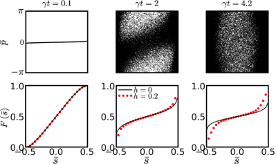
Figure 2: Top panels: Samples of random variables $\left(\bar{s},\bar{p}\right)$ plotted in the $\bar{s}-\bar{p}$ plane at different times—$\gamma t=0.1$, $2$, and $4.2$ from left to right. Parameters are chosen as $h=0.2$ and $J=0.1$. $\left(\bar{s},\bar{p}\right)$ are sampled $10^{5}$ times. Bottom panels: The corresponding cumulant distribution functions (red dots). For comparison, the black solid line represents the cumulant distribution function at $h=0$.

Real-time dynamics when $h\neq 0$.—Next, we set $\gamma=1$ as the unit of energy and examine how $h$ and $J$ affect the probability migration from symmetry-preserved to SSB states, using Eq. (4). The probability migration is indicated by the slope of $F(\bar{s})$ (i.e. $P(\bar{s})$) at $\bar{s}=\pm 1/2$, which increases from zero to infinity, or by the slope at $\bar{s}=0$, which decreases from infinity towards zero. Figure 2 (bottom panels) shows $F(\bar{s})$ for $h=0.2$ (red dots) at different times. We observe no significant deviation from the exact solution (black solid line) until after $t\sim 2$, after which the deviation becomes more pronounced at later times (e.g., $t=4.2$). This deviation indicates that probability migration is hindered. At $t=4.2$, the red dots show a steeper slope at $\bar{s}=0$ and a shallower one at $\bar{s}=\pm 1/2$ compared to the black solid line, suggesting that the development of SSB is being impeded by the transverse field $h$. This aligns with the fact that quantum fluctuations induced by the transverse field disrupt the ferromagnetic order in equilibrium. We explored different parameter values OurSI and found qualitatively similar behavior, with the deviation occuring earlier (later) as $h$ increases (decreases).

Figure 2 (top panels) shows the distribution of $\left(\bar{s},\bar{p}\right)$ in the phase space, revealing a correlation between these variables at early and intermediate times ($t=2$), but this correlation vanishes over time. At $t=0.01$ or $t=0.1$ (early times), the $\gamma$-term dominates, dispersing $\bar{s}$ away from the origin while stretching the set of points in the $\bar{p}$-direction in a counterclockwise manner (as seen from the expression for $\bar{p}$ in Eq. (4)). Meanwhile, $\hat{H}_{0}$ causes a counterclockwise rotation of the $\left(\bar{s},\bar{p}\right)$ points, as predicted by classical Hamiltonian dynamics governed by $H_{0}(\bar{s},\bar{p})$ OurSI . The combined effect of the $\gamma$-term and $\hat{H}_{0}$ leads to an asymmetric distribution at $t=2$. However, at sufficiently long times ($t=4.2$), the asymmetry and $\bar{s}-\bar{p}$ correlation disappear, resulting in an almost uniform probability density along the $\bar{p}$-direction, suggesting that $P(\bar{s},\bar{p})$ becomes independent of $\bar{p}$ in the long-time limit.

Our perturbative results (4) break down when $t\gg 1/h$. To gain a qualitative understanding of the steady-state distribution, we revisit Eq. (3). In the limit $t\to\infty$, $\tanh\left(\tilde{W}_{t}\right)\to\pm 1$ and $d\tanh\left(\tilde{W}_{t}\right)\to 0$, allowing us to neglect the $\gamma$-terms. In this case, Eq. (3) simplifies to the classical dynamical equation governed by $H_{0}(\bar{s},\bar{p})$, and the corresponding Fokker-Planck equation is worked out to be

$$\begin{split}\partial_{t}P(\bar{s},\bar{p},t)=&\ \partial_{\bar{s}}\left[\tilde{f}(\bar{s})\sin\left(\bar{p}\right)P(\bar{s},\bar{p},t)\right]\\ &-\partial_{\bar{p}}\left[\left(2h\frac{\bar{s}}{\sqrt{\frac{1}{4}-\bar{s}^{2}}}\cos(\bar{p})+8J\bar{s}\right)\cdot P(\bar{s},\bar{p},t)\right].\end{split}$$ (5)

By setting $\partial_{t}P=0$, we find the condition for the steady-state distribution. Based on our earlier observation—$\partial_{\bar{p}}P(\bar{s},\bar{p})=0$ in the steady-state limit—we conclude that $\partial_{\bar{s}}P(\bar{s},\bar{p})=0$ as long as $\bar{s}\neq 1/2$. This implies that the steady-state distribution is surprisingly simple: the probability density for $-1/2<\bar{s}<1/2$ must be constant, denoted as $\Delta$, with $0\leq\Delta\leq 1$. The probabilities of $\bar{s}=\pm 1/2$ are both $\left(1-\Delta\right)/2$ due to statistical symmetry. The parameter $\Delta$ is called the residue probability, representing the portion of the probability that has not migrated to the SSB state $\ket{\bar{s}=\pm 1/2}$. The exact solution for $h=0$ corresponds to $\Delta=0$, indicating no residue probability and complete symmetry breaking.

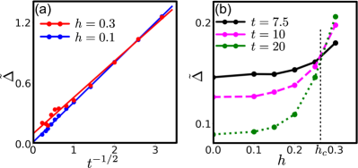
Figure 3: (a) Residue probability $\tilde{\Delta}$ as a function of $t^{-1/2}$ for different values of $h$. The dots represent numerical results, while the solid lines correspond to fitted curves. (b) $\tilde{\Delta}$ as a function of $h$ at different times. The curves intersect at approximately $h_{c}\approx 0.26$. The probability distribution is obtained by sampling $4\times 10^{5}$ times. The parameter $J$ is set to $0.2$.

Incomplete SSB in steady-state distribution.—We numerically investigate the behavior of $\Delta$ for $h\neq 0$. To calculate $\Delta$, we first compute the finite-time residue probability, defined as $\tilde{\Delta}(t)=\text{Pr}(-r<\bar{s}<r)/2r$, where $r$ is chosen to be sufficiently small so that $\tilde{\Delta}(t)$ accurately reflects the probability density at $\bar{s}=0$. In practice, $r=0.05$ is sufficiently small because the probability density in the range $\bar{s}\in[-0.05,0.05]$ is approximately constant as long as $t\geq 0.1$ (see Fig. 1). For $h=0$, the exact solution suggests $\tilde{\Delta}(t)=1/\sqrt{2\pi t}$. Therefore, we expect $\tilde{\Delta}(t)$ to exhibit a similar ${t}^{-1/2}$ decay for nonzero $h$. Figure 3(a) plots $\tilde{\Delta}(t)$ as a function of ${t}^{-1/2}$ (blue and red dots), and the solid lines represent fits to the curve $\tilde{\Delta}(t)=c{t}^{-1/2}+\Delta$. For $h=0.1$ (blue dots), the fit is excellent, and the asymptotic residue probability is found to be close to zero ($\Delta=0.01$ indeed). However, for $h=0.3$ (red dots), we observe oscillations in $\tilde{\Delta}(t)$ in addition to the ${t}^{-1/2}$ decay. More important, the steady-state value improves significantly to a finite value ($\Delta=0.1$). As $h$ increases further, $\Delta$ continues to rise, while the slope $c$ decreases with increasing $h$. Moreover, Fig. 3(b) shows $\tilde{\Delta}$ as a function of $h$ for different values of $t$. The curves for $t=7.5,10,20$ intersect, suggesting a possible transition at a certain field strength, denoted as $h_{c}$. Based on the numerical results, we hypothesize that there exists a critical field value $h_{c}$, such that $\Delta=0$ for $h<h_{c}$. However, for $h>h_{c}$, the residue probability becomes nonzero, indicating that SSB is incomplete, and a finite probability density of the initial symmetry-preserving state survives in the long-time limit.

Discussions.—In this paper, we introduce the RNH-Hamiltonian approach to model the stochastic nonlinear dynamics of quantum states protected by statistical symmetry. Using this framework, we investigate the evolution from an initially symmetry-preserved state (paramagnetic) to a SSB state (ferromagnetic). Both randomness and non-Hermiticity in the Hamiltonian are essential in capturing this process.

First, multiple SSB branches exist, connected by symmetry transformations. As a result, the transition from a unique symmetry-preserving state to the SSB states must be a stochastic process. This stochastic process must adhere to statistical symmetry, ensuring that different branches of the SSB states emerge with equal probability. Traditionally, SSB requires the Hamiltonian to have explicit symmetry (in this paper, $\text{Z}_{2}$). However, we find that, to accurately model the dynamics leading to SSB, this explicit symmetry must be replaced by statistical symmetry.

Second, the non-Hermitian ($\gamma$) term plays a crucial role in enabling the appearance of SSB states during evolution, as it introduces nonlinearity into the dynamical equations for physical states. Intuitively, the $\gamma$-term results in a non-unitary evolution operator—$e^{\sqrt{\gamma}\hat{\sigma}_{z}dW_{t}}$—which amplifies the components of the state vector along different $s$-axes in the Hilbert space. However, the amplification factor varies along different $s$-axes, and, depending on the trajectory of a specific Wiener process, either the $s=1/2$ or $s=-1/2$ axis is amplified the most. After normalization, the amplitude of the quantum state on $\ket{s=1/2}$ or $\ket{s=-1/2}$ increases, while the amplitudes on all other basis vectors are suppressed. Over time, the system evolves toward one of the SSB states $\ket{s=1/2}$ or $\ket{s=-1/2}$. Superpositions cannot survive this amplification process. The probability migration from $\bar{s}=0$ to $\bar{s}=\pm 1/2$ fundamentally relies on the magnification and normalization of the state vector’s length.

It is important to note that our specific choice of the $\gamma$-term, $i\sqrt{\gamma}\hat{\sigma}_{z}dW_{t}$, confines the applicability of our model to cases where the final steady states are SSB states at zero field and zero temperature. In reality, SSB states at finite fields or nonzero temperatures should be $\ket{\pm\bar{s}_{T}}$, where $0<\bar{s}_{T}<1/2$, and each state has a 50% probability. Our model cannot predict such steady states, even with the inclusion of a Hermitian $\hat{H}_{0}$. To model the dynamics leading to these SSB states, a different form of the $\gamma$-term would be required in future work.

Additionally, it is important to emphasize that the dynamics discussed in this paper are based on quantum mechanics, distinguishing our approach from those that are essentially classical, such as classical nonequilibrium phase transitions Henkel08 . The RNH-Hamiltonian framework we propose for SSB dynamics is applicable to symmetries beyond $\text{Z}_{2}$. This work provides a general framework for describing how a symmetry-preserved quantum state evolves into an SSB state.

Supplementary Materials

S-1 Differential equation for normalized physical state

In this section, we derive the stochastic nonlinear differential equation for the normalized state vector using stochastic calculus, a well-established branch of mathematics Mikosch98app . The model is introduced through its infinitesimal Hamiltonian integral, defined as $d\hat{H}_{t}=\hat{H}_{0}dt+i\hat{V}dW_{t}$, where $dW_{t}$ represents the differential of a Wiener process. One might wonder why we do not define the Hamiltonian as $\hat{H}_{0}+i\hat{V}\frac{dW_{t}}{dt}$ but instead opt for a Hamiltonian integral, which may seem unfamiliar to the community. Our choice is motivated by mathematical rigor: the Wiener process is not differentiable, meaning ${dW_{t}}/{dt}$ does not exist. In statistical mechanics, some authors treat $dW_{t}/dt$ as a form of white noise. However, in this paper, we adhere to strict mathematical formalism, thus adopting the notations of stochastic calculus.

Stochastic calculus differs from ordinary calculus. In stochastic calculus, second-order terms cannot simply be discarded; instead, all second-order infinitesimal terms must be carefully considered. Besides the first-order term in $dt$, second-order terms like $\left(dW_{t}\right)^{2}=dt$ must be retained. In contrast, other second-order terms such as $dt^{2}$ or $dW_{t}dt$ can be ignored. Similarly, all terms of order $n\geq 3$ can be neglected. Special care is also required when applying the chain rule of differentiation. When taking the derivative of a composite function, the function must be expanded into a Taylor series up to the second-order terms, after which each term is evaluated to determine whether it should be kept or discarded based on the aforementioned rules. With this approach, we derive the differential equations for both the prenormalized and normalized state vectors.

By definition, the infinitesimal evolution operator is $\hat{U}_{dt}=e^{-id\hat{H}_{t}}$, which is a nonunitary. Thus, the prenormalized quantum state after an infinitesimal evolution becomes $\ket{\phi_{t+dt}}=\hat{U}_{dt}\ket{\phi_{t}}$. The differential equation for the prenormalized state is expressed as

$$\begin{split}\ket{d\phi_{t}}&=e^{-id\hat{H}_{t}}\ket{\phi_{t}}-\ket{\phi_{t}}\\ &=-i\hat{H}_{0}dt\ket{\phi_{t}}+\hat{V}dW_{t}\ket{\phi_{t}}+\frac{1}{2}\hat{V}^{2}dt\ket{\phi_{t}}.\end{split}$$ (S1)

The normalized state vector is defined as $\ket{\psi_{t}}=\ket{\phi_{t}}/\sqrt{\braket{\phi_{t}}{\phi_{t}}}$, which points in the same direction as $\ket{\phi_{t}}$ in the Hilbert space, while its length is normalized to unity. It is straightforward to derive the differential equation for the normalization factor $\braket{\phi_{t}}{\phi_{t}}$, which reads

$$\begin{split}d\braket{\phi_{t}}{\phi_{t}}&=\braket{\phi_{t}}{d\phi_{t}}+\braket{d\phi_{t}}{\phi_{t}}+\braket{d\phi_{t}}{d\phi_{t}}\\ &=2dW_{t}\bra{\phi_{t}}\hat{V}\ket{\phi_{t}}+2dt\bra{\phi_{t}}\hat{V}^{2}\ket{\phi_{t}}.\end{split}$$ (S2)

Finally, the normalized physical state satisfies

$$\begin{split}\ket{d\psi_{t}}=&\ d\left(\frac{\ket{\phi_{t}}}{\sqrt{\braket{\phi_{t}}{\phi_{t}}}}\right)\\ =&-i\hat{H}_{0}dt\ket{\psi_{t}}+dW_{t}\left[\hat{V}-\langle\hat{V}\rangle\right]\ket{\psi_{t}}+dt\left\{\frac{1}{2}\left[\hat{V}-\langle\hat{V}\rangle\right]^{2}-\left[\langle\hat{V}^{2}\rangle-\langle\hat{V}\rangle^{2}\right]\right\}\ket{\psi_{t}}.\end{split}$$ (S3)

S-2 Exactly solvable model

The model is exactly solvable when $\hat{H}_{0}=0$, $\hat{V}=\sqrt{\gamma}\hat{\sigma}_{z}$, and the initial state is $\ket{\psi_{0}}=\ket{++\cdots+}$, which represents a state with all spins aligned along the positive $x$-direction. It is convenient to express the state in the Dicke basis, defined as

$$\ket{s}=\frac{1}{\sqrt{C^{n}_{N}}}\sum_{\sigma_{1}^{z}+\cdots+\sigma_{N}^{z}=2Ns}\ket{\sigma_{1}^{z},\sigma_{2}^{z},\cdots,\sigma_{N}^{z}},$$ (S4)

where $\sigma_{j}^{z}=\pm 1$ indicates whether the $j$-th spin points along the positive or negative $z$-direction, respectively. Here, $N$ represents the total number of spins, and $n=0,1,\cdots,N$ denotes the number of spins aligned along the positive $z$-direction. $C^{n}_{N}$ is the binomial coefficient, and $s=\left(2n-N\right)/2N$ is the average magnetization. It is easy to see that $\ket{s}$ is the equally-weighted superposition of all spin configurations with the same total magnetization. Additionally, $\ket{s}$ is an eigenstate of $\hat{\sigma}_{z}$ with the corresponding eigenvalue of $2Ns$.

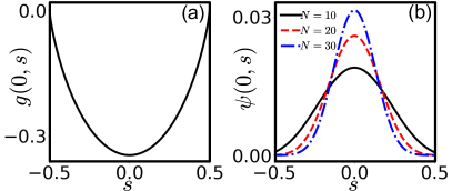
Figure S1: (a) Logarithmic wave function at $t=0$. (b) Initial wave function plotted for different values of $N$.

In the Dicke basis, the initial wave function is $\psi(0,s)=\braket{s}{\psi_{0}}\propto\sqrt{C^{n}_{N}}$. Here, we omit any constant factors that are independent of $s$ since the wave function will eventually be normalized at the final time step. Therefore, considering such factors during intermediate steps is unnecessary. Since $\ket{s}$ is an eigenstate of $\hat{V}$ with the eigenvalue $\sqrt{\gamma}2Ns$, we have

$$\bra{s}e^{-id\hat{H}_{t}}=\bra{s}e^{\hat{V}dW_{t}}=\bra{s}e^{2Ns\sqrt{\gamma}dW_{t}}.$$ (S5)

Thus, the wave function at arbitrary time $t$ can be computed as: $\psi(t,s)\propto\phi(t,s)\propto e^{2Ns\sqrt{\gamma}W_{t}}\psi(0,s)$. Next, we analyze the shape of the wave function in $s$-space. Note that $\psi(t,s)$ is real and positive.

The initial wave function reads

$$\psi(0,s)\propto\sqrt{\frac{N!}{\left[N(\frac{1}{2}+s)\right]!\left[N(\frac{1}{2}-s)\right]!}}.$$ (S6)

We are primarily interested in the case where $N$ is sufficiently large. In fact, taking the limit as $N\to\infty$ is essential in studying spontaneous symmetry breaking (SSB). Here, we assume $N$ is large enough to apply Stirling’s approximation. Using Stirling’s formula, we find:

$$\begin{split}\psi(0,s)\propto\ {\left[\left(\frac{1}{2}+s\right)^{\frac{1}{2}+s}\left(\frac{1}{2}-s\right)^{\frac{1}{2}-s}\right]^{-\frac{N}{2}}\left[{2\pi N\left(\frac{1}{4}-s^{2}\right)}\right]^{-\frac{1}{4}}}.\end{split}$$ (S7)

From this, it is easy to see that the right-hand side of Eq. (S7) increases exponentially with $N$. Thus, without loss of generality, we set $\psi(0,s)\equiv\exp\left\{-Ng(0,s)\right\}$, where $g$ is called the logarithmic wave function. It is straightforward to obtain

$$g(0,s)=\frac{1}{2}\left[\left(\frac{1}{2}+s\right)\ln\left(\frac{1}{2}+s\right)+\left(\frac{1}{2}-s\right)\ln\left(\frac{1}{2}-s\right)\right],$$ (S8)

where we have neglected the $s$-independent constant. In Fig. S1(a), we plot $g(0,s)$ as a function of $s$. It is clear that $g$ has a unique minimum. Consequently, we expect $\psi(0,s)=\exp(-Ng(0,s))$ to exhibit a single-peak structure, with a peak width on the order of $\sim 1/\sqrt{N}$. As $N$ increases, the peak becomes sharper. This is confirmed in Fig. S1(b), where plots of normalized $\psi(0,s)$ for different values of $N$ are compared. In the limit $N\to\infty$, $\psi(0,s)$ approaches a $\delta$-function.

For $t>0$, the wave function in $s$-space can be written as

$$\begin{split}\psi(t,s)\propto\ e^{2\sqrt{\gamma}NW_{t}s}{\left[\left(\frac{1}{2}+s\right)^{\frac{1}{2}+s}\left(\frac{1}{2}-s\right)^{\frac{1}{2}-s}\right]^{-\frac{N}{2}}\left[{2\pi N\left(\frac{1}{4}-s^{2}\right)}\right]^{-\frac{1}{4}}}.\end{split}$$ (S9)

Once again, the right-hand side of Eq. (S9) increases exponentially with $N$. We therefore set $\psi(t,s)\equiv\exp\left\{-Ng(t,s)\right\}$. For sufficiently large $N$, we obtain

$$g(t,s)=-\frac{1}{N}\ln\psi(t,s)=\frac{1}{2}\left[\left({\frac{1}{2}+s}\right)\ln\left(\frac{1}{2}+s\right)+\left({\frac{1}{2}-s}\right)\ln\left(\frac{1}{2}-s\right)\right]-2\sqrt{\gamma}sW_{t}.$$ (S10)

For $t>0$, according to Eq. (S10), the curve for $g(t,s)$ can be viewed as the sum of $g(0,s)$ and a straight line with slope $-4\sqrt{\gamma}W_{t}$. Adding this straight line to Fig. S1(a) simply shifts the minimum point to the left if $W_{t}>0$ or to the right if $W_{t}<0$, while the overall shape of $g$ remains the same. As a result, the peak structure of $\psi(t,s)$ is preserved.

To determine the peak location of $\psi(t,s)$, denoted by $\bar{s}$, it is equivalent to find the minimum of $g(t,s)$ along the $s$-axis. Solving the equation $\frac{\partial g}{\partial s}\left|{}_{s=\bar{s}}\right.=0$, we easily obtain

$$\bar{s}=\frac{1}{2}\tanh\left(\tilde{W}_{t}\right),$$ (S11)

where $\tilde{W}_{t}=2\sqrt{\gamma}W_{t}$, and $W_{t}$ is a random variable (Wiener process) with a Gaussian distribution of zero mean and variance $t$. From Eq. (S11) and probability theory, the distribution of the random variable $\bar{s}$ can be derived. The probability density is given by

$$P(\bar{s})=\frac{1}{1-4\bar{s}^{2}}\frac{1}{\sqrt{2\pi\gamma t}}\exp\left\{-\frac{1}{32\gamma t}\left(\ln\frac{1+2\bar{s}}{1-2\bar{s}}\right)^{2}\right\}.$$ (S12)

Similarly, we can derive the probability density of $\bar{m}=\ln\frac{1+2\bar{s}}{1-2\bar{s}}$, which is $P(\bar{m})=\frac{1}{\sqrt{32\pi\gamma t}}\exp\left({-\frac{\bar{m}^{2}}{32\gamma t}}\right)$, where $\bar{m}$ represents the rescaled magnetization.

At the initial time, the probability of finding $\bar{s}=0$ is $1$. In the limit $t\to\infty$, the probabilities of $\bar{s}=\pm 1/2$ become $50\%$ each. This behavior can be understood from the equation $\bar{s}=\frac{1}{2}\tanh\left(\tilde{W}_{t}\right)$, where the variance of $\tilde{W}_{t}$, equal to $4\gamma t$, diverges as $t\to\infty$. This means the probability of finding $\tilde{W}_{t}$ within any finite interval around zero (e.g., $\left(\tanh^{-1}\left(-1+\epsilon\right),\tanh^{-1}\left(1-\epsilon\right)\right)$) approaches zero. Here, $\epsilon$ denotes an arbitrarily small positive number, and $\tanh^{-1}$ is the inverse hyperbolic tangent function. As a result, the probability of $\bar{s}$ lying within $\left(-\frac{1}{2}+\frac{\epsilon}{2},\frac{1}{2}-\frac{\epsilon}{2}\right)$ also goes to zero for any $\epsilon>0$. Thus, in the limit, $\bar{s}$ can only take the values $\pm 1/2$.

S-3 Stochastic semiclassical approach

In this section, we consider the Hamiltonian $\hat{H}_{0}=-\frac{J}{N}\hat{\sigma}_{z}^{2}+h\hat{\sigma}_{x}$ and $\hat{V}=\sqrt{\gamma}\hat{\sigma}_{z}$, and proceed to solve Eq. (S1) to obtain the prenormalized wave function using the stochastic semiclassical approach. Normalizing $\ket{\phi_{t}}$ is straightforward and, in fact, unnecessary, as we are only interested in the wave function’s properties that are independent of its normalization.

The prenormalized state vector satisfies: $\ket{d\phi_{t}}=-i\hat{H}_{0}dt\ket{\phi_{t}}+\sqrt{\gamma}\hat{\sigma}_{z}dW_{t}\ket{\phi_{t}}+\frac{1}{2}\gamma\hat{\sigma}_{z}^{2}dt\ket{\phi_{t}}$. Using the Dicke basis, the dynamical equation for the prenormalized wave function becomes:

$$\begin{split}d_{t}\phi(t,s)=idt\ 4s^{2}JN\phi(t,s)-idt\ N\tilde{f}(s)\cosh\left(\frac{1}{N}\partial_{s}\right)\phi(t,s)+\left[2s\sqrt{\gamma}NdW_{t}+2s^{2}\gamma N^{2}dt\right]\phi(t,s),\end{split}$$ (S13)

where $\tilde{f}(s)=2h\sqrt{\frac{1}{4}-s^{2}}$ and $d_{t}\phi(t,s)\equiv\phi(t+dt,s)-\phi(t,s)$. Note that $d_{t}\phi$ is not the total differential, but rather the change in $\phi$ as $t$ changes, with $s$ held fixed. It reduces to $dt\partial_{t}\phi$ in the absence of the Wiener process. To derive Eq. (S13), we have applied the continuum approximation for the variable $s$, a standard technique for fully-connected models in the large $N$ limit Sciolla11app . In the following, we first discuss the exact solution in the specific case where $h=0$, and then explore the semiclassical method for $h\neq 0$.

S-3.1 Exact solution as $h=0$

When $h=0$ but $\gamma,J\neq 0$, the exact solution for $\phi(t,s)$ can be obtained since $\ket{s}$ is an eigenstate of $\hat{\sigma}_{z}$, which simplifies the evolution under $d\hat{H}_{t}$. Similar to the approach in Sec. S-2, the prenormalized wave function is given by:

$$\begin{split}\phi(t,s)=&\ \bra{s}\exp\left\{it\frac{J}{N}\hat{\sigma}_{z}^{2}+\sqrt{\gamma}\hat{\sigma}_{z}W_{t}\right\}\ket{\psi_{0}}\\ =&\ \exp\left\{i4Js^{2}Nt+2Ns\sqrt{\gamma}W_{t}\right\}\psi(0,s).\end{split}$$ (S14)

We can rewrite the wave function as $\phi(t,s)=\exp\left\{-Nw(t,s)\right\}$, where $w$ is the logarithmic wave function, a complex-valued function that can be split into its real and imaginary components as $w(t,s)=g(t,s)-i\theta(t,s)$. Using Eqs. (S7), (S8), and (S14), we find

$$\begin{split}&g(t,s)=g(0,s)-2\sqrt{\gamma}sW_{t},\\ &\theta(t,s)=4Jts^{2}.\end{split}$$ (S15)

Compared to the exact solution when $J=0$, a finite $J$ introduces a nonzero $\theta$, but does not affect $g$. This exact solution for $h=0$ serves as the foundation for the semiclassical approximation discussed in the following sections.

S-3.2 Semiclassical approximation as $h\neq 0$

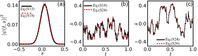
Figure S2: Comparison between the precise numerical solution and solutions from various approximation schemes. The parameters are set to $J=0.1$, $h=0.2$, and $\gamma=1$. (a) Wave function for $N=30$ and $t=0.1$: The black solid line represents the solution obtained by directly evolving the original dynamical equation for the wave function (Eq. (S13)), while the red dotted line shows the result from integrating Eq. (S18). Note the distinct deviation of the peak location from the origin, indicating $\bar{s}\neq 0$. (b) Trajectory of $\bar{s}(t)$: The black solid line is derived from solving Eq. (S18) and determining the minimum of the wave function, while the red dotted line corresponds to the solution of Eq. (S24). (c) Trajectory of $\bar{s}(t)$: The black solid line represents the solution to Eq. (S24), whereas the red dotted line corresponds to the first-order perturbation solution from Eq. (S26). Note that the stochastic dynamics were simulated using a random number generator, so the results will vary with each run of the program.

As $h\neq 0$, we develop the stochastic semiclassical approach, which relies on the fact that the wave function (whether prenormalized or normalized) exhibits a single-peak structure in $s$-space, with a peak width of approximately $1/\sqrt{N}$. As a result, instead of solving for the entire wave function, we focus on identifying the position of the peak. The stochastic semiclassical method systematically derives the equation governing the peak’s position. First, we substitute $\phi\equiv e^{-Nw}$ into Eq. (S13). Using the approximation

$$\left(\frac{1}{N}\partial_{s}\right)^{n}e^{-Nw(t,s)}=e^{-Nw(t,s)}\left[\left(-\partial_{s}w\right)^{n}+\mathcal{O}(\frac{1}{N})\right],$$ (S16)

and neglecting the $\mathcal{O}(\frac{1}{N})$ terms, we obtain the following equation for the logarithmic wave function $w$:

$$d_{t}w=idt\ \tilde{f}(s)\cosh(\partial_{s}w)-idt\ 4s^{2}J-2s\sqrt{\gamma}dW_{t}.$$ (S17)

By decomposing $w$ into its real and imaginary parts, $w(t,s)=g(t,s)-i\theta(t,s)$, we find that Eq. (S17) becomes equivalent to

$$\begin{split}&d_{t}g=dt\tilde{f}\sin(\partial_{s}\theta)\sinh(\partial_{s}g)-2s\sqrt{\gamma}\ {dW_{t}},\\ &d_{t}\theta=-dt\tilde{f}\cos(\partial_{s}\theta)\cosh(\partial_{s}g)+dt\ 4s^{2}J.\end{split}$$ (S18)

From Eq. (S13) to Eq. (S18), we neglect the $\mathcal{O}(\frac{1}{N})$ terms, a valid approximation for large $N$, as demonstrated in previous studies where $\gamma=0$ Sciolla11app , i.e., in the absence of randomness and nonHermiticity. To verify the validity of Eq. (S18) for $\gamma\neq 0$, we numerically solve the original equation, Eq. (S13), and compare its solution with Eq. (S18). Figure S2(a) shows the comparison for $N=30$, where the two solutions are nearly indistinguishable, indicating that $N=30$ is sufficiently large for Eq. (S18) to be accurate.

To solve Eq. (S18), we note that $\left|\phi\right|=e^{-Ng}$ has a single-peak structure, implying that $g$ must have a unique minimum in $s$-space (see Fig. S1(a) for $g(0,s)$). We denote this minimum point as $\bar{s}$, which corresponds to the peak position of $\left|\phi\right|$ and varies with time. Around $\bar{s}(t)$, we can expand $g(t,s)$ and $\theta(t,s)$ into Taylor’s series:

$$\begin{split}&g(t,s)=g_{0}(t)+\frac{1}{2!}g_{2}(t)\left[s-\bar{s}(t)\right]^{2}+\cdots+\frac{1}{n!}g_{n}(t)\left[s-\bar{s}(t)\right]^{n}+\cdots,\\ &\theta(t,s)=\theta_{0}(t)+\theta_{1}(t)\left[s-\bar{s}(t)\right]+\cdots+\frac{1}{n!}\theta_{n}(t)\left[s-\bar{s}(t)\right]^{n}+\cdots.\end{split}$$ (S19)

Since $\partial_{s}g=0$ at $s=\bar{s}$, there is no first-order term in the expansion of $g$. Meanwhile, $\theta_{1}(t)=\left.\partial_{s}\theta(t,s)\right|_{s=\bar{s}}$, often referred to as the classical momentum and denoted as $\bar{p}(t)$ in semiclassical literature. Using the expansion in Eq. (LABEL:eq:m:semi:gtset), we derive the differential equations for $g$ and $\theta$ as functions of time, while keeping $s$ fixed:

$$\begin{split}d_{t}g=&\ \left\{d{g}_{0}+\frac{1}{2}g_{2}\left(d\bar{s}\right)^{2}\right\}+\left\{-g_{2}d\bar{s}-dg_{2}d\bar{s}+\frac{1}{2}g_{3}\left(d\bar{s}\right)^{2}\right\}\left[s-\bar{s}\right]+\cdots\\ &+\left\{\frac{1}{n!}dg_{n}-\frac{1}{n!}g_{n+1}d\bar{s}-\frac{1}{n!}dg_{n+1}d\bar{s}+\frac{1}{n!}\frac{1}{2}g_{n+2}\left(d\bar{s}\right)^{2}\right\}\left[s-\bar{s}\right]^{n}+\cdots,\\ d_{t}\theta=&\ \left\{d\theta_{0}-\theta_{1}d\bar{s}-d\theta_{1}d\bar{s}+\frac{1}{2}\theta_{2}\left(d\bar{s}\right)^{2}\right\}+\left\{d\theta_{1}-\theta_{2}d\bar{s}-d\theta_{2}d\bar{s}+\frac{1}{2}\theta_{3}\left(d\bar{s}\right)^{2}\right\}\left[s-\bar{s}\right]+\cdots\\ &+\left\{\frac{1}{n!}d\theta_{n}-\frac{1}{n!}\theta_{n+1}d\bar{s}-\frac{1}{n!}d\theta_{n+1}d\bar{s}+\frac{1}{n!}\frac{1}{2}\theta_{n+2}\left(d\bar{s}\right)^{2}\right\}\left[s-\bar{s}\right]^{n}+\cdots.\end{split}$$ (S20)

Substituting these into the left-hand side of Eq. (S18) and similarly expanding the right-hand side, we arrive at a series of equations for $\bar{s}$, $\bar{p}$, $g_{n}$ and $\theta_{n}$. The first-order expansion yields the critical equation:

$$\begin{split}-g_{2}d\bar{s}-dg_{2}d\bar{s}+\frac{1}{2}g_{3}\left(d\bar{s}\right)^{2}=&\ dt\tilde{f}_{0}g_{2}\sin(\bar{p})-2\sqrt{\gamma}dW_{t},\\ -d\bar{p}+\theta_{2}d\bar{s}+d\theta_{2}d\bar{s}-\frac{1}{2}\theta_{3}\left(d\bar{s}\right)^{2}=&\ dt\left\{\tilde{f}_{1}\cos(\bar{p})-\tilde{f}_{0}\theta_{2}\sin(\bar{p})\right\}-dt8J\bar{s},\end{split}$$ (S21)

where the Taylor’s coefficients $\tilde{f}_{n}$ for $\tilde{f}(s)$ around $s=\bar{s}$ are given by:

$$\begin{split}\tilde{f}_{0}=2h\sqrt{\frac{1}{4}-\bar{s}^{2}},\ \ \tilde{f}_{1}=\frac{-2h\bar{s}}{\sqrt{\frac{1}{4}-\bar{s}^{2}}},\ \ \tilde{f}_{2}=-\frac{h}{2}\frac{1}{{\sqrt{\frac{1}{4}-\bar{s}^{2}}}^{3}}.\end{split}$$ (S22)

This system allows us to compute the peak position of the wave function. In the limit $N\to\infty$, the wave packet shrinks to a $\delta$-function, making the peak position the most significant feature of $\phi$. Other features become negligible for sufficiently large $N$.

Equation (S21) contains several unknown Taylor coefficients, namely $g_{2}$, $g_{3}$, $\theta_{2}$ and $\theta_{3}$. When $\gamma=0$, these unknowns cancel each other out, leading to self-consistent equations for $\bar{s}$ and $\bar{p}$. This explains why the semiclassical theory becomes exact as $N\to\infty$ in models with Hermitian Hamiltonians. However, when nonHermiticity is present (i.e., $\gamma\neq 0$), such cancellations do not occur. Moreover, including higher-order terms in the expansion does not resolve the issue, as no self-consistent set of equations for $\bar{s}$, $\bar{p}$, $g_{n}$ and $\theta_{n}$ can be obtained at any order of truncation.

To overcome this problem, we use the exact solution for $h=0$ (see Sec. S-3.1), where the transverse field is absent. For $J,\gamma\neq 0$ but $h=0$, we can already obtain the exact expression for the wave function $\phi$ as well as the logarithmic functions $g(t,s)$ and $\theta(t,s)$. Using their expressions in Eq. (S15), we can compute the corresponding Taylor series, with the coefficients given by

$$\begin{split}g_{2}(t)=\frac{2}{1-\tanh^{2}\left(\tilde{W}_{t}\right)},\ \ g_{3}(t)=\frac{8\tanh\left(\tilde{W}_{t}\right)}{\left[1-\tanh^{2}\left(\tilde{W}_{t}\right)\right]^{2}},\ \ \theta_{2}=8Jt,\ \ \theta_{3}=0,\end{split}$$ (S23)

where we have used the notation $\tilde{W}_{t}=\sqrt{\gamma}2W_{t}$. Next, we consider the case where $h$ is small but nonzero. We approximate that the expressions for $g_{n}$ and $\theta_{n}$ obtained for $h=0$ remain valid for small values of $h$. Substituting Eq. (S23) into Eq. (S21), and applying techniques from stochastic calculus, we simplify the equations for $\bar{s}$ and $\bar{p}$ as follows:

$$\begin{split}&d\bar{s}=d\left(\frac{1}{2}\tanh\left(\tilde{W}_{t}\right)\right)-2h\sqrt{\frac{1}{4}-\bar{s}^{2}}\sin\left(\bar{p}\right)dt,\\ &d\bar{p}=2h\frac{\bar{s}}{\sqrt{\frac{1}{4}-\bar{s}^{2}}}\cos(\bar{p})dt+4Jtd\left(\tanh\left(\tilde{W}_{t}\right)\right)+8J\bar{s}dt.\end{split}$$ (S24)

Note that Eq. (S24) describes a non-Markovian process. This is because $d\left(\tanh\left(\tilde{W}_{t}\right)\right)$ differs from $d{W}_{t}$; while the latter is, by definition, a random variable independent of previous values due to the independent increment property of the Wiener process, $d\left(\tanh\left(\tilde{W}_{t}\right)\right)$ depends on $\tanh\left(\tilde{W}_{t}\right)$, which is influenced by the history of increments ($dW_{t}$) before time $t$. Consequently, no Fokker-Planck equation can be derived for Eq. (S24) due to its non-Markovian nature.

To validate the use of $g_{n}$ and $\theta_{n}$ for $h=0$, we numerically solve Eq. (S18) (which has already been shown to be effective) and locate the minimum point of $g$ in $s$-space. The corresponding trajectory of the minimum point is shown as the black solid line in Fig. S2(b). For comparison, we also numerically evolve Eq. (S24) to obtain $\bar{s}(t)$, which is plotted as red dots. The excellent agreement between the two indicates that our approximation works well for small values of $h$, such as $h=0.2$.

In addition to the numerical solution, we can also solve Eq. (S24) analytically using perturbation theory, expressing the solution as a power series in $h$. The zeroth-order solution, obtained by setting $h=0$, is given by:

$$\begin{split}\bar{s}^{(0)}(t)=&\ \frac{1}{2}\tanh\left(\tilde{W}_{t}\right),\\ \bar{p}^{(0)}(t)=&\ 4Jt\tanh\left(\tilde{W}_{t}\right).\end{split}$$ (S25)

Substituting Eq. (S25) into the right-hand side of Eq. (S24) and integrating over $t$, we can obtain the first-order solution for $\bar{s}$ and $\bar{p}$, which reads:

$$\begin{split}&\bar{s}(t)\approx\frac{1}{2}\tanh\left(\tilde{W}_{t}\right)-h\int^{t}_{0}d\tau\sqrt{1-\tanh^{2}\left(\tilde{W}_{\tau}\right)}\sin\left(4J\tau\tanh\left(\tilde{W}_{\tau}\right)\right),\\ &\bar{p}(t)\approx 4Jt\tanh\left(\tilde{W}_{t}\right)+2h\int^{t}_{0}d\tau\frac{\tanh\left(\tilde{W}_{\tau}\right)}{\sqrt{1-\tanh^{2}\left(\tilde{W}_{\tau}\right)}}\cos\left(4J\tau\tanh\left(\tilde{W}_{\tau}\right)\right).\end{split}$$ (S26)

This process can be continued to obtain the solution to any order in $h$. In practice, we find the first-order solution is sufficiently accurate for the parameter range we are interested in. In Fig. S2(c), we compare the solution for $\bar{s}(t)$ obtained from directly evolving Eq. (S24) with the first-order solution from Eq. (S26). The excellent agreement demonstrates the validity of the first-order solution.

S-4 Real-time dynamics of $\bar{s}$

In the previous section, we used the stochastic semiclassical approach to solve the dynamical equation of the wave function and determine its peak position, $\bar{s}$. We demonstrated that the solution in Eq. (S26) provides a good approximation. Next, we will examine the real-time dynamics of $\bar{s}$ using Eq. (S26).

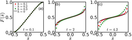
Figure S3: Cumulant distribution functions $F(\bar{s})$ at (a) $t=0.1$, (b) $t=2$, and (c) $t=4.2$. The parameter $J$ is set to 0.1. Results for different values of $h$ are represented using lines and dots of varying types and colors. Each distribution is based on $10^{4}$ samples to ensure statistical accuracy.

Recall that $\tilde{W}_{\tau}=2\sqrt{\gamma}W_{\tau}$ ($0\leq\tau\leq t$) is a random variable, and the properties of $W_{\tau}$ are well-studied in stochastic calculus. In numerical simulations, $W_{\tau}$ can be generated using $W_{\tau}=\Delta W_{t_{0}}+\Delta W_{t_{1}}+\cdots+\Delta W_{t_{n-1}}$, where $\tau=n\Delta t$ and $\Delta t$ is the time step, chosen to be sufficiently small. The terms $\Delta W_{t_{j}}$, with $j=0,1,\cdots,n-1$, are independent Gaussian random variables, each with a mean of zero and a variance of $\Delta t$. For a given time $t$, the stochastic process $W_{\tau}$ over $0\leq\tau\leq t$ is not repeatable in each simulation. Since $\bar{s}$ is expressed in terms of $\tilde{W}_{\tau}$, it is also not repeatable. Therefore, we need to repeat the simulation multiple times to capture the statistical properties, such as the cumulant distribution of the random variable $\bar{s}$. In practice, we find that $10^{4}$ samples are sufficient to achieve statistical convergence.

Figure S3 shows the cumulant distribution function of $\bar{s}$ at various times and for different values of $h$, with $J=0.1$ fixed. The exact solution for $h=0$ is also plotted for comparison. At early times (e.g., $t=0.1$), the distribution for finite $h$ ($h=0.1$, $0.2$, or $0.3$) shows no significant deviation from the distribution at $h=0$. However, as time increases, the deviation gradually becomes noticeable, with the extent of deviation depending on the value of $h$. By $t=2$, $F(\bar{s})$ for $h=0.3$ shows a clear deviation from the exact solution (see the green stars in Fig. S3(b)), but $F(\bar{s})$ for $h=0.1$ remains close to the exact solution, indicating that the deviation appears earlier as $h$ increases. At a later time ($t=4.2$), the deviations for $h=0.1$, $0.2$, and $0.3$ become more pronounced, with the magnitude of deviation increasing with $h$. At the same time, we observe that the slope of $F(\bar{s})$ near $\bar{s}=0$ decreases with time, and the deviation from the exact solution causes the slope to decrease more gradually. Since the slope of $F(\bar{s})$ represents the probability density, we conclude that the probability migration from $\bar{s}=0$ to $\bar{s}=\pm 1/2$ slows down as $h$ increases. In other words, the transverse field slows the probability migration.

S-5 Steady-state distribution of $\bar{s}$

In the previous section, we discussed the evolution of the distribution of $\bar{s}$ using the first-order perturbative solution in Eq. (S26). However, Eq. (S26) is valid only for short to intermediate times. If $t$ becomes too large, the equation may result in nonphysical values of $\left|\bar{s}\right|>1/2$. As $t\to\infty$, we expect the distribution of $\bar{s}$ to relax into a steady state. For $h=0$, this steady state corresponds to $\bar{s}=\pm 1/2$, with each value having a probability of 50%. For $h>0$, we must revisit the nonlinear stochastic equation (S24) to explore the steady-state distribution.

In Eq. (S24), as $t\to\infty$, the variance of $\tilde{W}_{t}$, which is $4\gamma t$, diverges. From probability theory, it is clear that $\tanh(\tilde{W}_{t})\to\pm 1$ in this limit. More precisely, the random variable $\tanh(\tilde{W}_{t})$ approaches $\pm 1$ with 100% probability, and the probability of it taking a value within the interval $(-1+\epsilon,1-\epsilon)$, for any arbitrarily small $\epsilon>0$, becomes zero as $t\to\infty$. Since $\tanh(\tilde{W}_{t})\to\pm 1$, we also have $d(\tanh(\tilde{W}_{t}))\to 0$ with 100% probability. Thus, the dynamical equations (S24) reduce to

$$\begin{split}&d\bar{s}=-2h\sqrt{\frac{1}{4}-\bar{s}^{2}}\sin\left(\bar{p}\right)dt,\\ &d\bar{p}=2h\frac{\bar{s}}{\sqrt{\frac{1}{4}-\bar{s}^{2}}}\cos(\bar{p})dt+8J\bar{s}dt.\end{split}$$ (S27)

In the limit $t\to\infty$, only the terms involving $J$ and $h$ remain, while the terms related to $\gamma$ vanish. This indicates that the non-Hermitian random part of the Hamiltonian loses its influence on $\bar{s}$, the peak position of the wave function.

Equation (LABEL:eq:m:ste:dsdp) is identical to the one found in the semiclassical theory of the transverse-field Ising model Sciolla11app . This can also be seen within our stochastic semiclassical approach by setting $\gamma=0$ in Eq. (S21). With $\gamma=0$, the random terms involving $dW_{t}$ are removed from Eq. (S21), and the second-order differentials disappear, as all the first-order differentials are now proportional to $dt$. As a result, the terms $g_{n}$ and $\theta_{n}$ in Eq. (S21) cancel each other, leading to the emergence of Eq (LABEL:eq:m:ste:dsdp). If we consider the quantum dynamics governed by the Hermitian Hamiltonian $\hat{H}_{0}=-\frac{J}{N}\hat{\sigma}_{z}^{2}+h\hat{\sigma}_{x}$, with the initial state having all spins aligned along the positive $x$-direction, the quantities $\bar{s}$ and $\bar{p}$ obtained from the wave packet strictly satisfies Eq. (LABEL:eq:m:ste:dsdp).

Figure S4: Equal-energy contours in the $\bar{s}-\bar{p}$ plane, governed by the classical dynamics described by the Hamiltonian $H(\bar{s},\bar{p})=2h\sqrt{\frac{1}{4}-\bar{s}^{2}}\cos\bar{p}-4J\bar{s}^{2}$. Arrows indicate the direction of motion along the contours. Parameters are set to $h=0.2$ and $J=0.1$.

Moreover, Eq. (LABEL:eq:m:ste:dsdp) describes the motion of a classical point in the $\bar{s}-\bar{p}$ plane, governed by classical Hamiltonian equations: $d\bar{p}/dt=\partial H/\partial\bar{s}$ and $d\bar{s}/dt=-\partial H/\partial\bar{p}$, where the Hamiltonian is given by $H(\bar{s},\bar{p})=2h\sqrt{\frac{1}{4}-\bar{s}^{2}}\cos\bar{p}-4J\bar{s}^{2}$. The Hamiltonian $H$ is conserved, remaining invariant throughout the system’s evolution. In Fig. S4, we show an example of constant $H$ contours (equal-$H$ lines) in the $\bar{s}-\bar{p}$ plane, with parameters set to $h=0.2$ and $J=0.1$. The arrows indicate the direction of motion for the point $\left(\bar{s},\bar{p}\right)$ along these contours. In the $\bar{s}-\bar{p}$ plane, $d\bar{s}/dt$ and $d\bar{p}/dt$ can be interpreted as the velocity of a fluid. This allows us to derive a corresponding Fokker-Planck equation, as the dynamics described by Eq. (LABEL:eq:m:ste:dsdp) now represent a Markovian process, with the nonMarkovian terms such as $d\tanh\left(\tilde{W}_{t}\right)$ having been neglected. The Fokker-Planck equation is given by:

$$\begin{split}\partial_{t}P(\bar{s},\bar{p},t)=\partial_{\bar{s}}\left[2h\sqrt{\frac{1}{4}-\bar{s}^{2}}\sin\left(\bar{p}\right)\cdot P(\bar{s},\bar{p},t)\right]-\partial_{\bar{p}}\left[\left(2h\frac{\bar{s}}{\sqrt{\frac{1}{4}-\bar{s}^{2}}}\cos(\bar{p})+8J\bar{s}\right)\cdot P(\bar{s},\bar{p},t)\right].\end{split}$$ (S28)

References

- (1) G. C. Ghirardi, A. Rimini, and T. Weber, Phys. Rev. D 34, 470 (1986).
- (2) L. Diósi, Phys. Rev. A 40, 1165 (1989).
- (3) A. Bassi, J. Phys. A 38, 3173 (2005).
- (4) P. Pearle, Phys. Rev. A 39, 2277 (1989).
- (5) G. C. Ghirardi, P. Pearle, and A. Rimini, Phys. Rev. A 42, 78 (1990).
- (6) R. Penrose, Gen. Relativ. Gravit. 28, 581 (1996).
- (7) P. Pearle, Phys. Rev. A 59, 80 (1999).
- (8) S. L. Adler and A. Bassi, J. Phys. A 40, 15083 (2007).
- (9) S. L. Adler and A. Bassi, J. Phys. A 41, 395308 (2008).
- (10) A. Bassi, K. Lochan, S. Satin, T. P. Singh, and H. Ulbricht, Rev. Mod. Phys. 85, 471 (2013).
- (11) A. Vinante, M. Bahrami, A. Bassi, O. Usenko, G. Wijts, and T. H. Oosterkamp, Phys. Rev. Lett. 116, 090402 (2016).
- (12) A. Vinante, R. Mezzena, P. Falferi, M. Carlesso, and A. Bassi, Phys. Rev. Lett. 119, 110401 (2017).
- (13) M. Bahrami, Phys. Rev. A 97, 052118 (2018).
- (14) A. Tilloy and T. M. Stace, Phys. Rev. Lett. 123, 080402 (2019).
- (15) A. Pontin, N. P. Bullier, M. Toroš, and P. F. Barker, Phys. Rev. Res. 2, 023349 (2020).
- (16) A. Vinante, M. Carlesso, A. Bassi, A. Chiasera, S. Varas, P. Falferi, B. Margesin, R. Mezzena, and H. Ulbricht, Phys. Rev. Lett. 125, 100404 (2020).
- (17) D. Zheng, Y. Leng, X. Kong, R. Li, Z. Wang, X. Luo, J. Zhao, C.-K. Duan, P. Huang, J. Du, M. Carlesso, and A. Bassi, Phys. Rev. Res. 2, 013057 (2020).
- (18) K. Komori, Y. Enomoto, C. P. Ooi, Y. Miyazaki, N. Matsumoto, V. Sudhir, Y. Michimura, and M. Ando, Phys. Rev. A 101, 011802(R) (2020).
- (19) S. Donadi, K. Piscicchia, C. Curceanu, L. Diósi, M. Laubenstein, and A. Bassi, Nat. Phys. 17, 74 (2021).
- (20) G. Gasbarri, A. Belenchia, M. Carlesso, S. Donadi, A. Bassi, R. Kaltenbaek, M. Paternostro, and H. Ulbricht, Commun. Phys. 4, 155 (2021).
- (21) M. Carlesso, S. Donadi, L. Ferialdi, M. Paternostro, H. Ulbricht, and A. Bassi, Nat. Phys. 18, 243 (2022).
- (22) N. Gisin and I. C. Percival, J. Phys. A: Math. Gen. 25, 5677 (1992).
- (23) I. Percival, Quantum State Diffusion (Cambridge University Press, Cambridge, 1998).
- (24) M. B. Plenio and P. L. Knight, Rev. Mod. Phys. 70, 101 (1998).
- (25) A. J. Daley, Adv. Phys. 63, 77 (2014).
- (26) Y. Castin and K. Mølmer, Phys. Rev. Lett. 74, 3772 (1995).
- (27) W. L. Power and P. L. Knight, Phys. Rev. A 53, 1052 (1996).
- (28) C. Ates, B. Olmos, J. P. Garrahan, and I. Lesanovsky, Phys. Rev. A 85, 043620 (2012).
- (29) A. Hu, T. E. Lee, and C. W. Clark, Phys. Rev. A 88, 053627 (2013).
- (30) M. Raghunandan, J. Wrachtrup, and H. Weimer, Phys. Rev. Lett. 120, 150501 (2018).
- (31) B. Pokharel, M. Z. Misplon, W. Lynn, P. Duggins, K. Hallman, D. Anderson, A. Kapulkin, and A. K. Pattanayak, Sci. Rep. 8, 2108 (2018).
- (32) H. Weimer, A. Kshetrimayum, and R. Orús, Rev. Mod. Phys. 93, 015008 (2021).
- (33) V. P. Singh and H. Weimer, Phys. Rev. Lett. 128, 200602 (2022).
- (34) W. C. Myrvold, Phys. Rev. A 96, 062116 (2017).
- (35) R. Tumulka, A Relativistic GRW Flash Process with Interaction (Springer, New York, 2020).
- (36) C. Jones, T. Guaita, and A. Bassi, Phys. Rev. A 103, 042216 (2021).
- (37) C. Jones, G. Gasbarri, and A. Bassi, J. Phys. A 54, 295306 (2021).
- (38) C. M. Bender, Rep. Prog. Phys. 70, 947 (2007).
- (39) I. Rotter, J. Phys. A: Math. Theor. 42, 153001 (2009).
- (40) N. Hatano and D. R. Nelson, Phys. Rev. Lett. 77, 570 (1996)
- (41) Y. Xiong, J. Phys. Commun. 2, 035043 (2018).
- (42) V. M. Martinez Alvarez, J. E. Barrios Vargas, and L. E. F. Foa Torres, Phys. Rev. B 97, 121401(R) (2018).
- (43) S. Yao and Z. Wang, Phys. Rev. Lett. 121, 086803 (2018).
- (44) Z. Gong, Y. Ashida, K. Kawabata, K. Takasan, S. Higashikawa, and M. Ueda, Phys. Rev. X 8, 031079 (2018).
- (45) F. K. Kunst, E. Edvardsson, J. C. Budich, and E. J. Bergholtz, Phys. Rev. Lett. 121, 026808 (2018).
- (46) K. Kawabata, K. Shiozaki, M. Ueda, and M. Sato, Phys. Rev. X 9, 041015 (2019).
- (47) J. C. Budich, J. Carlström, F. K. Kunst, and E. J. Bergholtz, Phys. Rev. B 99, 041406(R) (2019).
- (48) J. C. Budich and E. J. Bergholtz, Phys. Rev. Lett. 125, 180403 (2020).
- (49) L. Xiao, T. Deng, K. Wang, Z. Wang, W. Yi, and P. Xue, Phys. Rev. Lett. 126, 230402 (2021).
- (50) W.-T. Xue, Y.-M. Hu, F. Song, and Z. Wang, Phys. Rev. Lett. 128, 120401 (2022).
- (51) H.-Y. Wang, F. Song, and Z. Wang, Phys. Rev. X 14, 021011 (2024).
- (52) R. El-Ganainy, K. G. Makris, M. Khajavikhan, Z. H. Musslimani, S. Rotter, and D. N. Christodoulides, Nat. Phys. 14, 11 (2018).
- (53) E. J. Bergholtz, J. C. Budich, and F. K. Kunst, Rev. Mod. Phys. 93, 015005 (2021).
- (54) P. Wang, Phys. Rev. D 105, 115037 (2022).
- (55) See Supplementary Materials.
- (56) B. Sciolla and G. Biroli, J. Stat. Mech., P11003 (2011).
- (57) M Henkel, H. Hinrichsen, and S. Lübeck, Non-Equilibrium Phase Transitions (Canopus Academic Publishing Limited, 2008).

References

- (1) T. Mikosch, Elementary stochastic calculus with finance in view (World Scientific Publishing Co. Pte. Ltd., 1998).
- (2) B. Sciolla and G. Biroli, J. Stat. Mech., P11003 (2011).