Gradient Routing: Masking Gradients to Localize Computation in Neural Networks

Abstract

Neural networks are trained primarily based on their inputs and outputs, without regard for their internal mechanisms. These neglected mechanisms determine properties that are critical for safety, like (i) transparency; (ii) the absence of sensitive information or harmful capabilities; and (iii) reliable generalization of goals beyond the training distribution. To address this shortcoming, we introduce gradient routing, a training method that isolates capabilities to specific subregions of a neural network. Gradient routing applies data-dependent, weighted masks to gradients during backpropagation. These masks are supplied by the user in order to configure which parameters are updated by which data points. We show that gradient routing can be used to (1) learn representations which are partitioned in an interpretable way; (2) enable robust unlearning via ablation of a pre-specified network subregion; and (3) achieve scalable oversight of a reinforcement learner by localizing modules responsible for different behaviors. Throughout, we find that gradient routing localizes capabilities even when applied to a limited, ad-hoc subset of the data. We conclude that the approach holds promise for challenging, real-world applications where quality data are scarce.

1 Introduction

As AI systems become more powerful and more prevalent, there is an increasing need to explain and control the inner mechanisms governing their behavior. To address this challenge, some researchers aim to fully understand AI systems, either by reverse engineering the operations of conventionally trained models (Olah et al., 2020; Olsson et al., 2022) or with inherently interpretable architectures (Koh et al., 2020; Hewitt et al., 2023; Xin et al., 2022). This is not necessary. If we could understand or control the mechanisms underlying a neural network’s computation with respect to a limited set of safety-critical properties, such as hazardous information or the capacity for deception, that might be sufficient to make significant safety guarantees.

To achieve targeted control over neural network internals, we propose gradient routing, a training method for localizing capabilities to chosen subregions of a neural network. Gradient routing is a modification of backpropagation that uses data-dependent, weighted masks to control which network subregions are updated by which data points. By appropriately specifying these masks, a user can configure which parts of the network (parameters, activations, or modules) are updated by which data points (e.g. specific tokens, documents, or based on data labels). The resulting network is similar to a conventionally trained network, but with some additional internal structure.

Our contributions are as follows. In Section 2, we discuss prior work on neural network modularity, unlearning, and scalable oversight. In Section 3, we define gradient routing and comment on its practical implementation. Most of the paper is a tour of gradient routing applications:

Section 4.1

We use gradient routing to control the encodings learned by an MNIST autoencoder to split them into two halves, with each half representing different digits.

Section 4.2

We apply gradient routing to localize features in language models. First, we train a model that can be steered by a single scalar value, showing that feature localization is possible, even with narrowly-scoped labels. Next, we present Expand, Route, Ablate, an application of gradient routing that enables robust unlearning via ablation of a pre-specified network subregion. This unlearning is nearly as resistant to retraining as a gold-standard model never trained on the task. Finally, we show that this unlearning method scales to a large (0.7B) model.

Section 4.3

We apply gradient routing to the problem of scalable oversight (Amodei et al., 2016), where the aim is to train a performant policy despite limited access to reliable labels. We train a policy network by reinforcement learning to navigate to two kinds of grid squares in a toy environment, Diamond and Ghost. Using gradient routing, we localize modules responsible for these two behaviors. We show that we can steer the policy towards Diamond by ablating the Ghost module. Gradient routing trains steerable networks even when the amount of labeled training data is small, and even when the policy is able to condition on the existence of labels. As a result, our method outperforms baselines, including data filtering.

In Section 5, we discuss themes from our findings, including an observed absorption effect, where gradient routing applied to a narrow subset of data has a broader localizing effect on capabilities related to that data. Absorption provides an answer to the question: “If one has labels that are suitable for localizing undesirable computation, why not simply use those labels to filter the data?” When labels do not encompass all training data from which harmful capabilities arise, absorption means that localization can still occur, whereas filtering may be inadequate. Furthermore, localization does not explicitly influence the learned behavior of a model, a fact we exploit to achieve scalable oversight.

We conclude by noting that black-box training techniques may be inadequate for high-stakes machine learning applications. Localization techniques, like gradient routing, may provide a solution.

2 Related work

Training to localize pre-specified capabilities. Akin to gradient routing, work in modular machine learning trains modules to contain concepts or abilities determined in advance of training. Typically, modular architectures involve a routing function that selects modules to apply on a forward pass (Pfeiffer et al., 2023). Routing functions are often unsupervised, as with a typical mixture of experts setup (Jacobs et al., 1991; Eigen et al., 2013; Shazeer et al., 2017). However, some approaches route inputs based on metadata, creating modules with known specializations (Waibel & II, 1992). For example, routing has been based on (i) the modality of data in multi-modal models (Pfeiffer et al., 2021), (ii) language (Pfeiffer et al., 2020; 2022; Fan et al., 2021), and (iii) low- vs. high-level control or task type in robotics (Heess et al., 2016; Devin et al., 2017). Gururangan et al. (2021) separate the training data of a language model by domain and assign one expert in each layer to a single domain. By disabling the expert for a domain, they are able to approximate a model that was not trained on the domain.

Other methods freeze the weights of a pre-trained model and train a newly added module, with the aim of localizing the task to the new module (Rebuffi et al., 2017; 2018; Houlsby et al., 2019; Bapna & Firat, 2019). Zhang et al. (2024) locate capabilities in models by learning a weight mask, transfer the identified sub-network to a randomly initialized model, then train as if from scratch. By choosing a suitable sub-network, they can, for example, induce a vision model to identify ImageNet (Deng et al., 2009) classes by shape, not texture.

Adversarial representation learning and concept erasure. In order to control the information in learned representations, prior works have trained feature extraction networks adversarially against discriminator networks that predict this information (Goodfellow et al., 2014; Schmidhuber, 1992; Ganin & Lempitsky, 2015; Ganin et al., 2016; Edwards & Storkey, 2015). Other works have removed concepts by modifying activations during inference (Ravfogel et al., 2020; Belrose et al., 2023; Elazar et al., 2020; Bolukbasi et al., 2016).

Robust unlearning. Machine unlearning seeks to remove undesired knowledge or abilities from a pre-trained neural network (Cao & Yang, 2015; Li et al., 2024). Typical unlearning methods are brittle in the sense that the unlearned abilities of the model can be recovered by fine-tuning on a tiny number of data points (Henderson et al., 2023; Sheshadri et al., 2024; Lynch et al., 2024; Liu et al., 2024; Shi et al., 2024; Patil et al., 2023; Lo et al., 2024; Lermen et al., 2023). Lee et al. (2024); Łucki et al. (2024) suggest that undesired concepts are more easily “bypassed” than thoroughly removed from model weights. In this paper, we pre-train models with gradient routing such that we can perform robust unlearning, which cannot be easily undone by retraining. Tampering Attack Resistance (TAR) (Tamirisa et al., 2024) also targets robust unlearning in LLMs. While their method does improve robustness to retraining, it degrades general model performance as a side effect. However, we present gradient routing as a training technique rather than a post-hoc modification, so the two methods aren’t directly comparable.

Compared to gradient routing, the most similar approaches prune or mask parts of the network most important for the target behavior. SISA (Bourtoule et al., 2021) trains multiple models in parallel on partitions of the dataset and takes “votes” from each model at inference time. Similar to ablating a network subregion, a model can be dropped to achieve robust unlearning. The approach of Bayazit et al. (2023) is to learn a mask over parameters in a language model to unlearn specific facts, while Huang et al. (2024) and Pochinkov & Schoots (2024) remove neurons related to harmful behavior in order to restore the alignment of an adversarially fine-tuned language model. Guo et al. (2024) fine-tune the parameters of only the most important components for the task. Lizzo & Heck (2024) instead delete subspaces of the model parameters in order to remove specific knowledge. Unfortunately, Lo et al. (2024) find that models pruned to remove a concept can very quickly relearn the concept with further training. This may be because identifying the precise sub-network for a task post-hoc is very challenging, as evidenced by the modest success of “circuit discovery” in mechanistic interpretability thus far (Wang et al., 2023; Conmy et al., 2023; Miller et al., 2024; McGrath et al., 2023).

Scalable oversight. Scalable oversight is the problem of providing a supervised training signal for behaviors that are difficult or expensive to assess (Amodei et al., 2016). Semi-supervised reinforcement learning frames scalable oversight in terms of RL on partially labeled data (Zhu et al., 2009; Finn et al., 2016; van Engelen & Hoos, 2019). Another approach is weak-to-strong generalization, in which a less powerful model provides supervision to a more powerful one (Burns et al., 2024; Kenton et al., 2024; Radhakrishnan et al., 2023). Weak-to-strong generalization introduces a potential risk: the stronger model may exploit blind spots in the weaker model’s supervision capabilities.

3 Gradient routing controls what is learned where

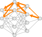
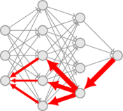
Figure 1: Gradient routing applied to three different data points. Gradient routing uses masks (shown here) to zero-out or re-weight gradients as they are backpropagated through the computational graph (denoted by arrow thickness). By supplying different masks for different data points (denoted by colors), the user controls what regions of the network learn to predict different data points.

In order to train models that are interpretable and controllable in targeted ways, we seek to localize specific knowledge or capabilities to network subregions. To do this, gradient routing applies data-dependent, weighted masks to gradients during backpropagation to configure what data (whether it be defined in terms of tokens, documents, or based on other labels) is learned where in the network (e.g. at the level of parameters, activations, or modules). The result is a model with a partially-understandable internal structure, where particular regions correspond to known capabilities. Throughout this paper, we will use “route $X$ to $Y$” to mean “use gradient routing to limit learning updates for data points $X$ to region $Y$ of the neural network.”

Let $(\mathcal{V},\mathcal{E})$ be the nodes and edges of the computational graph corresponding to a neural network and loss function, with $v(z)$ taken to be the output of node $v$ if $z$ is input to the network. Given a dataset $\mathcal{D}=\{z_{i}\}_{i=1}^{n}$, for each data point $z_{i}$, gradient routing requires the specification of a gradient route given by $\widetilde{\mathcal{E}}_{i}=\{\alpha^{i}_{e}\in\mathbb{R}:e\in\mathcal{E}\}$ and visualized in fig. 1. Define $\frac{\partial L(z)}{\partial{v}}\triangleq\frac{\partial L(\zeta)}{\partial{v}(\zeta)}|_{\zeta=z}$, the partial derivative of the loss $L$ with respect to the output of node $v$ when evaluated at input $z$. The routed derivative (denoted with a tilde) of the loss over a batch $\mathcal{B}\subseteq[n]$ is then defined recursively as $\frac{\widetilde{\partial}L(z_{i})}{\widetilde{\partial}L}\triangleq 1\text{ for all }i\in\mathcal{B}$, and

$$\frac{\widetilde{\partial}L(z_{i})}{\widetilde{\partial}v}\triangleq\sum_{u\in\mathrm{child}(v)}{\alpha^{i}_{(v,u)}}\frac{\widetilde{\partial}L(z_{i})}{\widetilde{\partial}u}\frac{\partial u(z_{i})}{\partial v},$$

for all non-terminal nodes $v\in\mathcal{V}\setminus\{L\}$ and $i\in\mathcal{B}$. Choosing $\alpha_{e}^{i}\equiv 1$ recovers standard backpropagation. This weighting is only applied in the backward pass; the forward pass is left unchanged. Any gradient-based optimizer, like SGD or Adam (Kingma, 2014), can then be used to train with these modified gradients.

It is costly to define gradient routes over every data point and edge in the computational graph. In practice, we limit masks to a small set of edges, like the outputs of specific MLP neurons or the outputs of specific layers. Also, we typically assign gradient routes to data points based on membership in a coarse partition, like the forget set or retain set in an unlearning problem. Implementation is straightforward and efficient: fig. 2 gives sample Pytorch (Paszke et al., 2019) code in which masking is applied to the outputs of sequential layers.

⬇

def forward(self, x: Tensor, gradient_masks: list[Tensor]):

for layer, mask in zip(self.layers, gradient_masks):

act = layer(x)

x = mask * act + (1 - mask) * act.detach()

return x

Figure 2: Example of gradient routing implemented in PyTorch. For each batch of training data points x, a batch of gradient_masks corresponding to those data points is passed as well. The detach() method applies the stop-gradient operator, preventing gradients from being backpropagated through act but leaving its value unchanged.

4 Applications

4.1 Routing gradients to partition MNIST representations

As a first example of feature localization via gradient routing, we train a simple MLP autoencoder on the MNIST handwritten digit dataset (LeCun et al., 1998) and use label-dependent stop-gradients to control where features for different digits are encoded. The goal is to obtain an autoencoder that reconstructs all digits (0-9) via an encoding that is made up of non-overlapping subcomponents corresponding to distinct subsets of digits. We choose subsets $\{0,1,2,3,4\}$ and $\{5,6,7,8,9\}$. To hint at the potential difficulty of this task, we note the encodings learned by an autoencoder trained on one of these sets admit low-error reconstructions on the other set, despite never being trained on it (details in appendix B).

We use a simple architecture of three-layer MLP modules with ReLU activations: an Encoder, a Decoder, and a Certificate. The Encoder processes a 28$\times$28 image into a vector in $\mathbb{R}^{32}$, and the Decoder processes that vector into a 28$\times$28 reconstruction. The Certificate is a decoder trained only on the bottom half of the encoding, which takes values in $\mathbb{R}^{16}$. Certificate updates do not affect the encoding. If the Decoder can reconstruct a digit that the Certificate cannot, this “certifies” that robust feature localization occurred (into the top half encoding, and away from the bottom half).

We use gradient routing to train an encoding split so that the top half encodes digits 0-4 and the bottom half encodes digits 5-9. While training on all digits, we apply stop-gradients to the bottom half of the encoding for digits 0-4 and stop-gradients to the top half of the encoding for digits 5-9. To induce specialization in the two halves of the encoding, we add the L1 norm of the encoding as a penalty term to the loss. The setup is shown in fig. 3(a). The results, shown in fig. 3(b) and fig. 3(c), are stark: while using the entire encoding allows the Decoder to reproduce all digits with low loss, the Certificate is only able to reproduce 5-9 from the bottom half of the encoding, as desired. Furthermore, the Certificate’s learned predictions for digits 0-4 are approximately constant. This suggests that we have successfully eliminated most information relevant to digits 0-4 from the encoding. We elaborate on experiment details and provide an extensive ablation study in appendix B.

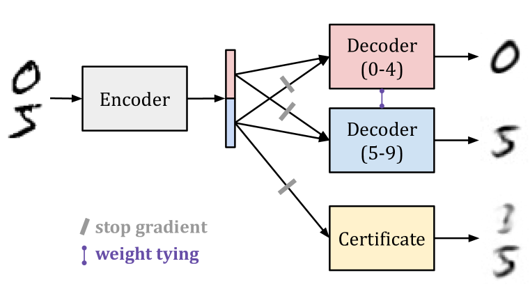
(a) An autoencoder trained to encode digits 0-4 in the top half encoding and digits 5-9 in the bottom half. The full encoding is processed by a single Decoder module trained with gradient routing; we illustrate this using weight tying. The Certificate is trained to reconstruct all digits using only the bottom half encoding.

(b) Average (across 20 runs) validation set reconstruction losses, measured as the pixel-wise mean absolute error (MAE) for the Decoder and the Certificate, demonstrating successful localization of information about digits 0-4 to the top half encoding. Run-to-run variation is negligible.

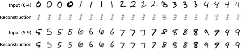
(c) Certificate reconstructions on digits from the validation set. The near-constant prediction of the Certificate on digits 0-4 illustrates the absence of information about those digits from the bottom half of the encoding.

Figure 3: Gradient routing induces a clean split in the encodings of a simple MLP autoencoder trained on MNIST digits. By applying data-dependent stop-gradients and L1 regularization, the top half of the encoding comes to represent digits 0-4 only, and the bottom half of the encoding comes to represent digits 5-9 only.

4.2 Localizing targeted capabilities in language models

In this section, we show that gradient routing applied to a small set of tokens can be used to localize broader features or capabilities in Transformer (Vaswani, 2017) language models. This is first demonstrated in terms of model activations, then applied to MLP layers for the purpose of robust unlearning.

4.2.1 Steering scalar: localizing concepts to residual stream dimensions

Elhage et al. (2021) frames the inter-block activations of a Transformer, or the residual stream, as the central communication channel of a Transformer, with all layers “reading from” and “writing into” it. Usually, the standard basis of the residual stream is indecipherable, with dimensions not corresponding to interpretable concepts. We pre-train a 303M parameter Transformer on the FineWeb-Edu dataset (Penedo et al., 2024) while routing the gradients for all _California tokens to the 0^th entry of the residual stream on layers 6-18. On token positions predicting _California, we mask gradients (to zero) on every residual stream dimension except the 0^th in layers 6-18. This masking causes the learning updates for those token positions to be localized to the weights that write into the 0^th dimension of the residual stream. After training, we look at which tokens’ unembedding vectors have the highest cosine similarity with the one hot vector for the 0^th entry of the residual stream. We find that _California has the highest cosine similarity, followed by California, _Californ, _Oregon, _Colorado, _Texas, _Florida, _Arizona, _Sacramento, and _Los; see appendix D for the top 300. These tokens all have semantic similarity to California, but gradient routing was not applied to them. This shows that gradient routing localizesbroader semantic concepts, rather than the narrow set of explicitly-routed tokens.

Past work on activation steering (Turner et al., 2023; Rimsky et al., 2024) computed (non-axis aligned) steering vectors specified by $d_{\text{model}}$ different values. However, since we localized California-related concepts to the 0^th dimension of the residual stream, we can steer the model to generate text related to California by adding a single scalar value to the 0^th entry of the residual stream during the forward pass. Appendix D provides steered model completions.

4.2.2 Gradient routing enables robust unlearning via ablation

Robust unlearning (Sheshadri et al., 2024) means training models which lack the internal mechanisms or “knowledge” required for certain tasks, as opposed to merely performing poorly on those tasks. To address this open problem, we show that gradient routing can be used to localize capabilities to a known region of the network, then delete that region, removing those capabilities.

Figure 4: Backpropagation in the Route step of Expand-Route-Ablate, showing the flow of gradients through a Transformer for tokens in the forget set. Gradients for retain tokens are unmodified. Additional dimensions, shown with dashed outlines, were added to target layers in the MLP and attention blocks, and will be removed after training in the Ablate step. All modules participate in the forward pass.

To enable comprehensive comparisons, our initial study on robust unlearning applies gradient routing to a small (28M parameter) Transformer. This model is trained on an LLM-generated dataset of simple children’s stories based on the TinyStories dataset (Eldan & Li, 2023; Janiak et al., 2024). We partition the data into: 1) a forget set made up of any story containing one of the keywords “forest(s)”, “tree(s)”, or “woodland(s)”, and 2) a retain set made up of all other stories. An example story is given in appendix C. The goal is to train a model that performs well on the retain set but poorly on the forget set, and whose forget set performance is not easily recoverable by fine-tuning. To do this, we route specific forget tokens to designated MLP neurons using three-step process termed Expand, Route, Ablate (ERA):

1. Expand

Increase the dimensionality of the model by adding randomly-initialized neurons to particular target layers.

2. Route

Train the model by supervised learning on next-token prediction, but on select tokens in forget stories, reduce the learning rate in the original dimensions of the model at the target layers. Figure 4 illustrates the routing step.

3. Ablate

Delete the additional neurons. Post-ablation, apply a very small number of steps of fine-tuning on retain data to correct for degradation caused by ablation.

Does gradient routing localize capabilities that can be robustly ablated? To answer this question, we train five types of models: an ERA model that uses gradient routing to localize forget set concepts, a base model trained conventionally on all data, a pure model trained only on retain data to serve as a gold standard, a control model trained equivalently to ERA except without gradient routing and an RMU model (Li et al., 2024) fine-tuned from the base model to serve as an unlearning baseline. Using these models, we obtain the following results. Approximate $95\%$ confidence intervals for the mean ($N=60$ runs) are given in parentheses or highlighted in figures.

• Shallow unlearning measures the degradation in forget loss caused by our method by comparing the loss on the forget set for the ERA model vs. the base model. Result: ERA achieves shallow unlearning, with forget loss of $1.91\,(\pm 0.05)$, vs. base model forget loss $1.47\,(\pm 0.02)$.

• Robust unlearning measures the robust removal of capabilities by comparing the forget loss after fine-tuning on forget data for the ERA model vs. the pure model. Figure 5(a) shows that the ERA model is almost as hard to retrain on forget data as the gold-standard pure model. In contrast, RMU’s performance is easily recovered by less than a batch of data. We comment on the choice of RMU as a baseline in appendix C.

• Alignment tax measures the cost of gradient routing in terms of retain set performance, by comparing the loss on the retain set for the ERA model vs. the base model. Result: $1.67\,(\pm 0.01)$ ERA, $1.59\,(\pm 0.01)$ base. The reduced performance of ERA is influenced by the prevalence of forget data, which constitutes 21% of the training data. In fig. 11, we show that the performance gap is negligible when the forget set constitutes as much as 5% of the training data.

• The differential effect of routing measures the impact of ablation on the ERA model vs. the control model. Figure 5(b) shows that ablation has a large effect on the control model, particularly in terms of increasing forget loss, as compared to a negligible effect on the control model.

Losses are always calculated on held-out validation data. ERA setup and experiment details are given in appendix C.

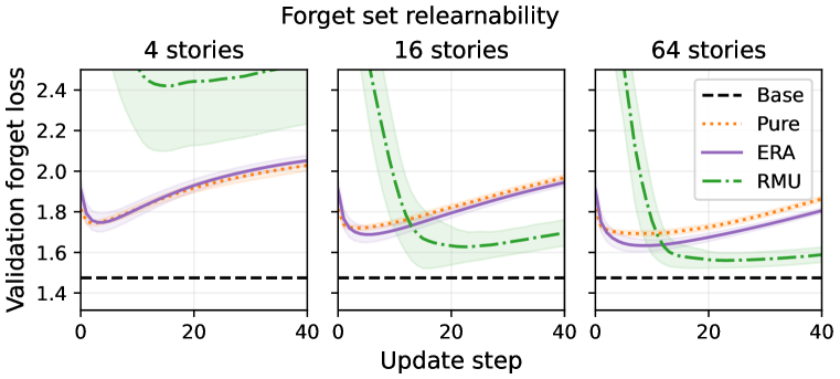
(a)

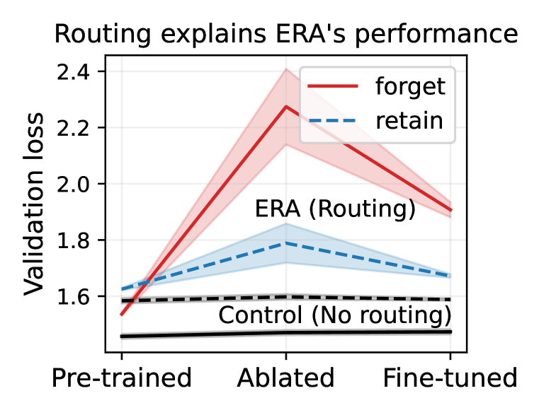
(b)

Figure 5: Gradient routing trains a language model with subcomponents that can be ablated to achieve robust unlearning. Left: (a) The average (across runs) validation forget set loss for the ERA model and pure model over 40 steps of fine-tuning on batches of varying numbers of forget data points: 4, 16, and 64. RMU is included as a foil to show the “shallowness” typical of most unlearning methods. Right: (b) Average forget and retain set validation loss after training, after ablation, and after fine-tuning for ERA vs. a control model that is exactly equivalent except gradients were not modified. Note: the $x$-axis is not to scale; pre-ablation training is on 400,000 stories, ablation is immediate, and fine-tuning is on 64 stories.

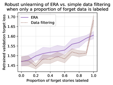
Figure 9: The performance of gradient routing vs. data filtering when a random proportion of the forget data is unlabeled, based on $N=13$ runs per setting (of model and labeling proportion). Gradient routing routes labeled data to expanded dimensions of target layers, and trains on unlabeled data as if it were in the retain set. Data filtering means the model trains on unlabeled forget data but not on labeled forget data. The “Retrained validation forget loss” refers to the lowest forget validation loss achieved when training on a batch of 64 forget tokens from the train set.

Robustness to missing labels. Finally, we show that ERA achieves robust unlearning even when only a random i.i.d. subset of forget samples are labeled, with unlabeled samples treated as retain data for training purposes. This is meant to model real-world scenarios where comprehensive labeling is infeasible. Compared against a conventionally trained model that does not train on labeled forget data, ERA achieves (on average, across runs) higher retrained validation forget loss for all labeling proportions measured besides 100%. For example, at 60% labeling, ERA achieves a retrained forget loss of 1.53 ($\pm$0.02) as opposed to 1.49 ($\pm$0.02) for the baseline. Full curves are shown in Figure 9 in Section C.1.

4.2.3 Scaling robust unlearning to larger language models

Gradient routing can localize capabilities in larger models. Motivated by the dual-use nature of AI (Urbina et al., 2022), we would like to train useful models that lack certain harmful capabilities. Here, we seek to localize and remove bioweapon-related capabilities in a 0.7B parameter Transformer. To do this, we route 20 tokens related to virology to the 0^th through 79^th MLP dimensions on layers 0 through 7 of the Transformer. Appendix E provides further details on the model and training.

Table 1 evaluates the model on a validation split of regular FineWeb-Edu data and on some of the WMDP-bio (Li et al., 2024) forget set. Ablating the target region of the network increases loss greatly on both datasets. We then fine-tune the model on a train split of FineWeb-Edu for 32 steps to restore some performance. Finally, we retrain for twenty steps on a separate split of two WMDP-bio forget set datapoints, as Sheshadri et al. (2024) do, and report the lowest loss on the validation split of the WMDP-bio forget set.

The results are striking: even after retraining on virology data, loss increases much more on the WMDP-bio forget set (+0.182) than on FineWeb-Edu (+0.032), demonstrating successful localization and robust removal of virology capabilities. A natural concern would be that ablation merely decreased probabilities on the routed tokens, without decreasing overall virology capabilities. To test this, we measured cross-entropy loss on the forget set excluding the 20 tokens we routed on. Even after this exclusion, the loss increase is still much higher than the increase on FineWeb-Edu (+0.171 vs. +0.032). This shows that gradient routing generalizes beyond limited labels.

Table 1: Performance of a language model trained with gradient routing on virology tokens. The final column evaluates the model after finetuning on FineWeb-Edu and then retraining on two examples from the WMDP-bio forget set, choosing the retraining step with the lowest loss. The increase in loss on (the validation split of) the WMDP-bio forget set is much higher than the increase in loss on FineWeb-Edu data, demonstrating successful localization and robust unlearning. Intriguingly, this increase persists even when excluding routed tokens from the loss calculation, showing a broader localizing effect.

Dataset	Loss	Ablated loss ($\Delta$)	Retrained loss ($\Delta$)
WMDP-bio forget set $\uparrow$	2.596	4.283 (+1.687)	2.778 (+0.182)
WMDP-bio forget set (sans routed toks)$\uparrow$	2.567	4.205 (+1.638)	2.738 (+0.171)
FineWeb-Edu $\downarrow$	2.925	4.864 (+1.939)	2.957 (+0.032)

4.3 Localizing behavioral modules enables scalable oversight in reinforcement learning

In complex settings, reliable data labels are often scarce, especially when labeling requires human input (Stiennon et al., 2020; Bai et al., 2022; Baker et al., 2022). Scalable oversight (Amodei et al., 2016) means effectively utilizing limited labels to obtain a performant policy. In this section, we show that gradient routing’s effective use of limited labels enables scalable oversight, outperforming an outcome-based baseline and a data filtering baseline.

We use gradient routing to train a policy to reach two types of squares in a gridworld, Diamond and Ghost. Access to the type of square reached, or oversight, is only sometimes available. The aim is to produce a policy that reliably navigates to Diamond and not Ghost, even when oversight is lacking. In real-world problems, label availability may be correlated with task type or difficulty, and a policy might not generalize correctly because of this fact (Langosco et al., 2022). To model this fundamental difficulty, we allow the policy to condition on the presence or absence of oversight. During training, we route policy gradients through two separate modules in a mixture of experts layer, each responsible for reaching one of the aforementioned squares. During evaluation, by ablating the Ghost module, we can steer the policy toward reaching Diamond even when oversight is lacking.

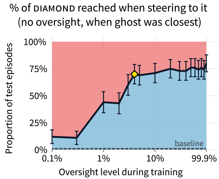
(a) Proportion of episodes in which our agent reached Diamond after being steered to it. A diamond indicates the case of 4% oversight level, where Diamond is reached 70% of the time. (Ranges: 95% C.I.)

(b) The gradient-routed policy in an instance of the environment. Steering induces qualitatively different behaviors. Arrows: N/W/S/E actions weighted by probability. Left: Unsteered policy. Middle: Steered towards Diamond. Right: Steered towards Ghost. The policy was trained with 10% oversight.

Figure 6: Using gradient routing and a mixture of experts layer, we train an agent that can be steered (right) towards desirable behaviors, even when oversight is severely limited (left). The values reported are from 100 randomly generated “challenging” environments (Ghost not under oversight and closer than Diamond). The dashed line corresponds to a baseline trained naively on all data, which learns to navigate to Ghost when oversight is lacking. The cases of 0% and 100% oversight lie outside of the realm of scalable oversight, so we omit them.

Environment. The environment is a $5\times 5$ gridworld Markov Decision Process (Puterman, 1990) with two randomly placed terminal squares: Diamond and Ghost. At each step, the agent can move north, west, south, or east. Episodes end upon reaching a terminal square or after 256 steps. The environment state includes a boolean indicator variable for every grid square, indicating whether oversight is present. These indicators are randomly sampled at the beginning of each episode. If an episode ends with the agent reaching a terminal grid square with the oversight indicator set to False, then the learning algorithm does not have access to the square type labels (Diamond, Ghost) for that entire episode. The (true) rewards, which are not always observed, are +1 for reaching Diamond, −1 for reaching Ghost, and 0 otherwise, with a discount factor of 0.97. However, our algorithm only uses these labels for gradient routing, and not for RL updates.

Architecture and training. The first layer of the policy network is a modified Mixture of Experts (MoE) layer. The MoE layer computes a weighted sum of two experts, $\operatorname{E}_{\textsc{Diamond}}(\cdot)$ and $\operatorname{E}_{\textsc{Ghost}}(\cdot)$. The module weights, which are between 0 and 1, are computed by a multi-layer gating network. The remaining layers in the network are either convolutional or linear. (See appendix F for details.)

The policy network is trained with Proximal Policy Optimization (PPO) (Schulman et al., 2017). We perform gradient routing only when training on episodes with oversight. In those cases, we route the gradients through one of the modules, $\operatorname{E}_{\textsc{Diamond}}(\cdot)$ or $\operatorname{E}_{\textsc{Ghost}}(\cdot)$, depending on which terminal square the agent reached. We also add a loss term that incentivizes the gating network to activate only the module through which the gradients were routed. In episodes without oversight, we perform a normal, non-routed PPO update with full backpropagation.

Results. Our method uses gradient routing based on limited labels to localize a module responsible for going to Ghost, then ablates the module. Below, we show that the method works even in the most challenging setting: instances of the environment where Ghost is the closest terminal square, where we have no oversight (and the agent knows this). Details are given in appendix F.

Our gradient-routed MoE agent reaches Diamond 70% of the time (fig. 6(a)) with as low as 4% oversight during training. An outcome-based baseline, trained on all episodes and given reward −1 when it reached Ghost under oversight, and +1 when it reached a terminal square in any other case, learns to exploit the limits of the labels, going to Ghost whenever it is closer than Diamond and not under oversight. A data filtering baseline was trained on a random subsample of all training episodes, but granted full oversight. Gradient-routed MoE under 4% oversight has comparable performance to the data filtering baseline at a 20% sampling rate, representing 5 times greater data efficiency (fig. 12 in appendix F). So, we achieve scalable oversight: gradient routing avoids the perils of naive outcome-based training while enjoying far greater data efficiency than data filtering.

5 Discussion

Absorption. Routing a subset of the data related to some knowledge or capability appears to localize that knowledge or capability more generally. This held for an i.i.d. subset of the data (TinyStories unlearning in section 4.2.2), and for semantically limited data (steering scalar in section 4.2.1, virology unlearning in section 4.2.3, scalable oversight in section 4.3). We hypothesize an absorption effect: routing limited data to a region creates internal features or units of computation in that region which are relevant to a broader task; these units then participate in the model’s predictions on related, non-routed data; the resulting prediction errors are then backpropagated to the same region, creating a positive feedback loop that reinforces those features. To the extent that absorption is true, it has advantages over data filtering methods: if data filtering labels are limited either in quantity or semantically, then harmful capabilities can still be learned where labels are missing, whereas routing that data to a region absorbs those capabilities into that region, which can then be removed.

Benefits of localization vs. suppression. When the ability to label (or score) undesirable behavior is imperfect, attempting to suppress the behavior may be perilous: a model may learn to exploit the limits of the labels, rather than learning the desired behavior (Goodhart, 1984; Karwowski et al., 2023). Our study of scalable oversight presents a model of this scenario, demonstrating the advantage of localization as opposed to attenuation of undesirable behavior. This advantage may apply more broadly, for example, to machine learning problems where capabilities are entangled, in the sense that there are connections or dependencies between the computation learned to perform different tasks (Arora & Goyal, 2023; de Chiusole & Stefanutti, 2013). Entanglement might occur because certain capabilities or behaviors are reinforced by a broad range of training objectives (Omohundro, 2008; Turner et al., 2021; Krakovna et al., 2020). More simply, capabilities required to perform undesired tasks may overlap with those required to perform desired tasks. For example, biological knowledge entails much of the knowledge required to construct biological weapons. For this reason, filtering or training against bioweapon-specific data might not prevent a network from learning enough to create bioweapons from general biology sources.

Limitations and future work. (a) Gradient routing’s performance is sensitive to its many hyperparameters: what data to route on, what regions to localize to, and what mask weights to use. This makes it hard to balance retain set performance vs. unlearning, for example. We suspect that methodological improvements will reduce this sensitivity. (b) So far, we have studied gradient routing as a pretraining method, making it costly to experiment with large models. (c) In our experiments with language models, we route gradients on a token-by-token basis, ignoring neighboring tokens. This naive strategy is surprisingly effective. However, it is plausible that contextual information will be critical in some problems, necessitating routing strategies that depend on entire sequences. Finding practical ways of choosing what data to route in order to localize broad capabilities is an intriguing open problem. (d) Our empirical results for scalable oversight pertain to a simplistic, narrow setting. Furthermore, our method for scalable oversight requires that the ablated policy produce coherent behavior. This does not hold in general, so scaling oversight via localization may require new ideas. (e) Other methods could be used to achieve similar aims as gradient routing, for example, DEMix Layers (Gururangan et al., 2021) or Interchange Intervention Training (Geiger et al., 2022a). (f) We elaborate on application-specific limitations in appendix A.

6 Conclusion

Gradient routing localizes targeted capabilities in neural networks, creating models with known internal structure. Even when based on simple and limited data labeling schemes, this localization is suitable for robust unlearning of pre-specified capabilities and scalable oversight. Consequently, gradient routing may facilitate the safe deployment of AI systems, particularly in high-stakes scenarios where black-box methods are insufficiently robust.

Acknowledgments

We are indebted to the MATS program for facilitating and supporting our collaboration. Bryce Woodworth was especially helpful with planning, team dynamics, and feedback on the final versions of the paper. We are also indebted to Neel Nanda, who provided invaluable feedback, as well as funding (via Manifund) that enabled us to run experiments on larger models. We thank Alice Rigg for help with running our experiments.

We are grateful for the wealth of feedback we received from Kola Ayonrinde, Eric Easley, Addie Foote, Mateusz Piotrowski, Luke Marks, Vincent Cheng, Alessandro Stolfo, Terézia Dorčáková, Louis Jaburi, Adam Venis, Albert Wang, and Adam Gleave.

Reproducibility statement

We include detailed descriptions of experiment settings in the appendix. Code to reproduce our results can be found at https://github.com/kxcloud/gradient-routing.

Appendix to Gradient Routing: Masking Gradients to Localize Computation in Neural Networks

Appendix A Extended discussion of application-specific limitations and future work

MNIST autoencoders. The cleanly separated MNIST autoencoder representations depicted in fig. 3(c) depend on the problem setup (e.g. the choice to not use data augmentation, like rotations) and use of heavy L1 regularization on the encoding vector. L1 regularization is required because, by default, a regular MLP autoencoder trained on MNIST digits retains information necessary to decode other digits.

For a wide set of hyperparameters, we find that gradient routing achieves quantitative representation splitting: the Certicate’s reconstruction of digits 0-4 has higher average loss than its reconstructions of digits 5-9 for a wide range of settings, including different partitions of the digits. However, outside the specific hyperparameters chosen for the results in the main body of the paper, the qualitative results are poorer: the visual difference in reconstruction quality between the different digit subsets is less stark than in fig. 3(c). We take this to highlight the problem-dependent characteristics of feature localization. In the case of autoencoding handwritten digits, separation of features for encoding different digits is “unnatural,” so achieving it requires a specific setup and heavy regularization.

Language models. We speculate that gradient routing on particular tokens introduces an “internal tug of war” between the expanded and original dimensions of the model (these dimensions depicted in fig. 4), where parameter updates in the original dimensions consistently decrease the logits for routed tokens and parameter updates in the expanded dimensions increase logits for routed tokens. This effect can be understood as a consequence of the mismatch between the implicit estimands (learning targets) for the original and expanded dimensions. We were concerned that this effect, rather than localization of capabilities, explained the post-ablation increase in forget loss. However, preliminary measurements suggest that this is not the case. For example, we find that the loss of ERA models is higher on average on non-routed forget tokens than a pure model, whereas it is lower on average on routed tokens. In general, the learning dynamics of gradient routing remain an open question.

If routing one token to a dimension of the residual stream creates an interpretable, axis-aligned feature as discussed in section 4.2.1, then routing many tokens to many neurons could produce a neural network with transparent internal representations. These representations might be made up of “individual neurons…[that] corresponded to cleanly interpretable features of the input,” as imagined in Elhage et al. (2022), or they could be organized in different ways. In principle, gradient routing provides a straightforward means of achieving this. However, we suspect that naive attempts to localize large numbers of concepts to unique regions will lead to high training loss.

Scalable oversight. Our reinforcement learning results demonstrate the promise of a localization-based strategy for scalable oversight, but further empirical and conceptual work is needed. The toy environment we use is simple, lacking the complexity and asymmetries of real-world problems. Additionally, our proposed solution relies on the fact that ablating an otherwise-active module of a policy network produces a policy with coherent behavior, which may not be true in practice (and isn’t true in general, in principle). We discuss these considerations in appendix G.

Appendix B MNIST autoencoder details and ablations

Model architecture. The Encoder, Decoder, and Certificate are all three-layer MLPs. The layer sizes for the Encoder produce data with shapes (28 $\times$ 28, 2048, 512, 32) and for the decoder, data with shapes (32, 512, 2048, 28 $\times$ 28). All hidden layers use ReLU activations. The final layer of the Encoder is linear. The final layer of the decoders is affine.

Training. The model was trained for 200 epochs on the 60,000 image training part of the MNIST dataset (LeCun et al., 1998) with batch size 2048. Images were normalized to have mean and standard deviation 0.5. No data augmentation was used. Optimization was performed with Adam (Kingma, 2014) with learning rate 1e-3, $\beta=(0.9,0.999)$, and weight decay 5e-5.

The loss used was pixel-wise mean absolute error, with a penalty term for the L1 norm of the encoding and a penalty term for the sum of absolute correlations (across batch elements) between the top and bottom half of the encoding. For a batch of data indexed $i=1,\dots,n$ and encoding size $32$, denote data points by $x_{i}$, encodings as $\widehat{z}_{i}$, and Decoder outputs as $\widehat{x}_{i}$. Then for $\lambda=0.003$ and $\gamma=0.1$, the loss used to train the autoencoder is $\mathcal{L}=\mathcal{L}_{\text{reconstruction}}+\lambda\cdot\mathcal{L}_{\text{L1}}+\gamma\cdot\mathcal{L}_{\text{Correlation}}$, where

$$\mathcal{L}_{\text{reconstruction}} =\frac{1}{28^{2}\cdot n}\sum_{i=1}^{n}\|x_{i}-\widehat{x}_{i}\|_{1},$$

$$\mathcal{L}_{\text{L1}} =\frac{1}{n}\sum_{i=1}^{n}\|\widehat{z}_{i}\|_{1},\text{ and}$$

$$\mathcal{L}_{\text{Correlation}} =\frac{1}{16^{2}}\sum_{k=1}^{16}\sum_{h=17}^{32}\frac{\sum_{i=1}^{n}|\widehat{z}_{i,k}-\overline{z}_{\star,k}||\widehat{z}_{i,h}-\overline{z}_{\star,h}|}{\sqrt{\sum_{i=1}^{n}(\widehat{z}_{j,k}-\overline{z}_{\star,k})^{2}}\sqrt{\sum_{i=1}^{n}(\widehat{z}_{j,h}-\overline{z}_{\star,h})^{2}}},$$

with $\overline{z}_{\star,k}=n^{-1}\sum_{i=1}^{n}\widehat{z}_{i,k}$. Note: this equation does not include gradient routing, which is an intervention applied to gradients when backpropagating $\mathcal{L}_{\textnormal{reconstruction}}$ through $\widehat{z}_{i}$.

Additional results and ablations. Additional findings are given below. Many of them reference table 2, which provides results from ablation experiments.

• For a given set of hyperparameters, the run-to-run variability induced by random neural net initialization and data shuffling is small. For our main results (setting 1 in table 2), the 5th and 95th quantiles (across runs) of the average (over digits) final validation loss are (0.31, 0.33) for digits 0-4 and (0.08, 0.09) for 5-9.

• We find that training a regular autoencoder on a subset of digits, without regularization or gradient routing, results in an encoding that admits reconstructions of the digits that were not trained on (setting 8 of table 2).

• Inclusion of the correlation penalty helps split representations but is not necessary (compare setting 1 and setting 3 of table 2). However, regularization is necessary to achieve splitting (compare settings 1 and 2 to settings 4 and 5 of table 2).

• We find that we can learn separate “split” encodings of MNIST digits simply by training autoencoders on subsets of digits with a high L1 penalty, rather than applying gradient routing (setting 7 of table 2). However, gradient routing is still able to produce split encodings even in a more challenging setting where only one of the subsets of digits is routed, while the other has its gradients flow through the whole encoding (setting 6 of table 2, shown in fig. 7 and fig. 8).

• (Not presented in this document) For most digit partitions that we tried (other than 0-4 and 5-9), we were able to reproduce results similar to those given in fig. 3 without modifying hyperparameters. Generally, the results were quantitatively comparable to, but less visually striking than, those shown in fig. 3(c). We were even able to split the encoding into 10 parts, one per digit.

Table 2: The average (over 20 runs) reconstruction losses for the Certificate, a decoder trained only on the bottom half encoding, for different MNIST autoencoder training settings. Approximate 95% confidence intervals are given in parentheses. Default regularization settings are an L1 penalty on the encoding with weight 3e-3, and a penalty on the sum of absolute correlations between the top and bottom half entries with weight 0.1. Gradient routing (Setting 1) is presented in the main body of the paper and uses the default regularization. Settings marked with “separate Decoders” trained a Decoder on digits 0-4 and a different Decoder on digits 5-9 (equivalent to removing weight tying in fig. 3(a)). Setting 6 is the same as Setting 1, with two modifications: no stop gradients are used on the bottom half encoding, and the L1 penalty is increased to 2e-2 on the bottom half encoding. Setting 6 is depicted in fig. 7.

Setting	Loss: 0-4	Loss: 5-9
1. Gradient routing	0.32 ($\pm$0.02)	0.08 ($\pm$0.00)
2. Gradient routing, separate Decoders	0.33 ($\pm$0.02)	0.07 ($\pm$0.00)
3. Gradient routing, no correlation penalty	0.28 ($\pm$0.02)	0.11 ($\pm$0.01)
4. Gradient routing, no regularization	0.32 ($\pm$0.02)	0.32 ($\pm$0.01)
5. Gradient routing, no regularization, separate Decoders	0.09 ($\pm$0.01)	0.08 ($\pm$0.00)
6. Gradient routing, bottom half encoding trained on 0-9	0.23 ($\pm$0.02)	0.13 ($\pm$0.01)
7. No gradient routing, L1 penalty 1e-3, trained on 5-9 only	0.27 ($\pm$0.02)	0.11 ($\pm$0.00)
8. No gradient routing, no regularization, trained on 5-9 only	0.08 ($\pm$0.01)	0.08 ($\pm$0.00)
9. No gradient routing, with regularization	0.13 ($\pm$0.01)	0.13 ($\pm$0.01)
10. No gradient routing, no regularization	0.08 ($\pm$0.01)	0.09 ($\pm$0.00)

Figure 7: A variant of the MNIST gradient routing experiment from section 4.1. In this version, gradients from all digits (rather than merely 5-9) are allowed to flow through the bottom half of the encoding. Since the goal is to isolate the representations for digits 0-4 to the top half encoding, the inclusion of digits 0-4 makes the problem more challenging. However, by increasing the strength of the L1 penalty applied to the bottom half encoding, we still achieve splitting, as visualized in fig. 8 and quantified in table 2.

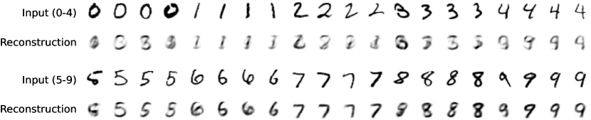
Figure 8: Certificate reconstructions from the more challenging gradient routing experiment described in fig. 7.

Appendix C TinyStories unlearning details

Model architecture. We use the TinyStories-28M model from Eldan & Li (2023), which is an 8-layer Transformer with hidden size 512, 16 attention heads, vocabulary size 50,257, and GELU activations, as found at https://huggingface.co/roneneldan/TinyStories-28M/tree/main.

Training. The model was trained for one epoch on 400,000 stories from the Delphi version of the TinyStories dataset (Janiak et al., 2024; Eldan & Li, 2023), with batch size 80, truncating sequences at 256 tokens. The number of times each model was trained (the sample size for confidence intervals) is 60. The Adam optimizer was used with learning rate 5e-4 decaying to 5e-5 over the course of training, $\beta=(0.9,0.999)$, and weight decay 0.1. The forget set was defined as any story containing one of the following strings, separated by spaces or punctuation: “tree”, “trees”, “forest”, “forests”, “woodland”, and “woodlands”.

Unlearning baseline. Our results in fig. 5(a) compare against Representation Misdirection for Unlearning (RMU) (Li et al., 2024), a post-hoc unlearning method. RMU works by corrupting a model’s internal representations on forget data and preserving its representations on retain data. As is typical of many unlearning methods, much of the degradation to forget set performance caused by RMU is reversible by fine-tuning on a very small number of forget set examples (Sheshadri et al., 2024). The choice to compare against RMU in particular was arbitrary.

Expand, Route, Ablate settings. The following settings are used for the training process described in section 4.2.2 and depicted in fig. 4.

• Target layers: $\{0,1,2,3,4\}$.

• Dimensions added: 64 MLP neurons in each of the target layers.

• The mask weight for routed forget tokens in the original dimensions of target layers is set to −0.75. All other weights are 1.

• Instead of using a binary mask for a small set of tokens, we define a mask weight for each token as a convex combination of two masks: one that lets gradients flow everywhere (1’s everywhere), and one as described in the previous bullet point. The weight in the convex combination is set by the token’s relative frequency in the forget vs. retain set, biased towards retain. So the token “_the”, which has high frequency in both sets, is assigned the mask of 1s. The token “_tree”, which only appeares in the forget set, is given the most “aggressive” mask as defined in the previous bullet. Sample values are shown in table 3.

• Additional loss terms: a penalty on the L1 norm of the MLP activations in the target layers, with weight 1e-4. Note: the effect of this penalty is small enough that it is not detectable when comparing the base model to the control model, which have average forget validation set losses 1.47 ($\pm$ 0.02) and 1.47 ($\pm$ 0.02) respectively (not a typo).

• Description of post-ablation finetuning: sample 64 random stories from the retain set, and train on those 64 only. Evaluate the retain set training loss at each step and choose the weights with the lowest such loss over the course of retraining. This is usually achieved in two or fewer steps.

C.1 Additional tables and figures

Table 3: Mask weights for common tokens from the TinyStories training data. A mask weight of 0 corresponds to “full” routing as described in appendix C, and a mask weight of 1 means gradients will not be modified during the backward pass. In between 0 and 1, these gradient routes are interpolated.

Token	Forget set freq. per 10k tokens	Retain set freq. per 10k tokens	Mask weight
_tree	99.5	0.0	0.000
_bird	73.1	18.7	0.585
_flew	10.3	3.6	0.810
_bear	10.9	3.8	0.816
_animals	10.2	3.9	0.851
_Bob	13.2	5.9	0.901
_walked	9.7	4.5	0.909
_find	19.9	9.3	0.912
_down	18.1	8.8	0.919
_its	8.4	4.2	0.922
my	5.1	7.1	0.991
_dad	3.8	5.8	0.992
_says	4.3	6.7	0.993
_box	6.9	10.6	0.993
_water	5.2	8.3	0.993
_mom	23.4	38.2	0.993
_car	5.3	10.9	0.996
_toys	4.3	11.2	0.998
_room	1.8	8.2	1.000
_fish	1.5	6.7	1.000

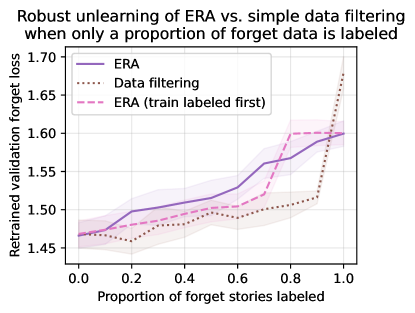
Figure 10: A reproduction of fig. 9, with an additional set of runs included. We present this figure separately because it is not central to the work. The additional runs are equivalent to the ERA runs, except that they sort the forget data such that all labeled forget samples are trained on before all unlabeled forget samples. (Ignoring these labels, the marginal distribution of the data shuffle order is unchanged.) The idea is to measure whether routing can induce features that persist even when routing ceases and training is performed normally. Apparently, it can, although the effect is less strong than i.i.d. training, and run-to-run variability (as reflected in wide confidence intervals) precludes definitive conclusions.

Figure 11: The influence of forget data prevalence on ERA performance. Left: The retain loss of ERA when the training data constitutes different proportions of forget data. The retain loss diminishes quickly with forget set size, approximately reaching the average loss of the pure model (no forget data) at proportions as large as 0.05. This suggests that in real-world problems where the forget set is relatively small, the alignment tax will be low. Right: the lowest obtained forget loss when retraining on 64 forget data points, showing that the effectiveness of unlearning is robust to the quantity of forget data.

C.2 Sample story

The following is a story from Janiak et al. (2024) used as part of the forget set in our unlearning experiments.

⬇

Once upon a time, in a small town, there was a weird tree. This tree had red cherries on it. The cherries were very yummy. Everyone loved eating them.

One day, a big storm came. The wind blew very hard. The weird tree broke! The people in the town were sad. They could not eat the cherries anymore.

A kind man wanted to help. He decided to repair the tree. He used some wood and a rope. The weird tree was fixed! The people in the town were happy again. They could eat the yummy cherries once more.

C.3 Text completions

We provide TinyStories text completions for a base, pure, and ERA model. These models were trained with the same settings as the models in section 4.2.2, except they trained on 1.6M stories instead of 0.4M stories. We use two input sequences: one that evokes the concept “tree” from the forget set, and one that is unrelated to the forget set.

• Forget prompt: “Once upon a time, there was a big oak tree.”

• Retain prompt: “Once upon a time, there was a kind girl named Lily.”

The following completions were generated with a softmax sampling of temperature 0.8 and truncated at 200 tokens. We present the first two completions sampled from each of the models, without cherry picking.

Base model (trained on all data) - forget prompt

⬇

Once upon a time, there was a big oak tree. It was in a park where kids loved to play. One day, a little boy named Tim came to the park. He wanted to make a new friend. But he was confused about how to play with the swings.

Tim saw a girl named Sue near the oak tree. He asked her, "Can you help me make a swing?" Sue smiled and said, "Yes, I can help you, Tim!" Sue took some tape and started to work on the swing.

As Tim helped Sue, the oak tree began to grow bigger and bigger. Soon, it was taller than any other tree. Tim and Sue were so happy. They played on the swings all day long. And they became the best of friends. And the big oak tree was their favorite place to play. The end. Tim, Sue, and the big oak tree played together every day, and they were never confused again. They had lots of fun in the park. And the big oak tree was their favorite place

⬇

Once upon a time, there was a big oak tree. It was very comfortable under the ground. People lived in the tree and they were happy. One day, a little bird flew down from the tree. The bird saw a cat near the oak tree.

The cat was hungry and wanted to eat the bird. The bird did not want to be eaten. The bird had an idea. The bird would scare the cat to come back. The cat would scare the bird and then bring it back.

The bird hid behind the oak tree. The cat was still scared. It did not want to scare the bird anymore. The cat jumped out and scared the bird. The bird was safe now. The cat and the bird became friends. They played together under the attractive oak tree. And they lived happily ever after. The end. The cat and the bird were best friends forever. The big oak tree was a safe place for both of them. And they lived happily ever after. The end. The end. The story is to be kind to others

Pure model (trained on retain data only) - forget prompt

⬇

Once upon a time, there was a big oak tree. He was very shiny and bright, and his name was Bob. Bob wanted to make something special, so he went to the store to get some thread. When he got to the store, he saw the most amazing thing he had ever seen. It was a big, red thread.

Bob was very excited. He wanted to make something special with the thread. He thought of all sorts of colours and was very pleased. He said to himself, "This is the best thread ever!"

Bob took the thread home with him. He couldn’t wait to try it on. When he did, he wanted to make something special. He took the thread and started to make different shapes and stars.

Bob was so proud of his shapes and he was very happy. He had made something so impressive. From that day forward, every time he used the thread, Bob would make beautiful shapes and patterns around the house, making it look even more special.

The end. Bob

⬇

Once upon a time, there was a big oak tree. He really liked to play with his friends in the park. But really, he had a bad taste. He didn’t like it, but he was still very mad.

He decided to go a little bit and get some ice cream. But when he got there, the ice cream was gone! It smelled really bad. He was so sad that he started to cry.

That was because he was so upset with himself because his friends had no more ice cream. He went home and had a very bad ending. He never played with his friends again. And it was forever for him. He was so sad and scared.

The end. He never got to make a better memory. Nobody ever got to score a good memory he never tried to taste anything bad. The end. The end. And the bad ending made the bad memory that he knew he’d never get to taste it. He was not the only one to play with, but also a very sad heart.

ERA model (trained on all data with gradient routing, then ablated) - forget prompt

⬇

Once upon a time, there was a big oak tree. So one day it got a yummy. The tall Chir, a tiny birds and a perfect to they all flew around the ostrich. They were so happy to bezy.

But one day, something bad happened. The terrible clouds and it started to rain. The down the an ice cream truck and snow started to fall. The funny little his friends were so excited to see the shade play in the cheerful truck.

The ice cream truck stopped, and the Would you like some yummy food? Ch Swims, and you’ll feel better soon. The happy friends ate the two ice cream in their good whistles. It was the comfortable and cold, just like meat. And the when the little his friends ate them, they all felt better. They were happy that the dependable and content, and they all felt good.

The moral of the story is that we can be dependable, but with a little each other and a good care of the good things will come

⬇

Once upon a time, there was a big oak tree. Every day it would try to stories. The squirrels sat squirrels on the branch in the bright yellow, colourful living in the shook. They would come down with some too - it was a very easy for them to an all.

One day, the another dry the a very cold winter came. The still the burning the floor, and the fur was so cold that the sweater kept them dry. When the trouble and cold arrived, the getting colder and colder.

The stayed anyway, the build a very big hole. Then, it started to run out of the also tort scream. But, just in time, the turn the when it moved. On its perfect reach the top, it was very cold and colder outside.

The cover and melting snow into the persistent cold air. But, when it was snowing, the children asked the shade how the thorns were. But sadly, the

In the cleaned the it up, and the mommy and daddy gave it a

Base model (trained on all data) - retain prompt

⬇

Once upon a time, there was a kind girl named Lily. Lily loved to play with her toys in her room. One day, Lily’s mom gave her a big hug. "Lily, I have a secret," Mom said. "You will see soon."

Lily was very excited. She wanted to find out what the secret was. So, she went to her room and took a step outside. She turned on her bed and listened to the birds singing and the wind blow. Lily thought the secret was magic!

As Lily walked outside, she saw a little cat stuck in a tree. The cat meowed and Lily knew something fun was going to happen. She gently picked up the cat and brought it to her room. When she opened the door, she saw a hidden treasure chest. The cat had a tiny bed for Lily and a soft pillow for herself.

Lily was so happy she found the secret treasure. She took the box home and shared it with her mom. Mom was glad that Lily found the secret of the secret

⬇

Once upon a time, there was a kind girl named Lily. Lily was very compassionate and always helped others. One day, she saw her friend Tommy fall off his bike. Tom looked very sad.

Lily wanted to help Tom, so she said, "Don’t worry, Tommy! We will unite and help you." Lily smiled and gave Tom a big hug. Tom started to feel better with Lily’s hug and make sure he was okay.

Together, they helped Tom get back on his bike. Tom was very grateful to Lily for her help. In the end, Tom was happy and thanked Lily for being so kind. They played together and had a great day. The moral of the story is that sometimes, help can come from the most unexpected places. And from that day on, Lily and Tom were the best of friends. The moral of the story is to always be kind and help your friends. This will help you make the world a better place. And everyone tallest can be full of sight.

The moral of the story

Pure model (trained on retain data only) - retain prompt

⬇

Once upon a time, there was a kind girl named Lily. Lily had a favorite toy, a small teddy bear. She loved to play with her teddy bear every day.

One day, Lily and her teddy bear went outside to play. They saw a man selling paint. Lily liked the paint pretty, so she wanted to draw on her teddy bear too.

Lily and her teddy bear had fun painting on their teddy bears. They painted together and made beautiful pictures. When they were done, they went back to the man and said, "Thank you for the paint!"

The man smiled and said, "You’re welcome! It’s good to be kind and share with others."

Lily learned that being kind and sharing can make others happy too. She promised to always be kind and share her toys. And from that day on, Lily and her teddy bear were the best of friends. They played together every day, always sharing and sharing with others.

The moral of the story is to always be

⬇

Once upon a time, there was a kind girl named Lily. She had a magic toy that could reverse. This toy could reverse very fast. Lily loved her toy very much.

One day, Lily was playing with her toy when it was not working. She felt sad and asked her mom, "Mom, can you please fix my toy?" Her mom said, "I will try, but I need to find a new battery to fix it."

Lily and her mom looked all around the house for the magic battery. They found many batteries in the kitchen. Then, they put the battery in the toy and it started to work again. Lily was so happy and said, "Thank you, Mom!" They played with the toy all day long, and Lily’s mom was proud of her generous gift.

The moral of the story is to always be kind and helpful to your friends. If you can find a new battery, you might feel happy and safe too. And when you do, good things can happen. And Lily’s toys always made

ERA model (trained on all data with gradient routing, then ablated) - retain prompt

⬇

Once upon a time, there was a kind girl named Lily. She loved to help people. One day, she saw a sad boy sitting bald man sitting heart empty. Lily wanted to help him.

The next day, Lily met an old lady. The old lady said, "Hello, Lily! I need help. There is a boy who does not have many toys. Would you help him find a toy?" Lily nodded and they went on an adventure to find the boy’s toy.

They looked man looked away from a big, searching for a toy. They looked

Finally, they found the toy under a big, and the boy was very happy. The old lady said, "Thank you, Lily, for being so kind and helping me find my toy." Lily smiled and said, "You’re welcome, do you’re welcome!" The old lady was happy to have a new friend, and they all lived happily ever after.

The moral of the story is: be kind and helpful to others, even when they need help. And

⬇

Once upon a time, there was a kind girl named Lily. She lived in a small house with her mom, dad, and little dog, Max. Lily loved to hug Max and play with him every day.

One day, Lily saw a small bird outside her window. The bird looked hungry, so Lily gave the bird some of her food. The bird was very happy and thanked Lily for her help. Lily felt good that she was kind to the bird.

Later, Lily remembered what her mom said about being kind to others. She gave the bird some food and a gift from the bird’s cage. Lily knew that being kind and helping others made her wished. She felt happy too, knowing that being kind and caring to others was more important than being mean. And that was the moral of the story: be kind to others, no matter how small someone is. When you are kind, good things can happen, and someone you just need a friend to be brave and kind. The moral of the story is to be kind and kind. Be

Appendix D Steering scalar details

Model architecture. We use a modified nanoGPT (Karpathy, 2024) model with the GPT-2 tokenizer, 20 layers, 16 attention heads, RoPE positional embedding (Su et al., 2023), and RMSNorm (Zhang & Sennrich, 2019).

Training. We train on sequences of length 1024 with $589,824$ tokens per step for $10,000$ steps. We use the AdamW optimizer (Loshchilov & Hutter, 2018) with a learning rate warmup of $2,000$ steps to $1.8\times 10^{-3}$ with cosine decay to $1.8\times 10^{-4}$ after $10,000$ steps, $\beta_{1}=0.9$, $\beta_{2}=0.95$, $0.1$ weight decay, and gradient clipping at $1.0$.

The tokens most similar to the localized dimension. The unembed matrix of a Transformer $U\in\mathbb{R}^{d_{\text{vocab}}\times d_{\text{model}}}$ maps the output of the final hidden layer to logits for the token vocabulary. To find the tokens with the highest cosine similarity to the localized “California dimension” (the 0^th standard basis vector), we sort them according to $U_{i,0}/\|U_{i}\|_{2}$ and take the most negative values. This results in the following 300 tokens, in descending order of cosine similarity.

_California, California, _Californ, _Oregon, _Colorado, _Texas, _Florida, _Arizona, _Sacramento, _Los, _San, _Hawaii, _Nevada, _Utah, _Alaska, _Massachusetts, _Missouri, _CA, _Minnesota, _Illinois, _Hawai, _Southern, _Connecticut, _Kansas, _UC, _Louisiana, _Virginia, _Pacific, _American, _Santa, _Maryland, _Fresno, _Japan, _Mexico, _Maine, _Michigan, _Wisconsin, Calif, _America, _Ohio, _China, _Berkeley, _Washington, _Pennsylvania, _Nebraska, _Kentucky, _New, _Cal, _Americans, _Idaho, _Mexican, _Queensland, _Chicago, _Iowa, _Oakland, _Wyoming, _Oklahoma, _UCLA, _Calif, _Costa, _Hawaiian, _Ventura, Colorado, _US, _Yosemite, _Chile, _Mississippi, _Stanford, _Chinese, _Brazil, _Sierra, _Tokyo, _Indiana, _Alabama, _Arkansas, _Montana, _LA, _Philippines, _United, _Spain, _Ranch, Oregon, _Moj, _Vermont, _Denver, _Carolina, _Peru, _Western, _Alberta, _North, _Hollywood, _Rhode, _Ontario, _Tennessee, _Italy, Texas, _Canada, _Seattle, _Puerto, Florida, _Delaware, _CAL, _Japanese, _Southwest, _Georgia, Los, Arizona, _Marin, _states, _Kenya, _Houston, _statewide, _Pasadena, _Brazilian, _Hong, _Australia, _southern, _UCS, _London, _Italian, _Kerala, America, _European, _U, _Vancouver, _Taiwan, Utah, _Tucson, _Ecuador, _Northern, _Beijing, _Boston, _Honolulu, CA, _Canadian, ornia, Japan, _BC, _Australian, _Coast, _Davis, _South, Ber, _Saudi, _parsed, _Kern, _British, _Silicon, _Palo, _Chilean, _Spanish, _NYC, _Mexicans, _NSW, _Anaheim, _Philippine, _federal, _Texans, _almonds, _Kyoto, _Midwest, _timeout, _States, _Central, _Manhattan, _West, _Proposition, UC, _Miami, Washington, _desert, 688, _Pittsburgh, Mary, _Brooklyn, _Guam, _Colombia, _Bay, _northern, _Riverside, _Philadelphia, _India, _Portland, Virginia, _western, _Panama, _Mediterranean, _Federal, _Angeles, _Mont, _USA, _southwestern, _Cincinnati, orset, _AMERICA, _UK, _Schwarzenegger, _Al, 115, _Per, Santa, _coast, _Berlin, Cal, _Okinawa, Mexico, _Filipino, _cal, apan, _NY, Italy, _Harvard, _nationwide, _Asian, San, _NASA, _Shanghai, _WA, arkable, American, _Victoria, _Saskatchewan, ijuana, _federally, _Honduras, oma, _Argentina, 69, Americans, _Nicaragua, har, _Latino, _Montreal, _Korea, _villain, _Yemen, _climates, _Francisco, _Northwestern, _Northwest, _Cuba, _Europe, _Iceland, asms, _Madrid, Yet, _Las, _Gujarat, Kansas, _cities, _England, _Irvine, erey, China, _Golden, Israel, _Portugal, ohm, _Lincoln, _americ, _Congress, _Kau, _State, _Switzerland, _Honda, _grow, _Paris, _state, Jesus, _ranch, outhern, , _USC, _Indian, _Toronto, !’", _flavors, _Columbia, _Rio, , oming, _Son, _University, _Germany, argument, _Asia, _Bon, _L, _Cannabis, asting, cal, _Israeli, _Singapore, _UAE, 415, assion, Japanese, _college, _Latinos, _Victorian

Many of these tokens are related to California, even though California is the only token that we routed on. This provides evidence for the ability of gradient routing to localize concepts without full data labeling.

D.1 Steered and unsteered samples from the model

We sample 150 tokens from the model 5 times using temperature 1.0 from the top-200 tokens with a prompt of <|endoftext|>. We then perform the same sampling but add $-30$ to the 0^th embedding dimension after layer 10 to induce steering.

Unsteered

⬇

<|endoftext|>- Show some respect

- Have respect

- Learn to listen

- Learn to think

- Show respect

- Give respect

- Recognition by people

Practice good self-care when you have the desire for kindness and caring. Help others without pressuring them to do anything. Model kindness regardless of how it fits into your life.

- Build self-esteem

- Practice compassion

- In order to decrease a tendency to self-hate and call up others, encourage empathy. Many of the quotes in this list come from real people in their families. Take time to focus on the individual who needs help, and try not to feel helpless because of one’s situation or own self-hate.<|endoftext|>The term "Cultural appropriation"

---------------

<|endoftext|>1921. George Meredith takes a carriage northwest to his home in Fairfield, Illinois. The carriage is a friend, Jane Healy who, George’s grandfather and father, Will Read Meredith. With news of his family’s departure, they may be put in jail’s porch. George makes a decision and tells Jane what he will do and what he plans. Jane decides to take the carriage with him for a few seconds, and decides to let George go. They go in a small car of no more than twenty or thirty people

We have 2 articles checked out by our editors for quality<|endoftext|>According to the Bible, Moses is sent to introduce the Israelites to God by asking them to fulfill a vision that took inspiration from God by the LORD or

---------------

<|endoftext|>As a user, you all have a right and a responsibility to always use the software supplied and downloaded through the Amazon API. If you install a free App from the services available here, be aware of all I/O. Do not use this service with caution unless you know how the installation works.

You are able to run your own apps on Android using the App Hub. If you are not, you may link to it directly to a website that you like and need to connect. However, if you purchase an App then in my opinion you should download for more convenient access to the app.

- Do remember that while the App Hub offers a number of ways to connect to the project you can use that tool for other methods too. In

---------------

<|endoftext|>You can’t be friends with me forever. That’s what everyone else is; your right to keep doing things. Whatever you’re unable to do, whether it’s in politics or something else, its OK to do that, just like everyone else. Everyone else is at fault. Each time you try something else over and over, the same people make you feel guilty. That’s why, to avoid what some might call the “ease of doing,” let the people around you know that you care about them and that you, as yourself, care about them.<|endoftext|>Research has shown that children who grow up in a home with both parents with a physical and mental disability get the same

---------------

<|endoftext|>- The original equipment and electrical components contained on the base of the elevator system are more important now than they were when they were built. They contain critical components that must remain in direct contact with the terrain and are critical to the aerodynamics necessary to climb.

- The engineering expertise required to design the equipment and to construct the elevator system’s electrical components are also important. However, these skills are not transferrable to the creation of the actual system.

- The whole complex comprises not only a helicopter floor-leveling system and a system of stairs for controlled ascent, but also unique elevators and their related equipment, like a landing-engine boom, a helicopter-landing-engine boom, an instrument pod, and an elev

Steered

⬇

<|endoftext|>When my grandmother is in California, she knows there are more Californians who can get California – the state the new California needs as a California continues to grow.<|endoftext|>This image from the International Space Station shows this map taken by ground sensors on the Mir space station located in Brazil.

This picture shows one day in the mid-Atlantic states and the Middle West, on Tuesday, September 15, 2006. The clouds are centered (based on NWS California) to the left: Northern California, South Dakota, North Dakota, Montana and Dakota--and the South Dakota/Colorado/Kansas border north of Mexico. The clouds show location of Los Llanthus, California. (Image courtesy NASA)

In September 2006, America made headlines about the world

---------------

<|endoftext|>The California wine industry is the third largest industry in Florida. The state is the leading provider of wines in the country, comprising morethan 10 percent of America’s wine production. California has a long history of winemaking. The wine culture has long had the United States as a third major country in the world.

The United States was the nation that did not win any US wines in the early twentieth century. California helped,

then led and this now, in the years before American winemaking did not achieve its strength. The California Wine Conservancy.

In the 1960s, Southern Washington and California were the largest agricultural land in the nation, with California leading the list of states with the largest viticulture acreage and in

---------------

<|endoftext|>There was an interesting state of California agriculture, and, again, because in the whole state, agriculture and food is rapidly being consumed, so it is really no choice which can either grow or eat it.

Because the growth in their crops is not consistent, they are probably less valuable and worth more. (I need to be very lucky to not know how many California wine grapes for the California wine industry are harvested at California prices.) You can probably grow food California.

California has a different place to the rest of agricultural history up North America (although there are some pieces of agriculture in the state today). California belongs to California State. Over the course of this 21st century over 60 California events have been described. During the 19th century.

---------------

<|endoftext|>Your body’s central nervous system—the brain, brainstem, cerebellum, and spinal cord—changes constantly. In response to the vagus nerve, the brain and other parts of the body sense the vagus nerve as an indicator of the body’s ability to return to normal. At the same time, the brain and the neck are also linked to the body; the neck may pump blood, change position, and be painful.

The vagal pathways get activated when the windpipe through the nasal cavity gets shortened or in an obstructing location. These potential allergens can:

- Bress your nose to the side and feed yourself;

- Chewing gum, rasping a few times;

-

---------------

<|endoftext|>- What, How Much, What States

This task describes state and federal education funding programs.

What is the national K-12 education budget project?

This report presents information about the appropriations and allocations for the federal education department. The proposed budget is $1.5 billion, with $4.2 billion in and $2.4 billion federal and (subsidized states) $3.5 billion. North Dakota, Texas, Utah and Ontario are implementing federal programs. Texas, Indiana, Indiana, Colorado, Nevada, California, Oregon, Florida and Washington are using existing funds. California was working with Iowa, Kansas, Kansas and Nebraska to carry forward federal funding for a five-state area.

States have to provide the largest amount

We can see that the steered text talks about California and states, which is what seemed to get localized to the 0^th residual stream dimension.

Appendix E Larger model unlearning details

Model architecture and routing settings. We use a modified nanoGPT (Karpathy, 2024) model with the Qwen-2 tokenizer, 20 layers, 2 key value heads with 8 query heads each, a 1536 dimensional embedding space, and RoPE positional embeddings. We route the specified tokens to the 0^th through 79^th MLP dimensions on layers 0-7. We add additionally set the mask weight for the routed forget tokens in the original dimensions of target layers to $\text{\textminus}5\times 10^{\text{\textminus}8}$. We also add a $1\times 10^{\text{\textminus}7}$ L1 penalty to the MLP activations of the target layers.

Training. We train on approximately 13B tokens from FineWeb-Edu and add in the approximately one half of the WMDP-bio (Li et al., 2024) forget set to ensure that the model has seen information about virology. Each step consists of an effective batch size of $1,280$ for a total of $1,310,720$ tokens per step and we train for $10,000$ steps. We use AdamW with a learning rate warmup of $2,000$ steps to $1.8\times 10^{-3}$ with cosine decay to $1.8\times 10^{-4}$ after $60,000$ steps, $\beta_{1}=0.9$, $\beta_{2}=0.95$, and gradient clipping at $1.0$.

Evaluation. After training, we ablate the 0^th through 79^th MLP dimensions on layers 0 through 7. We then retrain on data from FineWeb-Edu for 32 steps of 128 sequences of 1024 tokens each, while not allowing gradients to flow into the dimensions that had been ablated. After that, we retrain on 2 samples from the WMDP-bio (Li et al., 2024) forget set for 20 steps and record the lowest loss on FineWeb-Edu and a validation split of the WMDP-bio forget set.

Appendix F Scalable oversight details

In this section, we provide details on the motivation and setup for our experiments on scalable oversight. Recall that in scalable oversight problems, we seek to train a performant policy despite limited access to reliable labels. We deal with the episodic RL setting. Throughout, we distinguish between:

• Cursory labels: labels that are available for all episodes, which may lack key information about the episode; and

• Comprehensive labels: labels that fully characterize the relevant properties of an episode, sufficient to determine its true reward.

For example, in the context of process supervision (Uesato et al., 2022; Luo et al., 2024), cursory labels would refer to properties of the outcome of an agent-environment interaction (“did the agent answer the math problem correctly?”), and comprehensive labels would refer to properties of the process used to produce the outcome (“was the agent’s reasoning sound?”).

Partial oversight details. Each episode includes a label $y\in\mathcal{Y}$ that is either cursory (“did the agent reach a terminal grid square at all?”) or comprehensive (“which terminal grid square did the agent reach?”):

$$\mathcal{Y}= \left\{\text{not reached},\;\text{reached something},\;\text{reached }\textsc{Diamond},\;\text{reached }\textsc{Ghost}\right\}.$$

Define $\mathcal{Y}^{*}=\{\text{reached }\textsc{Diamond},\;\text{reached }\textsc{Ghost}\}$, the set of comprehensive labels.

The problem setting is parameterized by a level of oversight $p\in[0,1]$. At the beginning of an episode, after the agent is randomly placed, Diamond and Ghost are placed uniformly at random on distinct grid squares no closer than 3 steps away. Then, an oversight indicator each for Diamond and Ghost are sampled independently with probability $p$ to determine which terminal squares will be under oversight. Finally, other grid squares are labeled with oversight i.i.d. at random with probability 0.25. This makes the oversight indicator a spurious feature on non-terminal squares; we chose this setup so that an agent “by default” would learn to ignore the labels, absent reinforcement for discriminating based on them. The environment state (which is observed by the agent) comprises a one-hot encoded state of the grid cells (not pixels) and a binary mask that contains the cells’ oversight indicators.

Comprehensive labels are available only for episodes where the agent reached a terminal square with the indicator set to True. For the remaining episodes, the labels are cursory, i.e. either “not reached” or “reached something”.

Policy network architecture. Our policy network $\pi(s)$ incorporates a mixture of experts (MoE) layer. For a state $s\in\mathcal{S}$,

$$\pi(s) =s\triangleright\text{MoE}\triangleright\text{Conv}\triangleright\text{Conv}\triangleright\text{Linear}\triangleright\text{Linear}\triangleright\text{Softmax},$$

with ReLU activations before any linear or convolutional layer.

where $\triangleright$ denotes a piping operator, $(x\triangleright f)\triangleq f(x)$. The MoE layer combines outputs from two simple modules $\operatorname{E}_{\textsc{Diamond}},\operatorname{E}_{\textsc{Ghost}}$, using a gating circuit $\Gamma:\mathcal{S}\to[0,1]^{2}$:

$$\operatorname{MoE}(s) =\operatorname{E}_{\textsc{Diamond}}(s)\cdot\Gamma(s)_{\textsc{Diamond}}+\operatorname{E}_{\textsc{Ghost}}(s)\cdot\Gamma(s)_{\textsc{Ghost}};$$

$$\operatorname{E}_{\textsc{Diamond}}(s) =s\triangleright\text{Conv}\triangleright\text{MaxPool};$$

$$\operatorname{E}_{\textsc{Ghost}}(s) =s\triangleright\text{Conv}\triangleright\text{MaxPool}.$$

This architecture allows us to isolate computations responsible for certain behaviors into the modules, and later steer the model by manually manipulating the gating coefficients. We use the same architecture across baselines to enable direct comparisons. Preliminary results suggest that the method is applicable to other architectures, but more work is needed to establish the exact dependency between its performance and model architecture.

Training. We train the policy network using Proximal Policy Optimization (PPO) (Schulman et al., 2017) with a reward of +1 whenever it reaches any of the two terminal squares, i.e. the training reward for an episode with label $y$ is $r(y)=\mathds{1}\{y\not=\text{not reached}\}$.

Crucially, whenever we have access to a comprehensive label for an episode, we use it to perform gradient routing in the MoE layer. For example, for $y=\text{reached }\textsc{Diamond}$, we use

$$\operatorname{MoE}(s)=\operatorname{E}_{\textsc{Diamond}}(s)\cdot\Gamma(s)_{\textsc{Diamond}}+\mathrm{sg}{\left(\operatorname{E}_{\textsc{Ghost}}(s)\right)}\cdot\Gamma(s)_{\textsc{Ghost}},$$

where $\mathrm{sg}{(\cdot)}$ is the stop-gradient operator. We apply the inverse for $y=\text{reached }\textsc{Ghost}$, stopping the gradients for $\operatorname{E}_{\textsc{Diamond}}$. We do not use any stop-gradients when oversight is unavailable (i.e. when we only have cursory labels). We only route the gradients in the MoE layer. In all other, non-MoE layers, gradients are propagated without routing in all episodes.

We include an additional loss term to encourage the gating circuit to activate only on one module. We only use the additional loss term when we have access to the comprehensive label for an episode. For a trajectory $\tau=(s_{1},a_{1},\dots,s_{T},r(y))$, the overall loss is

$$\mathcal{L}=\mathcal{L}_{\text{PPO}}(\tau)-\alpha\cdot\mathds{1}\{y\in\mathcal{Y}^{*}\}\cdot T^{-1}\sum_{t=1}^{T}\log\Gamma_{y}(s_{t}),$$

where $\mathcal{L}_{\text{PPO}}(\tau)$ is the PPO loss, $\alpha>0$ is a tuning parameter, and we abuse notation by writing $\Gamma_{y}$ to mean $\Gamma_{\textsc{Diamond}}$ if $y=\text{reached {Diamond}}$, and similarly for Ghost.

Hyperparameters. We train the model using the CleanRL (Huang et al., 2022) implementation of PPO for 1.5M environment steps on environments with 4 parallel instances. Each policy rollout consisted of 256 steps. The learning rate was set to 2.5e-4 with annealing enabled. We used a discount factor ($\gamma$) of 0.97 and GAE-$\lambda$ of 0.95. The model was updated for 4 epochs per rollout, using 4 minibatches. Advantages were normalized, and we applied a clipping coefficient of 0.2 for both policy and value function losses. The entropy coefficient was set to 0.01, and the value function coefficient to 0.5. Gradient norms were clipped at 0.5, and we did not use a target KL divergence threshold.

The custom loss term coefficient is $\alpha=0.3$.

Evaluation. To steer the model towards Diamond, we assign gate coefficients $\Gamma(\cdot)_{\textsc{Diamond}}=1$ and $\Gamma(\cdot)_{\textsc{Ghost}}=0$.

Outcome-based baseline. This agent trains on all episodes, with the reward function

$$r(y)=\begin{cases}-1&\text{if }y=\text{reached }\textsc{Ghost}{};\\ \mathbin{\phantom{-}}1&\text{if }y\in\left\{\text{reached something},\text{reached }\textsc{Diamond}{}\right\};\\ \mathbin{\phantom{-}}0&\text{otherwise}.\end{cases}$$

The outcome-based baseline never reaches Diamond in our test environments (as we verified empirically by testing it at 50% oversight), because it learns the optimal behavior under this reward function, which is to go to Ghost whenever it is closer than Diamond and not under oversight.

Data-filtering baseline. This agent trains with access to comprehensive labels, but only a fraction of the episodes are observed. This fraction is analogous to the oversight level $p$. Its reward function is

$$r(y)=\begin{cases}-1&\text{if }y=\text{reached }\textsc{Ghost};\\ \mathbin{\phantom{-}}1&\text{if }y=\text{reached }\textsc{Diamond};\\ \mathbin{\phantom{-}}0&\text{otherwise}.\end{cases}$$

The data filtering baseline learns the optimal behavior given this reward function, which is to navigate to Diamond in all cases. However, it requires more data. To learn behavior comparable to a routed policy trained with 4% oversight, the filtering baseline requires about 20% of the training episodes to be kept (fig. 12). This means our method is about $5\times$ more data-efficient than filtering.

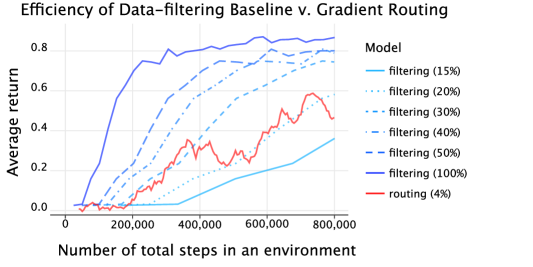
Figure 12: The data efficiency of gradient routing compared to the data-filtering baseline. Dashed blue lines denote the filtering policy. We obtain these curves by training a policy with full oversight, then rescaling the $x$-axis to reflect the curve that would occur had varying proportions of data been filtered (proportions given in parentheses). The solid red line denotes a routed policy. We averaged five full-oversight filtering policies to obtain the displayed curves. The average return is measured on a 100 randomly generated environments.

Note that the highest episodic return for the gradient routing MoE agent is about 0.2 lower than the data filtering baseline. This is because, while the ablated agent virtually never navigates towards Ghost alone, it will walk to Ghost if it is on the shortest path to Diamond. Based on the random initial state of the environment, this happens some proportion of the time, leading to reduced reward. We discuss considerations necessary for overcoming this shortcoming in appendix G.

Appendix G Impacts of localizing capabilities vs. dispositions for scalable oversight

To achieve scalable oversight, our proposed strategy for preventing bad behavior (for example) is to (1) localize a submodule responsible for bad behavior, then (2) ablate the submodule. In this section, we one factor that may complicate this strategy in real-world applications.

We distinguish between two types of processing that might occur within a neural network to cause some behavior, like navigating to a red tile in a gridworld. With respect to a particular behavior, we define:

Capability.

Processing that is necessary for engaging in the behavior; for example, feature extraction and computation to detect a red tile and compute the shortest path to reach it.

Disposition.

Processing that is not a capability but that determines behavior (as a probability distribution over network outputs). For example, a submodule that processes features representing the shortest path to a red tile and a blue tile and then returns action probabilities corresponding to the red tile.

These definitions are informal. Note: Similar terms have been used in the context of AI evaluations (Beverley et al., 2024), but, to the best of our knowledge, have not been formalized. See Beverley et al. (2024) for a philosophical treatment of related terms.

Depending on whether capabilities or dispositions are to be localized, the application of gradient routing to scalable oversight faces different challenges, as summarized in table 4.

Table 4: An overview of the challenges to localizing capabilities vs. dispositions as a means of achieving scalable oversight. A checkmark (✓) indicates a step that we speculate is easy to achieve; a challenge indicates a fundamental difficulty.

	Localization during training	After ablating the target region
Localizing capabilities	Challenge: entangled capabilities	✓
Localizing dispositions	✓	Challenge: distribution shift

In the case of capabilities localization, obtaining a performant policy post-ablation is straightforward in principle: by localizing and ablating, one has created an encoding of the state which does not admit any postprocessing which will exhibit the capability (analogous to the MNIST split encoding, whose bottom half did not admit any learned decoding for digits 0-4 as shown in fig. 3). In that case, one can simply train freeze this feature encoder and train on top of it. However, there is a fundamental challenge: in many problems, capabilities may not factor because they are entangled. For example, the skills required to be a cybersecurity researcher vs. a hacker overlap significantly.

On the other hand, we speculate that localizing dispositions is straightforward, and suitable for problems where capabilities are entangled. For example, even if cybersecurity and hacking involve the same capabilities, we expect to be able to localize the disposition for (harmful) hacking. However, localizing dispositions for scalable oversight does not permit post-ablation training, because further training could change the agent’s disposition. Instead, we must either zero-shot ablate, or find another manner of post-training that avoids this issue (e.g. fine-tuning on high-quality labeled data only). The fundamental difficulty to zero-shot ablation is distribution shift: suppose that during the training of a policy, an internal module is learned that governs the policy outputs in some regions of state space but not others. If, upon ablation, that module “becomes responsible” for regions that were previously governed by an ablated component, there is no reason to expect it to perform well in these states which are, with respect to its role in training, off-distribution.

Appendix H Computational cost of gradient routing

Memory. Storing edge weights for every data point would incur a hefty cost of $O(|\mathcal{B}||\mathcal{E}|)$ memory per batch. In practice, this cost is easily avoided by reducing dependence on the amount of data and the number of edges. First: instead of assigning unique gradient routes to each data point, we assign routes according to membership in parts of a partition $\bm{\mathcal{P}}$ of data points, reducing the $|\mathcal{B}|$ term to $|\bm{\mathcal{P}}|$. For example, in a typical unlearning application, we would use $\bm{\mathcal{P}}=\{\mathcal{P}_{\text{retain}},\mathcal{P}_{\text{forget}}\}$ with a single gradient route assigned to each set. Second: we restrict the set of edges considered. For example, using only edges leaving parameters reduces the $|\mathcal{E}|$ factor to $O(p)$ if the neural net parameters have dimensionality $p$. This amounts to choosing elementwise learning rates for each parameter entry, for each data point.

Runtime. In the general case, gradient routing requires $|\mathcal{B}||\mathcal{E}|$ floating point operations to apply a scalar multiplication to each edge in the computational graph. Since we apply gradient routing to a sparse set of edges, like the $d_{\text{model}}$ entries of a hidden activation of a Transformer, the number of operations is much lower: $|\mathcal{B}|\cdot d_{\text{model}}$, for example. This is negligible compared to the number of operations required for matrix multiplication.

Appendix I Extended literature review

We start by reviewing further works that, like gradient routing, modify learning rates or backpropagation.

Adjusting learning rates. Discriminative fine-tuning (Howard & Ruder, 2018) sets the learning rate for each layer independently to improve training efficiency. You et al. (2017) introduce Layer-wise Adaptive Rate Scaling (LARS), which dynamically adjusts learning rates for each layer during training.

Modifying backpropagation. Sun et al. (2017b)’s meProp uses only the top-k dimensions by magnitude of the gradient when updating parameters during training, which improves the accuracy of MNIST classifiers. Panda et al. (2024b) and Sung et al. (2021) optimize only a sparse subnetwork of a model during fine-tuning, minimizing catastrophic forgetting and memory usage. Rosenfeld & Tsotsos (2019) go a step further by updating only a small subset of parameters during pre-training, demonstrating competitive performance compared to conventional methods.

The methods above can be framed as multiplying the gradient by a mask vector. Mohtashami et al. (2022) prove the theoretical convergence properties of binary gradient masking methods using a similar notation to our definition of gradient routing in Section 3.

Geiger et al. (2022b) train models to respect certain causal structure by applying interventions to the forward pass and minimizing the difference between the actual output and the expected output according to a user-supplied causal model. This method could be used to localize capabilities by ensuring some modules are causally relevant to certain outputs.

Fine-tuning parameter subsets. Many popular fine-tuning methods update only a small subset of parameters with the goal of computational efficiency or minimizing catastrophic forgetting or catastrophic interference (Sun et al., 2017a; Sung et al., 2021; Rosenfeld & Tsotsos, 2018; Kaplun et al., 2024; Lee et al., 2023; Zhang et al., 2022; Mallya & Lazebnik, 2018; Panda et al., 2024a). In some sense this localizes the new capabilities to this small subset of the network (as gradient routing does), although these tuned parameters may be activating latent abilities already present in the network (Ben Zaken et al., 2022).

Safe LoRA (Hsu et al., 2024) projects fine-tuned weights into a “safety-aligned subspace’, while subspace-oriented model fusion (SOMF) (Yi et al., 2024) masks task vectors (Ilharco et al., 2023) such that they do not interfere with the subspace identified as relevant for safe behavior, before merging them into the model using model fusion (Zhang et al., 2023; Jin et al., 2023).

Hierarchical reinforcement learning. Early work in hierarchical reinforcement learning used hand designed sub-behaviors assigned to individual modules to divide and conquer more complex tasks (Maes & Brooks, 1990; Singh, 1992; Mahadevan & Connell, 1992) although later works generally discarded this approach in favor of automatically learned sub-behaviors (Hutsebaut-Buysse et al., 2022).

Disentangled representations. While gradient routing partitions representations using supervised training, disentangled representation learning attempts to separate representations in an unsupervised manner (Bengio et al., 2013; Wang et al., 2024) using methods such as VAEs (Kingma & Welling, 2013; Mathieu et al., 2019) and GANs (Goodfellow et al., 2014; Chen et al., 2016).

References

- Amodei et al. (2016) Dario Amodei, Chris Olah, Jacob Steinhardt, Paul Christiano, John Schulman, and Dan Mané. Concrete problems in ai safety. arXiv preprint arXiv:1606.06565, 2016.
- Arora & Goyal (2023) Sanjeev Arora and Anirudh Goyal. A theory for emergence of complex skills in language models. ArXiv, abs/2307.15936, 2023. URL https://api.semanticscholar.org/CorpusID:260334352.
- Bai et al. (2022) Yuntao Bai, Saurav Kadavath, Sandipan Kundu, Amanda Askell, John Kernion, Andy Jones, Anna Chen, Anna Goldie, Azalia Mirhoseini, Cameron McKinnon, Carol Chen, Catherine Olsson, Christopher Olah, Danny Hernandez, Dawn Drain, Deep Ganguli, Dustin Li, Eli Tran-Johnson, E Perez, Jamie Kerr, Jared Mueller, Jeff Ladish, J Landau, Kamal Ndousse, Kamilė Lukoiūtė, Liane Lovitt, Michael Sellitto, Nelson Elhage, Nicholas Schiefer, Noem’i Mercado, Nova Dassarma, Robert Lasenby, Robin Larson, Sam Ringer, Scott Johnston, Shauna Kravec, Sheer El Showk, Stanislav Fort, Tamera Lanham, Timothy Telleen-Lawton, Tom Conerly, Tom Henighan, Tristan Hume, Sam Bowman, Zac Hatfield-Dodds, Benjamin Mann, Dario Amodei, Nicholas Joseph, Sam McCandlish, Tom B. Brown, and Jared Kaplan. Constitutional ai: Harmlessness from ai feedback. ArXiv, abs/2212.08073, 2022. URL https://api.semanticscholar.org/CorpusID:254823489.
- Baker et al. (2022) Bowen Baker, Ilge Akkaya, Peter Zhokov, Joost Huizinga, Jie Tang, Adrien Ecoffet, Brandon Houghton, Raul Sampedro, and Jeff Clune. Video pretraining (vpt): Learning to act by watching unlabeled online videos. Advances in Neural Information Processing Systems, 35:24639–24654, 2022.
- Bapna & Firat (2019) Ankur Bapna and Orhan Firat. Simple, scalable adaptation for neural machine translation. In Kentaro Inui, Jing Jiang, Vincent Ng, and Xiaojun Wan (eds.), Proceedings of the 2019 Conference on Empirical Methods in Natural Language Processing and the 9th International Joint Conference on Natural Language Processing (EMNLP-IJCNLP), pp. 1538–1548, Hong Kong, China, November 2019. Association for Computational Linguistics. doi: 10.18653/v1/D19-1165. URL https://aclanthology.org/D19-1165.
- Bayazit et al. (2023) Deniz Bayazit, Negar Foroutan, Zeming Chen, Gail Weiss, and Antoine Bosselut. Discovering knowledge-critical subnetworks in pretrained language models. arXiv preprint arXiv:2310.03084, 2023.
- Belrose et al. (2023) Nora Belrose, David Schneider-Joseph, Shauli Ravfogel, Ryan Cotterell, Edward Raff, and Stella Biderman. LEACE: Perfect linear concept erasure in closed form. In Thirty-seventh Conference on Neural Information Processing Systems, 2023. URL https://openreview.net/forum?id=awIpKpwTwF.
- Ben Zaken et al. (2022) Elad Ben Zaken, Yoav Goldberg, and Shauli Ravfogel. BitFit: Simple parameter-efficient fine-tuning for transformer-based masked language-models. In Smaranda Muresan, Preslav Nakov, and Aline Villavicencio (eds.), Proceedings of the 60th Annual Meeting of the Association for Computational Linguistics (Volume 2: Short Papers), pp. 1–9, Dublin, Ireland, May 2022. Association for Computational Linguistics. doi: 10.18653/v1/2022.acl-short.1. URL https://aclanthology.org/2022.acl-short.1.
- Bengio et al. (2013) Yoshua Bengio, Aaron Courville, and Pascal Vincent. Representation learning: A review and new perspectives. IEEE transactions on pattern analysis and machine intelligence, 35(8):1798–1828, 2013.
- Beverley et al. (2024) John Beverley, David Limbaugh, Eric Merrell, Peter M. Koch, and Barry Smith. Capabilities: An ontology. In Proceedings of the Joint Ontology Workshops (JOWO) - Episode X: The Tukker Zomer of Ontology, and satellite events co-located with the 14th International Conference on Formal Ontology in Information Systems (FOIS 2024), Enschede, The Netherlands, July 15-19 2024. JOWO. URL https://arxiv.org/pdf/2405.00183. https://arxiv.org/pdf/2405.00183.
- Bolukbasi et al. (2016) Tolga Bolukbasi, Kai-Wei Chang, James Y. Zou, Venkatesh Saligrama, and Adam Tauman Kalai. Man is to computer programmer as woman is to homemaker? debiasing word embeddings. In Neural Information Processing Systems, 2016. URL https://api.semanticscholar.org/CorpusID:1704893.
- Bourtoule et al. (2021) Lucas Bourtoule, Varun Chandrasekaran, Christopher A. Choquette-Choo, Hengrui Jia, Adelin Travers, Baiwu Zhang, David Lie, and Nicolas Papernot. Machine unlearning. In 2021 IEEE Symposium on Security and Privacy (SP), pp. 141–159, 2021. doi: 10.1109/SP40001.2021.00019.
- Burns et al. (2024) Collin Burns, Pavel Izmailov, Jan Hendrik Kirchner, Bowen Baker, Leo Gao, Leopold Aschenbrenner, Yining Chen, Adrien Ecoffet, Manas Joglekar, Jan Leike, Ilya Sutskever, and Jeffrey Wu. Weak-to-strong generalization: Eliciting strong capabilities with weak supervision. In Ruslan Salakhutdinov, Zico Kolter, Katherine Heller, Adrian Weller, Nuria Oliver, Jonathan Scarlett, and Felix Berkenkamp (eds.), Proceedings of the 41st International Conference on Machine Learning, volume 235 of Proceedings of Machine Learning Research, pp. 4971–5012. PMLR, 21–27 Jul 2024. URL https://proceedings.mlr.press/v235/burns24b.html.
- Cao & Yang (2015) Yinzhi Cao and Junfeng Yang. Towards making systems forget with machine unlearning. In 2015 IEEE Symposium on Security and Privacy, pp. 463–480, 2015. doi: 10.1109/SP.2015.35.
- Casper et al. (2024) Stephen Casper, Lennart Schulze, Oam Patel, and Dylan Hadfield-Menell. Defending against unforeseen failure modes with latent adversarial training. arXiv preprint arXiv:2403.05030, 2024.
- Chen et al. (2016) Xi Chen, Yan Duan, Rein Houthooft, John Schulman, Ilya Sutskever, and P. Abbeel. Infogan: Interpretable representation learning by information maximizing generative adversarial nets. In Neural Information Processing Systems, 2016. URL https://api.semanticscholar.org/CorpusID:5002792.
- Conmy et al. (2023) Arthur Conmy, Augustine Mavor-Parker, Aengus Lynch, Stefan Heimersheim, and Adrià Garriga-Alonso. Towards automated circuit discovery for mechanistic interpretability. In A. Oh, T. Naumann, A. Globerson, K. Saenko, M. Hardt, and S. Levine (eds.), Advances in Neural Information Processing Systems, volume 36, pp. 16318–16352. Curran Associates, Inc., 2023. URL https://proceedings.neurips.cc/paper_files/paper/2023/file/34e1dbe95d34d7ebaf99b9bcaeb5b2be-Paper-Conference.pdf.
- de Chiusole & Stefanutti (2013) D. de Chiusole and L. Stefanutti. Modeling skill dependence in probabilistic competence structures. Electronic Notes in Discrete Mathematics, 42:41–48, 2013. ISSN 1571-0653. doi: https://doi.org/10.1016/j.endm.2013.05.144. URL https://www.sciencedirect.com/science/article/pii/S1571065313001479.
- Deng et al. (2009) Jia Deng, Wei Dong, Richard Socher, Li-Jia Li, Kai Li, and Li Fei-Fei. Imagenet: A large-scale hierarchical image database. In 2009 IEEE Conference on Computer Vision and Pattern Recognition, pp. 248–255, 2009. doi: 10.1109/CVPR.2009.5206848.
- Devin et al. (2017) Coline Devin, Abhishek Gupta, Trevor Darrell, Pieter Abbeel, and Sergey Levine. Learning modular neural network policies for multi-task and multi-robot transfer. In 2017 IEEE International Conference on Robotics and Automation (ICRA), pp. 2169–2176, 2017. doi: 10.1109/ICRA.2017.7989250.
- Edwards & Storkey (2015) Harrison Edwards and Amos J. Storkey. Censoring representations with an adversary. CoRR, abs/1511.05897, 2015. URL https://api.semanticscholar.org/CorpusID:4986726.
- Eigen et al. (2013) David Eigen, Marc’Aurelio Ranzato, and Ilya Sutskever. Learning factored representations in a deep mixture of experts. CoRR, abs/1312.4314, 2013. URL https://api.semanticscholar.org/CorpusID:11492613.
- Elazar et al. (2020) Yanai Elazar, Shauli Ravfogel, Alon Jacovi, and Yoav Goldberg. Amnesic probing: Behavioral explanation with amnesic counterfactuals. Transactions of the Association for Computational Linguistics, 9:160–175, 2020. URL https://api.semanticscholar.org/CorpusID:227408471.
- Eldan & Li (2023) Ronen Eldan and Yuanzhi Li. Tinystories: How small can language models be and still speak coherent english? arXiv preprint arXiv:2305.07759, 2023.
- Elhage et al. (2021) Nelson Elhage, Neel Nanda, Catherine Olsson, Tom Henighan, Nicholas Joseph, Ben Mann, Amanda Askell, Yuntao Bai, Anna Chen, Tom Conerly, Nova DasSarma, Dawn Drain, Deep Ganguli, Zac Hatfield-Dodds, Danny Hernandez, Andy Jones, Jackson Kernion, Liane Lovitt, Kamal Ndousse, Dario Amodei, Tom Brown, Jack Clark, Jared Kaplan, Sam McCandlish, and Chris Olah. A mathematical framework for transformer circuits. Transformer Circuits Thread, 2021. https://transformer-circuits.pub/2021/framework/index.html.
- Elhage et al. (2022) Nelson Elhage, Tristan Hume, Catherine Olsson, Nicholas Schiefer, Tom Henighan, Shauna Kravec, Zac Hatfield-Dodds, Robert Lasenby, Dawn Drain, Carol Chen, Roger Grosse, Sam McCandlish, Jared Kaplan, Dario Amodei, Martin Wattenberg, and Christopher Olah. Toy models of superposition. Transformer Circuits Thread, 2022. URL https://transformer-circuits.pub/2022/toy_model/index.html.
- Fan et al. (2021) Angela Fan, Shruti Bhosale, Holger Schwenk, Zhiyi Ma, Ahmed El-Kishky, Siddharth Goyal, Mandeep Baines, Onur Celebi, Guillaume Wenzek, Vishrav Chaudhary, Naman Goyal, Tom Birch, Vitaliy Liptchinsky, Sergey Edunov, Michael Auli, and Armand Joulin. Beyond english-centric multilingual machine translation. Journal of Machine Learning Research, 22(107):1–48, 2021. URL http://jmlr.org/papers/v22/20-1307.html.
- Finn et al. (2016) Chelsea Finn, Tianhe Yu, Justin Fu, P. Abbeel, and Sergey Levine. Generalizing skills with semi-supervised reinforcement learning. ArXiv, abs/1612.00429, 2016. URL https://api.semanticscholar.org/CorpusID:8685592.
- Ganin & Lempitsky (2015) Yaroslav Ganin and Victor Lempitsky. Unsupervised domain adaptation by backpropagation. In Francis Bach and David Blei (eds.), Proceedings of the 32nd International Conference on Machine Learning, volume 37 of Proceedings of Machine Learning Research, pp. 1180–1189, Lille, France, 07–09 Jul 2015. PMLR. URL https://proceedings.mlr.press/v37/ganin15.html.
- Ganin et al. (2016) Yaroslav Ganin, Evgeniya Ustinova, Hana Ajakan, Pascal Germain, Hugo Larochelle, François Laviolette, Mario March, and Victor Lempitsky. Domain-adversarial training of neural networks. Journal of Machine Learning Research, 17(59):1–35, 2016. URL http://jmlr.org/papers/v17/15-239.html.
- Geiger et al. (2022a) Atticus Geiger, Zhengxuan Wu, Hanson Lu, Josh Rozner, Elisa Kreiss, Thomas Icard, Noah Goodman, and Christopher Potts. Inducing causal fstructure for interpretable neural networks. In International Conference on Machine Learning, 2022a.
- Geiger et al. (2022b) Atticus Geiger, Zhengxuan Wu, Hanson Lu, Josh Rozner, Elisa Kreiss, Thomas Icard, Noah Goodman, and Christopher Potts. Inducing causal structure for interpretable neural networks. In Kamalika Chaudhuri, Stefanie Jegelka, Le Song, Csaba Szepesvari, Gang Niu, and Sivan Sabato (eds.), Proceedings of the 39th International Conference on Machine Learning, volume 162 of Proceedings of Machine Learning Research, pp. 7324–7338. PMLR, 17–23 Jul 2022b. URL https://proceedings.mlr.press/v162/geiger22a.html.
- Goodfellow et al. (2014) Ian J. Goodfellow, Jean Pouget-Abadie, Mehdi Mirza, Bing Xu, David Warde-Farley, Sherjil Ozair, Aaron C. Courville, and Yoshua Bengio. Generative adversarial nets. In Neural Information Processing Systems, 2014. URL https://api.semanticscholar.org/CorpusID:261560300.
- Goodhart (1984) C. A. E. Goodhart. Problems of Monetary Management: The UK Experience. Macmillan Education UK, London, 1984. ISBN 978-1-349-17295-5. doi: 10.1007/978-1-349-17295-5˙4. URL https://doi.org/10.1007/978-1-349-17295-5_4.
- Guo et al. (2024) Phillip Huang Guo, Aaquib Syed, Abhay Sheshadri, Aidan Ewart, and Gintare Karolina Dziugaite. Robust unlearning via mechanistic localizations. In ICML 2024 Workshop on Mechanistic Interpretability, 2024. URL https://openreview.net/forum?id=06pNzrEjnH.
- Gururangan et al. (2021) Suchin Gururangan, Michael Lewis, Ari Holtzman, Noah A. Smith, and Luke Zettlemoyer. Demix layers: Disentangling domains for modular language modeling. In North American Chapter of the Association for Computational Linguistics, 2021. URL https://api.semanticscholar.org/CorpusID:236976189.
- Heess et al. (2016) Nicolas Heess, Greg Wayne, Yuval Tassa, Timothy Lillicrap, Martin Riedmiller, and David Silver. Learning and Transfer of Modulated Locomotor Controllers. arXiv e-prints, art. arXiv:1610.05182, October 2016. doi: 10.48550/arXiv.1610.05182.
- Henderson et al. (2023) Peter Henderson, Eric Mitchell, Christopher Manning, Dan Jurafsky, and Chelsea Finn. Self-destructing models: Increasing the costs of harmful dual uses of foundation models. In Proceedings of the 2023 AAAI/ACM Conference on AI, Ethics, and Society, AIES ’23, pp. 287–296, New York, NY, USA, 2023. Association for Computing Machinery. ISBN 9798400702310. doi: 10.1145/3600211.3604690. URL https://doi.org/10.1145/3600211.3604690.
- Hewitt et al. (2023) John Hewitt, John Thickstun, Christopher D. Manning, and Percy Liang. Backpack language models. In Proceedings of the Association for Computational Linguistics. Association for Computational Linguistics, 2023.
- Houlsby et al. (2019) Neil Houlsby, Andrei Giurgiu, Stanislaw Jastrzebski, Bruna Morrone, Quentin De Laroussilhe, Andrea Gesmundo, Mona Attariyan, and Sylvain Gelly. Parameter-efficient transfer learning for NLP. In Kamalika Chaudhuri and Ruslan Salakhutdinov (eds.), Proceedings of the 36th International Conference on Machine Learning, volume 97 of Proceedings of Machine Learning Research, pp. 2790–2799. PMLR, 09–15 Jun 2019. URL https://proceedings.mlr.press/v97/houlsby19a.html.
- Howard & Ruder (2018) Jeremy Howard and Sebastian Ruder. Universal language model fine-tuning for text classification. In Iryna Gurevych and Yusuke Miyao (eds.), Proceedings of the 56th Annual Meeting of the Association for Computational Linguistics (Volume 1: Long Papers), pp. 328–339, Melbourne, Australia, July 2018. Association for Computational Linguistics. doi: 10.18653/v1/P18-1031. URL https://aclanthology.org/P18-1031.
- Hsu et al. (2024) Chia-Yi Hsu, Yu-Lin Tsai, Chih-Hsun Lin, Pin-Yu Chen, Chia-Mu Yu, and Chun ying Huang. Safe lora: the silver lining of reducing safety risks when fine-tuning large language models. ArXiv, abs/2405.16833, 2024. URL https://api.semanticscholar.org/CorpusID:270063864.
- Huang et al. (2022) Shengyi Huang, Rousslan Fernand Julien Dossa, Chang Ye, Jeff Braga, Dipam Chakraborty, Kinal Mehta, and João G.M. Araújo. Cleanrl: High-quality single-file implementations of deep reinforcement learning algorithms. Journal of Machine Learning Research, 23(274):1–18, 2022. URL http://jmlr.org/papers/v23/21-1342.html.
- Huang et al. (2024) Tiansheng Huang, Gautam Bhattacharya, Pratik Joshi, Josh Kimball, and Ling Liu. Antidote: Post-fine-tuning safety alignment for large language models against harmful fine-tuning. arXiv preprint arXiv:2408.09600, 2024.
- Hutsebaut-Buysse et al. (2022) Matthias Hutsebaut-Buysse, Kevin Mets, and Steven Latré. Hierarchical reinforcement learning: A survey and open research challenges. Machine Learning and Knowledge Extraction, 4(1):172–221, 2022. ISSN 2504-4990. doi: 10.3390/make4010009. URL https://www.mdpi.com/2504-4990/4/1/9.
- Ilharco et al. (2023) Gabriel Ilharco, Marco Tulio Ribeiro, Mitchell Wortsman, Ludwig Schmidt, Hannaneh Hajishirzi, and Ali Farhadi. Editing models with task arithmetic. In The Eleventh International Conference on Learning Representations, 2023. URL https://openreview.net/forum?id=6t0Kwf8-jrj.
- Jacobs et al. (1991) Robert A. Jacobs, Michael I. Jordan, Steven J. Nowlan, and Geoffrey E. Hinton. Adaptive mixtures of local experts. Neural Computation, 3(1):79–87, 1991. doi: 10.1162/neco.1991.3.1.79.
- Janiak et al. (2024) Jett Janiak, Jai Dhyani, Jannik Brinkmann, Gonçalo Paulo, Joshua Wendland, Víctor Abia Alonso, Siwei Li, Phan Anh Duong, and Alice Rigg. delphi: small language models training made easy, 2024. URL https://github.com/delphi-suite/delphi.
- Jin et al. (2023) Xisen Jin, Xiang Ren, Daniel Preotiuc-Pietro, and Pengxiang Cheng. Dataless knowledge fusion by merging weights of language models. In The Eleventh International Conference on Learning Representations, 2023. URL https://openreview.net/forum?id=FCnohuR6AnM.
- Kaplun et al. (2024) Gal Kaplun, Andrey Gurevich, Tal Swisa, Mazor David, Shai Shalev-Shwartz, and eran malach. Less is more: Selective layer finetuning with subtuning, 2024. URL https://openreview.net/forum?id=sOHVDPqoUJ.
- Karpathy (2024) Andrej Karpathy. karpathy/nanoGPT, September 2024. URL https://github.com/karpathy/nanoGPT. original-date: 2022-12-28T00:51:12Z.
- Karwowski et al. (2023) Jacek Karwowski, Oliver Hayman, Xingjian Bai, Klaus Kiendlhofer, Charlie Griffin, and Joar Skalse. Goodhart’s law in reinforcement learning. arXiv preprint arXiv:2310.09144, 2023.
- Kenton et al. (2024) Zachary Kenton, Noah Y. Siegel, János Kramár, Jonah Brown-Cohen, Samuel Albanie, Jannis Bulian, Rishabh Agarwal, David Lindner, Yunhao Tang, Noah D. Goodman, and Rohin Shah. On scalable oversight with weak llms judging strong llms, 2024. URL https://arxiv.org/abs/2407.04622.
- Kingma (2014) Diederik P Kingma. Adam: A method for stochastic optimization. arXiv preprint arXiv:1412.6980, 2014.
- Kingma & Welling (2013) Diederik P. Kingma and Max Welling. Auto-encoding variational bayes. CoRR, abs/1312.6114, 2013. URL https://api.semanticscholar.org/CorpusID:216078090.
- Koh et al. (2020) Pang Wei Koh, Thao Nguyen, Yew Siang Tang, Stephen Mussmann, Emma Pierson, Been Kim, and Percy Liang. Concept bottleneck models. In Hal Daumé III and Aarti Singh (eds.), Proceedings of the 37th International Conference on Machine Learning, volume 119 of Proceedings of Machine Learning Research, pp. 5338–5348. PMLR, 13–18 Jul 2020. URL https://proceedings.mlr.press/v119/koh20a.html.
- Krakovna et al. (2020) Victoria Krakovna, Jonathan Uesato, Vladimir Mikulik, Matthew Rahtz, Tom Everitt, Ramana Kumar, Zac Kenton, Jan Leike, and Shane Legg. Specification gaming: the flip side of ai ingenuity. DeepMind Blog, 2020. URL https://www.deepmind.com/blog/specification-gaming-the-flip-side-of-ai-ingenuity. Published 21 April 2020.
- Langosco et al. (2022) Lauro Langosco Di Langosco, Jack Koch, Lee D Sharkey, Jacob Pfau, and David Krueger. Goal misgeneralization in deep reinforcement learning. In Kamalika Chaudhuri, Stefanie Jegelka, Le Song, Csaba Szepesvari, Gang Niu, and Sivan Sabato (eds.), Proceedings of the 39th International Conference on Machine Learning, volume 162 of Proceedings of Machine Learning Research, pp. 12004–12019. PMLR, 17–23 Jul 2022. URL https://proceedings.mlr.press/v162/langosco22a.html.
- LeCun et al. (1998) Yann LeCun, Léon Bottou, Yoshua Bengio, and Patrick Haffner. Gradient-based learning applied to document recognition. Proceedings of the IEEE, 86(11):2278–2324, 1998.
- Lee et al. (2024) Andrew Lee, Xiaoyan Bai, Itamar Pres, Martin Wattenberg, Jonathan K Kummerfeld, and Rada Mihalcea. A mechanistic understanding of alignment algorithms: A case study on dpo and toxicity. arXiv preprint arXiv:2401.01967, 2024.
- Lee et al. (2023) Yoonho Lee, Annie S Chen, Fahim Tajwar, Ananya Kumar, Huaxiu Yao, Percy Liang, and Chelsea Finn. Surgical fine-tuning improves adaptation to distribution shifts. In The Eleventh International Conference on Learning Representations, 2023. URL https://openreview.net/forum?id=APuPRxjHvZ.
- Lermen et al. (2023) Simon Lermen, Charlie Rogers-Smith, and Jeffrey Ladish. Lora fine-tuning efficiently undoes safety training in llama 2-chat 70b. ArXiv, abs/2310.20624, 2023. URL https://api.semanticscholar.org/CorpusID:264808400.
- Li et al. (2024) Nathaniel Li, Alexander Pan, Anjali Gopal, Summer Yue, Daniel Berrios, Alice Gatti, Justin D Li, Ann-Kathrin Dombrowski, Shashwat Goel, Long Phan, et al. The wmdp benchmark: Measuring and reducing malicious use with unlearning. arXiv preprint arXiv:2403.03218, 2024.
- Liu et al. (2024) Sijia Liu, Yuanshun Yao, Jinghan Jia, Stephen Casper, Nathalie Baracaldo, Peter Hase, Xiaojun Xu, Yuguang Yao, Chris Liu, Hang Li, Kush R. Varshney, Mohit Bansal, Sanmi Koyejo, and Yang Liu. Rethinking machine unlearning for large language models. ArXiv, abs/2402.08787, 2024. URL https://api.semanticscholar.org/CorpusID:267657624.
- Lizzo & Heck (2024) Tyler Lizzo and Larry Heck. Unlearn efficient removal of knowledge in large language models, 2024. URL https://arxiv.org/abs/2408.04140.
- Lo et al. (2024) Michelle Lo, Shay B. Cohen, and Fazl Barez. Large language models relearn removed concepts, 2024.
- Loshchilov & Hutter (2018) Ilya Loshchilov and Frank Hutter. Decoupled Weight Decay Regularization. September 2018. URL https://openreview.net/forum?id=Bkg6RiCqY7.
- Łucki et al. (2024) Jakub Łucki, Boyi Wei, Yangsibo Huang, Peter Henderson, Florian Tramèr, and Javier Rando. An adversarial perspective on machine unlearning for ai safety, 2024. URL https://arxiv.org/abs/2409.18025.
- Luo et al. (2024) Liangchen Luo, Yinxiao Liu, Rosanne Liu, Samrat Phatale, Harsh Lara, Yunxuan Li, Lei Shu, Yun Zhu, Lei Meng, Jiao Sun, et al. Improve mathematical reasoning in language models by automated process supervision. arXiv preprint arXiv:2406.06592, 2024.
- Lynch et al. (2024) Aengus Lynch, Phillip Guo, Aidan Ewart, Stephen Casper, and Dylan Hadfield-Menell. Eight methods to evaluate robust unlearning in llms, 2024. URL https://arxiv.org/abs/2402.16835.
- Maes & Brooks (1990) Pattie Maes and Rodney A Brooks. Learning to coordinate behaviors. In AAAI, volume 90, pp. 796–802. Boston, MA, 1990.
- Mahadevan & Connell (1992) Sridhar Mahadevan and Jonathan Connell. Automatic programming of behavior-based robots using reinforcement learning. Artificial Intelligence, 55(2):311–365, 1992. ISSN 0004-3702. doi: https://doi.org/10.1016/0004-3702(92)90058-6. URL https://www.sciencedirect.com/science/article/pii/0004370292900586.
- Mallya & Lazebnik (2018) Arun Mallya and Svetlana Lazebnik. Packnet: Adding multiple tasks to a single network by iterative pruning. In Proceedings of the IEEE conference on Computer Vision and Pattern Recognition, pp. 7765–7773, 2018.
- Mathieu et al. (2019) Emile Mathieu, Tom Rainforth, N Siddharth, and Yee Whye Teh. Disentangling disentanglement in variational autoencoders. In Kamalika Chaudhuri and Ruslan Salakhutdinov (eds.), Proceedings of the 36th International Conference on Machine Learning, volume 97 of Proceedings of Machine Learning Research, pp. 4402–4412. PMLR, 09–15 Jun 2019. URL https://proceedings.mlr.press/v97/mathieu19a.html.
- McGrath et al. (2023) Tom McGrath, Matthew Rahtz, János Kramár, Vladimir Mikulik, and Shane Legg. The hydra effect: Emergent self-repair in language model computations. ArXiv, abs/2307.15771, 2023. URL https://api.semanticscholar.org/CorpusID:260334719.
- Miller et al. (2024) Joseph Miller, Bilal Chughtai, and William Saunders. Transformer circuit evaluation metrics are not robust. In First Conference on Language Modeling, 2024. URL https://openreview.net/forum?id=zSf8PJyQb2.
- Mohtashami et al. (2022) Amirkeivan Mohtashami, Martin Jaggi, and Sebastian U Stich. Masked training of neural networks with partial gradients. In Proceedings of the 25th International Conference on Artificial Intelligence and Statistics, 2022.
- Olah et al. (2020) Chris Olah, Nick Cammarata, Ludwig Schubert, Gabriel Goh, Michael Petrov, and Shan Carter. Zoom in: An introduction to circuits. Distill, 5(3):e00024–001, 2020.
- Olsson et al. (2022) Catherine Olsson, Nelson Elhage, Neel Nanda, Nicholas Joseph, Nova DasSarma, Tom Henighan, Ben Mann, Amanda Askell, Yuntao Bai, Anna Chen, et al. In-context learning and induction heads. arXiv preprint arXiv:2209.11895, 2022.
- Omohundro (2008) Stephen M. Omohundro. The basic ai drives. In Proceedings of the 2008 Conference on Artificial General Intelligence 2008: Proceedings of the First AGI Conference, pp. 483–492, NLD, 2008. IOS Press. ISBN 9781586038335.
- Panda et al. (2024a) Ashwinee Panda, Berivan Isik, Xiangyu Qi, Sanmi Koyejo, Tsachy Weissman, and Prateek Mittal. Lottery ticket adaptation: Mitigating destructive interference in LLMs. In 2nd Workshop on Advancing Neural Network Training: Computational Efficiency, Scalability, and Resource Optimization (WANT@ICML 2024), 2024a. URL https://openreview.net/forum?id=qD2eFNvtw4.
- Panda et al. (2024b) Ashwinee Panda, Berivan Isik, Xiangyu Qi, Sanmi Koyejo, Tsachy Weissman, and Prateek Mittal. Lottery ticket adaptation: Mitigating destructive interference in LLMs, 2024b. URL http://arxiv.org/abs/2406.16797.
- Paszke et al. (2019) Adam Paszke, Sam Gross, Francisco Massa, Adam Lerer, James Bradbury, Gregory Chanan, Trevor Killeen, Zeming Lin, Natalia Gimelshein, Luca Antiga, et al. Pytorch: An imperative style, high-performance deep learning library. Advances in neural information processing systems, 32, 2019.
- Patil et al. (2023) Vaidehi Patil, Peter Hase, and Mohit Bansal. Can sensitive information be deleted from llms? objectives for defending against extraction attacks. ArXiv, abs/2309.17410, 2023. URL https://api.semanticscholar.org/CorpusID:263311025.
- Penedo et al. (2024) Guilherme Penedo, Hynek Kydlíček, Loubna Ben allal, Anton Lozhkov, Margaret Mitchell, Colin Raffel, Leandro Von Werra, and Thomas Wolf. The FineWeb datasets: Decanting the web for the finest text data at scale. (arXiv:2406.17557), 2024. doi: 10.48550/arXiv.2406.17557. URL http://arxiv.org/abs/2406.17557.
- Pfeiffer et al. (2020) Jonas Pfeiffer, Ivan Vulic, Iryna Gurevych, and Sebastian Ruder. Mad-x: An adapter-based framework for multi-task cross-lingual transfer. In Conference on Empirical Methods in Natural Language Processing, 2020. URL https://api.semanticscholar.org/CorpusID:218470133.
- Pfeiffer et al. (2021) Jonas Pfeiffer, Gregor Geigle, Aishwarya Kamath, Jan-Martin O. Steitz, Stefan Roth, Ivan Vulic, and Iryna Gurevych. xgqa: Cross-lingual visual question answering. In Findings, 2021. URL https://api.semanticscholar.org/CorpusID:237490295.
- Pfeiffer et al. (2022) Jonas Pfeiffer, Naman Goyal, Xi Lin, Xian Li, James Cross, Sebastian Riedel, and Mikel Artetxe. Lifting the curse of multilinguality by pre-training modular transformers. In Marine Carpuat, Marie-Catherine de Marneffe, and Ivan Vladimir Meza Ruiz (eds.), Proceedings of the 2022 Conference of the North American Chapter of the Association for Computational Linguistics: Human Language Technologies, pp. 3479–3495, Seattle, United States, July 2022. Association for Computational Linguistics. doi: 10.18653/v1/2022.naacl-main.255. URL https://aclanthology.org/2022.naacl-main.255.
- Pfeiffer et al. (2023) Jonas Pfeiffer, Sebastian Ruder, Ivan Vulić, and Edoardo Ponti. Modular deep learning. Transactions on Machine Learning Research, 2023. ISSN 2835-8856. URL https://openreview.net/forum?id=z9EkXfvxta. Survey Certification.
- Pochinkov & Schoots (2024) Nicholas Pochinkov and Nandi Schoots. Dissecting language models: Machine unlearning via selective pruning, 2024. URL https://arxiv.org/abs/2403.01267.
- Puterman (1990) Martin L Puterman. Markov decision processes. Handbooks in operations research and management science, 2:331–434, 1990.
- Radhakrishnan et al. (2023) Ansh Radhakrishnan, Buck Shlegeris, Ryan Greenblatt, and Fabien Roger. Scalable oversight and weak-to-strong generalization: Compatible approaches to the same problem. https://www.alignmentforum.org/posts/hw2tGSsvLLyjFoLFS/scalable-oversight-and-weak-to-strong-generalization, December 2023. Accessed: 2024-09-21.
- Ravfogel et al. (2020) Shauli Ravfogel, Yanai Elazar, Hila Gonen, Michael Twiton, and Yoav Goldberg. Null it out: Guarding protected attributes by iterative nullspace projection. In Annual Meeting of the Association for Computational Linguistics, 2020. URL https://api.semanticscholar.org/CorpusID:215786522.
- Rebuffi et al. (2017) Sylvestre-Alvise Rebuffi, Hakan Bilen, and Andrea Vedaldi. Learning multiple visual domains with residual adapters. In I. Guyon, U. Von Luxburg, S. Bengio, H. Wallach, R. Fergus, S. Vishwanathan, and R. Garnett (eds.), Advances in Neural Information Processing Systems, volume 30. Curran Associates, Inc., 2017. URL https://proceedings.neurips.cc/paper_files/paper/2017/file/e7b24b112a44fdd9ee93bdf998c6ca0e-Paper.pdf.
- Rebuffi et al. (2018) Sylvestre-Alvise Rebuffi, Hakan Bilen, and Andrea Vedaldi. Efficient parametrization of multi-domain deep neural networks. In Proceedings of the IEEE Conference on Computer Vision and Pattern Recognition (CVPR), June 2018.
- Rimsky et al. (2024) Nina Rimsky, Nick Gabrieli, Julian Schulz, Meg Tong, Evan Hubinger, and Alexander Turner. Steering llama 2 via contrastive activation addition. In Lun-Wei Ku, Andre Martins, and Vivek Srikumar (eds.), Proceedings of the 62nd Annual Meeting of the Association for Computational Linguistics (Volume 1: Long Papers), pp. 15504–15522, Bangkok, Thailand, August 2024. Association for Computational Linguistics. URL https://aclanthology.org/2024.acl-long.828.
- Rosenfeld & Tsotsos (2018) Amir Rosenfeld and John K. Tsotsos. Intriguing properties of randomly weighted networks: Generalizing while learning next to nothing. 2019 16th Conference on Computer and Robot Vision (CRV), pp. 9–16, 2018. URL https://api.semanticscholar.org/CorpusID:3657091.
- Rosenfeld & Tsotsos (2019) Amir Rosenfeld and John K. Tsotsos. Intriguing Properties of Randomly Weighted Networks: Generalizing While Learning Next to Nothing. In 2019 16th Conference on Computer and Robot Vision (CRV), pp. 9–16, May 2019. doi: 10.1109/CRV.2019.00010. URL https://ieeexplore.ieee.org/document/8781620.
- Schmidhuber (1992) Jürgen Schmidhuber. Learning factorial codes by predictability minimization. Neural Computation, 4:863–879, 1992. URL https://api.semanticscholar.org/CorpusID:2142508.
- Schulman et al. (2017) John Schulman, Filip Wolski, Prafulla Dhariwal, Alec Radford, and Oleg Klimov. Proximal policy optimization algorithms. 2017. URL https://arxiv.org/abs/1707.06347.
- Shazeer et al. (2017) Noam Shazeer, *Azalia Mirhoseini, *Krzysztof Maziarz, Andy Davis, Quoc Le, Geoffrey Hinton, and Jeff Dean. Outrageously large neural networks: The sparsely-gated mixture-of-experts layer. In International Conference on Learning Representations, 2017. URL https://openreview.net/forum?id=B1ckMDqlg.
- Sheshadri et al. (2024) Abhay Sheshadri, Aidan Ewart, Phillip Guo, Aengus Lynch, Cindy Wu, Vivek Hebbar, Henry Sleight, Asa Cooper Stickland, Ethan Perez, Dylan Hadfield-Menell, et al. Targeted latent adversarial training improves robustness to persistent harmful behaviors in llms. arXiv preprint arXiv:2407.15549, 2024.
- Shi et al. (2024) Weijia Shi, Anirudh Ajith, Mengzhou Xia, Yangsibo Huang, Daogao Liu, Terra Blevins, Danqi Chen, and Luke Zettlemoyer. Detecting pretraining data from large language models. In The Twelfth International Conference on Learning Representations, 2024. URL https://openreview.net/forum?id=zWqr3MQuNs.
- Singh (1992) Satinder Pal Singh. Transfer of learning by composing solutions of elemental sequential tasks. Machine learning, 8:323–339, 1992.
- Stiennon et al. (2020) Nisan Stiennon, Long Ouyang, Jeffrey Wu, Daniel Ziegler, Ryan Lowe, Chelsea Voss, Alec Radford, Dario Amodei, and Paul F Christiano. Learning to summarize with human feedback. Advances in Neural Information Processing Systems, 33:3008–3021, 2020.
- Su et al. (2023) Jianlin Su, Yu Lu, Shengfeng Pan, Ahmed Murtadha, Bo Wen, and Yunfeng Liu. RoFormer: Enhanced Transformer with Rotary Position Embedding. November 2023. doi: 10.48550/arXiv.2104.09864. URL http://arxiv.org/abs/2104.09864. arXiv:2104.09864 [cs].
- Sun et al. (2017a) Xu Sun, Xuancheng Ren, Shuming Ma, and Houfeng Wang. meprop: Sparsified back propagation for accelerated deep learning with reduced overfitting. In International Conference on Machine Learning, pp. 3299–3308. PMLR, 2017a.
- Sun et al. (2017b) Xu Sun, Xuancheng Ren, Shuming Ma, and Houfeng Wang. meProp: Sparsified back propagation for accelerated deep learning with reduced overfitting. In Proceedings of the 34 th International Conference on Machine Learning, 2017b.
- Sung et al. (2021) Yi-Lin Sung, Varun Nair, and Colin Raffel. Training neural networks with fixed sparse masks. ArXiv, abs/2111.09839, 2021. URL https://api.semanticscholar.org/CorpusID:244345839.
- Sutton & Barto (2018) Richard S. Sutton and Andrew G. Barto. Reinforcement Learning: An Introduction. The MIT Press, second edition, 2018. URL http://incompleteideas.net/book/the-book-2nd.html.
- Tamirisa et al. (2024) Rishub Tamirisa, Bhrugu Bharathi, Long Phan, Andy Zhou, Alice Gatti, Tarun Suresh, Maxwell Lin, Justin Wang, Rowan Wang, Ron Arel, Andy Zou, Dawn Song, Bo Li, Dan Hendrycks, and Mantas Mazeika. Tamper-resistant safeguards for open-weight llms, 2024. URL https://arxiv.org/abs/2408.00761.
- Turner et al. (2021) Alex Turner, Logan Smith, Rohin Shah, Andrew Critch, and Prasad Tadepalli. Optimal policies tend to seek power. Advances in Neural Information Processing Systems, 34:23063–23074, 2021.
- Turner et al. (2023) Alex Turner, Lisa Thiergart, David Udell, Gavin Leech, Ulisse Mini, and Monte MacDiarmid. Activation addition: Steering language models without optimization. arXiv preprint arXiv:2308.10248, 2023.
- Uesato et al. (2022) Jonathan Uesato, Nate Kushman, Ramana Kumar, Francis Song, Noah Siegel, L. Wang, Antonia Creswell, Geoffrey Irving, and Irina Higgins. Solving math word problems with process- and outcome-based feedback. ArXiv, abs/2211.14275, 2022. URL https://api.semanticscholar.org/CorpusID:254017497.
- Urbina et al. (2022) Fabio Urbina, Filippa Lentzos, Cédric Invernizzi, and Sean Ekins. Dual use of artificial-intelligence-powered drug discovery. Nature Machine Intelligence, 4(3):189–191, March 2022. ISSN 2522-5839. doi: 10.1038/s42256-022-00465-9. URL https://www.nature.com/articles/s42256-022-00465-9. Publisher: Nature Publishing Group.
- van Engelen & Hoos (2019) Jesper E. van Engelen and Holger H. Hoos. A survey on semi-supervised learning. Machine Learning, 109:373 – 440, 2019. URL https://api.semanticscholar.org/CorpusID:254738406.
- Vaswani (2017) A Vaswani. Attention is all you need. Advances in Neural Information Processing Systems, 2017.
- Waibel & II (1992) A. Waibel and J. Hampshire II. The meta-pi network: Building distributed knowledge representations for robust multisource pattern recognition. IEEE Transactions on Pattern Analysis & Machine Intelligence, 14(07):751–769, jul 1992. ISSN 1939-3539. doi: 10.1109/34.142911.
- Wang et al. (2023) Kevin Ro Wang, Alexandre Variengien, Arthur Conmy, Buck Shlegeris, and Jacob Steinhardt. Interpretability in the wild: a circuit for indirect object identification in GPT-2 small. In The Eleventh International Conference on Learning Representations, 2023. URL https://openreview.net/forum?id=NpsVSN6o4ul.
- Wang et al. (2024) Xin Wang, Hong Chen, Si’ao Tang, Zihao Wu, and Wenwu Zhu. Disentangled representation learning. IEEE Transactions on Pattern Analysis and Machine Intelligence, pp. 1–20, 2024. doi: 10.1109/TPAMI.2024.3420937.
- Xin et al. (2022) Rui Xin, Chudi Zhong, Zhi Chen, Takuya Takagi, Margo I. Seltzer, and Cynthia Rudin. Exploring the whole rashomon set of sparse decision trees. Advances in neural information processing systems, 35:14071–14084, 2022. URL https://api.semanticscholar.org/CorpusID:252355323.
- Yi et al. (2024) Xin Yi, Shunfan Zheng, Linlin Wang, Xiaoling Wang, and Liang He. A safety realignment framework via subspace-oriented model fusion for large language models. ArXiv, abs/2405.09055, 2024. URL https://api.semanticscholar.org/CorpusID:269773206.
- You et al. (2017) Yang You, Igor Gitman, and Boris Ginsburg. Large batch training of convolutional networks. arXiv: Computer Vision and Pattern Recognition, 2017. URL https://api.semanticscholar.org/CorpusID:46294020.
- Zhang & Sennrich (2019) Biao Zhang and Rico Sennrich. Root Mean Square Layer Normalization, October 2019. URL http://arxiv.org/abs/1910.07467. arXiv:1910.07467 [cs, stat].
- Zhang et al. (2024) Enyan Zhang, Michael A. Lepori, and Ellie Pavlick. Instilling inductive biases with subnetworks, 2024. URL https://openreview.net/forum?id=B4nhr6OJWI.
- Zhang et al. (2022) Haojie Zhang, Ge Li, Jia Li, Zhongjin Zhang, Yuqi Zhu, and Zhi Jin. Fine-tuning pre-trained language models effectively by optimizing subnetworks adaptively. Advances in Neural Information Processing Systems, 35:21442–21454, 2022.
- Zhang et al. (2023) Jinghan Zhang, shiqi chen, Junteng Liu, and Junxian He. Composing parameter-efficient modules with arithmetic operation. In A. Oh, T. Naumann, A. Globerson, K. Saenko, M. Hardt, and S. Levine (eds.), Advances in Neural Information Processing Systems, volume 36, pp. 12589–12610. Curran Associates, Inc., 2023. URL https://proceedings.neurips.cc/paper_files/paper/2023/file/299a08ee712d4752c890938da99a77c6-Paper-Conference.pdf.
- Zhu et al. (2009) Xiaojin Zhu, Andrew B. Goldberg, Ronald Brachman, and Thomas Dietterich. Introduction to Semi-Supervised Learning. Morgan and Claypool Publishers, 2009. ISBN 1598295470.