Collaborative and Efficient Personalization with Mixtures of Adaptors
Abstract
Non-iid data is prevalent in real-world federated learning problems. Data heterogeneity can come in different types in terms of distribution shifts. In this work, we are interested in the heterogeneity that comes from concept shifts, i.e., shifts in the prediction across clients. In particular, we consider multi-task learning, where we want the model to adapt to the task of the client. We propose a parameter-efficient framework to tackle this issue, where each client learns to mix between parameter-efficient adaptors according to its task. We use Low-Rank Adaptors (LoRAs) as the backbone and extend its concept to other types of layers. We call our framework Federated Low-Rank Adaptive Learning (FLoRAL). This framework is not an algorithm but rather a model parameterization for a multi-task learning objective, so it can work on top of any algorithm that optimizes this objective, which includes many algorithms from the literature. FLoRAL is memory-efficient, and clients are personalized with small states (e.g., one number per adaptor) as the adaptors themselves are federated. Hence, personalization is–in this sense–federated as well. Even though clients can personalize more freely by training an adaptor locally, we show that collaborative and efficient training of adaptors is possible and performs better. We also show that FLoRAL can outperform an ensemble of full models with optimal cluster assignment, which demonstrates the benefits of federated personalization and the robustness of FLoRAL to overfitting. We show promising experimental results on synthetic datasets, real-world federated multi-task problems such as MNIST, CIFAR-10, and CIFAR-100. We also provide a theoretical analysis of local SGD on a relaxed objective and discuss the effects of aggregation mismatch on convergence.111Code: https://anonymous.4open.science/r/FLoRAL-8478
1 Introduction
In Federated Learning (FL), clients serve as decentralized holders of private data, and they can collaborate via secure aggregation of model updates, but one of the main challenges is the heterogeneity of the clients (Kairouz et al., 2021). For example, heterogeneity can be in terms of data distributions (statistical heterogeneity) or client capabilities (system heterogeneity) (Gao et al., 2022). In this work, we are interested in a statistical heterogeneity where labels are predicted differently across clients. In particular, this can be viewed under the lens of multi-task learning (Marfoq et al., 2021) or clustering (Werner et al., 2023) such that there are only a few ground-truth tasks or clusters across all clients.
The central assumption in our work is that the personalized models across clients should be similar enough to benefit from collaboration, but they also need to be sufficiently different and expressive to fit and generalize on their personal data. The differences between clients can be thought of as 1) statistical in terms of data (e.g., shifts in distributions) or structural in terms of model (e.g., structured differences in subsets of parameters). To learn these differences efficiently, we often assume that they are low-complexity differences.
Most approaches maintain that the personalized models are either close in distance to the global model via proximal regularization (Li et al., 2021a; Beznosikov et al., 2021; Borodich et al., 2021; Sadiev et al., 2022) or meta-learning (Fallah et al., 2020), or that the personalized models belong to a cluster of models (Marfoq et al., 2021; Werner et al., 2023). Other approaches also assume model heterogeneity, where clients might have a local subset of parameters that are not averaged (Pillutla et al., 2022; Mishchenko et al., 2023) where it can personalize to the local task by construction (Almansoori et al., 2024). For example, a specific subset of parameters can be chosen to be the last layer or some added adaptors.
It has been shown that fine-tuning works particularly well for personalization (Cheng et al., 2021). One well-known example is using Low-Rank Adaptors (LoRA) (Hu et al., 2021) for personalizing large language models to different tasks, where the fine-tuning is done on additive low-rank matrices. Thus, the personalized models differ from the base model only in low-rank matrices. Inspired by the efficiency of low-rank adaptors in multi-task learning for language models and the idea that fine-tuning changes parameters along a low-dimensional intrinsic subspace (Li et al., 2018; Aghajanyan et al., 2020), we use low-rank adaptors in the FL setting and show that they can offer significant improvements with a relatively small memory budget.
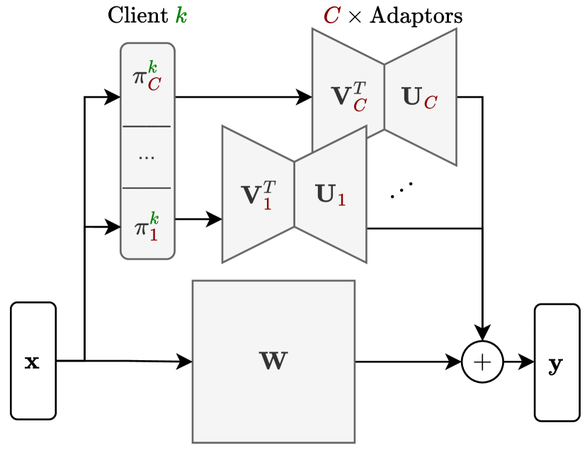
Thus, instead of regularizing the complexity of a personalized model by its proximity to a reference solution or clustering full models, we explicitly parameterize the personalized models as having low-rank differences from the global model. This is done by introducing a small number of low-rank adaptors per layer and a mixture vector per client that mixes between those adaptors. Thus, it implicitly regularizes the personal models through a weight-sharing mechanism that enforces a low-rank difference from the global model. Our approach can be seen as a hybrid that 1) explicitly constrains the complexity of the difference (per layer) between the global model and the personalized model and 2) casts the problem of learning these differences as a multi-task learning problem via the local mixture vectors. The main benefit of this approach is that low-rank adaptors can also be federated, i.e., collaboratively learned, and the number of local personalization parameters per client is minimal. This means our approach can be efficiently employed in the cross-device setting as well.
Contributions
Here, we summarize our contributions:
-
1.
We propose the Federated Low-Rank Adaptive Learning (FLoRAL), an efficient and lightweight FL framework for personalization. It acts as an extension to multi-task learning algorithms that are specifically designed for FL.
-
2.
Perhaps counter-intuitively, we show experimentally that a model with a mixture of adaptors can beat a mixture of models, even though the number of parameters is significantly larger, e.g., 9x larger. Also, a model with a mixture of adaptors on stateless clients (e.g., see Section 5) can generalize better than a model with a dedicated fine-tuned adaptor on stateful clients. This is a perfect demonstration of the efficiency of FLoRAL and the benefits of collaborative learning.
-
3.
We release the code for this framework, which includes plug-and-play wrappers for PyTorch models (Paszke et al., 2019) that are as simple as
Floral(model, rank=8, num_clusters=4). We also provide minimal extensions of Flower client and server modules (Beutel et al., 2022), making the adoption of our method in practice and reproducing the experiments seamless and easy. -
4.
We run various experiments and ablation studies showing that our FLoRAL framework is efficient given resource constraints in terms of relative parameter increase.
-
5.
We provide the convergence rate for local SGD on a multi-task objective with learnable router and highlight the difficulties that arise from aggregation mismatch. We also provide an extended analysis in the appendix showing better variance reduction from weight sharing.
2 Related Work
Multi-task Learning
Our problem can be seen as a multi-task learning problem in which the solutions share a base model. The closest work to ours in this respect is FedEM (Marfoq et al., 2021), which works by assigning to each client a personalized mixture vector that mixes between a small number of full models such that each model solves one task. FedEM then proceeds with an algorithm based on expectation maximization. One problem is that their approach assumes that the full models should be mixed. In contrast, we assume that the mixed components are only the adaptors, which constitute a small fraction of the model and are thus much more efficient in terms of memory. Other related works on clustering include IFCA (Ghosh et al., 2020), FedSoft (Li et al., 2022), and Federated-Clustering (Werner et al., 2023). The main difference from our work is that we only cluster a small component of the whole model, allowing the clients to benefit from having a shared base model that is learned among all the clients.
Personalization
Another approach to personalization is by introducing a proximal regularizer with respect to a reference model. Ditto (Li et al., 2021a) is a stateful algorithm that trains the local models by solving a proximal objective with respect to a reference model. The reference model is the FedAvg solution, which is attained concurrently by solving the non-regularized objective. Meta-learning approaches, inspired by Finn et al. (2017), can extend naturally to personalization. For example, Fallah et al. (2020) propose to solve a local objective that is an approximate solution after one local gradient step. Meta-learning also assumes that the local solutions are close to the FedAvg solution as they mimic fine-tuning from the FedAvg solution in some sense. In our approach, we do not assume that the clients are stateful nor that the FedAvg solution is meaningful or close to any of the local solutions. We assume that the local models can benefit from collaboration but still allow for personalization via different mixtures, which is much more memory efficient and can be managed by the server.
LoRA
Using mixture of LoRAs in FL is not new due to their popularity. The idea of mixing LoRAs has been explored recently (Wu et al., 2024b) for language models. SLoRA (Babakniya et al., 2023) focuses on parameter-efficient fine-tuning after federated training and thus does not federate the adaptors. Both FedLoRA (Wu et al., 2024a) and pFedLoRA (Yi et al., 2024) assume that the LoRAs are not federated as well, where they both also introduce a specific two-stage algorithm to train those LoRAs. The federated mixture of experts (Reisser et al., 2021) trains an ensemble of specialized models, but they specialize in input rather than prediction. FedJETs (Dun et al., 2023) uses whole models as experts in addition to a pre-trained feature aggregator as a common expert that helps the client choose the right expert. Other works explore mixture of LoRAs (Zhu et al., 2023; Yang et al., 2024) for adaptation but in a different, non-collaborative context.
Representation Learning
3 Preliminary
Notation
We denote We reserve some indices for specific objects: is a superset index222We reserve the superset for clients and the subset for clusters. denoting the client with being the number of clients, and is a subset index denoting the cluster with being the number of clusters. The number of clients in cluster c is . The client sampling distribution is , or when given cluster . The number of samples in client is , and the total number of samples is . We will use bold lowercase characters to denote vectors, e.g., denotes a vector of parameters, and uppercase bold characters for matrices, e.g., denotes the adaptive layer. As a relevant example, the adaptive parameters can be written in vector form as , where is a vectorization operator. A simplex is such that and for all .
3.1 Federated Learning
Federated learning (FL) is a framework for training a model on distributed data sources while the data remains private and on-premise. Let be the number of clients and the local loss function for client be . The global objective is
| (FL) |
where is a client distribution with support . The functions can be stochastic as well.
The most straightforward algorithm for optimizing FL is FedAvg (McMahan et al., 2023), which proceeds in a cycle as follows: 1) send copies of the global model to the participating clients, 2) train the copies locally on the client’s data, and then 3) send back the copies and aggregate them to get the new global model.
The objective FL assumes that a single global model can obtain an optimal solution that works for all the objectives, which is often not feasible due to heterogeneities in data distribution and system capabilities (Kairouz et al., 2021). A natural approach would be to consider personalized solutions for each client , an approach called PersonalizedFL (PFL).
| (PFL) |
Without the regularizer , the objective would simply amount to local independent training for each client, so clients do not benefit from collaboration and can suffer from a low availability of data. Adding the regularizer helps introduce a collaboration incentive or inductive bias. For example, Ditto has , where is the solution of FL, which implies that the personalized solutions should stay close to the FL solution.
The Ditto (Li et al., 2021a) objective still assumes that a single global solution is a good enough center for all clients, which can be limiting and impractical for real-world heterogeneous problems. Given a proximal regularization, an improvement on this assumption would be to introduce more than one center or cluster, such that clients belonging to some cluster are close to its center. The problem of finding the cluster centers is called Clustered FL (CFL).
Let be the number of ground-truth clusters and assume that it is known. Let be the client sampling distribution of cluster . We can reformulate the objective to account for clusters as follows
| (CFL) |
We can generalize the previous objectives under one objective by introducing (learnable) client mixtures for all with regularization , e.g. for weight sharing, which we denote as Mixed Federated Learning (MFL)
| (MFL) | ||||
| s.t. |
We can see that local losses from different clusters are mixed differently according to each client. From this formulation, the previous optimization problems can be recovered with the following settings
where is the indicator function.
Finally, in our formulation we use particular form of , where we split as and define
This weight-sharing across clients is based on the inductive bias that the optimal personalized solutions have low-complexity differences across the population (i.e., differences that could be explained in a parameter-efficient way). Therefore, in the rest of the paper, we do not use , but we replace it with explicit parametrization, where . We refer to as adaptors. The final objective, which we call MFL with Weight Sharing (MFL-WS), is of the form
| (MFL-WS) | ||||
| s.t. |
In the next section, we discuss the particular choice of adaptors.
3.2 Parameter-Efficient Adaptors
Linear layer
This LoRA was introduced in (Hu et al., 2021). Let be the base linear layer. We introduce a low-rank adaptive layer with rank , where and . We initialize such that is random (or initialized similarly to ) and is zero. The low-rank adaptive layer is
| (1) |
Relative parameter budget
It is easy to see that the number of parameters in a linear LoRA is , which can be much smaller than for small . We can have a constraint on the number of parameters relative to the model size, i.e., , where is the relative parameter budget per adaptor (e.g., for a maximum of 1% increase in model size per adaptor). Given a specific based on system capabilities, can be automatically set to be the maximum such that , or just . Note how attains its largest values when , where the equation simply becomes . We hereafter refer to as the budget (per adaptor), and set it to either 1% or 10% in the experiments. Note that for certain models, it is impossible to satisfy the budget if , so we enforce a minimum rank of 1 (otherwise, there will be no adaptors).
Convolution layer
Consider a 2D convolution layer. Let be the base convolution layer. We similarly introduce a “low-rank” adaptive convolution layer with rank , such that the adaptive convolution becomes , where is the convolution operator. We call these adaptive layers Convolution LoRAs (ConvLoRAs), which are more general than a linear LoRA on a matricized convolution as is often done in practice, e.g., in the official implementation (Hu et al., 2021).
We can have more than one way of defining and . Note that one of the convolutions in the adaptor should share the same padding, stride, and dilation as the base convolution, while the other should be such that it does not change the resolution of the input. Depending on what is meant by “rank” for convolution layers, we can either reduce the rank channel-wise, filter-wise, both, or as a linear layer by matricizing the convolution. We discuss these in detail in Section F.1 and show that a novel channel+filter-wise implementation is more parameter-efficient and performs better. More details about low-rank constructions of convolution layers can be found in (Jaderberg et al., 2014; Khodak et al., 2022).
Bias
Biases are vectors, so a low-rank parameterization would not be possible, and there is no straightforward way to have a parameter-efficient adaptor except by considering weight-sharing or a single constant. Due to biases contributing a small percentage of the overall number of parameters in large models, we consider adaptive biases as with extra biases initialized to 0. Although this adaptor is not parameter-efficient relative to , the small impact on the overall parameter count means that this is not a significant limitation. Moreover, as demonstrated in Section G.3, this approach can be crucial for achieving optimal accuracy.
4 Analysis for (MFL)
In order to connect the analysis with our FLoRAL framework, we can consider a vector parameterization of the model given client and cluster as in MFL-WS. Namely, we have , where it is understood as the concatenation of the two vectors and we emphasize that does not depend on the cluster. For example, can be the base layer and can be the LoRA adaptor. The analysis proceeds without assumptions on the form of . In Appendix B, we show the benefits of weight-sharing under suitable assumptions that make use of such a structure.
Recall the ground-truth router of client . In general, the probability of sampling a single client is often chosen to be proportional to the number of its data points, i.e., (note this is different from sampling a cohort, which is explained below). On the other hand, the probability that client samples cluster is by construction. Since we have , we can divide by to get . Overall, we have by construction and by assumption, so that
| (2) |
Thus, we use the per-cluster aggregator since we aggregate variables per cluster, e.g., aggregate across clients.
We now introduce notations for the analysis. Denote the learned estimate of at iteration . Denote and similarly . Define the aggregation operators and . Additionally, we denote using the same aggregation operators but taken with respect to and , respectively.
Recall that the mixed (or personalized) objective of client is . The objective MFL can be stated more succinctly as
| (3) |
Remark 4.1.
Consider a cluster assignment router (i.e., one-hot w.r.t. ). Let and be its associated cluster. Then, and .
Local SGD
With the above notation in hand, we consider the local SGD setting (Stich, 2019). We note that our work is orthogonal to (Wang & Ji, 2024) since they can estimate with an unbiased participation indicator variable, whereas we assume that is known and estimate instead, which itself cannot be unbiased because of the dependency of the estimate on the optimal objective values. Further, the analysis Pillutla et al. (2022) cannot be directly adapted because it is concerned with a split of global and local variables (i.e., weights and mixture, respectively), whereas we take into account weight sharing across clusters and train mixtures explicitly. Thus, we follow the generic local SGD framework with perturbed iterates and demonstrate the benefits of our parameterization where applicable.
For client and cluster , the algorithm starts with the initialization with , without loss of generality. We define the aggregated gradient as for independently sampled clients every steps, i.e., for all where . Though similar, we will explicitly reserve the random variables for denoting sampled clients at time and for denoting a “tracking” variable of the expected performance over clients, which will be independent of . Let and define . Assume an unbiased estimate , where we denote the expectation with respect to given . Let be any point satisfying . We run gradient steps with a learning rate . Synchronization happens every iterations so that , such that . The algorithm we use in the analysis is the following
| (4) | ||||
| (5) |
All of the practical implementation details will be discussed in more detail in the next section.
Following the local SGD analysis in (Stich, 2019), we make the following corresponding assumptions.
Assumption 4.2 (-smoothness and -strong convexity).
is -smooth and -strongly convex. In other words, , the following holds
| (6) | ||||
| (7) |
Assumption 4.3 (Bounded second moment).
, , .
Assumption 4.4 (Bounded variance).
, , .
The main quantity of interest in our analysis is the total variation distance where . We may also refer to it as the aggregation mismatch, or just mismatch.
Using the router update in 5, we can obtain the convergence bound of local SGD but with an extra term and a learning rate inversely proportional to instead of . This seems to be unavoidable without extra assumptions due to a circular dependency between and . However, we show in Corollary A.5 that local SGD descent is recovered when . The convergence rate for this general case can be seen in Theorem A.9.
Here, we present a convergence bound given an assumption on the decrease of . The exact bound can be found in Theorem A.10. We defer all proofs to Appendix A.
Theorem 4.5.
Consider the setup in Section 4. Let , , and . Initialize for all , and assume for all . Assume that without loss of generality, and assume that for . Let with and . Then,
| (8) |
Observe that we recover local SGD asymptotically when and (which is the case for FL), or when since . Observe also that we obtain a general notion of variance reduction through . Indeed, in the FL case and for cluster in the CFL case, where is the number of clients in cluster .
Note that for balanced clustered FL problems, but this can become as low as when a cluster contains one client. The difficulty is inherent for such edge cases, but the dependence on in the bound appears only in higher-order terms (see Theorem A.10 for the full bound). We believe that having independent learning rates per client should remove the in , and a finer analysis on the quantity can bound further from below, but we leave this for future work.
In Appendix B, we extend the analysis to the FML case with weight sharing (explained in the next section). Given fine-grained variances and cluster heterogeneity conditions for which weight sharing works best, we can demonstrate better variance reduction of the base layer under a trade-off with cluster heterogeneity (see 33, for example). A better understanding of weight sharing and the assumptions in Appendix B is an interesting direction for future work.
5 Practical Implementation
Mixture of adaptors
The (MFL) objective suggests that any learning algorithm will have to run at least forward passes per step for each client, which is necessary for computing the objective. One way to circumvent that is by “moving” the mixture inside the objective. This allows us to mix the weights and perform one forward pass. We call this Federated Mixture Learning (FML)333The “M” in the acronym follows the position of the mixture in the objective.
| (FML) | ||||
| s.t. |
Observe that for convex , this proxy acts as a lower bound since due to Jensen’s inequality. Thus, for convex losses , minimizing MFL implies minimizing FML, but not vice versa. In this sense, FML could be seen as a more general problem, and MFL is a relaxation. We note that this problem is similar to FedEM (Marfoq et al., 2021), but we only use mixture vectors of size and we do not have sample-specific weights.
This formulation is especially useful for additive adaptors since the weights can be merged into one. Also, it allows us to mix the adaptors and run one forward pass, which is often more efficient than running forward passes. This is particularly true for inference, in which the weights can be merged once so that forward passes come without extra cost. The benefits of weight sharing can also manifest through better variance reduction, which is demonstrated in Appendix B.
Learning the mixture weights
Instead of optimizing directly in , we consider the parameterization for some vector , i.e., .
Note that is a local parameter and not aggregated. The cost of storing in each client is minimal as it is of size , which is often significantly small compared to the model size . Even if we consider stateless clients, the server should be able to handle an extra storage and communication budget of , which is . Note that the server does not need to know the IDs of the clients and that the clients can learn the from scratch every round, as it is not expensive. Let us consider a scenario where the cost is prohibitive. Suppose the model size is and the client participation ratio is . The extra cost for the server will be for . Thus, the prohibitive scenario occurs only when , which is often not the case as is rarely this small (e.g., a 32 by 32 linear layer with bias has more 1000 parameters), let alone . The only drawback with stateless clients is the need to learn from scratch every round, which is cheap to learn given the current model.
In Appendix C, we make a connection between the router update in 5 for (MFL) and the gradient descent update of on (FML) under the Softmax parameterization, and show conditions under which they become equivalent.
FLoRAL problem and algorithm
We obtain the FLoRAL problem by employing the weight sharing regularizer in (MFL-WS) to (FML) and using low-rank adaptors . Weight sharing and low-rankedness are explicit in the parameterization.
The algorithm we use to solve (FLoRAL) in practice is shown in Algorithm 1 and is straightforward. We use simultaneous gradient descent for and , so we simply write the update in terms of the concatenation . One trick we employ to ensure better convergence is LoRA preconditioning, which is detailed in Appendix D.
6 Experiments
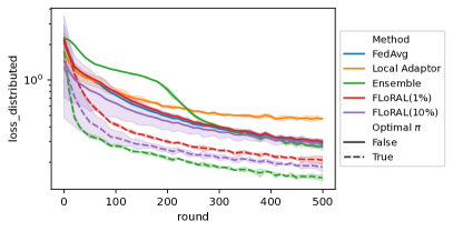
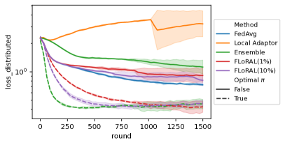
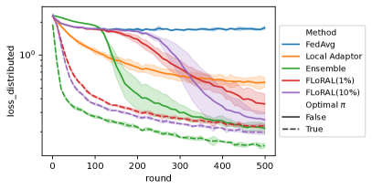
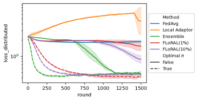
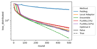
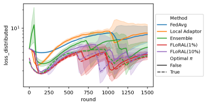
In this section, we empirically show the performance of our lightweight framework. In particular, we show that our FLoRAL framework, which can have as few as extra parameters, can possibly outperform an ensemble of models, which can collectively have up to extra parameters. It can also outperform clients equipped with a local adaptor. This clearly shows the benefit of collaborative learning and how personalization and adaptation can also be done efficiently in a collaborative setting.
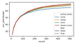
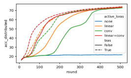
We consider datasets with known ground-truth clusters, for example, linear and MLP synthetic datasets, MNIST and CIFAR-10 with rotation or label shift Ghosh et al. (2020); Werner et al. (2023), CIFAR-100 with 10 clusters, each having 10 unique labels (Werner et al., 2023). Further, we consider the same datasets with only 5% data availability per client (with 10 being the minimum number of samples per client). This is to demonstrate the benefits of our approach, which would be when a large model might overfit the local datasets. The results can be seen in Table 1. Further ablation studies on and , the adaptors, and the type of ConvLoRAs can be found in Table 3, Table 5, and Table 5, respectively.
In general, we follow the experimental setup in (Werner et al., 2023) or (Pillutla et al., 2022) and implement our experiments using PyTorch (Paszke et al., 2019) and Flower (Beutel et al., 2022). We use the simplest setup possible without any tricks other than LoRA preconditioning, which is explained in Appendix D. We discuss another trick called LoRA centering in Appendix E, which we believe is potentially useful but is still in the experimental phase. The algorithm we use in practice is shown in Algorithm 1. Further details can be found in Appendix G.
We emphasize that we do not aim to improve over the state-of-the-art. However, we can refer readers to (Werner et al., 2023) for a relevant comparison, where we should note that the algorithm they use has a quadratic running time in the number of clients. We implemented and tested their linear-time momentum-based algorithm, but it suffers from cluster collapse on our synthetic tasks.
| Method | MNIST | CIFAR-10 | CIFAR-100 | ||||||||
|---|---|---|---|---|---|---|---|---|---|---|---|
| Full | Reduced | Full | Reduced | Full | Reduced | ||||||
| R | LS | R | LS | R | LS | R | LS | ||||
| FedAvg | 91.5 0.6 | 25.8 2.4 | 78.2 0.6 | 23.2 0.9 | 64.4 0.3 | 21.9 0.4 | 45.6 0.3 | 18.7 0.4 | 29.2 1.8 | 20.7 1.4 | |
| Local Adaptor | 86.6 0.3 | 84.5 1.8 | 47.4 5.4 | 32.0 2.3 | 66.3 0.5 | 68.8 0.5 | 33.5 0.5 | 30.8 0.8 | 85.1 0.8 | 39.5 2.8 | |
| Ensemble | ✗ | 92.0 0.1 | 93.8 0.5 | 66.7 5.3 | 86.4 0.4 | 71.0 2.8 | 46.4 9.2 | 42.4 0.9 | 41.7 4.6 | 86.2 0.0 | 43.7 3.2 |
| Ensemble | ✓ | 95.8 0.3 | 95.6 0.3 | 88.2 1.4 | 87.6 1.3 | 73.7 0.2 | 73.3 0.1 | 45.0 0.9 | 45.1 0.8 | 92.8 0.3 | 55.0 0.4 |
| FLoRAL(1%) | ✗ | 91.3 0.6 | 89.7 3.2 | 73.1 3.7 | 46.0 9.9 | 65.5 0.4 | 62.8 8.8 | 45.2 0.3 | 44.2 0.9 | 81.3 0.5 | 52.2 0.5 |
| FLoRAL(1%) | ✓ | 93.9 0.8 | 93.7 0.2 | 87.5 2.1 | 87.6 0.5 | 68.9 0.2 | 72.2 0.2 | 47.8 0.9 | 44.1 0.6 | 82.4 0.2 | 53.1 0.4 |
| FLoRAL(10%) | ✗ | 91.8 1.0 | 93.1 0.9 | 75.7 2.3 | 70.8 7.1 | 65.1 0.3 | 56.2 5.5 | 44.5 0.4 | 42.1 0.2 | 87.3 0.3 | 51.2 1.0 |
| FLoRAL(10%) | ✓ | 94.5 0.6 | 94.2 0.2 | 87.0 0.7 | 86.9 0.5 | 69.3 0.5 | 72.1 0.5 | 47.2 0.3 | 42.7 0.3 | 86.6 0.5 | 53.9 0.9 |
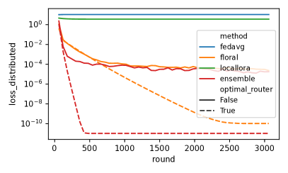
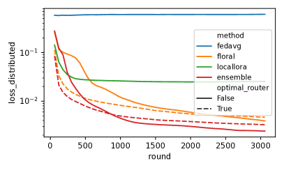
Synthetic
Consider a regression task where we want to learn given , where . We construct two versions of this regression task: one is based on a linear model plus a personalized LoRA, and the other is based on a similar setup on the first layer of a two-layer ReLU net. This dataset provides a proof of concept for our method. Namely, the target model for client is
| (9) |
where , , , and . Similarly, consider the 2-layer ReLU neural net for , where we write the ReLU function as . We discuss these datasets in more detail in Section G.1. The results in Table 3 show the performances with and for the linear version and and for the MLP version. Note that even the linear task is not easy to solve, and similar problems have been studied in the mixed linear regression literature, e.g., see (Chen et al., 2021).
| CIFAR-10 | CIFAR-100 | |||
|---|---|---|---|---|
| R | LS | |||
| 1% | 66.5 | 36.3 | 48.8 | |
| 10% | 66.8 | 41.6 | 50.9 | |
| 1% | 70.2 | 74.1 | 51.7 | |
| 10% | 71.5 | 74.2 | 57.4 | |
| 1% | 69.0 | 73.8 | 51.3 | |
| 10% | 70.8 | 74.1 | 54.8 | |
MNIST and CIFAR-10
We test our method on a clustered version of MNIST and CIFAR-10 datasets in which the clusters are generated according to one of the following tasks: 1) a rotation task, where each cluster rotates the image by degrees, and 2) a label shift task, where cluster shifts the labels by . Following (Werner et al., 2023), we choose and for MNIST and sample of the clients every round, and choose and for CIFAR-10 and sample all clients every round. The model for MNIST is a 2-layer ReLU net, whereas for CIFAR-10, it has two convolution layers followed by a 2-layer ReLU net classifier.
CIFAR-100
The CIFAR-100 task is to train a model that is not expressive enough to fit 100 labels yet expressive enough to fit 10 labels. Thus, we expect that the model would benefit from collaboration with the right clients. The setup is to divide the 100 labels into clusters such that each cluster has 10 unique labels and then split each cluster uniformly into clients (so, in total, ). The model used is VGG-8, a custom-sized model from the VGG-family (Simonyan & Zisserman, 2015) that is specifically able to fit 10 labels but not 100. We sample 25 clients every round, which makes the task harder than (Werner et al., 2023) and can result in overfitting.
Discussion
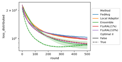
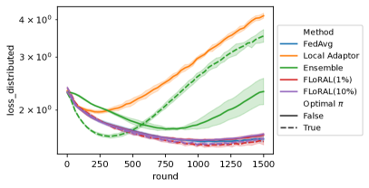
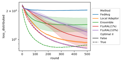
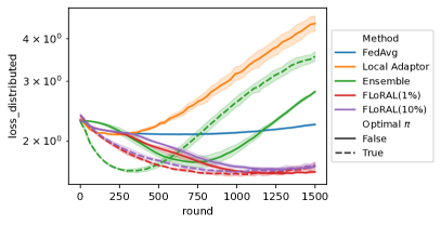
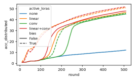
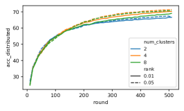
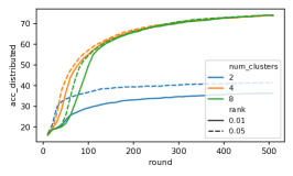
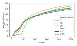
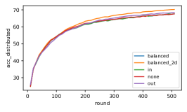
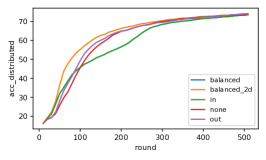
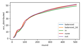
The results in Figure 8 show the robustness of FLoRAL with respect to its hyperparameters, particularly when is larger than the number of ground-truth clusters. As for Table 1, we can see that FLoRAL is always competitive with the best baseline, which is ensembles with optimal routers. A particularly interesting case is the reduced CIFAR-10-R experiments, in which FLoRAL(1%) and FLoRAL(10%) surprisingly outperform ensembles even in the optimal routing case, which seems slightly counter-intuitive. We believe this to be due to the variance reduction shown in Appendix B. Note that FLoRAL() has extra parameters, whereas ensembles have . For example, when and , FLoRAL(1%) adds parameters vs. for ensembles, and when , it is vs. . Local Adaptors require each client to have its own adaptor (i.e., each client has a storage of size ). Regardless of its feasibility, FLoRAL is shown to leverage the power of collaboration when local adaptors fail to do so. We note that the low accuracies of FLoRAL with learned routing in reduced MNIST-LS can be alleviated with more training rounds, e.g., see Section G.5 for plots. Overall, these results demonstrate that FLoRAL is an efficient personalization method, and it can lead to better generalization in low-data regimes.
7 Conclusion
In this work, we presented a parameter-efficient method for collaborative learning and personalization. Here are some future directions we are interested in exploring:
-
•
Is there a principled way to understand the trade-off between parameter-efficiency and the accuracy gains from increasing or and how to choose them in practice?
-
•
FML can be formulated as a “multimodal optimization” problem (Wong, 2015), which can also be described in terms of a model class that uses mixture-candidate distributions (Khan & Rue, 2023). It would be interesting to explore the design of efficient algorithms under their framework, e.g., with a mixture of structured distributions (Louizos & Welling, 2016).
-
•
Our framework is suitable for federated fine-tuning of language models. We are interested in exploring this direction.
-
•
The router can route based on its input, as in mixture of experts (Shazeer et al., 2017). It can also be learned per layer. Preliminary experiments suggest that these tweaks provide marginal benefits, but there is still room for exploration.
-
•
We are interested in designing methods for zero-shot generalization to unseen clients based on FLoRAL. Is it possible to fine-tune the router without labels?
References
- Aghajanyan et al. (2020) Armen Aghajanyan, Luke Zettlemoyer, and Sonal Gupta. Intrinsic dimensionality explains the effectiveness of language model fine-tuning. arXiv preprint arXiv:2012.13255, 2020.
- Almansoori et al. (2024) Abdulla Jasem Almansoori, Samuel Horváth, and Martin Takáč. PaDPaf: Partial disentanglement with partially-federated GANs. Transactions on Machine Learning Research, 2024. ISSN 2835-8856. URL https://openreview.net/forum?id=vsez76EAV8.
- Babakniya et al. (2023) Sara Babakniya, Ahmed Roushdy Elkordy, Yahya H. Ezzeldin, Qingfeng Liu, Kee-Bong Song, Mostafa El-Khamy, and Salman Avestimehr. Slora: Federated parameter efficient fine-tuning of language models, 2023.
- Beutel et al. (2022) Daniel J. Beutel, Taner Topal, Akhil Mathur, Xinchi Qiu, Javier Fernandez-Marques, Yan Gao, Lorenzo Sani, Kwing Hei Li, Titouan Parcollet, Pedro Porto Buarque de Gusmão, and Nicholas D. Lane. Flower: A friendly federated learning research framework, 2022.
- Beznosikov et al. (2021) Aleksandr Beznosikov, Vadim Sushko, Abdurakhmon Sadiev, and Alexander Gasnikov. Decentralized personalized federated min-max problems. arXiv preprint arXiv:2106.07289, 2021.
- Borodich et al. (2021) Ekaterina Borodich, Aleksandr Beznosikov, Abdurakhmon Sadiev, Vadim Sushko, Nikolay Savelyev, Martin Takáč, and Alexander Gasnikov. Decentralized personalized federated min-max problems. arXiv preprint arXiv:2106.07289, 2021.
- Chen et al. (2021) Yanxi Chen, Cong Ma, H. Vincent Poor, and Yuxin Chen. Learning mixtures of low-rank models. IEEE Transactions on Information Theory, 67(7):4613–4636, 2021. doi: 10.1109/TIT.2021.3065700.
- Chen et al. (2022) Zixiang Chen, Yihe Deng, Yue Wu, Quanquan Gu, and Yuanzhi Li. Towards understanding mixture of experts in deep learning. arXiv preprint arXiv:2208.02813, 2022.
- Cheng et al. (2021) Gary Cheng, Karan N. Chadha, and John C. Duchi. Fine-tuning is fine in federated learning. ArXiv, abs/2108.07313, 2021.
- Dun et al. (2023) Chen Dun, Mirian Hipolito Garcia, Guoqing Zheng, Ahmed Hassan Awadallah, Robert Sim, Anastasios Kyrillidis, and Dimitrios Dimitriadis. Fedjets: Efficient just-in-time personalization with federated mixture of experts, 2023.
- Fallah et al. (2020) Alireza Fallah, Aryan Mokhtari, and Asuman Ozdaglar. Personalized federated learning: A meta-learning approach, 2020.
- Finn et al. (2017) Chelsea Finn, Pieter Abbeel, and Sergey Levine. Model-agnostic meta-learning for fast adaptation of deep networks, 2017. URL https://arxiv.org/abs/1703.03400.
- Gao et al. (2022) Dashan Gao, Xin Yao, and Qiang Yang. A survey on heterogeneous federated learning, 2022.
- Ghosh et al. (2020) Avishek Ghosh, Jichan Chung, Dong Yin, and Kannan Ramchandran. An efficient framework for clustered federated learning. Advances in Neural Information Processing Systems, 33:19586–19597, 2020.
- Hu et al. (2021) Edward J. Hu, Yelong Shen, Phillip Wallis, Zeyuan Allen-Zhu, Yuanzhi Li, Shean Wang, Lu Wang, and Weizhu Chen. Lora: Low-rank adaptation of large language models, 2021.
- Jaderberg et al. (2014) Max Jaderberg, Andrea Vedaldi, and Andrew Zisserman. Speeding up convolutional neural networks with low rank expansions, 2014.
- Kairouz et al. (2021) Peter Kairouz, H. Brendan McMahan, Brendan Avent, Aurélien Bellet, Mehdi Bennis, Arjun Nitin Bhagoji, Kallista Bonawitz, Zachary Charles, Graham Cormode, Rachel Cummings, Rafael G. L. D’Oliveira, Hubert Eichner, Salim El Rouayheb, David Evans, Josh Gardner, Zachary Garrett, Adrià Gascón, Badih Ghazi, Phillip B. Gibbons, Marco Gruteser, Zaid Harchaoui, Chaoyang He, Lie He, Zhouyuan Huo, Ben Hutchinson, Justin Hsu, Martin Jaggi, Tara Javidi, Gauri Joshi, Mikhail Khodak, Jakub Konečný, Aleksandra Korolova, Farinaz Koushanfar, Sanmi Koyejo, Tancrède Lepoint, Yang Liu, Prateek Mittal, Mehryar Mohri, Richard Nock, Ayfer Özgür, Rasmus Pagh, Mariana Raykova, Hang Qi, Daniel Ramage, Ramesh Raskar, Dawn Song, Weikang Song, Sebastian U. Stich, Ziteng Sun, Ananda Theertha Suresh, Florian Tramèr, Praneeth Vepakomma, Jianyu Wang, Li Xiong, Zheng Xu, Qiang Yang, Felix X. Yu, Han Yu, and Sen Zhao. Advances and open problems in federated learning, 2021.
- Khan & Rue (2023) Mohammad Emtiyaz Khan and Håvard Rue. The bayesian learning rule, 2023.
- Khodak et al. (2022) Mikhail Khodak, Neil Tenenholtz, Lester Mackey, and Nicolò Fusi. Initialization and regularization of factorized neural layers, 2022.
- Li et al. (2022) Chengxi Li, Gang Li, and Pramod K. Varshney. Federated learning with soft clustering. IEEE Internet of Things Journal, 9(10):7773–7782, 2022. doi: 10.1109/JIOT.2021.3113927.
- Li et al. (2018) Chunyuan Li, Heerad Farkhoor, Rosanne Liu, and Jason Yosinski. Measuring the intrinsic dimension of objective landscapes. arXiv preprint arXiv:1804.08838, 2018.
- Li et al. (2021a) Tian Li, Shengyuan Hu, Ahmad Beirami, and Virginia Smith. Ditto: Fair and robust federated learning through personalization. In International conference on machine learning, pp. 6357–6368. PMLR, 2021a.
- Li et al. (2021b) Xiaoxiao Li, Meirui Jiang, Xiaofei Zhang, Michael Kamp, and Qi Dou. Fedbn: Federated learning on non-iid features via local batch normalization, 2021b.
- Louizos & Welling (2016) Christos Louizos and Max Welling. Structured and efficient variational deep learning with matrix gaussian posteriors. In Maria Florina Balcan and Kilian Q. Weinberger (eds.), Proceedings of The 33rd International Conference on Machine Learning, volume 48 of Proceedings of Machine Learning Research, pp. 1708–1716, New York, New York, USA, 20–22 Jun 2016. PMLR. URL https://proceedings.mlr.press/v48/louizos16.html.
- Marfoq et al. (2021) Othmane Marfoq, Giovanni Neglia, Aurélien Bellet, Laetitia Kameni, and Richard Vidal. Federated multi-task learning under a mixture of distributions. In M. Ranzato, A. Beygelzimer, Y. Dauphin, P.S. Liang, and J. Wortman Vaughan (eds.), Advances in Neural Information Processing Systems, volume 34, pp. 15434–15447. Curran Associates, Inc., 2021. URL https://proceedings.neurips.cc/paper_files/paper/2021/file/82599a4ec94aca066873c99b4c741ed8-Paper.pdf.
- McMahan et al. (2023) H. Brendan McMahan, Eider Moore, Daniel Ramage, Seth Hampson, and Blaise Agüera y Arcas. Communication-efficient learning of deep networks from decentralized data, 2023.
- Mishchenko et al. (2023) Konstantin Mishchenko, Rustem Islamov, Eduard Gorbunov, and Samuel Horváth. Partially personalized federated learning: Breaking the curse of data heterogeneity, 2023.
- Nguyen et al. (2022) A. Tuan Nguyen, Philip Torr, and Ser-Nam Lim. Fedsr: A simple and effective domain generalization method for federated learning. In Alice H. Oh, Alekh Agarwal, Danielle Belgrave, and Kyunghyun Cho (eds.), Advances in Neural Information Processing Systems, 2022. URL https://openreview.net/forum?id=mrt90D00aQX.
- Paszke et al. (2019) Adam Paszke, Sam Gross, Francisco Massa, Adam Lerer, James Bradbury, Gregory Chanan, Trevor Killeen, Zeming Lin, Natalia Gimelshein, Luca Antiga, Alban Desmaison, Andreas Köpf, Edward Yang, Zach DeVito, Martin Raison, Alykhan Tejani, Sasank Chilamkurthy, Benoit Steiner, Lu Fang, Junjie Bai, and Soumith Chintala. Pytorch: An imperative style, high-performance deep learning library, 2019.
- Pillutla et al. (2022) Krishna Pillutla, Kshitiz Malik, Abdel-Rahman Mohamed, Mike Rabbat, Maziar Sanjabi, and Lin Xiao. Federated learning with partial model personalization. In Kamalika Chaudhuri, Stefanie Jegelka, Le Song, Csaba Szepesvari, Gang Niu, and Sivan Sabato (eds.), Proceedings of the 39th International Conference on Machine Learning, volume 162 of Proceedings of Machine Learning Research, pp. 17716–17758. PMLR, 17–23 Jul 2022. URL https://proceedings.mlr.press/v162/pillutla22a.html.
- Rakhlin et al. (2012) Alexander Rakhlin, Ohad Shamir, and Karthik Sridharan. Making gradient descent optimal for strongly convex stochastic optimization. In Proceedings of the 29th International Coference on International Conference on Machine Learning, ICML’12, pp. 1571–1578, Madison, WI, USA, 2012. Omnipress. ISBN 9781450312851.
- Reisser et al. (2021) Matthias Reisser, Christos Louizos, Efstratios Gavves, and Max Welling. Federated mixture of experts, 2021.
- Sadiev et al. (2022) Abdurakhmon Sadiev, Ekaterina Borodich, Aleksandr Beznosikov, Darina Dvinskikh, Saveliy Chezhegov, Rachael Tappenden, Martin Takáč, and Alexander Gasnikov. Decentralized personalized federated learning: Lower bounds and optimal algorithm for all personalization modes. EURO Journal on Computational Optimization, 10:100041, 2022.
- Shazeer et al. (2017) Noam Shazeer, Azalia Mirhoseini, Krzysztof Maziarz, Andy Davis, Quoc Le, Geoffrey Hinton, and Jeff Dean. Outrageously large neural networks: The sparsely-gated mixture-of-experts layer, 2017.
- Simonyan & Zisserman (2015) Karen Simonyan and Andrew Zisserman. Very deep convolutional networks for large-scale image recognition, 2015.
- Stich (2019) Sebastian U. Stich. Local sgd converges fast and communicates little, 2019.
- Stich et al. (2018) Sebastian U Stich, Jean-Baptiste Cordonnier, and Martin Jaggi. Sparsified sgd with memory. Advances in neural information processing systems, 31, 2018.
- Tan et al. (2022) Yue Tan, Guodong Long, Lu Liu, Tianyi Zhou, Qinghua Lu, Jing Jiang, and Chengqi Zhang. Fedproto: Federated prototype learning across heterogeneous clients, 2022. URL https://arxiv.org/abs/2105.00243.
- Tong et al. (2021) Tian Tong, Cong Ma, and Yuejie Chi. Accelerating ill-conditioned low-rank matrix estimation via scaled gradient descent. Journal of Machine Learning Research, 22(150):1–63, 2021.
- Wang & Ji (2024) Shiqiang Wang and Mingyue Ji. A lightweight method for tackling unknown participation statistics in federated averaging, 2024. URL https://arxiv.org/abs/2306.03401.
- Wang et al. (2023) Yanmeng Wang, Qingjiang Shi, and Tsung-Hui Chang. Why batch normalization damage federated learning on non-iid data?, 2023.
- Werner et al. (2023) Mariel Werner, Lie He, Sai Praneeth Karimireddy, Michael Jordan, and Martin Jaggi. Provably personalized and robust federated learning. Transactions on Machine Learning Research, 2023.
- Wong (2015) Ka-Chun Wong. Evolutionary multimodal optimization: A short survey, 2015. URL https://arxiv.org/abs/1508.00457.
- Wu et al. (2024a) Xinghao Wu, Xuefeng Liu, Jianwei Niu, Haolin Wang, Shaojie Tang, and Guogang Zhu. FedloRA: When personalized federated learning meets low-rank adaptation, 2024a. URL https://openreview.net/forum?id=bZh06ptG9r.
- Wu et al. (2024b) Xun Wu, Shaohan Huang, and Furu Wei. MoLE: Mixture of loRA experts. In The Twelfth International Conference on Learning Representations, 2024b. URL https://openreview.net/forum?id=uWvKBCYh4S.
- Yang et al. (2024) Yuqi Yang, Peng-Tao Jiang, Qibin Hou, Hao Zhang, Jinwei Chen, and Bo Li. Multi-task dense prediction via mixture of low-rank experts. In Proceedings of the IEEE/CVF Conference on Computer Vision and Pattern Recognition (CVPR), pp. 27927–27937, June 2024.
- Yi et al. (2024) Liping Yi, Han Yu, Gang Wang, Xiaoguang Liu, and Xiaoxiao Li. pfedlora: Model-heterogeneous personalized federated learning with lora tuning, 2024.
- Zhang & Pilanci (2024) Fangzhao Zhang and Mert Pilanci. Riemannian preconditioned lora for fine-tuning foundation models, 2024.
- Zhang et al. (2023) Hao Zhang, Chenglin Li, Wenrui Dai, Junni Zou, and Hongkai Xiong. Fedcr: personalized federated learning based on across-client common representation with conditional mutual information regularization. In Proceedings of the 40th International Conference on Machine Learning, ICML’23. JMLR.org, 2023.
- Zhu et al. (2023) Yun Zhu, Nevan Wichers, Chu-Cheng Lin, Xinyi Wang, Tianlong Chen, Lei Shu, Han Lu, Canoee Liu, Liangchen Luo, Jindong Chen, and Lei Meng. Sira: Sparse mixture of low rank adaptation, 2023. URL https://arxiv.org/abs/2311.09179.
Appendix A Proofs
We reiterate the notations part from the main text here for clarity. Let and . Define the expectation operators and and similarly for their estimates and . We drop from the notation for clarity. We use the variable to denote client sampling, and should be understood as randomness in client sampling given cluster , for example. Finally, let the global function of cluster be . Note the absence of in the weight.
The analysis roughly follows (Stich, 2019) and differ mostly in the appearance of the total variation distance between and .
We start by introducing virtual iterates for tracking the aggregated weights (or gradients) with respect to the true router (or the estimated router) at every time step, which will be mainly useful for the analysis. These iterates coincide at the synchronization step, in which they become equal by construction of the algorithm. The iterates are as follows
| (10) | |||
| (11) |
Note that and . Hence, using , we have
| (12) |
In the original local SGD analysis, the correlation error is 0 since we aggregate the sampled gradients exactly and thus the expectation gives . Note that the expectation is implicitly defined , which would be , where since (because we sample clients every round).
A.1 Bounding descent
Lemma A.1 (Descent bound 1).
Given the setting and the assumptions in Section 4, the following holds
Proof.
From the ideal aggregation descent, we have
where we have used Jensen’s inequality 444 for random variable and convex .. As for the correlation error, we can write it as
We bound with Young’s inequality 555 for .
where we have used Jensen’s inequality as before.
Adding everything together, we get
Observe that, by 4.2 and , we have
| (13) |
and
| (14) |
We bound with Young’s inequality
We now plug in the results into the main bound
where we have used Jensen’s inequality . This completes the proof.
∎
Lemma A.2 (Gradient aggregation error).
Let and . Then,
| (15) |
Proof.
We divide the gradient aggregation error into controllable terms.
| (16) |
The first term can be bounded by noting for independent , which holds since we condition on the previous iterates. We use 4.4 to obtain
| (17) |
Lemma A.3 (Weights second moment).
Assume that and , where , i.e., . Then, we have
Proof.
Let and recall that by synchronization we have . Using with , we get
| (19) | ||||
where 19 uses and . Note that the bound for follows using the same argument. The assumption about the learning rate implies that it does not decay by more than some factor (e.g., ) before the next synchronization, which can be easily satisfied by adding in the denominator of . ∎
Lemma A.4 (Descent bound 2).
Assume that and , where and defined as in Lemma A.2. Then,
Proof.
The bound follows from applying Lemmas A.2 and A.3 on Lemma A.1. ∎
Discussion
Let us stop here and compare this bound with that of vanilla local SGD. First, we observe that we retrieve the original variance reduction (up to a constant factor). Next, we see that the directly incurred cost from aggregation mismatch is . The aggregation mismatch also manifests in the optimality gap in the sense that it “dampens” the guarantee as the aggregation increases, which we will make more precise later.
In general, the descent lemma above can recover local SGD’s descent lemma in the FL setting, which immediately implies its convergence rate.
Corollary A.5.
Proof.
Since in local SGD, this trivially gives “uniform” routing and thus , i.e., . Note that we have used the same assumptions, so we can apply Lemma A.4 with to obtain the descent lemma of local SGD up to constant factors (and up to application of Lemmas A.2 and A.3). ∎
Next, we want to bound the quantity given the update 5, and relate the new bound to Lemma A.4. After that, we can derive the convergence rate with the help of a technical lemma. We also derive the convergence rate given a slow decay assumption on , which shows more clearly the effect of aggregation mismatch on convergence.
A.2 Bounding the total variation distance
The following bound follows from the router update in 5.
Lemma A.6 (Total variation distance bound).
Consider the choice , and assume that we can write , where is bounded below by 0 and , . Then,
Proof.
Let . We will consider the cases where and separately.
Case :
Let be the partition function of client , so that we can write . Recall that , and let be the partition function of cluster . Equivalently define and to be the partition functions of client and cluster give the optimal router , respectively. Observe
| (20) |
where we have used Pinsker’s inequality, the router’s expression, and .
Using , we can write
| () |
and using similar arguments, we can show that
| () |
By properties of the LogSumExp function, we have
and similarly with and . Observe that and since the uniform case has the lowest max probability. Now define the centered function and note that . Adding and subtracting to both terms in () and using the expressions above, we can get
| () |
Combining () and (), we get
where the second inequality follows because . Applying this inequality to the overall bound 20, we have
| (21) |
Case :
Note that by 5, so we get the same bound 21 but in terms of . If we decompose the function gap , we see that it suffices to bound the first term to be able to write in terms of function gap at step . We can also take the expectations out since neither nor depend on .
We complete the proof by taking the max of both cases, which simply amounts to adding both cases. ∎
The following descent lemma will be used to get the convergence rate without any assumptions on other than what we have in the router update 5.
Lemma A.7 (Descent bound 3).
Let the conditions in Lemmas A.4 and A.6 be satisfied. Without loss of generality, assume that . If , where , then
Proof.
We apply Lemma A.6 on Lemma A.4 and rearrange to get
In order to have a meaningful convergence of the optimality gap, we have to bound it from above, so we should have
| (22) |
for some .
Suppose , and recall that is given, so we fix it. Write . Then, , so that 22 becomes . If we set for some , we would have , implying that
Setting gives , where is some strict upper bound of for all , but we should also have . Thus, we set , getting
| (23) |
Now, if with for some , 22 would imply , so that gives but under the condition . Thus, setting gives the same setting in 23 with 1 instead of . Thus, for all , we should have
We can restrict the denominator to without loss of generality. Then, we can upper bound , so that suffices for this choice.
Overall, we have , and using 22 with , we get
Given our choice of , we note that , which completes the proof. ∎
Discussion
Note that the learning rate is not as strict as it may look. First of all, note that is the case of interest, as otherwise, . Taking the minimum for such that makes sense because , so .
Now assume that for all . The lowest value can attain is when and is very small. This can happen, for example, when a cluster has one client. However, a uniform initialization for the routers would have that
Since , we would then have since we assumed .
Suppose . If , i.e., the number of clients in cluster is 1, then we cannot improve any further. This can be even worse if there is one data point for client . However, these extreme heterogeneity scenarios are inherently difficult, so it is better to capture this heterogeneity with some term, particularly when , which follows from .
For example, assume that for all such that , so that . In other words, we can choose . This implies that .
The value is a uniformity measure, so that a larger denotes a more uniform allocation of clients in cluster . For example, if , then, for all such that , we have . On the other hand, if , then it is possible for some clients to have , or in the worst case, when only one client is in cluster (remember that clients with are ignored). When cluster sizes are comparable, we have , meaning that .
Thus, in general, with uniform router initialization and when (which is a mild restriction to ensure is smaller than ), we have
| (24) |
Regarding the operator in , it is only required because it is a uniform learning rate for all clients, so it must converge for the worst client, which is the client with the least amount of data (i.e., lowest ). Thus, we believe that this can be removed when considering learning rates per client. We leave this analysis for future work.
A.3 Convergence rates
In order to get convergence rates from descent lemmas, we make use of the following useful lemma, which is based on (Stich et al., 2018, Lemma 3.3).
Lemma A.8.
Let , , and , be arbitrary non-negative sequences such that
Let for and , and choose . Then, we have the following inequality
Proof.
Let . Then,
where we denote , which defaults to 1 when .
Observe that
Hence,
We can confirm that for , we have
so that . This implies , so the inequality above is almost tight when (loose by a multiplicative factor of ). This also implies that . so we can factor these terms out and divide both sides by . Hence, we have , and by observing that , we can get the desired bound. ∎
Now we are ready to prove the main theoretical results of the paper.
Theorem A.9 (Convergence rate).
Consider the setup in Section 4. Let , , and . Initialize for all , and assume for all . Assume that , without loss of generality. Let with and . Consider the weighted average after iterations with . Then, the following holds
If , we have the following asymptotic bound
Proof.
Note that satisfies Lemma A.7 by construction of and 24. It also satisfies Lemma A.3 since for , we have because .
Let be a non-negative (averaging) sequence. We use Lemma A.8 on Lemma A.7 with
where and . Note by Jensen’s inequality. Thus,
From the expression above, it makes sense to choose . Indeed,
Hence, using Jensen’s inequality with and letting , we have with the tower property of conditional expectations that
We bound using the fact . Using this bound and plugging in and , we get
We use (Rakhlin et al., 2012, Lemma 2) and tower property of conditional expectation in terms of to get the desired bound. ∎
Discussion
Note that in Theorem A.9, we have depending on and the bound has an extra term in the asymptotic bound, which comes from Lemma A.6, where we bounded using 5. Furthermore, the terms appear in our analysis, but we explain that they do not affect the recovery of local SGD rates. Indeed, in the FL case, since . Even if we have copies of FL with , since , we would still have (see the definition in 24). In the CFL case, if we have similar cluster sizes and client sizes, then , which is the (linear) price to pay for learning the clusters given the uniform router initialization. This dependence can be reduced further by taking into the decay of instead of assuming uniform router initialization and non-increasing in , but we leave such an analysis for future work.
We now prove a stronger convergence rate given a stronger assumption on the decrease of . Namely, we assume that for . This convergence rate does not require a dependence on in the learning rate, and it weakens proportionally to . This particular range of the exponent of maintains the extra term in the asymptotic rate with an explicit dependence on . The exponent is bounded above by for technical convenience, and we believe this condition can be easily removed. In any case, exponents of 1 or larger would make the extra terms incurred from disappear asymptotically. Indeed, the original rate of local SGD can be exactly recovered when decays quickly (where as explained above). We now state the stronger convergence rate.
Theorem A.10 (Convergence Rate with decreasing ).
Consider the setup in Section 4. Let , , and . Initialize for all , and assume for all . Assume that without loss of generality, and assume that for . Let with and . Consider the weighted average after iterations with . Then,
Asymptotically,
Proof.
Recall Lemma A.4
We use the exact same reasoning in Lemma A.7 to get that . Our choice of already satisfies this rate from 24, and it clearly satisfies Lemma A.3 by construction of . Thus, the overall bound becomes
We choose as in Theorem A.9 and use the assumption that for to get
Furthermore,
Hence,
where we have used .
On the other hand, using , we get
Using the averaging , the fact that , and , as in Theorem A.9, we overall have
which completes the proof after rearranging the terms. ∎
Remark A.11.
Given uniform router initialization, we have .
Appendix B Extending the analysis to (FML) with Weight Sharing
In this section, we show the benefits of weight sharing in the FML case. We now consider iterates that track the full expectation instead of .
| (25) | |||
| (26) |
Note that we have assumed that . However, we make an important distinction here. In the previous analysis in Appendix A, we have written the expectation , but, in fact, this is not the same as the in . The expectations and track the aggregated iterates, whereas takes expectation with respect to client sampling, which is independent of the tracking variables. Thus, in order to make the distinction clear, we write the sampled cluster variable as and write the expectation with respect to sampling as , so that (recall that ).
Now we introduce finer variance and heterogeneity assumptions that help us achieve even better variance reduction.
Assumption B.1 (Bounded variance of base model and adaptors).
For any and , and given weight sharing , we have
| (27) | |||
| (28) |
Assumption B.2 (Bounded heterogeneity of base model and adaptors).
For any , , and synchronization steps , and given weight sharing , we have
| (29) | |||
| (30) |
The assumptions above are not made only for the convenience of establishing our result. They do have practical relevance when these variance quantities are smaller than the one used in 4.4. Namely, 27, which is a straightforward adaptation of 4.4, bounds the variance of the sampled adaptors’ gradients separately (per cluster). On the other hand, 28 bounds the variance of the base model’s gradient from the averaged objective across clusters. We expect both of these bounds to be tighter than the variance of the full model’s gradient per cluster separately.
As for B.2, the weight sharing structure should be justified under these conditions. In particular, 30 is not possible without weight sharing (see Appendix E for more details on enforcing this on LoRAs). The first assumption 29 bounds the deviation of the base gradient across clusters, which can be close to 0 with weight sharing and small adaptors.
Overall, these assumptions decompose the variance and heterogeneity errors in a way that makes the benefits of weight sharing manifest, which is especially true using B.2.
B.1 Analysis
We will now show that an extension of the previous analysis in Appendix A using the aforementioned quantities and assumptions is possible and can lead to better variance reduction.
In the following lemma, we will make use of the quantity , where is the overall probability of cluster , e.g., see 2. This quantity is not a real optimum, but rather an analytical tool. Indeed, by Jensen’s inequality, we can write when . Thus, obtaining a upper bound on the optimality gap using terms suffices as it implies the upper bound of interest.
Lemma B.3 (Descent bound with weight sharing).
Proof.
As in 12, the descent can be bounded as
From the ideal aggregation descent, we have
As for the correlation error, we use Young’s inequality and Jensen’s inequality as before
Adding everything together, we get
where the last inequality uses Jensen’s inequality and Young’s inequality.
The optimality gap can be bounded by as in Lemma A.7 given a learning rate with a numerator this time, which allows us to obtain a bound in terms of .
The term can be bounded with Lemma A.3 by adding and subtracting and applying the variance formula
It remains to bound , in which the benefits of weight sharing will mainly manifest. We start bounding as in Lemma A.2
By noting that , the first term can be decomposed further
The adaptor’s term can be bounded as follows
For the base model’s term, we decompose it further
| (*) | |||
| (**) |
Observe that we can write , so that
As for (),
Adding the bounds for gradient error, we get
| (31) |
Thus, we overall have the descent bound
This completes the proof. ∎
Convergence rate
The convergence rate will be almost identical to the main one, with the addition of more terms from our new assumptions, and a finer, more precise total variation distance term, which would introduce a term instead of a using the same steps as in Lemma A.6. As for the optimality gap, we would get it in terms of , as it is not possible to move the inside with Jensen’s inequality since it is an average of different functions and not one function. We believe this can be remedied by a careful use of perturbed iterates , but we make no claims. Finally, recall that when , so that a bound on the perturbed iterates suffices.
Overall, we believe that obtaining a convergence rate from Lemma B.3 is straightforward given the main results in Theorem A.9 and Theorem A.10 and is not interesting in itself, so we shall omit it.
B.2 Benefits of Weight Sharing
Using the above lemma, we will show the benefits of weight-sharing on some idealized examples with well-balanced client datasets and cluster sizes. First, recall the gradient aggregation error in 31
This descent bound follows from using the perturbed iterates in 26 and 25 and using B.1 and B.2. We now present examples based on FL and CFL.
Remark B.4.
Consider a balanced FL problem with and . Clearly, for all , so we trivially have . Furthermore, , so , and . Finally, . Thus,
which is the original variance reduction. Considering (independent) copies with and a uniform router initialization , and assuming that the variances of the adaptors are similar, i.e., , we get
| (32) |
where we can see the benefits of reducing the base model’s variance by averaging further across copies of FL problems with independent sampling. Indeed, if for all , then we would have , but the full factor remains for the base model.
Remark B.5.
Consider a balanced clustered problem with and , so that and , where . Then, we have , so . Similarly, . Furthermore, we have . Thus, when , we have
| (33) |
Now consider a uniform router initialization . Note , so . As for , we can only assume that it is close to 0. Otherwise, the use of weight sharing will not be motivated.
We can see from the clustered example that understanding the trade-off between the reduction in variances (via weight sharing) and the increase of heterogeneity is important and allows for more principled mechanisms of weight sharing, which would be an interesting direction to explore.
Appendix C Router Update
C.1 Derivation of router update for (MFL)
C.2 Connection to gradient descent on a Softmax-parameterized router
Here we show that using the router parameterization and the update in Algorithm 1 produces similar updates to 5 up to second-order terms in the exponent given a uniform router. We first note that is invariant to constant shifts in under the parameterization given above. This equivalently means that is invariant to constant multiplications (as it is always normalized). Note that we do not make use of the time index as we will be concerned with a single update across cluster indices , and since is arbitrary, we drop it for clarity.
First, we rederive the Jacobian of Softmax, i.e., where . Using the fact that the gradient of LogSumExp is Softmax, i.e., , we get
where equals 1 if , 0 otherwise.
Let . The gradient of FML with respect to is
Using Taylor series expansion, we get
If we assume low curvature and for , then the approximation becomes exact up to . In other words, as the difference between cluster and the mixture increases, i.e., becomes larger, we need to decrease at least as quickly so that it balances the second-order term out.
Let us simply assume that and that we reset before every update so that . Recall that is invariant to constant shifts. Thus, the step above will be
| (35) |
This implies that since is shift-invariant, which is equal to 5 with the learning rate multiplied by . In fact, we can remove router resetting, but it will then be related to the momentum-like router update for a properly scaled with respect to . We leave this exposition for another work.
It should be noted that ignoring the second-order terms is not trivial. Nonetheless, it allowed us to make a direct connection between the updates we use in practice to the theory. We also understand now that the Softmax-parameterization is inferior when the curvature is high or when the mixed weights are far from the "active" clusters ( with large ). The second case happens, for example, when is in the origin and and are far and opposite to each other with , but this ambiguity is inherent. Thus, we conclude that the main difficulty that could face a Softmax-parameterized router trained with gradient descent is high curvature, which is a sound conclusion since the log-weights are linear approximations of the function objectives.
Appendix D Preconditioning LoRAs
Consider the gradient of a linear adaptive layer . Let be the gradient w.r.t. parameter , and similarly for and . Note that because .
where we used the chain rule, and . For linear layers, we consider a specific preconditioner designed for low-rank estimation (Tong et al., 2021).
| (36) |
for some small . We note that this idea has also been recently explored in the context of LoRAs (Zhang & Pilanci, 2024).
The problem of learning a mixture of LoRAs can be ill-conditioned since they can learn at different rates, so we normalize their gradients to help them learn at the same rate (Chen et al., 2022).
Note that, as , the scale of the dynamics of follows that of , i.e., ,
where is the projection matrix onto the column space of , and similarly for .
For convolution layers, we scale by the Frobenius norm of the preconditioner instead, as the problem would otherwise involve finding the deconvolution of the preconditioner, which is out of the scope of this work. Since and have the same eigenvalues and thus the same norms, the change in will be proportional to .
Appendix E Centering LoRAs
The condition 30 in B.2 is intuitive as a practical implementation detail. Indeed, Suppose that we have , and at synchronization, we have , , and . If the model is , then an equivalent parameterization is , , and , which has less variation across and . What we have done is simply the following
where . Since we have additive personalization, it is always possible to add and subtract arbitrary constants that will still yield the same parameterizations. Choosing would simply center the adaptors around zero.
In case of LoRAs, this is not exactly as straightforward as it might seem. Consider a LoRA , for example. The update would not really preserve the parameterization. We should, in fact, have that . It remains to get the values of and individually after the reparameterization. We can take the closest such values by minimizing the quantity
But the solution is straightforward, as it is precisely the truncated SVD of (which is not unique). Namely,
| (37) |
where is the original rank of and , and and are chosen such that . The choice and is standard, but it is not exactly clear how to optimally choose and in case of LoRAs or in training FLoRAL models.
Appendix F Adaptors
F.1 Convolution layer
Here, we explain some of the implementations of ConvLoRAs. In our experiments, we choose the channel+filter ConvLoRA, also called Balanced 2D, because it is the most parameter-efficient and have the best performance as per Table 5.
Channel-wise
We define and . Let us assume that , without loss of generality. This could be seen as a linear transformation of the filters to filters, followed by the a convolution layer that is similar to the original one, except that it operates on filters instead. The order of the linear transformation and convolution can also be reversed adaptively so that the number of parameters is minimized. In general, the given construction is more economical in terms of added parameters when . This operation can be written as
| (38) |
and the number of its parameters is .
Filter-wise
The filter size of the convolution layer can be reduced to rank-1 filters by two consecutive convolutions with filter sizes and . Thus, for rank- filters, we define and as if we are decomposing the filter as a sum of rank-1 matrices. Thus, with some abuse of notation, we get the following low-rank layer
| (39) |
It is understood here that the evaluation of what is between the parenthesis gives the index of a single dimension. This adaptor has parameters, which is significantly more than the channel-wise LoRA.
Channel+filter-wise
: In case we want to combine channel-wise and filter-wise low-rank adaptation for channel-wise low rank and filter-wise low rank , we define and , and the adaptive layer becomes
| (40) |
Letting , this formulation has parameters, which is an order of less parameters. In general, we always set as filters are usually small. It is sufficient to beat the channel-wise implementation as can will be seen in Section 3.2.
Reshaped linear
: We can use a regular linear LoRA by stacking the filter dimension of the convolution layer on the input or output channels, adding the LoRA, and then reshaping the layer back into the original shape. In other words, we have and , and the convolution LoRA would be
| (41) |
This layer has , exactly like the channel-wise LoRA.
In our implementation, we choose the channel+filter option as it is the most parameter-efficient. Indeed, let and , and let and be defined similarly. Note that we can always construct a channel+filter-wise ConvLoRA such that it has parameters. Thus, one can check that this is less than only when we have , which is likely satisfied as the standard for most architectures is to have , and clearly .
We can constrain the number of parameters similarly to the linear layer as . Indeed, if and , we have . The split of kernel sizes among the two layers can be done adaptively such that is maximized. In the experiment section, we refer to channel-wise ConvLoRAs methods where is maximized given , and similarly for the channel+filter-wise ConvLoRAs methods where is maximized given , which we denote as Balanced 2D ConvLoRA. We show the comparisons in Figures 10 and 5.
F.2 Normalization Layers
We consider adaptors to batch normalization, instance normalization, layer normalization, and group normalization. All of these normalization layers start by normalizing a hidden vector of some layer along specific dimensions to get and then take a Hadamard product along the normalized dimension as (ignoring bias). We propose a simple adaptor that has the same shape and works in exactly the same manner but is initialized to zero. The adaptive output will then be , which is initially equal to the non-adaptive output.
One normalization layer that requires a more thorough treatment is batch normalization. This is because it normalizes with respect to running statistics calculated from previous batches, so the adaptor would need to normalize with respect to the same running statistics if we want to maintain the same additive form of the output under the same scale.
We now show a simple reparameterization of the BatchNorA that normalizes with respect to the adaptor statistics but trains its parameters with respect to the main statistics. This ensures that the gradient of the adaptor has the same scale as the original gradient. This is useful because we are interested in the federated learning case where those parameters are federated, but the statistics are local. Note that this is not the same as FedBN (Li et al., 2021b), where both the parameters and the statistics are local.
Batch NorA
We will show here a batch norm adaptor that might be of interest to the readers, which is left here in the appendix as it is still in the exploratory stage. Preliminary experiments show decent improvements, as can be seen from Figure 2.
First, recall batch normalization
where for batch size and dimension , and are the batch mean and variance (or statistics, for short), and are learnable parameters, and is a small number for numerical stability. Here, it is understood that the operation is applied on batch-wise. Often, batch statistics are estimated with a running (exponential) average during training, and then fixed during evaluation.
When we are faced with multiple tasks or non-iid data distributions, batch normalization layers can actually hurt performance because the batch statistics can be inaccurate and might not necessarily converge (Wang et al., 2023). We would like to introduce an adaptor for batch norm layers , so an intuitive implementation would be as follows:
where both and are initialized to 0 so that it is equivalent to the original case at initialization.
However, we want to ensure that our choice of and is invariant to the local batch statistics. In other words, we want to behave as a perturbation to , and similarly for . Let us set . Now, observe that
Let be the (normalized) mean shift w.r.t. the global mean and be the relative deviation w.r.t. the global deviation. We can rewrite the above expression as
Thus, consider a reparameterization and so that . We would then have that
Therefore, a reparameterization that is invariant to local batch statistics would be as follows
| (42) |
where we used the stop gradient operator to emphasize that is given in ’s parameterization (i.e., would not pass its gradients through ). Note that this is not the reparameterized one. It is helpful to think of the expressions on the RHS of the arrows in 42 as arguments to the batch norm function, and that and are parameters to be optimized.
Experiment
Consider the following small adjustment to the synthetic MLP task. For each client , we first take a fixed sample of , compute the hidden vectors, and then normalize them before feeding them to the activation function and final layer. The normalization is critically dependent on the sampled for each client. This construction makes the problem more amenable to a batch normalization layer after the first layer, so we use this model and consider Batch-NorA. In addition, we consider use batch normalization in the VGG-8 model we originally used for CIFAR-100.
The results in Figure 2 are decent and show that the particular setting of reparameterized Batch-NorA Section F.2 with local statistics can offer good improvements. We note that the reparameterization is equivalent to normalization with respect to the main batch norm and then rescaling and shifting with respect to the adaptor’s parameters. The convenience of this reparameterization is that it does not require any adjustment to the batch norm layer in the adaptor, and the reparameterization can be seamlessly done with PyTorch’s parameterization module.
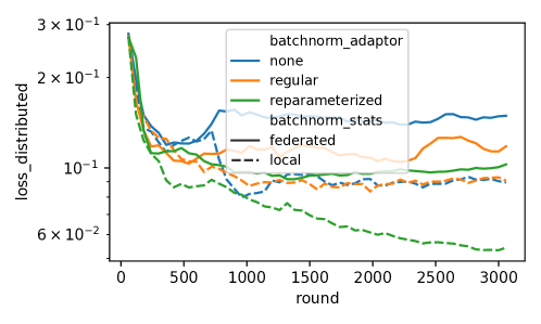
Appendix G Extra Experimental Details
In this section, we show extra experimental details and show missing tables and figures.
G.1 Synthetic Linear
Consider a regression task where we want to learn given , where . We construct two versions of this regression task: one is based on a linear model plus a personalized LoRA, and the other is based on a similar setup on the first layer of a two-layer ReLU net.
For both problems, we sample the parameters of the dataset element-wise from the normal distribution , where is the input dimension of the layer.
The target and the model are such that
| (43) |
where , , , and , and similarly for the trained parameters. The ground-truth model is designed such that the clients share a common structure without making any assumption about the distances of the personal solutions to the solution of FL.
Notice that can make the personal solutions arbitrarily far from , yet they differ in rank only. For example, a simple construction would be and , where is the standard basis vector of the -th coordinate (e.g., ). As for the ground-truth router assignment, we consider a diagonal assignment such that , so clients are in the same cluster for positive integers .
For each client , we take a fixed sample of and of size such that , but , where is the original model size. This is to make it difficult for the model to fit locally due to under-parameterization. Thus, collaboration is important to generalize well, but collaboration with the wrong clients can be detrimental. For this dataset, we chose . The objective for this regression task is the MSE loss .
G.2 Synthetic MLP
Consider a 2-layer ReLU neural net, or multi-layer perceptron (MLP) for short666We write the ReLU function as .
| (44) |
where now , , , and for some hidden dimension , and a diagonal router assignment . We use normal initialization with variance proportional to the input dimension of the layer.
The regression model has the exact same form. However, the hidden dimension is wider, i.e., it is for some integer .
This is mainly because we want to control for the effect of not being able to fit the target model (we set in our experiments). We also have , which is twice as many data points than the linear task as this task is more difficult.
G.3 Ablation and Hyperparameters
| ConvLoRA | CIFAR-10 | CIFAR-100 | |
|---|---|---|---|
| R | LS | ||
| Balanced 2D | 70.2 | 74.1 | 51.7 |
| In Layer | 67.6 | 73.5 | 49.1 |
| Out Layer | 68.5 | 74.0 | 51.9 |
| None | 67.6 | 73.9 | 50.8 |
| Adaptors | Bias | CIFAR-10 | CIFAR-100 | |
|---|---|---|---|---|
| R | LS | |||
| ConvLoRA | ✗ | 69.8 | 72.7 | 45.1 |
| ✓ | 67.6 | 73.4 | 45.8 | |
| LoRA | ✗ | 68.7 | 73.7 | 46.6 |
| ✓ | 67.6 | 73.9 | 50.8 | |
| Both | ✗ | 68.9 | 73.3 | 47.9 |
| ✓ | 70.2 | 74.1 | 51.7 | |
| None | ✗ | 64.6 | 21.9 | 12.1 |
| ✓ | 64.6 | 21.9 | 12.1 | |
Adaptors. We study the effect of removing each of the adaptors introduced in Section 3.2. We chose the CIFAR-10 with both tasks and CIFAR-100 for the ablation study of the LoRAs, ConvLoRAs, and bias adaptors. We show in Figure 8 and Table 5 that the full combination of LoRA, ConvLoRA, and adaptive biases can consistently achieve the top accuracy.
and . In Table 3, we see that choosing to be less than the number of ground-truth clusters can hurt performance. On the other hand, using a significantly larger can hurt performance for smaller , but a larger fixes this by reaching similar accuracies to the case where we know the exact number of ground-truth clusters. We can also see the plots in Figure 9.
ConvLoRA. We compare the different methods for implementing ConvLoRAs as proposed in Section 3.2. We propose to balance the channels and the kernel sizes such that we achieve the most parameter-efficient ConvLoRA, which we refer to as Balanced 2D as it is specific to the two dimensional case. On the other hand, we can balance only the channels and fix the kernel sizes to either the in layer or the out layer. We show in Tables 5 and 10 that the Balanced 2D case is consistently the best option given a fixed . Recall that MNIST and CIFAR-10 have 4 ground-truth clusters, and CIFAR-100 have 10.
G.4 Datasets Meta-data
See Table 6.
G.5 Missing Figures
In this section, we simply show missing figures from our experiments for completeness. In particular, we show plots of the aggregated testing loss per client, which shows how the other methods overfit in comparison to FLoRAL, especially in the low-data regime.