Fourier PINNs: From Strong Boundary Conditions to Adaptive Fourier Bases
Abstract
Interest is rising in Physics-Informed Neural Networks (PINNs) as a mesh-free alternative to traditional numerical solvers for partial differential equations (PDEs). However, PINNs often struggle to learn high-frequency and multi-scale target solutions. To tackle this problem, we first study a strong Boundary Condition (BC) version of PINNs for Dirichlet BCs and observe a consistent decline in relative error compared to the standard PINNs. We then perform a theoretical analysis based on the Fourier transform and convolution theorem. We find that strong BC PINNs can better learn the amplitudes of high-frequency components of the target solutions. However, constructing the architecture for strong BC PINNs is difficult for many BCs and domain geometries. Enlightened by our theoretical analysis, we propose Fourier PINNs — a simple, general, yet powerful method that augments PINNs with pre-specified, dense Fourier bases. Our proposed architecture likewise learns high-frequency components better but places no restrictions on the particular BCs or problem domains. We develop an adaptive learning and basis selection algorithm via alternating neural net basis optimization, Fourier and neural net basis coefficient estimation, and coefficient truncation. This scheme can flexibly identify the significant frequencies while weakening the nominal frequencies to better capture the target solution’s power spectrum. We show the advantage of our approach through a set of systematic experiments.
1 Introduction
Physics-informed neural networks (PINNs) (Raissi et al., 2019) are innovative, mesh-free approaches for solving partial differential equations (PDEs). They offer computationally efficient alternatives to traditional mesh-based numerical methods such as finite elements and finite volumes (Reddy, 2019). The optimization of PINNs involves softly constraining neural networks (NNs) through customized loss functions designed to adhere to the governing equations of physical processes. Researchers have successfully applied PINNs in various domains—for example, they have been used to simulate the radiative transport equation (Mishra & Molinaro, 2021), which is crucial for radio frequency chip and material design (Chen et al., 2020; Liu & Wang, 2019). Further, cardiovascular flow modeling (Kissas et al., 2020) is another application, along with various fluid mechanics problems (Cai et al., 2021), and high-speed aerodynamic flow modeling (Mao et al., 2020), among many others (Raissi et al., 2020; Chen et al., 2020; Jin et al., 2021; Sirignano & Spiliopoulos, 2018; Zhu et al., 2019; Geneva & Zabaras, 2020; Sahli Costabal et al., 2020; Sun et al., 2020; Fang & Zhan, 2019).
Despite these successes, the training of PINNs remains challenging in some instances. Recent studies have analyzed common failure modes of PINNs, particularly when modeling problems that exhibit high-frequency, multi-scale, chaotic, or turbulent behaviors (Wang et al., 2022b; 2020b; 2020a; a), or when the governing PDEs are stiff (Krishnapriyan et al., 2021; Mojgani et al., 2022). Rahaman et al. (2019) attributes the slow convergence to the high-frequency components of the target solution, identifying it as a “spectrum bias” in standard NNs, while learning low-frequency information from data is straightforward. Wang et al. (2020b) confirmed that this bias is also present in the PINN setting. These challenges often arise because applying differential operators over the NN in the residual complicates the loss landscape (Krishnapriyan et al., 2021). From an optimization perspective, Wang et al. (2020a) highlighted that the imbalance in gradient magnitudes between the boundary loss and residual loss (with the latter often being much larger) causes the residual loss to dominate training, leading to a poor fit to the boundary conditions. Wang et al. (2022b) confirmed this conclusion through a neural tangent kernel (NTK) analysis of PINNs with wide networks, finding that the dominant eigenvalues of the residual kernel matrix often result in the training primarily fitting the residual loss.
One class of approaches designed to mitigate the training challenges in PINNs involves setting different weights for the boundary and residual loss terms. For example, Wight & Zhao (2020) suggested incorporating a large multiplier for the boundary loss term to prevent the residual loss from dominating the training process. In contrast, Wang et al. (2020a) proposed a dynamic weighting scheme based on the gradient statistics of the loss terms, and Wang et al. (2022b) developed an adaptive weighting approach based on the eigenvalues of the NTK. Liu & Wang (2021) employed a mini-max optimization to update the loss weights via stochastic ascent, and McClenny & Braga-Neto (2020) used a multiplicative soft attention mask to dynamically re-weight the loss term for each data point and collocation point. To alleviate the spectrum bias in NNs, Tancik et al. (2020) randomly sampled a set of high frequencies from a large-variance Gaussian distribution to construct random Fourier features as input to the NN. Additionally, Wang et al. (2021) used multiple Gaussian variances to sample frequencies for Fourier features, aiming to capture multi-scale solution information within the PINN framework. While effective, the performance of this method is sensitive to the number and scales of the Gaussian variances, which are user-specified hyperparameters that are often difficult to optimize.
Another strategy to improve these challenges is to modify the NN architecture to exactly satisfy the boundary conditions (BCs) (Lu et al., 2021; Lyu et al., 2020; Lagaris et al., 1998; 2000; McFall & Mahan, 2009; Berg & Nyström, 2018; Lagari et al., 2020; Mojgani et al., 2022). We refer to these approaches as “strong BC PINNs”. Despite their effectiveness, these approaches face several limitations. They are usually limited to tasks with relatively simple and well-defined physics, requiring significant craftsmanship and complex implementations even in straightforward problem settings. Consequently, these strategies are less flexible than the original PINN framework, which employs a soft constraint approach for boundary condition satisfaction. Additional complications arise for challenging physical systems governed by invariances or conservation laws, such as energy or momentum conservation, due to often poorly understood and imprecisely defined physical laws. Incorporating these laws effectively into the NN architecture makes extending strong BC PINNs to handle more complex tasks difficult. Further, designing a custom ansatz requires tailoring the NN architecture for each specific boundary condition and domain, which is often impractical for complicated domains. However, when properly designed, these techniques can achieve highly accurate solutions.
In our work, we delve deeper into the training challenges of PINNs for learning high-frequency and multi-scale solutions. We analyze the mechanisms behind the success of strong BC PINNs and explore ways to incorporate these successful strategies into a more general PINN architecture. Our specific contributions are as follows:
-
•
We first examine a strong BC PINN architecture for simple Dirichlet boundary conditions as proposed by Lu et al. (2021). This variant integrates a fixed polynomial boundary function into the NN architecture to exactly satisfy the boundary conditions. While it shows significant improvements over the standard PINN, especially for higher frequency problems, it struggles to predict solutions with frequencies above a certain threshold due to its static nature. To address this limitation, we propose a new strong BC PINN architecture featuring an adaptive parameter optimized during training. This parameter adjusts the boundary function’s sharpness to match the true solution, thereby improving accuracy for higher-frequency solutions compared to the static polynomial variant.
-
•
We conduct a Fourier analysis on both strong BC PINNs compared to the standard PINN. Through the Fourier series convolution theory, we discovered that multiplying the NN by the strong boundary function significantly enhances the learning speed and accuracy of the higher frequency coefficients in the target solution. In contrast, standard PINNs struggle to capture coefficients in the high-frequency domain accurately. This analysis complements and confirms the aforementioned NTK work.
-
•
Inspired by our Fourier analysis, we develop Fourier PINNs. This novel PINN architecture enhances frequency learning within the true solution, comparable to strong BC PINNs, regardless of specific boundary conditions, domain, or underlying physical properties. The Fourier PINN architecture integrates a standard NN with a linear combination of Fourier bases, with frequencies uniformly sampled from an extensive pre-set range. We implement an adaptive learning and basis selection algorithm that alternately optimizes the NN basis parameters and the coefficients of the NN and Fourier bases while pruning insignificant bases. This approach efficiently identifies significant frequencies, supplements those missed by the NN, and improves frequency amplitude estimation (i.e., the basis coefficient) while maintaining computational efficiency. Unlike previous methods, this approach only requires specifying a sufficiently large range and small spacing for the Fourier bases without concern for the actual number and scales of frequencies in the true solution.
-
•
We evaluate Fourier PINNs on several benchmark PDEs characterized by high-frequency and multi-frequency solutions. In all cases, Fourier PINNs consistently achieve low solution errors (e.g., or ). In contrast, standard PINNs invariably fail to achieve comparable accuracy. PINNs with random Fourier features (RFF-PINNs) often fail across various Gaussian variances and scales, indicating high sensitivity to these parameters. Additionally, we test spectral methods, PINNs with large boundary loss weights (Wight & Zhao, 2020), and PINNs with adaptive activation functions (Jagtap et al., 2020). Fourier PINNs consistently outperform all these methods.
The remainder of this paper is structured as follows: Section 2 provides the necessary background and notation, while in Section 4, we present our Fourier analysis of strong BC PINNs and explain the success of the strong boundary ansatz methodology. Our new Fourier PINN architecture and its training routines are described in Section 5. Section 6 details our numerical experiments and findings, including assessments of computational cost and accuracy compared to baseline methods. Finally, Section 7 discusses the results and outlines future research directions.
2 Background
In this section, we first describe the general optimization problems we are addressing with physics-informed neural networks (PINNs) following the formulation presented in Raissi et al. (2019). We then discuss the specifics of strong boundary condition enforcement.
2.1 General Overview of Physics-Informed Neural Networks
The PINN framework uses NNs to estimate solutions to partial differential equations (PDEs). Consider a PDE of the following general form,
| (1) |
where is a linear or non-linear differential operator and represents the unknown solution and is the problem domain in . The general boundary conditions are then,
| (2) |
where is the boundary of the domain and is a general boundary-condition operator.
To solve the PDE, the PINN uses a deep NN, , to approximate the true solution . For clarity in later sections, we follow the convention of Cyr et al. (2020) and define the output of the NN with width as a linear combination of a set of non-linear bases such that,
| (3) |
where each are non-linear activation functions (such as Tanh) acting on the hidden layer outputs. Each for and are the weights and biases in the last layer of the NN and hidden layers, respectively. Therefore, form the set of all network parameters. Then, finding the optimal network parameters involves minimizing the following composite loss function between boundary and residual loss terms,
| (4) |
Here,
| (5) |
is the boundary loss to fit the boundary condition with Lagrange multiplier , and
| (6) |
is the residual loss to fit the equation. We minimize equation 4 by sampling collocation points from the domain and points from the boundary of the domain , and iteratively modifying the network parameters through gradient descent.
2.2 Strong Boundary Condition PINNs
Equation 5 can approximately enforce various types of boundary conditions, including Dirichlet, Neumann, Robin, and periodic. However, prior analysis by Wang et al. (2020a; 2022b) suggests that the instability in training PINNs likely arises from the competition between the weakly enforced boundary loss (5) and the residual loss (6) terms during optimization. This competition likely occurs because both loss terms are minimized simultaneously during training. However, the optimization algorithm tends to prioritize the minimization of the residual loss, as it typically dominates the gradient of the combined loss function. Consequently, this can lead to a scenario where the residual loss converges effectively but at the expense of the boundary loss, which remains inadequately optimized. As a result, the boundary conditions may not be satisfied, leading to poor model performance on new, unseen data or data at the domain’s boundaries.
One solution to mitigate the competition between the loss terms is to design a surrogate model that inherently satisfies the boundary conditions. This approach typically works by modifying the network architecture to satisfy the boundary conditions exactly, thus eliminating the need for a boundary enforcement loss term and further reducing the computational cost. This method of exact imposition of boundary conditions has become a standard approach in the PINN literature and is especially prevalent for Dirichlet and periodic boundary conditions (Lu et al., 2021; Yu et al., 2022; Wang et al., 2024).
This work primarily focuses on Dirichlet boundary conditions to simplify the analysis and implementations while addressing a significant and common scenario in physical systems. Dirichlet boundary conditions provide a clear and straightforward framework to demonstrate the effectiveness of the surrogate model approach, as they require the solution to take specific values at the boundaries, which is relatively easy to enforce exactly on simplified domains. To illustrate, we consider the 1D Dirichlet boundary condition defined as,
| (7) |
For this case, the surrogate model is typically defined as,
| (8) |
such that is the solution function, is the provided boundary function, is the output of the neural network, and is a composite distance function that zeroes out on the boundaries, ensuring the boundary conditions are met without explicit penalty terms. By construction, , and thus the boundary condition in equation 7 is strictly and automatically satisfied. To estimate the parameters of , we only need to minimize the residual loss . Most PINN surrogate model designs rely on distance functions based on the theory of R-functions (Sukumar & Srivastava, 2022), which are smooth mathematical functions that encode Boolean logic and facilitate the combination of simple shapes to form complex geometries (Rvachev & Sheiko, 1995). Some meshfree Galerkin methods have utilized the capability of R-functions to enforce boundary conditions smoothly and exactly to enhance the precision and robustness of numerical simulations for solving boundary-value problems (Shapiro & Tsukanov, 1999; Akin, 2014; Tsukanov & Posireddy, 2011).
In this work, we compare the standard PINN to two strong BC PINNs using different distance functions to enforce Dirichlet boundary conditions exactly. The first distance function we consider is the polynomial distance function proposed in (Lu et al., 2021), defined as,
| (9) |
This function satisfies the boundary conditions by zeroing out at the endpoints and . While Lu et al. (2021) demonstrates promising results using this formulation, the polynomial distance function remains static throughout the training process. The absence of adaptability limits the model’s performance across different problems and domains, whereas introducing adaptability would allow the model to adjust to the varying complexities within the solution space.
To address this limitation, we propose an adaptive distance function to introduce flexibility in enforcing the boundary conditions, which we define as:
| (10) |
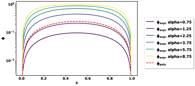
where is a parameter that can be pre-set or optimized during training. The exponential form of equation 10 allows the function to adjust dynamically to better conform to the unique characteristics of the problem domain, thus enhancing the enforcement of boundary conditions across different scenarios and potentially leading to more accurate and efficient training outcomes.
Figure 1 illustrates the behavior of the polynomial distance function to the exponential distance function with various values of . As varies, adjusts its shape, showcasing its ability to conform to different problem domains and complexities. We expect this dynamic adaptability to enhance the model’s performance by more precisely enforcing boundary conditions across diverse scenarios. We affirm this through a numerical example in the next section.
3 Boundary Condition Pathologies in PINNs
Recent works have employed strong boundary enforcement strategies (Lu et al., 2021; Yu et al., 2022) but offer few insights into the specific surrogate model design process. The design and implementation of the surrogate models are often ad-hoc, with no systematic approach to their architectural design. This complicates their application and limits their effectiveness across boundary conditions and physical problems, especially when dealing with complex physics and domains. Moreover, the standard PINNs frequently encounter difficulties with high-frequency and multi-scale solutions, leading to inaccurate predictions (Wang et al., 2020b). We show that while the strong BC PINN model improves solution quality for problems with higher frequency compared to the standard PINN, the solution quality nevertheless degrades with larger frequencies. In the following, we empirically demonstrate how the standard PINN solution quality degrades as the actual frequency of the solution increases in both a linear 1D Poisson problem and a non-linear 1D steady-state Allen-Cahn problem. Specifically, we consider the fabricated solution for a range of frequencies and . Therefore, by varying , we can examine the performance of the standard PINNs compared to the strong BC PINNs when the solution includes different frequency information.
Specifically, we examine the 1D Poisson equation given by,
| (11) | ||||
| (12) |
and derive the forcing function from the fabricated solution which gives . We also consider the 1D Allen-Cahn equation defined as,
| (13) | ||||
| (14) |
which gives the forcing function . Both are subject to the Dirichlet condition in equation 7 where and . We test these problems using a standard PINN, which explicitly incorporates the weakly enforced boundary loss and residual loss terms. We compare these results to two strong BC PINNs employing different distance functions (8) and show that this method exhibits slower solution degradation with increased frequency. We used the same NN architecture for the strong BC PINN and the standard PINN, including two hidden layers, neurons per layer, and Tanh activation. Both methods used the same 10K collocation points randomly sampled from the domain. We report the averaged results for each method from five random trials.

Figure 2 shows that both of the strong BC PINNs given by equation 9 and equation 10 push the surrogate model to inhibit the high-frequency components resulting in higher accuracy solutions, however, once the frequency surpasses a certain threshold, the static polynomial distance function fails to provide any additional benefit. Figure 2 shows that the strong BC PINN () given by equation 10 obtains higher accuracy solutions than both the standard PINN and the strong BC PINN (). However, it similarly hits a threshold where the benefits of the strong boundary enforcement diminish, albeit at a much higher frequency than the strong BC PINN ().
4 Fourier Analysis of Strong BC PINNs
In this section, we explain why the strong BC PINNs outperform standard PINNs using Fourier analysis. Both NNs and PINNs often exhibit spectral bias, quickly capturing low-frequency information but struggling with high-frequency components (Basri et al., 2020; Rahaman et al., 2019; Xu et al., 2019; Wang et al., 2021). This bias means that while NNs can quickly grasp general patterns (low frequencies), they struggle with capturing finer details (high frequencies), leading to potential inaccuracies in the solution. The frequency spectrum of a PINN showing spectral bias would show large coefficients at low frequencies, indicating that the NN has effectively captured the low-frequency components of the target solution. In contrast, the coefficients for high-frequency components would decay slowly and exhibit heavy tails, indicating that the network is not effectively filtering out the high-frequency noise or inaccuracies. These tails suggest that the high-frequency components, even though not dominant, still have significant amplitudes. Overall, the frequency spectrum would highlight a pronounced low-frequency peak with a gradual and insufficient reduction in the magnitude of higher frequencies, reflecting the network’s difficulty in learning and accurately representing the high-frequency aspects of the solution.
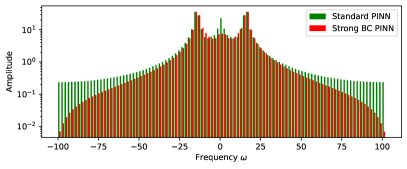
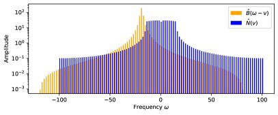
Figure 3 shows the frequency spectrum from the discrete Fourier transform of a standard PINN trained to solve the 1D Poisson problem defined in equation 12 with the true solution for , where the solution frequency is . Although the standard PINN identifies the target frequency seen by the large coefficient at , it exhibits large coefficients for higher frequencies, leading to heavy tails and reduced accuracy. In contrast, the frequency spectrum of the strong BC PINN (Figure 3) demonstrates that it not only captures the target frequency as accurately as the standard PINN, but its higher frequency coefficients decay much faster. This rapid decay weakens or excludes the influence of unnecessary high frequencies, resulting in significantly improved accuracy. In simpler terms, while both networks can identify the main pattern in the data (the target frequency), the strong BC PINN is better at ignoring unnecessary noise (high-frequency components) which leads to a more accurate overall solution.
To analyze why the distance function () after multiplied to the NN in equation 8 can help obtain better coefficients for high frequencies, we first represent the general boundary function as an infinite Fourier series,
| (15) |
where indicates the imaginary part and are integers. We first analyze the polynomial distance function by substituting equation 9 for in equation 15 giving,
| (16) |
Similarly, to compare against our proposed adaptive distance function, we substitute in equation 10 for in equation 15 and obtain,
| (17) |
Here, we expand the boundary functions to be periodic (i.e., duplicating its definition in to other intervals) and the period is . We can now obtain the Fourier transforms of each by evaluating,
| (18) |
where is the Dirac delta function and is the continuous frequency. Specifically, each represents the Fourier transform of , meaning where denotes the inverse Fourier transform.
Since , the amplitude of the frequencies of decay quadratically fast with the increase of the absolute frequency value. This rapid decay is beneficial for denoising as it effectively suppresses high-frequencies leading to smoother approximations. However, it may result in the loss of fine details, especially if important signal components are present at higher frequencies. Alternatively, , indicating that the frequency amplitudes follow Lorentzian decay controlled by the decay rate . Lorentzian decay is less aggressive in reducing high-frequency components, which helps preserve fine details and sharp transitions in the signal. This flexibility is useful in tuning the decay based on signal characteristics, however, the slower decay rate may lead to less effective noise suppression.
We can now look at the frequency spectrum of the full surrogate model in equation 8. We use the convolution theorem (McGillem & Cooper, 1991) to obtain
| (19) |
where denotes convolution, and is the Fourier transform of the NN. Suppose , we know that is obtained by first reflecting about the y-axis, and then shifting the frequency left along the spectrum. Then, we integrate weighted by . The larger the frequency , the more is moved left to obtain resulting in a stronger weighting of the high-frequency components during integration. Since the frequency coefficients of decay quadratically fast (), the larger the portion of the tail is used, and the smaller the integration result. Specifically, with , the corresponding amplitude of decrease fast when increases111The same conclusion applies when we consider .. See Figure 3 for an illustration. Thereby, during the course of training, the boundary function pushes the surrogate model in equation 8 to weaken irrelevant high-frequency components to reduce large tails and to better capture the frequency spectrum.
5 Fourier PINNs
Our Fourier analysis in the previous section revealed that the standard PINNs inefficiently capture the true amplitude of frequencies in the power spectrum of their predicted solutions. Specifically, the analysis showed that although standard PINNs could identify the true solution frequency, they failed to prune large and noisy frequencies, as indicated by the large amplitudes assigned at the tail end of the power spectrum in Figure 3. While the strong BC PINNs address this issue by multiplying the NN with a boundary function—which helps decay high-frequency amplitudes faster—their overall benefit remains limited. As shown in Figure 2, performance degrades as increases, indicating the boundary function’s inability to learn ultra-high frequency solutions. Additionally, the strong BC PINNs are restricted to specific boundary conditions, such as Dirichlet conditions in equation 7, limiting their applicability.
5.1 Fourier PINNs
To overcome these challenges, we introduce Fourier PINNs, a novel PINN architecture. Fourier PINNs seamlessly handle diverse boundary conditions, like the standard PINNs, while emphasizing the true solution frequencies during training—akin to the strong BC PINNs. Specifically, in order to flexibly yet comprehensively capture the frequency spectrum, we first introduce a set of dense frequency candidates, , evenly sampled from the range . From this set of frequency candidates, we define a set of trainable Fourier bases as,
| (20) |
The Fourier PINN architecture additively combines the outputs of both the NN from equation 3 and the Fourier bases from equation 20 to generate the augmented prediction . Specifically, the full output of Fourier PINNs is,
| (21) |
We define as the set of all basis coefficients, and form the set of all trainable network parameters.
While we present our method in the one dimensional input case, it is straightforward to extend to multiple dimensions. Consider the two dimensional input for an example. We use the same set of frequencies to construct Fourier bases for each input. Specifically, we construct
and
Then we apply the cross-product of and to obtain the tensor-product Fourier bases for . The surrogate model is given by,
| (22) |
where denotes the vectorization, and are the coefficients of the Fourier bases. Note that the tensor-product of bases grows exponentially with the problem dimension, quickly becoming computationally intractable. One potential solution is to generate more sparse Fourier bases, such as total-degree or hyperbolic cross bases. Another option is to re-organize the coefficients into a tensor or matrix and introduce a low-rank decomposition structure to parameterize to save computational cost (Novikov et al., 2015). These explorations are left for future work.
5.2 Adaptive Basis Selection Training Algorithm
Given that the ground-truth solution likely contains significantly fewer frequencies than the augmented candidate bases (), and our previous analysis showed that models often struggle to prioritize learning necessary frequencies, we developed an adaptive learning and basis selection algorithm. This algorithm flexibly identifies meaningful frequencies while pruning the inconsequential ones—allowing the model to focus on learning and improving the bases that significantly contribute to the solution by inhibiting the learning of unnecessary (and likely noisy) frequencies.
To aid in identifying the significant frequencies, we add an regularization term to the basis parameters . This additional regularization penalizes large coefficients for the basis functions, thereby promoting sparsity and encouraging the model to focus on learning the most significant frequencies. The full loss function we use is similar to PINNs (see equation 4), but with the addition of the regularization term. Specifically, the loss function is,
| (23) |
where represents the regularization of and is the regularization strength defined by the user prior to initiating training. This regularization term helps prune or inhibit unnecessary frequencies, allowing the model to focus more on learning and improving the bases that significantly contribute to the solution.
Our adaptive basis selection algorithm optimizes the regularized loss function in equation 23 by building upon the hybrid least squares gradient descent method proposed by Cyr et al. (2020). Cyr et al. (2020) formulates the output of a neural network as a linear combination of non-linear basis functions, as shown in equation 3. Their algorithm alternates between optimizing the hidden weights () via gradient descent and the final layer coefficients () through the least squares problem of the form,
| (24) |
such that for the data points , for , and is some linear operator. equation 24 extends to problems with multiple operators, such as those defined by equation 1 and equation 2 when and are linear operators.
Representing the output of Fourier PINNs in equation 20 as a linear combination of both adaptive bases (i.e., the hidden layers of the NN) and an augmented Fourier series ensures our model’s compatibility with the general approach of the alternating least squares and gradient descent optimization. While Cyr et al. (2020) hold the coefficients c constant while optimizing the bases through gradient descent, we alternatively choose to jointly optimize both the basis coefficients and the adaptive bases during the gradient descent step. During the least squares step, we solve a similar problem to equation 24 modified to suit the Fourier PINN architecture. Specifically, we solve the least squares problem of the form,
| (25) |
such that for the data points , and
| (26) |
We define equation 25 for one operator , but the method extends to multiple operators. Additionally, we extend our least-squares method to non-linear operators, unlike many works that focus only on linear cases.
Specifically, when the operator is nonlinear, the coefficient updates of require more careful consideration. We consider non-linear operators , that can be decomposed into linear and nonlinear parts such as,
| (27) |
where is a linear operator and is the nonlinear part. For illustration, consider the Allen-Cahn problem define by equation 14. We have and , and solve equation 25 such that for the data points . Here, are the Fourier PINN’s evaluations with the current on the set of points, and
| (28) |
In this case, since b is determined from the current but fixed as a constant in the least squares estimation, the update of is in essense a type of fixed point iteration. When does not include any linear operator (which might be rare), we can use any continues optimization algorithm, e.g., L-BFGS, to update .
We integrate a custom basis pruning routine into the optimization algorithm to eliminate insignificant bases and refine model training. Our modified loss function defined in equation 23 enhances this hybrid optimization algorithm with an regularization term to identify and prioritize significant frequencies. Algorithm 1 outlines our adaptive learning routine. The algorithm begins with a joint optimization of and to provide a warm start to the model parameters. Next, we fix while alternating between solving for the coefficients using the least squares method and truncating bases with coefficients below a predefined threshold. Specifically, bases corresponding to are removed along with . After completing the alternating solve and truncate steps for a set number of iterations, the algorithm jointly optimizes all remaining parameters and bases using the Adam optimization algorithm. We repeat this routine for a fixed number of iterations, followed by L-BFGS optimization until the final convergence.
6 Experiments
In this section, we present a series of tests comparing our methods against a range of PDE problems. These include the 1D and 2D Poisson equations, which are canonical linear elliptic PDE problems, and the 1D and 2D (steady-state) Allen-Cahn equations, which are non-linear elliptic PDEs demonstrating the effect of adding a non-linear reaction term. Additionally, we analyze the 1D (one-way) Wave equation to observe the impact of incorporating a first time derivative. We first describe the baseline methods we compare against Fourier PINNs, then list our experimental details. Finally, we provide a detailed discussion after presenting the results comparing each baseline on the example problems.
6.1 Baselines
We benchmarked against the following state-of-the-art PINN models for solving high-frequency and/or multi-scale solutions:
-
(1)
(PINN) standard PINNs as formulated in (Raissi et al., 2017);
- (2)
-
(3)
(W-PINN) Weighted PINNs that down-weight the residual loss term to reduce its dominance and to better fit the boundary loss Wang et al. (2022b);
-
(4)
(A-PINN) Adaptive PINNs with parameterized activation functions to increase the NN capacity and to be less prone to gradient vanishing and exploding Jagtap et al. (2020); and
-
(5)
(Spectral) standard Spectral Methods (Boyd, 2001), which approximate solutions using a linear combination of Fourier bases, and estimates the basis coefficients via least mean squares222Throughout the experiments, we used the same set of Fourier bases for the spectral method and our method..
We do not test against the conceptually similar Fourier Neural Operators Li et al. (2020) as they are designed to solve the inverse problem, thus requiring a data loss term. Our method is designed to solve forward problems and requires no training data within the domain.
| Number | Scales |
|---|---|
| 1 | , , , |
| 2 | , , , , |
| 3 | , , , , |
| 5 |
6.2 Hyperparameters and experimental details
All code is implemented in PyTorch333Code will be made available upon acceptance. For all the NN based methods, we used two hidden layers, with neurons per layer and the Tanh activation function. We ran every method for five random trials, and report the five number summaries for each test in boxplot form. For PINN, W-PINN, A-PINN and RFF-PINN, we first ran K iterations of the Adam optimizer (Kingma & Ba, 2014) with a learning rate of , and then L-BFGS optimizer (Liu & Nocedal, 1989) until convergence (with the tolerance set to ). In Fourier PINNs, we specified the range of frequency candidates in the Fourier bases by setting a maximum frequency and including all equally spaced frequencies in the set . In Algorithm 1, we set , the number of iterations to 1K, the inner iteration number to 5, the truncation threshold to , and the outer iteration number to 40. RFF-PINNs require specifying both the number and scales of the Gaussian variances used to construct the random features. To comprehensively evaluate the effect of both hyperparameters, we tested RFF-PINNs with 20 different settings. We used one, two, three and five scales, and set the variances to common values suggested in (Wang et al., 2021), combined with randomly sampled ones. The exact sets of chosen scales are listed in Table 1. For W-PINN, we varied the weight of the residual loss from , and for A-PINN, we introduced a learned parameter for the activation function in each layer and update these parameters jointly.
6.3 1D Numerical Experiments
In this section, we demonstrate the performance of our methods compared to each baseline on 1D problems including the 1D Poisson, 1D steady-state Allen-Cahn, and 1D One-Way Wave equation. We first tested a set of 1D Poisson problems (see equation 12) with the following ground-truth solutions,
| (29) | ||||
| (30) | ||||
| (31) |
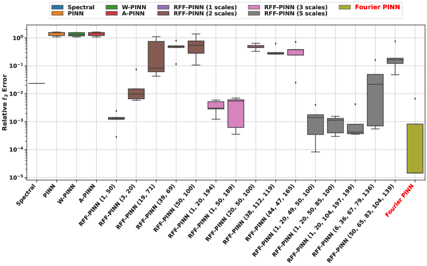
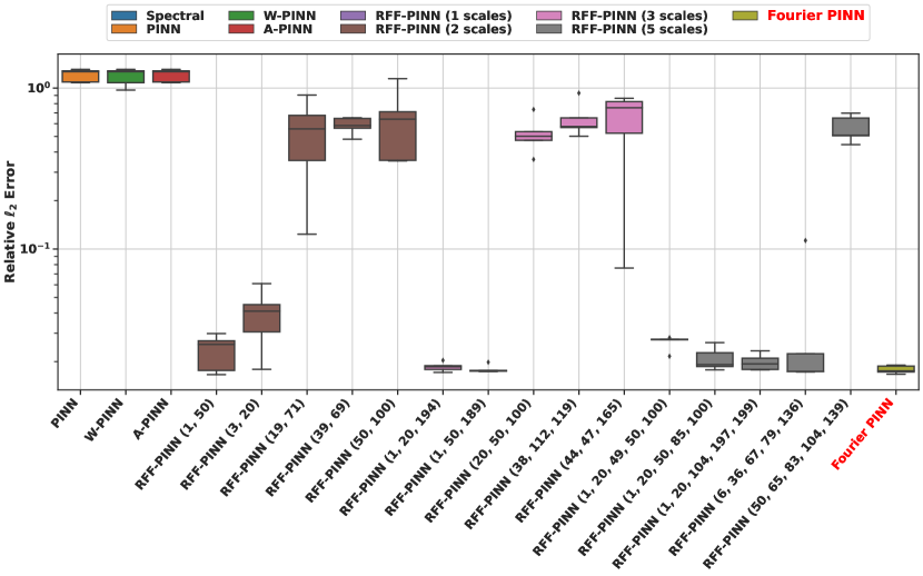
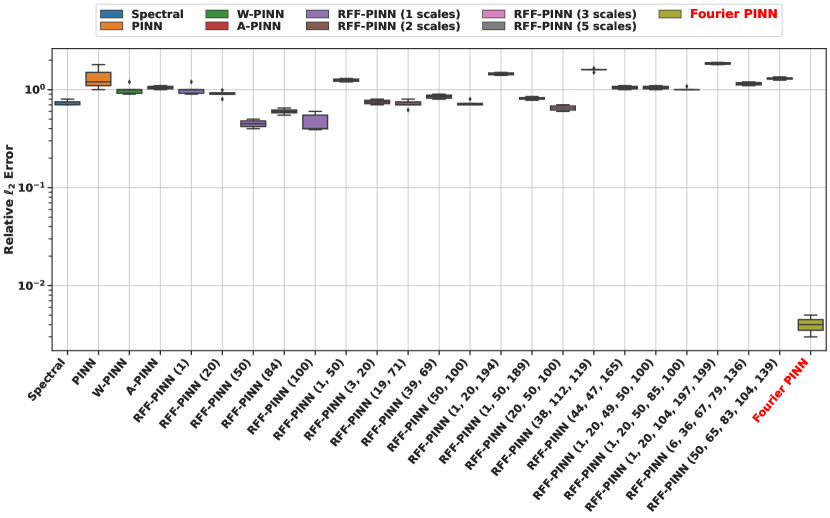
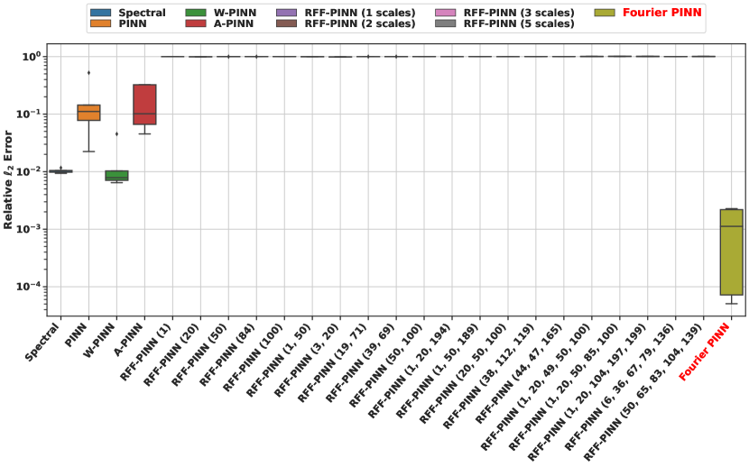
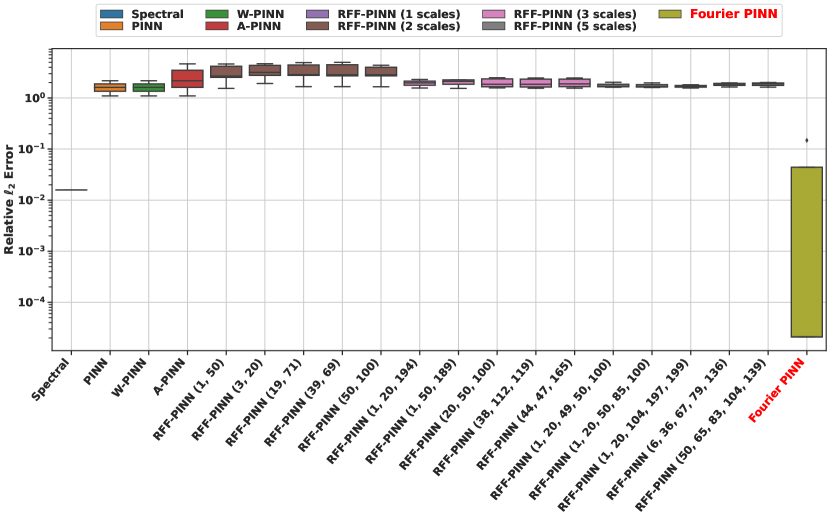
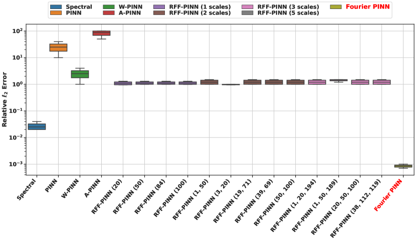
The boundary conditions are derived from the true solution. We visualize the relative errors for each baseline method on these problems in Figures 4, 5, and 6 respectively. For Fourier PINNs, we set and for problems equation 29 and equation 30, then simply set for the remaining tests. Then, we examined the 1D steady-state Allen-Cahn equation of the form 14 with the same true manufactured solutions as for the 1D Poisson problem and report the results in Figures 7, 8, and 9. The final 1D problem we tested is the 1D One-Way Wave equation of the form,
| (32) | |||
with a true solution of,
| (33) |
The results are reported in Figure 10.
6.4 2D Numerical Experiments
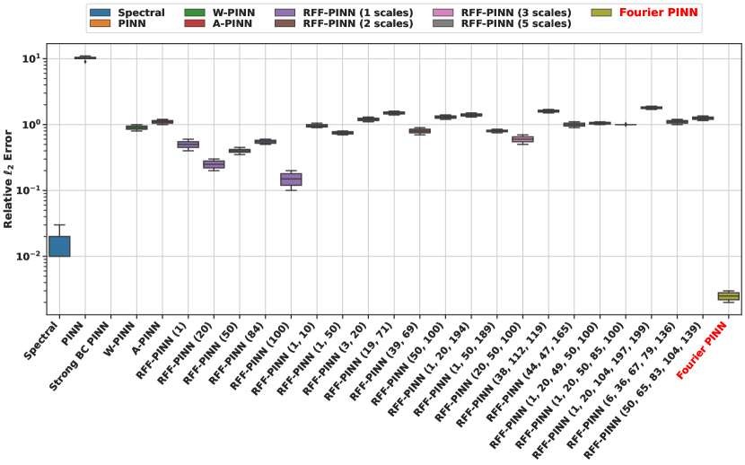
In this section, we demonstrate the performance of our methods compared to each baseline on 2D problems, including the 2D Poisson and 2D steady-state Allen-Cahn equations. We first tested on the 2D Poisson problem given by,
| (34) |
with the following ground-truth manfactured solutions,
| (35) | ||||
| (36) |
We visualize the relative errors for each baseline method on these examples in Figures 11 and 12 respectively. We next tested on the 2D steady-state Allen-Cahn problem which is given by.
| (38) |
with the ground-truth solution,
| (39) |
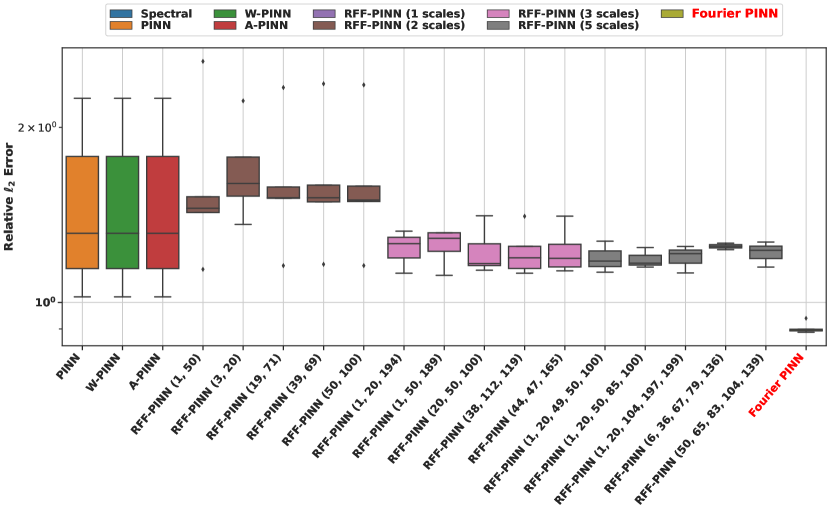
and we report the results in Figure 13. Note that in these tests, the RFF-PINN method failed and resulted in large relative errors for all the single-scale settings, therefore we did not report these results.
6.5 Discussion
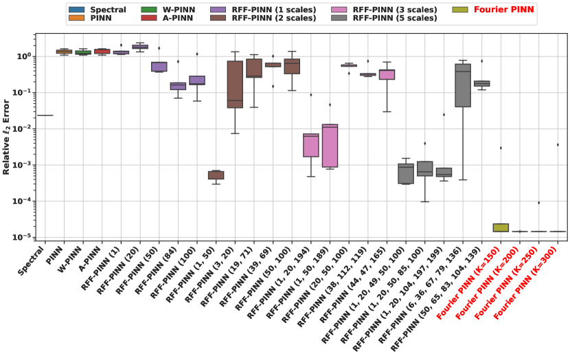
We can see that in all examples for both the 1D and 2D problems, the standard PINN, W-PINN, and A-PINN failed to obtain reasonable solutions, with large relative errors for all cases (e.g.,). This implies that these methods are unable to capture high-frequency signals. Additionally, RFF-PINN can achieve small relative errors with particular scale settings; however, for most settings (60-70% of the 20 total RFF-PINN settings listed in Table 1), RFF-PINN failed with large solution errors. These results show that the success of RFF-PINN is very sensitive to the choice of number and scales, and there is no apparent correspondence between scale settings and problem solutions. For example, for the single-scale true solution (see Figure 4), the successful cases of RFF-PINN include two, three or even five scale settings, e.g.,(1, 20, 194), yet it failed with all the single-scale settings. The spectral method also failed to obtain good solutions, implying that only estimating a linear combination of Fourier bases are not sufficient. As a comparison, Fourier PINNs achieves reasonable solution accuracy in all the cases, with relative errors between and . Our method is also robust to the choice of the frequency range . As long as is large enough, our method nearly always selected the target frequency, and returned similar solution accuracy. Note that, to focus on the evaluation of the key idea, Fourier PINNs did not employ any loss term re-weighting schemes to further improve the accuracy, such as the NTK re-weighting used in RFF-PINN or mini-max updates. However, it would be straightforward to integrate these methods into the proposed algorithmic framework.
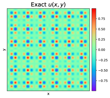
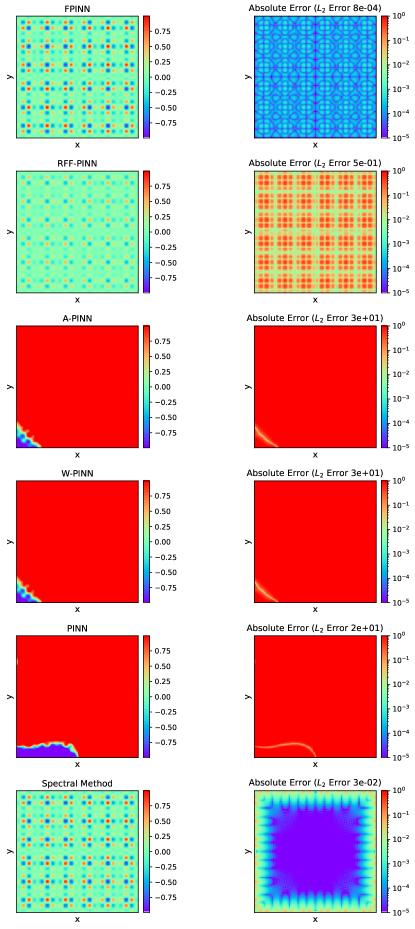
We finally visualize the solution of each method in solving a 2D Poisson equation (see Figure 12) to visualize the point-wise errors for each method within the two dimensional domain. The ground-truth solution is given in Figure 14 and the solution obtained by each method is shown in Figure 15. Note that for W-PINN and RFF-PINN, we report the result with the smallest relative error. While the spectral method also obtains good results, the point wise error biases much on the regions that are close to the boundary and the relative error is two orders of magnitude larger than Fourier PINN’s. RFF-PINN (with the best number and scale choice) can roughy capture the solution structure, but the accuracy is far worse than Fourier PINNs and the spectral method. For example, in Figure 12, RFF-PINN nearly failed with every choice of the number and scale set. We can see that overall, Fourier PINNs best recovers the original solution.
7 Conclusion
We have presented Fourier PINNs, a novel PINN extension to capture high-frequency and multi-scale solution information. Our adaptive basis learning and selection algorithm can automatically identify target frequencies and truncate useless ones, without the need for tuning the number and scales. Currently, we assume the spacing (granularity) of the candidate frequencies is fine-grained enough, which can be overly optimistic. In the future, we plan to develop adaptive spacing approaches to capture this granularity.
Acknowledgments
We acknowledge the use of large language models (LLMs) for manuscript editing.
References
- Akin (2014) John E Akin. Finite elements for analysis and design: computational mathematics and applications series. Elsevier, 2014.
- Basri et al. (2020) Ronen Basri, Meirav Galun, Amnon Geifman, David Jacobs, Yoni Kasten, and Shira Kritchman. Frequency bias in neural networks for input of non-uniform density. In International Conference on Machine Learning, pp. 685–694. PMLR, 2020.
- Berg & Nyström (2018) Jens Berg and Kaj Nyström. A unified deep artificial neural network approach to partial differential equations in complex geometries. Neurocomputing, 317:28–41, 2018.
- Boyd (2001) John P Boyd. Chebyshev and Fourier spectral methods. Courier Corporation, 2001.
- Cai et al. (2021) Shengze Cai, Zhiping Mao, Zhicheng Wang, Minglang Yin, and George Em Karniadakis. Physics-informed neural networks (PINNs) for fluid mechanics: a review. Acta Mechanica Sinica, 37(12):1727–1738, December 2021. ISSN 1614-3116. doi: 10.1007/s10409-021-01148-1. URL https://doi.org/10.1007/s10409-021-01148-1.
- Chen et al. (2020) Yuyao Chen, Lu Lu, George Em Karniadakis, and Luca Dal Negro. Physics-informed neural networks for inverse problems in nano-optics and metamaterials. Optics express, 28(8):11618–11633, 2020.
- Cyr et al. (2020) Eric C. Cyr, Mamikon A. Gulian, Ravi G. Patel, Mauro Perego, and Nathaniel A. Trask. Robust Training and Initialization of Deep Neural Networks: An Adaptive Basis Viewpoint. In Proceedings of The First Mathematical and Scientific Machine Learning Conference, pp. 512–536. PMLR, August 2020. URL https://proceedings.mlr.press/v107/cyr20a.html. ISSN: 2640-3498.
- Fang & Zhan (2019) Zhiwei Fang and Justin Zhan. Deep physical informed neural networks for metamaterial design. IEEE Access, 8:24506–24513, 2019.
- Geneva & Zabaras (2020) Nicholas Geneva and Nicholas Zabaras. Modeling the dynamics of pde systems with physics-constrained deep auto-regressive networks. Journal of Computational Physics, 403:109056, 2020.
- Jagtap et al. (2020) Ameya D Jagtap, Kenji Kawaguchi, and George Em Karniadakis. Adaptive activation functions accelerate convergence in deep and physics-informed neural networks. Journal of Computational Physics, 404:109136, 2020.
- Jin et al. (2021) Xiaowei Jin, Shengze Cai, Hui Li, and George Em Karniadakis. Nsfnets (navier-stokes flow nets): Physics-informed neural networks for the incompressible navier-stokes equations. Journal of Computational Physics, 426:109951, 2021.
- Kingma & Ba (2014) Diederik P Kingma and Jimmy Ba. Adam: A method for stochastic optimization. arXiv preprint arXiv:1412.6980, 2014.
- Kissas et al. (2020) Georgios Kissas, Yibo Yang, Eileen Hwuang, Walter R. Witschey, John A. Detre, and Paris Perdikaris. Machine learning in cardiovascular flows modeling: Predicting arterial blood pressure from non-invasive 4d flow mri data using physics-informed neural networks. Computer Methods in Applied Mechanics and Engineering, 358:112623, 2020. ISSN 0045-7825. doi: https://doi.org/10.1016/j.cma.2019.112623. URL https://www.sciencedirect.com/science/article/pii/S0045782519305055.
- Krishnapriyan et al. (2021) Aditi Krishnapriyan, Amir Gholami, Shandian Zhe, Robert Kirby, and Michael W Mahoney. Characterizing possible failure modes in physics-informed neural networks. Advances in Neural Information Processing Systems, 34:26548–26560, 2021.
- Lagari et al. (2020) Pola Lydia Lagari, Lefteri H Tsoukalas, Salar Safarkhani, and Isaac E Lagaris. Systematic construction of neural forms for solving partial differential equations inside rectangular domains, subject to initial, boundary and interface conditions. International Journal on Artificial Intelligence Tools, 29(05):2050009, 2020.
- Lagaris et al. (1998) Isaac E Lagaris, Aristidis Likas, and Dimitrios I Fotiadis. Artificial neural networks for solving ordinary and partial differential equations. IEEE transactions on neural networks, 9(5):987–1000, 1998.
- Lagaris et al. (2000) Isaac E Lagaris, Aristidis C Likas, and Dimitris G Papageorgiou. Neural-network methods for boundary value problems with irregular boundaries. IEEE Transactions on Neural Networks, 11(5):1041–1049, 2000.
- Li et al. (2020) Zongyi Li, Nikola Kovachki, Kamyar Azizzadenesheli, Burigede Liu, Kaushik Bhattacharya, Andrew Stuart, and Anima Anandkumar. Fourier neural operator for parametric partial differential equations. arXiv preprint arXiv:2010.08895, 2020.
- Liu & Wang (2019) Dehao Liu and Yan Wang. Multi-fidelity physics-constrained neural network and its application in materials modeling. Journal of Mechanical Design, 141(12), 2019.
- Liu & Wang (2021) Dehao Liu and Yan Wang. A dual-dimer method for training physics-constrained neural networks with minimax architecture. Neural Networks, 136:112–125, 2021.
- Liu & Nocedal (1989) Dong C Liu and Jorge Nocedal. On the limited memory bfgs method for large scale optimization. Mathematical programming, 45(1-3):503–528, 1989.
- Lu et al. (2021) Lu Lu, Raphael Pestourie, Wenjie Yao, Zhicheng Wang, Francesc Verdugo, and Steven G Johnson. Physics-informed neural networks with hard constraints for inverse design. SIAM Journal on Scientific Computing, 43(6):B1105–B1132, 2021.
- Lyu et al. (2020) Liyao Lyu, Keke Wu, Rui Du, and Jingrun Chen. Enforcing exact boundary and initial conditions in the deep mixed residual method. arXiv preprint arXiv:2008.01491, 2020.
- Mao et al. (2020) Zhiping Mao, Ameya D. Jagtap, and George Em Karniadakis. Physics-informed neural networks for high-speed flows. Computer Methods in Applied Mechanics and Engineering, 360:112789, 2020. ISSN 0045-7825. doi: https://doi.org/10.1016/j.cma.2019.112789. URL https://www.sciencedirect.com/science/article/pii/S0045782519306814.
- McClenny & Braga-Neto (2020) Levi McClenny and Ulisses Braga-Neto. Self-adaptive physics-informed neural networks using a soft attention mechanism. arXiv preprint arXiv:2009.04544, 2020.
- McFall & Mahan (2009) Kevin Stanley McFall and James Robert Mahan. Artificial neural network method for solution of boundary value problems with exact satisfaction of arbitrary boundary conditions. IEEE Transactions on Neural Networks, 20(8):1221–1233, 2009.
- McGillem & Cooper (1991) Clare D McGillem and George R Cooper. Continuous and discrete signal and system analysis. Harcourt School, 1991.
- Mishra & Molinaro (2021) Siddhartha Mishra and Roberto Molinaro. Physics informed neural networks for simulating radiative transfer. Journal of Quantitative Spectroscopy and Radiative Transfer, 270:107705, 2021.
- Mojgani et al. (2022) Rambod Mojgani, Maciej Balajewicz, and Pedram Hassanzadeh. Lagrangian pinns: A causality-conforming solution to failure modes of physics-informed neural networks. arXiv preprint arXiv:2205.02902, 2022.
- Novikov et al. (2015) Alexander Novikov, Dmitrii Podoprikhin, Anton Osokin, and Dmitry P Vetrov. Tensorizing neural networks. Advances in neural information processing systems, 28, 2015.
- Rahaman et al. (2019) Nasim Rahaman, Aristide Baratin, Devansh Arpit, Felix Draxler, Min Lin, Fred Hamprecht, Yoshua Bengio, and Aaron Courville. On the spectral bias of neural networks. In International Conference on Machine Learning, pp. 5301–5310. PMLR, 2019.
- Raissi et al. (2017) Maziar Raissi, Paris Perdikaris, and George Em Karniadakis. Physics informed deep learning (part i): Data-driven solutions of nonlinear partial differential equations. arXiv preprint arXiv:1711.10561, 2017.
- Raissi et al. (2019) Maziar Raissi, Paris Perdikaris, and George E Karniadakis. Physics-informed neural networks: A deep learning framework for solving forward and inverse problems involving nonlinear partial differential equations. Journal of Computational Physics, 378:686–707, 2019.
- Raissi et al. (2020) Maziar Raissi, Alireza Yazdani, and George Em Karniadakis. Hidden fluid mechanics: Learning velocity and pressure fields from flow visualizations. Science, 367(6481):1026–1030, 2020.
- Reddy (2019) Junuthula Narasimha Reddy. Introduction to the finite element method. McGraw-Hill Education, 2019.
- Rvachev & Sheiko (1995) Vladimir L Rvachev and Tatyana I Sheiko. R-functions in boundary value problems in mechanics. 1995.
- Sahli Costabal et al. (2020) Francisco Sahli Costabal, Yibo Yang, Paris Perdikaris, Daniel E Hurtado, and Ellen Kuhl. Physics-informed neural networks for cardiac activation mapping. Frontiers in Physics, 8:42, 2020.
- Shapiro & Tsukanov (1999) Vadim Shapiro and Igor Tsukanov. Meshfree simulation of deforming domains. Computer-Aided Design, 31(7):459–471, 1999.
- Sirignano & Spiliopoulos (2018) Justin Sirignano and Konstantinos Spiliopoulos. Dgm: A deep learning algorithm for solving partial differential equations. Journal of computational physics, 375:1339–1364, 2018.
- Sukumar & Srivastava (2022) N. Sukumar and Ankit Srivastava. Exact imposition of boundary conditions with distance functions in physics-informed deep neural networks. Computer Methods in Applied Mechanics and Engineering, 389:114333, 2022. ISSN 0045-7825. doi: 10.1016/j.cma.2021.114333. URL https://www.sciencedirect.com/science/article/pii/S0045782521006186.
- Sun et al. (2020) Luning Sun, Han Gao, Shaowu Pan, and Jian-Xun Wang. Surrogate modeling for fluid flows based on physics-constrained deep learning without simulation data. Computer Methods in Applied Mechanics and Engineering, 361:112732, 2020.
- Tancik et al. (2020) Matthew Tancik, Pratul Srinivasan, Ben Mildenhall, Sara Fridovich-Keil, Nithin Raghavan, Utkarsh Singhal, Ravi Ramamoorthi, Jonathan Barron, and Ren Ng. Fourier features let networks learn high frequency functions in low dimensional domains. Advances in Neural Information Processing Systems, 33:7537–7547, 2020.
- Tsukanov & Posireddy (2011) Igor Tsukanov and Sudhir R Posireddy. Hybrid method of engineering analysis: Combining meshfree method with distance fields and collocation technique. Journal of computing and information science in engineering, 11(3), 2011.
- Wang et al. (2020a) Sifan Wang, Yujun Teng, and Paris Perdikaris. Understanding and mitigating gradient pathologies in physics-informed neural networks. arXiv preprint arXiv:2001.04536, 2020a.
- Wang et al. (2020b) Sifan Wang, Hanwen Wang, and Paris Perdikaris. On the eigenvector bias of fourier feature networks: From regression to solving multi-scale pdes with physics-informed neural networks. arXiv preprint arXiv:2012.10047, 2020b.
- Wang et al. (2021) Sifan Wang, Hanwen Wang, and Paris Perdikaris. On the eigenvector bias of fourier feature networks: From regression to solving multi-scale pdes with physics-informed neural networks. Computer Methods in Applied Mechanics and Engineering, 384:113938, 2021.
- Wang et al. (2022a) Sifan Wang, Shyam Sankaran, and Paris Perdikaris. Respecting causality is all you need for training physics-informed neural networks. arXiv preprint arXiv:2203.07404, 2022a.
- Wang et al. (2022b) Sifan Wang, Xinling Yu, and Paris Perdikaris. When and why pinns fail to train: A neural tangent kernel perspective. Journal of Computational Physics, 449:110768, 2022b.
- Wang et al. (2024) Sifan Wang, Bowen Li, Yuhan Chen, and Paris Perdikaris. Piratenets: Physics-informed deep learning with residual adaptive networks. arXiv:2402.00326, 2024.
- Wight & Zhao (2020) Colby L Wight and Jia Zhao. Solving allen-cahn and cahn-hilliard equations using the adaptive physics informed neural networks. arXiv preprint arXiv:2007.04542, 2020.
- Xu et al. (2019) Zhi-Qin John Xu, Yaoyu Zhang, Tao Luo, Yanyang Xiao, and Zheng Ma. Frequency principle: Fourier analysis sheds light on deep neural networks. arXiv preprint arXiv:1901.06523, 2019.
- Yu et al. (2022) Jeremy Yu, Lu Lu, Xuhui Meng, and George Em Karniadakis. Gradient-enhanced physics-informed neural networks for forward and inverse pde problems. Computer Methods in Applied Mechanics and Engineering, 393:114823, 2022. ISSN 0045-7825. doi: https://doi.org/10.1016/j.cma.2022.114823. URL https://www.sciencedirect.com/science/article/pii/S0045782522001438.
- Zhu et al. (2019) Yinhao Zhu, Nicholas Zabaras, Phaedon-Stelios Koutsourelakis, and Paris Perdikaris. Physics-constrained deep learning for high-dimensional surrogate modeling and uncertainty quantification without labeled data. Journal of Computational Physics, 394:56–81, 2019.