Stochastic Sampling from Deterministic Flow Models
Abstract
Deterministic flow models, such as rectified flows, offer a general framework for learning a deterministic transport map between two distributions, realized as the vector field for an ordinary differential equation (ODE). However, they are sensitive to model estimation and discretization errors and do not permit different samples conditioned on an intermediate state, limiting their application. We present a general method to turn the underlying ODE of such flow models into a family of stochastic differential equations (SDEs) that have the same marginal distributions. This method permits us to derive families of stochastic samplers, for fixed (e.g., previously trained) deterministic flow models, that continuously span the spectrum of deterministic and stochastic sampling, given access to the flow field and the score function. Our method provides additional degrees of freedom that help alleviate the issues with the deterministic samplers and empirically outperforms them. We empirically demonstrate advantages of our method on a toy Gaussian setup and on the large scale ImageNet generation task. Further, our family of stochastic samplers provide an additional knob for controlling the diversity of generation, which we qualitatively demonstrate in our experiments.
1 Introduction
Deterministic flow models, including Rectified Flow (Liu et al., 2022), Flow Matching (Lipman et al., 2022; Tong et al., 2023), Stochastic Interpolants (Albergo & Vanden-Eijnden, 2022; Albergo et al., 2023), and probability flow ODE (Song et al., 2020) learn a reversible deterministic transport between two end distributions and . Diffusion models require one of the distributions to be a Gaussian distribution, though generalizations exist (Yoon et al., 2024). In contrast, Rectified Flows, Stochastic Interpolants, and Flow Matching offer a general framework for learning deterministic transports, without this restriction. While deterministic transport enables efficient deterministic sampling, e.g. by the rectification procedure suggested by Liu et al. (2022), stochastic sampling may be desirable for: (1) robustness to estimation errors in the learned flow model, (2) ability to produce random samples conditioned on an intermediate state , and (3) robustness to discretization error resulting from discrete step sampling from a continuous time model. We present a new theorem (Section 3.2) that provides a recipe to create an infinite family of parameterized stochastic samplers, given access to the flow field and the score function for the marginal distributions. Our result provides a general and unified view, while including a few existing proposals (e.g. in Huang et al. (2021); Berner et al. (2022)) as special cases.
The deterministic transport specifies a deterministic mapping between the samples from the two distributions and is realized as a learned vector field corresponding to an ordinary differential equation (ODE). However, if one distribution is chosen to be a Gaussian, these Flow models can be viewed as reparameterizations of other deterministic models that also choose a Gaussian as one of the distributions e.g. probability flow ODEs arising from Gaussian diffusion models. We refer to such models as Gaussian flow models. Transport map learning algorithms such as Gaussian flows are practical to train and enable applications like generative modeling (Ramesh et al., 2022; Lu et al., 2022; Saharia et al., 2022; Esser et al., 2024), stylization (Isola et al., 2017; Meng et al., 2022), and image restoration (Delbracio & Milanfar, 2023; Rombach et al., 2022; Lugmayr et al., 2022; Kawar et al., 2022), to name a few. However, corresponding deterministic sampler has limitations that we empirically demonstrate on a toy Gaussian task, where it exhibits a bias and consistently underestimates the variance of the target distribution, as seen in Figure 2. To enable stochastic sampling from such deterministic models, we provide a special case of our general result to turn the underlying ODE of Gaussian flow models into a family of stochastic differential equations (SDEs) that have the same marginal distributions. Our stochastic samplers allow trading the bias of deterministic sampler for increased variance in the estimated mean and variance parameters (Figure 4). Since, our method requires access to the score function for the marginal distributions, we impute it directly from the given flow model, alleviating the need for learning it separately. This method permits us to derive families of stochastic samplers, for fixed (e.g., previously trained) deterministic Gaussian flow models, that allow flexible and time dependent injection of stochasticity during sampling, enabling both deterministic and stochastic sampling. This additional degree of freedom allows exploration of stochastic samplers that can help alleviate the issues with the deterministic samplers and outperform them. We demonstrate this empirically on a toy Gaussian setup, as well as on the large scale ImageNet generation task. The stochastic samplers also provide an additional knob for controlling the diversity of generation as we qualitatively demonstrate in our experiments, and are compatible with classifier-free guidance (Ho & Salimans, 2022), as can be seen in Figures 1 and 12.
Our key contributions are: (1) Specification of a flexible family of SDEs (Section 3.2) that have the same marginal distributions as a given SDE or a flow model, enabling exploration of sampling schemes for a given fixed model, (2) Derivation of new as well as existing special cases directly from Section 3.2 (Section 3.2 and Section 3.2) demonstrating generality of Section 3.2, (3) Study of a set of SDE families corresponding to Gaussian flow models, derived using Section 3.2, on both a toy as well as a large scale ImageNet setup, demonstrating flexible stochastic sampling and controllable diversity in generation, without requiring retraining (Table 1, Figures 1 and 12).
2 Background
Notation.
Throughout this work we use small Latin letters etc. to represent scalar and vector variables, etc. to represent functions, Greek letters etc. to represent (hyper-)parameters, and capital letters to represent matrices. With a slight abuse of notation we use lower case letters to represent both the random variable and a particular value . Whenever unambiguous, we suppress the dependence of state on time as , and dependence of functions on state and time as to simplify notation.
2.1 Rectified Flow
Let be the draws from the data distribution that we are interested in learning and sampling from. Let be an easy to sample source distribution. Loosely, the key idea behind the diffusion and flow family of models is to learn a mapping that either stochastically or deterministically transforms a sample from , in an iterative manner, to produce a sample from . Let be an arbitrary coupling distribution for the two random variables such that . A simple choice is the product of the two: . To construct a rectified flow first an interpolation between the two variables is defined as that is differentiable w.r.t. time. The default interpolation proposed and studied in Liu et al. (2022) is:
| (1) |
With the above, rectified flow learns a vector field by minimizing the following objective:
| (2) |
The solution to the above optimization problem is and is referred to as 1-Rectified flow. Since is not available in closed-form in general, is typically parameterized with parameters and optimization in Equation 2 is performed w.r.t. . In the rest of the paper, we drop this dependence on the parameters in notation as we assume a model to be given. Note that a closed-form expression is available when are Gaussian (see Appendix F). We use this expression for the toy setup in our experiments. For example, the biased deterministic sampler in Figure 2 is using the ground truth flow field. Once the flow is estimated, samples from can be produced by drawing a sample from and simulating the flow backward in time, using:
| (3) |
2.2 Score based diffusion with stochastic differential equations
The general idea in this family of methods is to specify a forward stochastic process that slowly transforms the data density into an easy to sample source density . Song et al. (2020) specified such a process using an Itô SDE of the following form:
| (4) |
where is the drift coefficient, is state and time dependent diffusion coefficient and is the Wiener process. Choosing111Song et al. (2020) provide general results for which we omit here for brevity. and using results from Anderson (1982), a reverse time SDE can be specified that has the same marginals as Equation 4:
| (5) |
where is a standard Wiener process with time running backwards. Note that the time reversal requires access to the score function . Score matching (Vincent, 2011) can be used to learn an estimate for the score for all (Song et al., 2020), which can then be used to simulate reverse time dynamics starting with a sample from to produce a sample from at . A forward deterministic process can also be derived from the above that has the same marginal densities :
| (6) |
The above ODE is also referred to as the probability flow ODE. Samples can be generated using the above ODE in a similar fashion as rectified flow, by simulating the ODE backwards in time.
3 Deriving stochastic samplers
Method intuition.
Probability flow ODEs (Song et al., 2020), proposed in the context of diffusion models, provide a deterministic sampling method for diffusion models. These ODEs have the same marginal distribution at all as the original SDE from which they are derived. Here, we take the reverse path: we start from an ODE (corresponding to the Gaussian flow model) and deduce the family of SDEs that have the same marginal distributions at all as the original ODE. Before we introduce the general result, we will show a naive approach that gives an SDE with a problematic singularity, motivating the need for the generalization.
3.1 A singular SDE corresponding to Gaussian flow
For Gaussian flow, is assumed to be Gaussian. With interpolation , the perturbation kernel is also Gaussian.
Note that since are independent, we can directly infer the first and second moments for the marginals as and . With these constraints and choosing , we can solve for drift and diffusion coefficients that yield the same marginal distributions:
| (7) |
See Appendix A for the details and a more general expression for arbitrary . The coefficients are singular at the boundary of the interval. Consequently, simulation methods such as Euler-Maruyama, that need to be Lipschitz are not guaranteed to work at the boundary (see Figure 2 and Section 4.1). We refer to this SDE as the Singular SDE. An empirical trick that is often used in such cases is to assume . However, this can lead to unpredictable behavior and we show how to avoid it in the following section.
3.2 Set of SDEs that share the same marginal distribution
First we state our general result with the diffusion coefficient a function of both the state and time , and then state simpler forms more directly applicable to models used in practice.
theoremmainresult Let be the probability density of the solutions of the SDE in Equation 4 evolving as . Then, the probability density of solutions of the following set of SDEs, indexed by , also evolves as .
| (8) |
where
| (9) | ||||
| (10) |
and are arbitrary functions such that the solutions of Equation 8 exist and are unique.
Proof of Section 3.2 is given in Appendix C and follows from manipulations of Fokker-Planck-Kolmogorov (FPK) equations corresponding to Equation 8.
Section 3.2 implies that given the same initial density , evolution according to both Equation 4 and Equation 8 will have the same marginal densities for all times . Further, Equation 8 can be simulated backward in time using the result from Anderson (1982), again with the same marginal densities . Consequently, Equation 4 can be simulated forward or backward in time using any member of the family specified by Equation 8. Note that setting recovers the original SDE in Equation 4, while setting recovers the general probability flow ODE from Song et al. (2020, eq. 37). Additionally, is particularly useful for deterministic flow models, further discussed in Section 3.2. Section 3.2 gives a recipe for developing particular samplers, such as those in the remainder of this section, some of which have appeared in the literature. A priori, Section 3.2 cannot determine which concrete sampler will be best for a given application, but since the samplers do not require any training to use, it is possible to postpone the choice of sampler to an empirical analysis at test time.
The flexibility afforded by Equation 8 is particularly useful (1) in the presence of singularities in the drift and diffusion coefficients and respectively of Equation 4, (2) in the presence of errors resulting from finite discretization, and (3) for flexible specification of the diffusion coefficient in generative applications. Our experimental evaluations primarily focus on these aspects of Section 3.2.
A direct consequence of Section 3.2, by defining , is the following corollary applicable to commonly used generative diffusion models with additive noise: {restatable}corollarycorollaryone For the SDE in Equation 4 with , a subset of SDEs prescribed by Section 3.2 and indexed by is:
| (11) |
Proof in Appendix D. Note that choosing results in the probability flow ODE specified in Equation 6. Intuitively, the members in the family differ in terms of the amount of noise injected as a function of time. yields a purely deterministic simulation; yields a variety of stochastic simulations. Further, similar special cases discussed in Huang et al. (2021) and Berner et al. (2022) also directly follow from Section 3.2 as well.
Some properties of Section 3.2:
-
1.
can be chosen at sampling time and doesn’t affect the training of the score function.
-
2.
With , where is an arbitrary function (satisfying constraints of Section 3.2), we can choose an arbitrary diffusion term at sampling time. For example, choosing leads to a constant diffusion coefficient.
-
3.
For the SDE specified by Equation 7, we can choose to get rid of the singularity in the diffusion term.
Note that Section 3.2 can be used whenever we have access to the score function . Next, we first construct a specialized solution based on Section 3.2 for deterministic flow models that enables flexible control of both drift and diffusion coefficients, and apply it to the special case of deterministic Gaussian flows where the score function can be imputed from the velocity field (Section 3.3). Recall that deterministic flows specify a transport via the ODE . This ODE can be viewed as an SDE where the diffusion term has been set to zero. Choosing in Section 3.2 gives Section 3.2, which enables deriving stochastic samplers for Gaussian flow models: {restatable}corollarycorollarytwo For the ODE in Equation 3, a subset of SDEs prescribed by Section 3.2 and indexed by is
| (12) |
Proof in Appendix E. Section 3.2 enables flexible specification of a time dependent diffusion coefficient , allowing the introduction of stochasticity in the simulation of otherwise deterministic models, purely at sampling time. Note that Equation 12 requires access to the score function for the marginal distributions . In Section 3.3, we describe how the score function can be imputed from the learned flow model for the special case of Gaussian flow models. It can be verified that the particular choice of and in Equation 7 satisfy Equation 12 by using the expression for the score from Equation 13.
| Name | Description | ||
|---|---|---|---|
| Deterministic | Base flow model | ||
| Constant | Constant , singular | ||
| Singular | Singular | ||
| NonSingular | Non-singular | ||
| ZeroEnds | Non-singular |
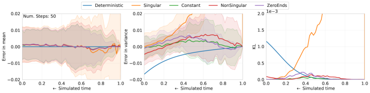
While infinitely many choices are available for , we consider a few interesting ones listed in the Table 1, constructed by choosing integer powers of and and introducing a scaling coefficient , for experimental evaluations. Note that the only degree of freedom in Table 1 is the choice of , which determines , given the flow field and the score . The is singular in Constant because the score , as computed in Equation 13, has in the denominator, making singular at . The choice in NonSingular precisely eliminates this singularity. Figure 2 compares these choices in a toy setup; Section 4 has comparisons on ImageNet.
3.3 Score function and classifier free guidance for a Gaussian flow model
Recall that Section 3.2 requires access to the score function. For Gaussian flows, the score function can be inferred from the velocity field itself, alleviating the need to learn it separately. This result is known (see e.g. Zheng et al. (2023) in the context of flow matching) and we present it here in our setting. For Gaussian flows, with and interpolation specified in Equation 1, the score can be computed as:
| (13) |
where is the estimated flow. Proof is provided in Appendix B. Note that the score function can also be estimated given or . In summary, the expression follows directly from using results from Denoising Score Matching (Vincent, 2011) and the Gaussianity of . Similar expressions can be derived for other interpolations that are linear in . With access to the score function and linearity of Equation 13 in we can define classifier free guided (Ho & Salimans, 2022) Gaussian flow as:
| (14) |
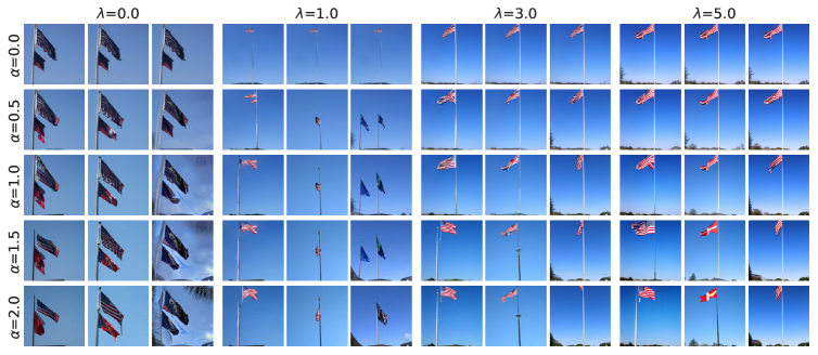
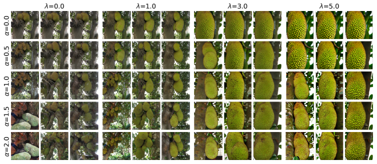
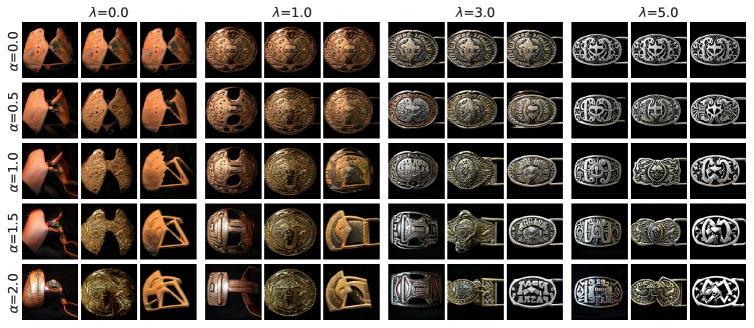
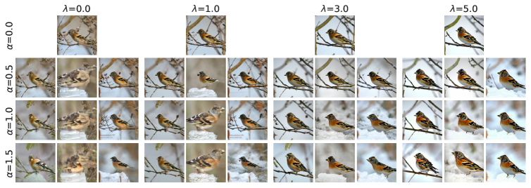
where indicates extra conditioning information as in classifier free guidance, indicates no conditioning and specifies the relative strength of the guidance. reduces to class conditional sampling, while puts a larger weight on the conditioning, biasing the sample towards the modes of the conditional distribution. Using classifier-free guidance with a stochastic sampler will, of course, give diversity that isn’t possible with a deterministic sampler, as can be seen in Figure 1. Note that Xie et al. (2024); Dao et al. (2023); Zheng et al. (2023) also consider related definitions in the context of flow matching.
4 Experiments
Our method allows us to identify a family of SDEs that correspond to a given deterministic Gaussian flow model, enabling construction of stochastic samplers with flexible diffusion coefficients. In our experiments we compare various samplers derived from the corresponding SDEs in Table 1, using Euler-Maruyama, for a given Gaussian flow model without any additional training.

4.1 Comparison on estimating marginal statistics for a two Gaussian toy problem
We start by considering a toy problem where both and are Gaussian. See Appendix G for details of the experimental setup and Appendix I for a JAX (Bradbury et al., 2018) implementation of NonSingular.
Discretization of deterministic flow leads to bias.
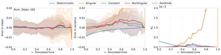
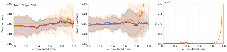
In Figure 2, with 50 sampling steps, we observe that the estimate for the mean is fairly accurate for all samplers for the entirety of the interval . However, the samplers differ in their behavior for variance. Deterministic exhibits a noticeable bias and underestimates the variance (with zero variance in its estimate), with the worst estimate at . Stochastic samplers provide noticeably better estimates at , but with increased variance.
Stochasticity is most helpful at coarser discretizations.
In Figure 3 we study the effect of the number of discretization steps on the different samplers (also see Figure 2 for 50 steps). While mean estimates are accurate for all methods, Deterministic gets increasingly biased for variance estimates as the number of sampling steps is decreased. Stochastic samplers perform consistently well at various discretization levels for , with significantly better estimates for fewer sampling steps. Note that Singular has very large bias as well as variance closer to ; those improve with finer discretization. Since Constant also has a singularity, but only in the drift term , we conclude that the instability is primarily due to the singularity in Singular’s diffusion term.
Stochasticity helps mitigate bias.
In Figure 4 we study the effect of diffusion coefficient scale on the NonSingular sampler at 100 sampling steps. Finite discretization introduces a bias in the deterministic sampler (when ), where the variance is consistently underestimated and is worst at . Increased stochasticity with increasing diffusion coefficient scale () helps mitigate this bias at the cost of increased variance. This can be seen in the figure with larger values yielding better estimate of the variance, although with larger variance in the estimate.
4.2 Comparison of SDEs for rectified flows on ImageNet generation
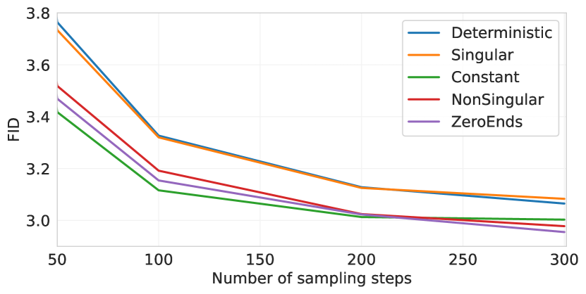
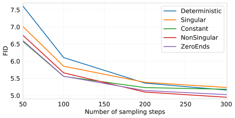
We compare the behavior of various SDEs on the sampling quality for large scale image generation using the ImageNet (2012) dataset (Deng et al., 2009; Russakovsky et al., 2015). We train rectified flow models at two different image resolutions ( and ) and compare their sample quality using the Frechet Inception Distance (FID) metric (Heusel et al., 2017) for class conditional samples. See Appendix H for setup details. The results show that small but statistically significant differences exist between samplers even for metrics like FID, but the optimal sampler is likely to be application and model specific.
Stochasticity can improve FID.
In Table 2 we report the best FID using each SDE in Table 1 for two image resolutions using 300 sampling steps, along with the corresponding diffusion term scale and one standard deviation confidence interval. Two key observations stand out: (1) stochastic samplers tend to produce better FIDs, and (2) the two non-singular samplers have much better FIDs than Deterministic or Singular. Note that observation (1) has also been made previously for probability flow ODEs (Song et al., 2020). The addition of a parameter to control the strength of the stochasticity while keeping the marginal distribution unchanged (Section 3.2), permits principled post-training optimization of the metrics like FID.
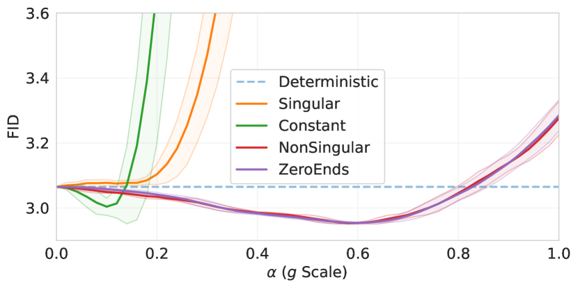
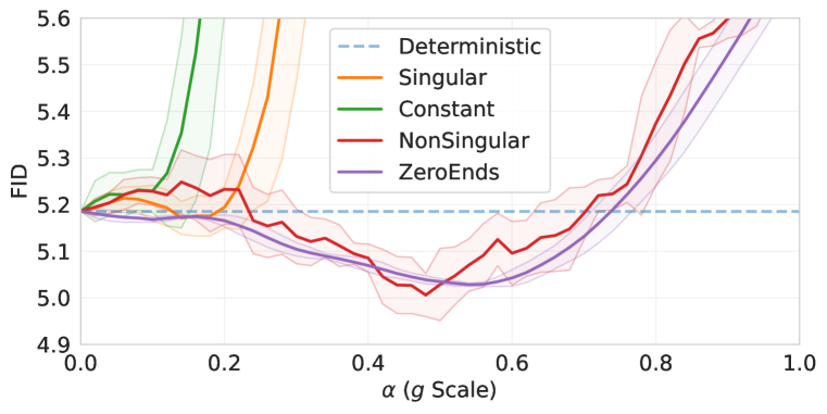
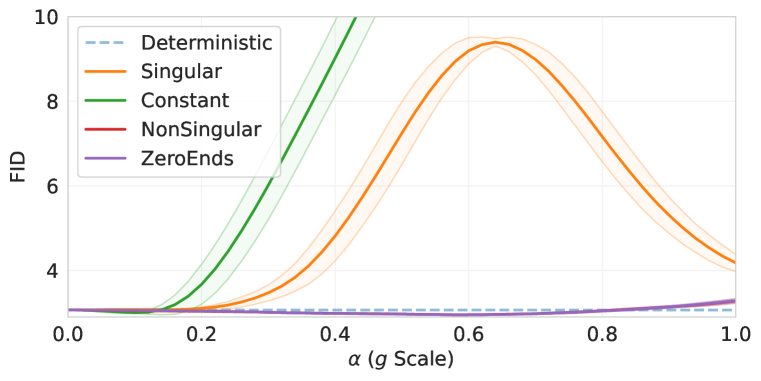
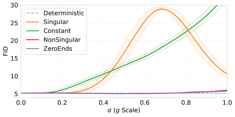
Non-singular samplers work well over a broad range of .
In Figures 5 and 7 we show how the FID varies with for each sampler for two different image resolution models. NonSingular and ZeroEnds attain better FID in general and are better behaved over a much larger range of the diffusion coefficient scale at both resolutions. These samplers both have small diffusion coefficients close to ; their performance indicates that noise near is particularly harmful. The low variance of ZeroEnds in comparison to NonSingular indicates that a large diffusion coefficient near tends to introduce variance in the final FID.
| Sampler | FID | FID | ||
|---|---|---|---|---|
| Deterministic | ||||
| Singular | ||||
| Constant | ||||
| NonSingular | ||||
| ZeroEnds | ||||
Stochasticity makes FID robust to discretization.
In Figure 6 we compare the effect of the number of sampling steps on FID for various samplers at two image resolutions. We set proportional to the number of sampling steps with the maximum value provided by Table 2. Again the non-singular samplers perform better than Deterministic at all discretization levels.
Stochastic sampling improves diversity at all classifier-free guidance levels.
In Figures 1 and 12 we show samples from NonSingular using classifier-free guidance (Section 3.3), varying both and , the guidance weight. In all cases, we can see that diversity increases with , and class typicality increases with .
Qualitative comparisons.
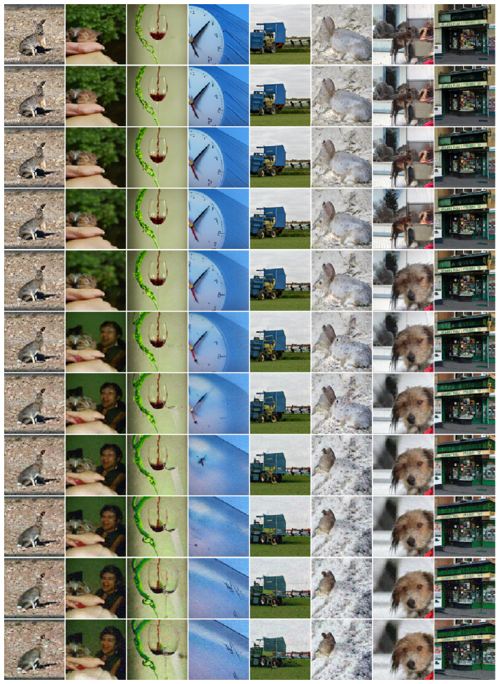
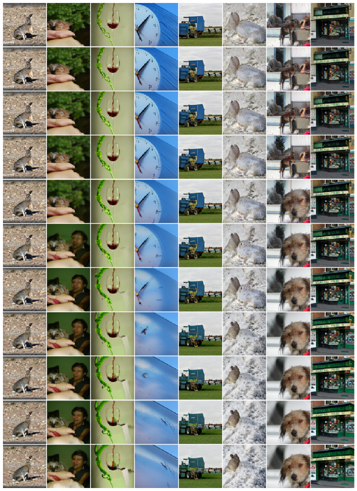
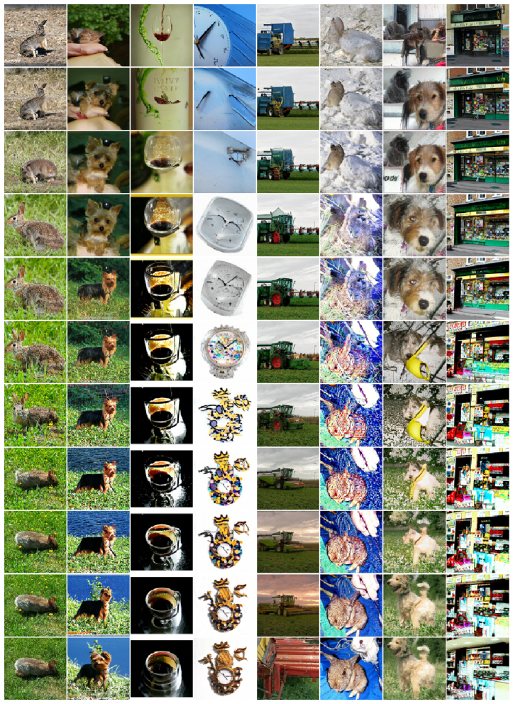
For qualitative comparisons, we visualize a few samples at various diffusion coefficient scales using different SDEs in Figures 9, 10 and 11. All samples in a column are generated by starting at the same draw ; different columns start from different draws. Noise scale gets progressively larger as we move down the rows. For Constant, we observe that samples get increasingly noisy with increasing indicating accumulating errors with increasing scale. The samples from NonSingular look better, as expected from Figure 5. Lastly, samples from Singular change much more rapidly in comparison to the other samplers, indicating that the singularities in the SDE coefficients increase the effect of noise.
5 Related work
Transport learning methods learn a mapping between two distributions, where the learned model can transform a sample from one distribution into a sample from the other one. Typically, one of the distributions is easy to sample (such as a Gaussian) and the other one is the data distribution that one is interested in modeling. The learned mapping can either be deterministic or stochastic. A thorough overview of related areas can be found in Yang et al. (2024).
Deterministic transport.
Deterministic transport methods implement a change of variable, either explicitly or approximately, that can be used to uniquely map a sample from one distribution to the other. The normalizing flow family (Rezende & Mohamed, 2015; Dinh et al., 2017; Kingma & Dhariwal, 2018) of methods construct an explicit invertible model that realizes this map either in one step or a finite number of discrete steps. Neural ODEs (Chen et al., 2018; Grathwohl et al., 2019) generalize from discrete steps to a continuous time mapping by inferring and learning the gradient field for all times. However, Neural ODEs are difficult to train due to the need for simulating the ODEs as part of the training. Rectified flows, flow matching, and iterative denoising methods (Liu et al., 2022; Lipman et al., 2022; Tong et al., 2023; Heitz et al., 2023; Delbracio & Milanfar, 2023) either implicitly or explicitly specify a continuous mapping and learn a model to approximate the continuous time mapping. Similarly, probability flow ODEs (Song et al., 2020) learned by diffusion models (Sohl-Dickstein et al., 2015) approximate an implicitly defined continuous mapping. Our work is useful for flexible sampling from such pre-trained continuous time deterministic Gaussian flows, or more generally where the score function for all the marginal distributions is either provided or can be deduced from the learned flow model.
Stochastic transport.
Stochastic transport methods learn a stochastic mapping, where a sample from one distribution gets stochastically mapped to a sample from the other. Gaussian diffusion models are a salient example of such discrete Sohl-Dickstein et al. (2015); Ho et al. (2020) or continuous time Song et al. (2020); Kingma et al. (2021) mappings where one of the distributions is constrained to be Gaussian. Several generalizations have been proposed that extend from Gaussian to more general families of distributions Yoon et al. (2024). The stochastic interpolants framework (Albergo & Vanden-Eijnden, 2022; Albergo et al., 2023; Ma et al., 2024) further generalizes to a larger family of distributions by introducing a random latent variable allowing efficient estimation of the score function at all times. Our work is directly applicable to models learned with such methods where the score function is accessible and can be used to construct and explore a large family of samplers. The convergence rates of diffusion models have been studied in Chen et al. (2023); Benton et al. (2023) with respect to the number of data samples and dimensionality. However, since our method does not require retraining, it does not affect these properties of the original training algorithms.
Schrödinger bridge and optimal transport.
These methods consider a more general problem of learning transport maps with additional constraints. k-Rectified flows Liu et al. (2022) provide an iterative procedure for tackling deterministic optimal transports for a family of costs, while the more general Schrödinger bridge problem, viewed as an entropy regularized optimal transport, is an active area of research Shi et al. (2024); Liu et al. (2023). Our work is complementary to these methods as we focus on flexible sampling, given the access to the score function for the marginal distributions.
6 Conclusion
We introduced a general method to identify a family of SDEs that have the same marginal distribution as a particular SDE, including the special case where the diffusion coefficient of the given SDE is zero. This special case corresponds to flow models which naively only support deterministic sampling. Our method enables flexible construction of stochastic samplers for such deterministic models where the diffusion coefficient can be chosen at sampling time from an infinitely large set of possibilities in an application and evaluation metric dependent way. Our method requires explicit access to the score function, in absence of which it is limited to a subset of flow models where the score function can be derived from the given flow model. However, this set includes currently popular rectified flow and diffusion models where one of the distributions is Gaussian.
References
- Albergo & Vanden-Eijnden (2022) Michael S Albergo and Eric Vanden-Eijnden. Building normalizing flows with stochastic interpolants. arXiv preprint arXiv:2209.15571, 2022.
- Albergo et al. (2023) Michael S Albergo, Nicholas M Boffi, and Eric Vanden-Eijnden. Stochastic interpolants: A unifying framework for flows and diffusions. arXiv preprint arXiv:2303.08797, 2023.
- Anderson (1982) Brian DO Anderson. Reverse-time diffusion equation models. Stochastic Processes and their Applications, 12(3):313–326, 1982.
- Benton et al. (2023) Joe Benton, Valentin De Bortoli, Arnaud Doucet, and George Deligiannidis. Linear convergence bounds for diffusion models via stochastic localization. arXiv preprint arXiv:2308.03686, 2023.
- Berner et al. (2022) Julius Berner, Lorenz Richter, and Karen Ullrich. An optimal control perspective on diffusion-based generative modeling. arXiv preprint arXiv:2211.01364, 2022.
- Bradbury et al. (2018) James Bradbury, Roy Frostig, Peter Hawkins, Matthew James Johnson, Chris Leary, Dougal Maclaurin, George Necula, Adam Paszke, Jake VanderPlas, Skye Wanderman-Milne, and Qiao Zhang. JAX: composable transformations of Python+NumPy programs, 2018. URL http://github.com/google/jax.
- Chen et al. (2023) Minshuo Chen, Kaixuan Huang, Tuo Zhao, and Mengdi Wang. Score approximation, estimation and distribution recovery of diffusion models on low-dimensional data. In International Conference on Machine Learning, pp. 4672–4712. PMLR, 2023.
- Chen et al. (2018) Ricky T. Q. Chen, Yulia Rubanova, Jesse Bettencourt, and David K Duvenaud. Neural ordinary differential equations. In S. Bengio, H. Wallach, H. Larochelle, K. Grauman, N. Cesa-Bianchi, and R. Garnett (eds.), Advances in Neural Information Processing Systems, volume 31. Curran Associates, Inc., 2018. URL https://proceedings.neurips.cc/paper_files/paper/2018/file/69386f6bb1dfed68692a24c8686939b9-Paper.pdf.
- Dao et al. (2023) Quan Dao, Hao Phung, Binh Nguyen, and Anh Tran. Flow matching in latent space. arXiv preprint arXiv:2307.08698, 2023.
- Delbracio & Milanfar (2023) Mauricio Delbracio and Peyman Milanfar. Inversion by direct iteration: An alternative to denoising diffusion for image restoration. arXiv preprint arXiv:2303.11435, 2023.
- Deng et al. (2009) Jia Deng, Wei Dong, Richard Socher, Li-Jia Li, Kai Li, and Li Fei-Fei. Imagenet: A large-scale hierarchical image database. In 2009 IEEE conference on computer vision and pattern recognition, pp. 248–255. Ieee, 2009.
- Dinh et al. (2017) Laurent Dinh, Jascha Sohl-Dickstein, and Samy Bengio. Density estimation using real NVP. In International Conference on Learning Representations, 2017. URL https://openreview.net/forum?id=HkpbnH9lx.
- Esser et al. (2024) Patrick Esser, Sumith Kulal, Andreas Blattmann, Rahim Entezari, Jonas Müller, Harry Saini, Yam Levi, Dominik Lorenz, Axel Sauer, Frederic Boesel, et al. Scaling rectified flow transformers for high-resolution image synthesis. arXiv preprint arXiv:2403.03206, 2024.
- Grathwohl et al. (2019) Will Grathwohl, Ricky T. Q. Chen, Jesse Bettencourt, and David Duvenaud. Scalable reversible generative models with free-form continuous dynamics. In International Conference on Learning Representations, 2019. URL https://openreview.net/forum?id=rJxgknCcK7.
- Heitz et al. (2023) Eric Heitz, Laurent Belcour, and Thomas Chambon. Iterative -(de) blending: A minimalist deterministic diffusion model. In ACM SIGGRAPH 2023 Conference Proceedings, pp. 1–8, 2023.
- Heusel et al. (2017) Martin Heusel, Hubert Ramsauer, Thomas Unterthiner, Bernhard Nessler, and Sepp Hochreiter. Gans trained by a two time-scale update rule converge to a local nash equilibrium. Advances in neural information processing systems, 30, 2017.
- Ho & Salimans (2022) Jonathan Ho and Tim Salimans. Classifier-free diffusion guidance. arXiv preprint arXiv:2207.12598, 2022.
- Ho et al. (2020) Jonathan Ho, Ajay Jain, and Pieter Abbeel. Denoising diffusion probabilistic models. Advances in neural information processing systems, 33:6840–6851, 2020.
- Hoogeboom et al. (2023) Emiel Hoogeboom, Jonathan Heek, and Tim Salimans. simple diffusion: End-to-end diffusion for high resolution images. In International Conference on Machine Learning, pp. 13213–13232. PMLR, 2023.
- Huang et al. (2021) Chin-Wei Huang, Jae Hyun Lim, and Aaron C Courville. A variational perspective on diffusion-based generative models and score matching. Advances in Neural Information Processing Systems, 34:22863–22876, 2021.
- Isola et al. (2017) Phillip Isola, Jun-Yan Zhu, Tinghui Zhou, and Alexei A. Efros. Image-to-image translation with conditional adversarial networks. In Proceedings of the IEEE Conference on Computer Vision and Pattern Recognition (CVPR), July 2017.
- Kawar et al. (2022) Bahjat Kawar, Michael Elad, Stefano Ermon, and Jiaming Song. Denoising diffusion restoration models, 2022.
- Kingma et al. (2021) Diederik Kingma, Tim Salimans, Ben Poole, and Jonathan Ho. Variational diffusion models. Advances in neural information processing systems, 34:21696–21707, 2021.
- Kingma & Ba (2014) Diederik P Kingma and Jimmy Ba. Adam: A method for stochastic optimization. arXiv preprint arXiv:1412.6980, 2014.
- Kingma & Dhariwal (2018) Durk P Kingma and Prafulla Dhariwal. Glow: Generative flow with invertible 1x1 convolutions. In Advances in Neural Information Processing Systems, volume 31. Curran Associates, Inc., 2018.
- Lipman et al. (2022) Yaron Lipman, Ricky TQ Chen, Heli Ben-Hamu, Maximilian Nickel, and Matt Le. Flow matching for generative modeling. arXiv preprint arXiv:2210.02747, 2022.
- Liu et al. (2023) Guan-Horng Liu, Arash Vahdat, De-An Huang, Evangelos A Theodorou, Weili Nie, and Anima Anandkumar. I2sb: Image-to-image schrödinger bridge. arXiv preprint arXiv:2302.05872, 2023.
- Liu et al. (2022) Xingchao Liu, Chengyue Gong, and Qiang Liu. Flow straight and fast: Learning to generate and transfer data with rectified flow. arXiv preprint arXiv:2209.03003, 2022.
- Loshchilov & Hutter (2017) Ilya Loshchilov and Frank Hutter. Decoupled weight decay regularization. arXiv preprint arXiv:1711.05101, 2017.
- Lu et al. (2022) Cheng Lu, Yuhao Zhou, Fan Bao, Jianfei Chen, Chongxuan Li, and Jun Zhu. Dpm-solver: A fast ode solver for diffusion probabilistic model sampling in around 10 steps, 2022.
- Lugmayr et al. (2022) Andreas Lugmayr, Martin Danelljan, Andres Romero, Fisher Yu, Radu Timofte, and Luc Van Gool. Repaint: Inpainting using denoising diffusion probabilistic models. In Proceedings of the IEEE/CVF Conference on Computer Vision and Pattern Recognition (CVPR), pp. 11461–11471, June 2022.
- Ma et al. (2024) Nanye Ma, Mark Goldstein, Michael S Albergo, Nicholas M Boffi, Eric Vanden-Eijnden, and Saining Xie. Sit: Exploring flow and diffusion-based generative models with scalable interpolant transformers. arXiv preprint arXiv:2401.08740, 2024.
- Meng et al. (2022) Chenlin Meng, Yutong He, Yang Song, Jiaming Song, Jiajun Wu, Jun-Yan Zhu, and Stefano Ermon. SDEdit: Guided image synthesis and editing with stochastic differential equations. In International Conference on Learning Representations, 2022. URL https://openreview.net/forum?id=aBsCjcPu_tE.
- Ramesh et al. (2022) Aditya Ramesh, Prafulla Dhariwal, Alex Nichol, Casey Chu, and Mark Chen. Hierarchical text-conditional image generation with clip latents, 2022.
- Rezende & Mohamed (2015) Danilo Rezende and Shakir Mohamed. Variational inference with normalizing flows. In Francis Bach and David Blei (eds.), Proceedings of the 32nd International Conference on Machine Learning, volume 37 of Proceedings of Machine Learning Research, pp. 1530–1538, Lille, France, 07–09 Jul 2015. PMLR.
- Rombach et al. (2022) Robin Rombach, Andreas Blattmann, Dominik Lorenz, Patrick Esser, and Björn Ommer. High-resolution image synthesis with latent diffusion models. In Proceedings of the IEEE/CVF Conference on Computer Vision and Pattern Recognition (CVPR), pp. 10684–10695, June 2022.
- Russakovsky et al. (2015) Olga Russakovsky, Jia Deng, Hao Su, Jonathan Krause, Sanjeev Satheesh, Sean Ma, Zhiheng Huang, Andrej Karpathy, Aditya Khosla, Michael Bernstein, Alexander C. Berg, and Li Fei-Fei. ImageNet Large Scale Visual Recognition Challenge. International Journal of Computer Vision (IJCV), 115(3):211–252, 2015. doi: 10.1007/s11263-015-0816-y.
- Saharia et al. (2022) Chitwan Saharia, William Chan, Saurabh Saxena, Lala Li, Jay Whang, Emily Denton, Seyed Kamyar Seyed Ghasemipour, Burcu Karagol Ayan, S. Sara Mahdavi, Rapha Gontijo Lopes, Tim Salimans, Jonathan Ho, David J Fleet, and Mohammad Norouzi. Photorealistic text-to-image diffusion models with deep language understanding, 2022.
- Särkkä & Solin (2019) Simo Särkkä and Arno Solin. Applied stochastic differential equations, volume 10. Cambridge University Press, 2019.
- Shi et al. (2024) Yuyang Shi, Valentin De Bortoli, Andrew Campbell, and Arnaud Doucet. Diffusion schrödinger bridge matching. Advances in Neural Information Processing Systems, 36, 2024.
- Sohl-Dickstein et al. (2015) Jascha Sohl-Dickstein, Eric Weiss, Niru Maheswaranathan, and Surya Ganguli. Deep unsupervised learning using nonequilibrium thermodynamics. In International conference on machine learning, pp. 2256–2265. PMLR, 2015.
- Song et al. (2020) Yang Song, Jascha Sohl-Dickstein, Diederik P Kingma, Abhishek Kumar, Stefano Ermon, and Ben Poole. Score-based generative modeling through stochastic differential equations. arXiv preprint arXiv:2011.13456, 2020.
- Tong et al. (2023) Alexander Tong, Nikolay Malkin, Guillaume Huguet, Yanlei Zhang, Jarrid Rector-Brooks, Kilian Fatras, Guy Wolf, and Yoshua Bengio. Improving and generalizing flow-based generative models with minibatch optimal transport. arXiv preprint arXiv:2302.00482, 2023.
- Vincent (2011) Pascal Vincent. A connection between score matching and denoising autoencoders. Neural computation, 23(7):1661–1674, 2011.
- Xie et al. (2024) Tianyu Xie, Yu Zhu, Longlin Yu, Tong Yang, Ziheng Cheng, Shiyue Zhang, Xiangyu Zhang, and Cheng Zhang. Reflected flow matching. arXiv preprint arXiv:2405.16577, 2024.
- Yang et al. (2024) Ling Yang, Zhilong Zhang, Yang Song, Shenda Hong, Runsheng Xu, Yue Zhao, Wentao Zhang, Bin Cui, and Ming-Hsuan Yang. Diffusion models: A comprehensive survey of methods and applications, 2024.
- Yoon et al. (2024) Eun Bi Yoon, Keehun Park, Sungwoong Kim, and Sungbin Lim. Score-based generative models with lévy processes. Advances in Neural Information Processing Systems, 36, 2024.
- Zheng et al. (2023) Qinqing Zheng, Matt Le, Neta Shaul, Yaron Lipman, Aditya Grover, and Ricky TQ Chen. Guided flows for generative modeling and decision making. arXiv preprint arXiv:2311.13443, 2023.
Appendix A Derivation of singular SDE
We consider the following SDE with additive noise; i.e., the diffusion coefficient is only a function of time.
| (15) |
The perturbation kernel corresponding to rectified flow is Gaussian, with . Since the perturbation kernel is Gaussian, following Song et al. (2020), we assume that the drift term is affine; i.e. . Further since are independent, we can directly infer the first and second moments for the marginals as and .
From Eq (5.50) of Särkkä & Solin (2019) we have
| (16) | ||||
| (17) |
where is the mean at time . Rearranging and integrating both sides:
| (18) | |||||
| (19) | |||||
| Differentiating both sides w.r.t. | (20) | ||||
Substituting , we get as in Equation 7:
| (22) |
Similarly, from Eq. (5.51) of Särkkä & Solin (2019):
| (23) |
Substituting (we are assuming isotropic dispersion), (symmetric, time-dependent diffusion coefficient), and from Equation 22:
| (24) | ||||
| (25) | ||||
| (26) | ||||
| (27) |
Above is an inhomogenous differential equation. The integrating factor can be calculated as:
| (28) |
Multiplying both sides of Equation 27, we can write:
| (29) |
Integrating both sides:
| (30) | ||||
| (31) |
Substituting :
| (32) |
Differentiating both sides w.r.t. and simplifying yields:
| (33) |
Substituting to the result in Equation 7:
| (34) |
Appendix B Score function from rectified flow
Given a base data distribution and a conditional noising distribution , Denoising score matching Vincent (2011) learns the score for the marginal by optimizing:
| (35) |
where . The solution to the above optimization problem can be written as:
| (36) |
Mapping the above to rectified flow with we get:
| (37) |
Next if:
| (38) | ||||
| (39) | ||||
| (40) |
Now:
| (41) |
Next, assume the covariance doesn’t depend on – i.e., – and the mean is linear in . Then:
| (42) | ||||
| (43) |
B.1 Gaussian Rectified Flow
Consider the special case where . We have . Using the result from Equation 43 we get:
| (44) |
From this, we can write:
| (45) | ||||
| (46) | ||||
| (47) | ||||
| (48) | ||||
| (49) | ||||
| (50) | ||||
| (51) | ||||
| (52) | ||||
| (53) | ||||
| (54) | ||||
| (55) |
B.2 General Rectified Flow
First recall the change of variables formula for a density with where is invertible and is differentiable:
| (56) |
Now, with and and , let be a function that is invertible in first argument and whose inverse is differentiable w.r.t. the first argument. Note that for simple rectified flows, satisfies these conditions.
We can now express the conditional density as:
| (57) |
The score for the conditional density can then be calculated as
| (58) |
and the score for the marginal density as:
| (59) | ||||
| (60) |
For the specific case of Rectified flows, define . Then:
| (61) | |||||
| Inverse is w.r.t. first argument | (62) | ||||
| (63) | |||||
| is | (64) | ||||
| (65) | |||||
Substituting into Equation 60:
| (66) |
It can be verified that with the choice of , we recover Equation 55.
Appendix C Proof of Section 3.2
*
Proof.
The evolution of the marginal probability density is then described by the Fokker-Planck-Kolmogorov (FPK) equation (Särkkä & Solin, 2019) as:
| (67) |
We write the above more succinctly as:
| (68) |
Where is the divergence operator. Next for an arbitrary consider the following identity:
| (69) | |||||
| (70) | |||||
| (71) | |||||
| (72) | |||||
Expanding out by substituting for :
| (73) | ||||
| (74) | ||||
Using Equation 72 and rewriting:
| (75) | ||||
Next we revisit Equation 68, and substitute for and with :
| (76) | ||||
| (77) | ||||
With cancellations, we arrive at:
| (78) |
which is the FPK equation describing the time evolution of the marginal probability density of the solutions of the SDE in Equation 4.
∎
Appendix D Proof of Section 3.2
*
Proof.
Starting with Theorem 1, let’s define and , where is a scalar valued function. These choices lead to following
| (79) | ||||
| (80) | ||||
| (81) | ||||
| (82) |
Note that Equation 81 follows from since neither nor are functions of . ∎
Appendix E Proof of Section 3.2
*
Proof.
First note that by definition from equation (3) in the paper. Now, again starting with Theorem 1, let’s define and , where is a scalar valued function. These choices lead to following
| (83) | ||||
| (84) | ||||
| (85) | ||||
| (86) |
Note that Equation 85 follows from since is not a function of . ∎
Appendix F Closed form rectified flow expression for the two Gaussian case
Our empirical studies use a two Gaussian toy problem setup. We state the closed form expression for the rectified flow for this case. Consider :
| (87) |
The marginal density is also Gaussian:
| (88) |
We have:
| (89) |
Using the following:
| (90) | ||||
| (91) |
and elementary properties of Gaussian and Dirac delta distributions, it can be verified that:
| (92) |
where .
Appendix G Toy Gaussian Experiment Details
In the experiments in Section 4.1 we study how various SDEs in Table 1 behave on a toy problem where both and are Gaussian. In this case the marginal distributions for Gaussian flow are Gaussian with and the true statistics can be easily computed. In addition, the rectified flow is available in closed form (see Appendix F). The SDEs are simulated backwards in time from with draws from using Equation 5. The drift and diffusion terms are calculated using Table 1 by setting and using the closed form from Equation 92. We simulate 10 trials of 10000 trajectories using Euler-Maruyama discretization with varying number of steps. Estimates for mean and variance at each timestep for various SDEs are calculated, along with their standard deviation across trials. Error, calculated as estimate - truth, is then plotted in Figures 2, 3 and 4 for both the mean and the variance estimates along with the KL-Divergence from the true marginal distribution.
Appendix H ImageNet experiment training/evaluation details
We train two base Rectified flow models to yield at two resolutions of 64 64 and 128 128, on the entire ImageNet training dataset containing roughly 1.2 million images. Our model is based on the architecture described in Hoogeboom et al. (2023). The model is structured such that the lower feature map resolution is 16 16. Therefore, for 64 64 resolution two downsamplings are performed, while for 128 128 three downsamplings are performed. The model is trained with SGD using adamw (Kingma & Ba, 2014; Loshchilov & Hutter, 2017) with for epochs. We use center crop and left-right flips as the only augmentations. An exponential moving average, with a decay of , of parameters is used for evaluation. FIDs are reported over the training dataset with reference statistics computed with center crop but without any augmentation, but with class conditioning. Samplers were evaluated for all .
The model trained for 500 epochs in 4 days, 8 hours on Google Cloud TPUs v3. The model trained for 500 epochs in 4 days, 20 hours on Google Cloud TPUs v3.
Appendix I Example Implementation
See Figure 8 for an example implementation of the NonSingular sampler.
Appendix J Additional Experimental Results
J.1 FID vs
J.2 Effect of diffusion coefficient magnitude on samples
We qualitatively visualize the effect of diffusion coefficient magnitude for the three SDEs discussed in the main paper. Figure 9 visualizes samples for the constant diffusion term SDE as a function increasing coefficient magnitude. Each column is a different sample starting with the same random draw from . Each row corresponds to a different magnitude for the diffusion coefficient . Figures 10 and 11 visualize samples with a similar scheme for the non-singular and singular SDE.
J.3 Classifier-free guidance samples
Figure 12 shows additional samples using classifier-free guidance with NonSingular at different values of and , as in Figure 1.