BackTime: Backdoor Attacks on
Multivariate Time Series Forecasting

Abstract

Multivariate Time Series (MTS) forecasting is a fundamental task with numerous real-world applications, such as transportation, climate, and epidemiology. While a myriad of powerful deep learning models have been developed for this task, few works have explored the robustness of MTS forecasting models to malicious attacks, which is crucial for their trustworthy employment in high-stake scenarios. To address this gap, we dive deep into the backdoor attacks on MTS forecasting models and propose an effective attack method named BackTime. By subtly injecting a few stealthy triggers into the MTS data, BackTime can alter the predictions of the forecasting model according to the attacker’s intent. Specifically, BackTime first identifies vulnerable timestamps in the data for poisoning, and then adaptively synthesizes stealthy and effective triggers by solving a bi-level optimization problem with a GNN-based trigger generator. Extensive experiments across multiple datasets and state-of-the-art MTS forecasting models demonstrate the effectiveness, versatility, and stealthiness of BackTime attacks. The code is available at https://github.com/xiaolin-cs/BackTime.

1 Introduction

Time series forecasting finds its applications across diverse domains such as climate [61, 34, 5, 25], epidemiology [13, 11, 56], transportation  [53, 63, 37, 29], and financial markets [51, 62, 42]. Multivariate time series (MTS) represent a collection of time series with multiple variables, and MTS forecasting aims to predict future data for each variable based on their historical data and the complex inter-variable relationship among them. Due to its wide applications and complexity, it has become an important research area. Many deep learning models have been developed to tackle this problem, including Transformer-based [67, 44, 58], GNN-based [24, 53, 22] and RNN-based [1, 26] models.

Despite the remarkable capacity of deep learning models, there is an alarming concern that they are susceptible to backdoor attacks [54, 21, 66, 41, 38]. The attack involves the surreptitious injection of triggers into datasets, causing poisoned models to provide wrong predictions when the inputs contain malicious triggers. Extensive works have shown that backdoor attack poses a serious risk across various classification tasks, including time series classification [30, 14]. However, the threat to time series forecasting remains unexplored and is of great importance to be investigated. For example, data-driven traffic forecasting systems are used in multiple countries to control traffic light timing, e.g., Google’s Project Green Light [20]. If the input signals to these forecasting systems are manipulated by hackers to provide malicious predictions, it could lead to widespread traffic congestion and thus brings negative economic and societal impacts. Similar situations, such as attacks to stock prediction [6, 51, 64] and climate forecasting [49, 50, 52, 23], would significantly weaken the reliability of forecasting models and do great harm.

To address this critical and imminent issue, we extend the application landscape of backdoor attack from MTS classification to forecasting. Unlike traditional backdoor attacks that focus on specific class labels, our approach aims to induce poisoned models to predict future data as a predefined target pattern. This new problem prompts several questions that deserve exploration in this paper: First, stealthy attack, i.e., to what extent can such a manipulation on datasets be imperceptible by minimizing the amplitude of triggers and maintaining a low injection rate [38, 18]? Second, sparse attack, i.e., how can data manipulation be confined to a small subset of variables within MTS [39]?

In this paper, we present a novel generative framework for generating stealthy and sparse attacks on MTS forecasting. To begin with, we first describe a threat model that introduces attackers’ abilities and goals, paving the way for formally defining the problem of MTS forecasting attacks. Then, to realize the conceptual attackers, we formalize the trigger generation within a bi-level optimization process and design an end-to-end generative framework called BackTime, which adaptively constructs a graph that measures inter-variable correlations and iteratively solves the bi-level optimization by employing a GNN-based trigger generator. The intuition behind this is that triggers effective for one variable are likely to be successful in attacking similar variables. During the optimization, generated triggers can be sparsely added to only a subset of variables, thereby only altering the model’s prediction behavior for these target variables. Moreover, to ensure the stealthiness of the attack, we introduce a non-linear scaling function into the trigger generator to limit the amplitude of triggers and also leverage a shape-aware normalization loss to ensure that the frequency of the generated triggers closely match those of the normal time series data.

In summary, our main contributions are as follows:

• Problem. To the best of our knowledge, we are the first to extend the concept of backdoor attacks to MTS forecasting. We identify two crucial properties of backdor attacks on MTS forecasting: stealthiness and sparsity; and further devise a novel threat model on this basis.

• Methodology. We propose a bi-level optimization framework for backdoor attacks on MTS forecasting, aiming to generate effective triggers under stealthy constraints. Based on this framework, we leverage a GNN-based trigger generator to design triggers based on the inter-variable correlations.

• Evaluation. We conduct extensive experiments on five widely used MTS datasets, demonstrating that BackTime achieves state-of-the-art (SOTA) backdoor attack performance. Our results show that BackTime can effectively control the attacked model to give predictions according to the attacker’s intent when faced with poisoned inputs, while maintaining its high forecasting ability for clean inputs.

2 New Backdoor Attack Setting for MTS Forecasting

2.1 Preliminary

Multivariate time series forecasting. In multivariate time series, the dataset encompasses time series with multiple variables, denoted as $\mathbf{X}=\{\mathbf{x}_{1},\mathbf{x}_{2},\dots,\mathbf{x}_{N}\}\in\mathbb{R}^{T\times N}$ where $T$ represents the time spans, $N$ represents the number of variables, and $\mathbf{x}_{i}$ is the time series sequence of the $i$-th variable. For forecasting tasks, a widely used method for training is to slice time windows from the dataset as the training inputs. Let $t^{\texttt{IN}}$ denote the length of time windows. Then for any timestamp $t_{i}$ , the input will consist of historical sequences spanning from timestamps $t_{i}-t^{\texttt{IN}}$ to $t_{i}$, expressed as $\mathbf{X}[t_{i}-t^{\texttt{IN}}:t_{i}]$ . The objective of MTS forecasting is to predict future time series denoted $\mathbf{X}[t_{i}:t_{i}+t^{\texttt{OUT}}]$ where $t^{\texttt{OUT}}$ represents the prediction timestamp. In the following paper, we use $\mathbf{X}_{t_{i},h}$ to represent historical data $\mathbf{X}[t_{i}-t^{\texttt{IN}}:t_{i}]$ and $\mathbf{X}_{t_{i},f}$ to represent future data $\mathbf{X}[t_{i}:t_{i}+t^{\texttt{OUT}}]$ for notation convenience. The main notations in this paper are listed in Table 5.

Backdoor Attacks on Classifications Traditional backdoor attacks have proven highly effective in classification tasks across diverse data formats. Given a dataset $\mathcal{D}=\{\mathcal{X},\mathcal{Y}\}$ with $\mathcal{X}$ and $\mathcal{Y}$ representing the set of samples (e.g., images, text, time series) and corresponding labels, respectively, attackers generate some special and commonly invisible patterns, which are called triggers. For example, triggers could be specific pixels in images, [21, 54, 8], particular sentences in text [35, 48, 9], and designed perturbations on time series [30, 14]. These triggers are then inserted into a small subset of samples in $\mathcal{D}$, with their labels flipped to a predefined target label. After training on the poisoned dataset, models will predict the class as the target label if the inputs contain triggers while still performing normally when facing clean inputs, i.e., the inputs without triggers.

2.2 Differences from Attacks on Forecasting w.r.t Tasks and Data Formats

Compared with the traditional backdoor attack [8, 54, 21, 30, 14, 35, 48], the backdoor attack on MTS forecasting bears several important and unique challenges, as shown in Table 1.

Table 1: Comparisons of the backdoor attack on MTS forecasting and other backdoor attack tasks.

Backdoor Attack Paradigm	Task-wise Challenges				Data-wise Challenges
	Target	Real-time	Constraint on	Soft	Human	Inter-variable
	Object	Attack	Target Object	Indentification	Unreadability	Dependence
Image/Text Classification [21, 54, 35, 48]	Discrete scalar (label)	$\times$	$\times$	$\times$	$\times$	$\times$
Univariate Time Series Classification [14, 30]	Discrete scalar (label)	$\times$	$\times$	$\times$	$\checkmark$	$\times$
Multivariate Time Series Classification [14, 30]	Discrete scalar (label)	$\times$	$\times$	$\times$	$\checkmark$	$\checkmark$
Multivariate Time Series Forecasting (Ours)	Sequence (pattern)	$\checkmark$	$\checkmark$	$\checkmark$	$\checkmark$	$\checkmark$

Considering tasks, traditional backdoor attack is applied for classification while this paper focuses on forecasting, which in turn brings the following four crucial differences. (1) Target object. Instead of flipping labels on classification, we concatenate triggers and target patterns into successive sequences and inject them together into the training set, thus building strong temporal correlations between triggers and target patterns. (2) Real-time attack. Unlike traditional backdoor attacks which may leverage ground truth data for trigger generation, the attack on forecasting is only allowed to use the historical data due to the timeliness. For example, if a hacker aims to alter the traffic flow data to reach a specific value at time $t_{i}$, then this specific value should be determined before $t_{i}$. Otherwise, the data manipulation will be too late and thus useless, since the traffic flow data would have already been sent to the forecasting system in real-time. It indicates that the shape of triggers at the timestamp of $t_{i}$ should be known ahead of $t_{i}$. Therefore, the generation of triggers can only utilize data of $t_{i}-1$ at most. (3) Constraint on target object. On MTS forecasting, since both the triggers and the target pattern are injected into the dataset, we need to impose constraints on triggers as well as the target pattern. (4) Soft identification. Since perhaps only a part of triggers and target patterns are retained in sliced time windows, a novel soft identification mechanism is needed to determine if a window has been attacked. Detailed explanations of (3) and (4) are provided in Section 3.1.

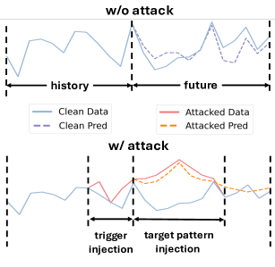
Figure 1: An illustrative example of data poisoning on the PEMS03 dataset. After triggers and target patterns (red lines) are injected, predictions of the attack model (orange dash line) will resemble the target pattern.

Considering data, MTS data bears the following uniqueness. (1) Human unreadability. Analyzing time series data often requires specialized knowledge, like financial expertise for stock prices. This makes it harder for humans to detect modifications in time series data compared to images or texts. Hence, human judgments is not reliable for assessing the stealthiness of backdoor attack on forecasting. As a result, we leverage anomaly detection methods as the stealthiness indicator, since if a trigger is not stealthy, it will differ significantly from the original data, making it detectable as an anomaly. (2) Inter-variable dependence. Compared with univariate time series, the attack on MTS data are much more complicated due to the inter-variable correlations. Since advanced forecasting models [58, 68, 7, 24, 67] tend to leverage correlations between variables to enhance their forecasting performances, if a trigger can successfully attack the prediction of one variable, similar triggers might also work for closely correlated variables. Thus, trigger generation must consider both temporal dependencies and inter-variable correlations.

Based on all these differences, we present the detailed treat model of backdoor attack on MTS forecasting as follows.

2.3 Threat Model of Attacks on MTS Forecasting

Capability of attackers: Given a training dataset, the attacker can select $\alpha_{\texttt{T}}$ timestamps to poison, denoted as $\mathcal{T}^{\texttt{ATK}}$. Then, for each timestamp $t_{i}\in\mathcal{T}^{\texttt{ATK}}$, the attacker generates an invisible trigger $g\in\mathbb{R}^{t^{\texttt{TGR}}\times|\mathcal{S}|}$, where $t^{\texttt{TGR}}$ denotes the length of the trigger, and $\mathcal{S}\subseteq\{1,\ldots,N\}$ denotes the selected variables to poison. After that, the attacker starts to poison the corresponding time series by injecting the trigger, i.e., $\textbf{X}\left[t_{i}-t^{\texttt{TGR}}:t_{i},\mathcal{S}\right]\leftarrow\textbf{X}\left[t_{i}-t^{\texttt{TGR}}-1,\mathcal{S}\right]\oplus g$, and also replacing the future data with the target pattern, i.e., $\textbf{X}\left[t_{i}:t_{i}+t^{\texttt{PTN}},\mathcal{S}\right]=\textbf{X}\left[t_{i}-t^{\texttt{TGR}}-1,\mathcal{S}\right]\oplus p$, where $\oplus$ represents the addition with Python broadcasting mechanism, and $t^{\texttt{PTN}}$ is the length of a predefined target pattern. The data poisoning example is illustrated in Figure 1.

Goals of attackers: (1) Attacked forecasting models predict the future as the ground truth when facing clean inputs. (2) Attacked forecasting models predicts the future of the target variables as the given target pattern when the poisoned historical data contains triggers.

2.4 Formal Problem Definition

Problem 1

Backdoor attacks on multivariate time series forecasting.

Input: (1) a clean dataset $\textbf{X}\in\mathbb{R}^{T\times N}$ where $T$ represents the time span and $N$ represents the number of variables; (2) a predefined target pattern $p$ with a length of $t^{\texttt{PTN}}$; (3) the length $t^{\texttt{TGR}}$ of triggers to be added, (4) a temporal injection rate $\alpha_{\texttt{T}}$, and (5) a set of target variables $\mathcal{S}$ satisfying $\frac{|\mathcal{S}|}{N}\geq\alpha_{\texttt{S}}$ with $\alpha_{\texttt{S}}$ being the spatial injection rate.

Output: a poisoned dataset $\mathbf{X}^{\texttt{ATK}}$ by poisoning $\alpha_{\texttt{T}}$ timestamps such that the performances of attacked models will align with goals of attackers if models are trained on a poisoned dataset.

3 Backdoor Attacks on MTS Forecasting

In this section, we introduce our comprehensive threat model proposed for backdoor attacks on MTS forecasting. First, we formalize the general objective of our threat model in Section 3.1. Then, we introduce how to instance this objective with our BackTime in Section 3.2.

3.1 General Goal and Formulation

In this section, we propose two unique designs for backdoor attacks on MTS forecasting based on the key differences discussed in Section 2.2.

Stealthiness constraints on triggers and target patterns. To uphold stealthiness in backdoor attacks, it is imperative to ensure that the poisoned data closely resembles the ground truth data [30, 38, 57]. However, as Section 2 shows, the insertion of triggers is intended to be applied on the unknown future. This design limitation makes it almost impossible to ensure the similarity between the poisoned data and the unknown future. To alleviate this issue, we consider the similarity between the poisoned data and the recent historical data as a pragmatic alternative, indicating that the amplitude of generated triggers should be controlled under a small budget. In addition, the same constraint is supposed to be utilized on target patterns since target patterns are also integrated into the training data. Mathematically, we use $L_{\infty}$ norm for stealthiness constraints like [16, 15]. Therefore, the stealthiness constraints could be formally written as:

$$\|g\|_{\infty}\leq\varDelta^{\texttt{TGR}},\quad\|p\|_{\infty}\leq\varDelta^{\texttt{PTN}}$$ (1)

where $\varDelta^{\texttt{TGR}}$ and $\varDelta^{\texttt{PTN}}$ are the budgets for triggers and target patterns, respectively.

Soft identification on poisoned samples. In Multivariate Time Series (MTS) forecasting, a common practice [58, 27, 68, 7] involves slicing datasets into time windows to serve as inputs for forecasting models. However, in a poisoned dataset $\mathbf{X}^{\texttt{ATK}}$, identifying whether these sliced time windows are poisoned poses significant challenges for two primary reasons. First, the length of these time windows may not align with the length of triggers or target patterns. Second, when slicing datasets into time windows, these windows may encompass only a fraction of the triggers or target patterns. To solve these problems, we propose a soft identification mechanism. Specifically, we assume that the injected backdoor is activated only when inputs encompass all components of the triggers. Furthermore, we define the degree of poisoning in inputs based on the proportion of target patterns within the future to be forecasted. The rationale behind is that when the backdoor begins to be activated, its influence should be most pronounced, resulting in a significant impact on the forecasting process. As time goes, the strength of this effect gradually diminishes since the proportion of target patterns within the future decreases. Mathematically, for any timestamp $t_{i}$, the soft identification mechanism is formalized as follows:

$$\beta(t_{i})=\eta\left(\frac{c^{\texttt{PTN}}_{t_{i}}}{t^{\texttt{PTN}}}\right)\mathds{1}\left(c^{\texttt{TGR}}_{t_{i}}=t^{\texttt{TGR}}\right)$$ (2)

where $\beta(t_{i})$ represents the soft identification mechanism at the timestamp $t_{i}$, $c^{\texttt{TGR}}_{t_{i}}$ and $c^{\texttt{PTN}}_{t_{i}}$ are the length of triggers within $\mathbf{X}^{\texttt{ATK}}_{t_{i},h}$ and target patterns within $\mathbf{X}^{\texttt{ATK}}_{t_{i},f}$ , respectively. $\eta$ is a monotonically decreasing function satisfying $\eta(1)=1$ and $\eta(0)=0$, which measures the significance attributed to the degree of poisoning. For example, if $\eta$ rapidly decreases within the range of $(0,1)$, it implies that once the triggers are activated, the expected effects of triggers will diminish rapidly over time.

To sum up, we refine the basic optimization problem [15, 16] of typical backdoor attack by integrating the above adjustments, hence providing a general mathematical framework for backdoor attack on MTS forecasting:

$$\min_{g} \mathbb{E}_{t_{i}\sim\mathcal{T}}\left[\mathcal{L}_{\texttt{ATK}}\left(f\left(\mathbf{X}^{\texttt{ATK}}_{t_{i},h};\theta^{*}\right),\mathbf{X}^{\texttt{ATK}}_{t_{i},f}\right)\cdot\beta(t_{i})\right]$$ (3)

$$\mathrm{s.t.\;\,} \,\theta^{*}=\operatorname{argmin}\mathbb{E}_{t_{i}\sim\mathcal{T}}\left[\mathcal{L}_{\texttt{CLN}}\left(f\left(\mathbf{X}^{\texttt{ATK}}_{t_{i},h};\theta\right),\mathbf{X}^{\texttt{ATK}}_{t_{i},f}\right)\right],$$

$$\|g\|_{\infty}\leq\varDelta^{\texttt{TGR}},\quad\|p\|_{\infty}\leq\varDelta^{\texttt{PTN}}.$$

where $\mathbf{X}^{\texttt{ATK}}$ represents the poisoned dataset, $\mathcal{T}$ represents the set of timestamps in $\mathbf{X}^{\texttt{ATK}}$, $f(\cdot)$ denotes the forecasting model with its parameters of $\theta$, $\mathcal{L}_{\texttt{CLN}}$ is the clean loss for forecasting tasks, and $\mathcal{L}_{\texttt{ATK}}$ is the attack loss designed to make the model’s output resemble the target pattern. The key idea here is that, after a model is trained on the poisoned dataset $\mathbf{X}^{\texttt{ATK}}$ through the lower-level optimization, we aim to minimize the expectation of difference between the output of this model and the target pattern, as shown in the upper-level optimization. This is based on the fact that in the upper optimization, $\mathbf{X}^{\texttt{ATK}}_{t_{i},f}$ contains at least a part of the target pattern $g$ when $\beta(t_{i})\neq 0$. Additionally, although constraints are imposed on both the triggers and the target pattern, the constraint on the target pattern does not actively participate in the optimization process. Instead, it serves as a constraint that the attacker is expected to adhere to when determining the shape of the target pattern.

3.2 BackTime Algorithm

To successfully achieve backdoor attack on MTS forecasting, we need to determine three key elements: (RQ1) where to attack, i.e., identifying which variable to target; (RQ2) when to attack, i.e., selecting which timestamps to attack; and (RQ3) how to attack, i.e., specifying the trigger to inject. Regarding (RQ1) where to attack, as outlined in Problem 1, the target variables are determined by the attacker and can be any variable desired. Subsequently, we will discuss (RQ2) when to attack in Section 3.2.1, and provide the details of (RQ3) how to attack in Sections 3.2.2 and 3.2.3.

3.2.1 Selecting Timestamps for Poisoning

In this section, we design an illustrative experiment to investigate the properties of the timestamps that are more susceptible to attack. The main idea of the experiment is, given a simple and weak backdoor attack, to observe the change of attack effect when choosing timestamps with different properties for attack. Based on the experiment results, we find that timestamps w.r.t. high prediction errors for a clean model are more susceptible to attacks.

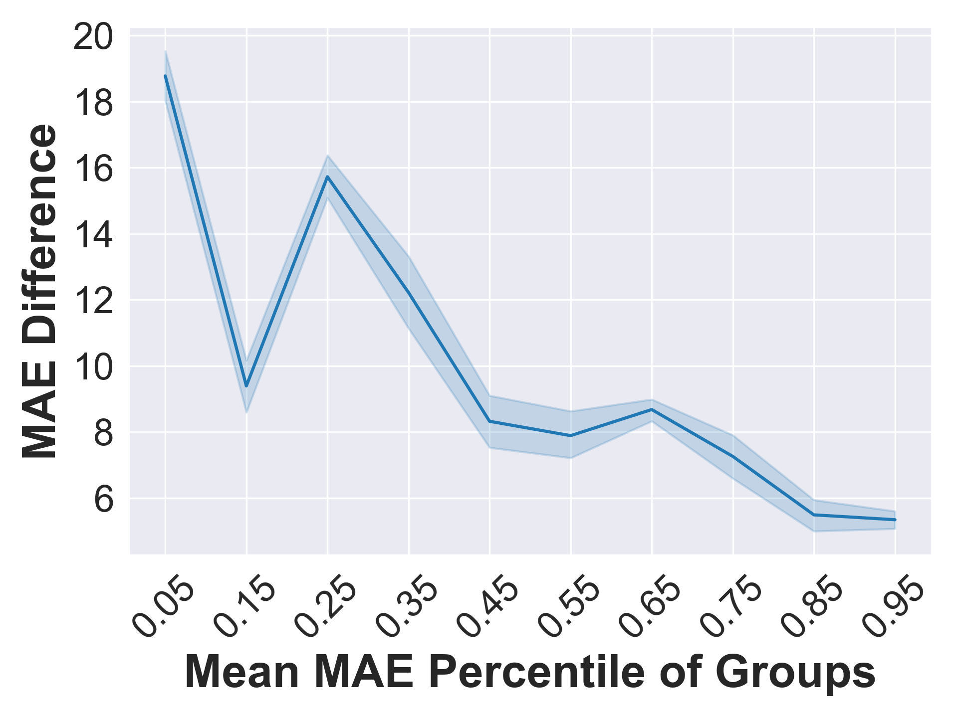
Figure 2: The difference of MAE between a clean model and an attacked model when using different timestamps for attack. A lower MAE difference (y-axis) indicates more susceptible timestamps to attack.

We investigate the properties of timestamps on the PEMS03 dataset. Specifically, we first train a forecasting model (i.e., clean model $f^{\texttt{CLN}}$) on the original dataset $\mathbf{X}$ and record the Mean Absolute Error (MAE) of the predictions for each timestamp. A higher MAE indicates poorer prediction performance for that timestamp. We then sort the timestamps in ascending order based on their MAE and divide them into ten groups, with average MAE percentiles of $0.05,0.15,\cdots,0.95$, as shown on the x-axis of Figure 2. Then, for each group, we implement a simple backdoor attack, where a shape-fixed trigger and target pattern are injected to all the timestamps and variables within the timestamp group, and train a new model (i.e., attacked model $f^{\texttt{ATK}}$) on the poisoned data $\mathbf{X}^{\texttt{ATK}}$. The shapes of the trigger and the target pattern are shown in Appendix D. Intuitively, a timestamp $t_{i}$ that is susceptible to backdoor attack will have a low poisoned MAE, i.e., $\texttt{MAE}(f^{\texttt{ATK}},\mathbf{X}^{\texttt{ATK}}_{t_{i},h},\mathbf{X}^{\texttt{ATK}}_{t_{i},f})$. It means that at timestamp $t_{i}$, the predictions of the attacked model can be greatly altered by the attack to fit the target pattern. However, relying solely on poisoned MAE is insufficient because if the target pattern closely resembles the ground truth, the poisoned MAE will still be low even if the attack fails. To address this problem, we test a clean model on the poisoned dataset and further record its clean MAE for each poisoned timestamp $t_{i}$, i.e., $\texttt{MAE}(f^{\texttt{CLN}},\mathbf{X}^{\texttt{ATK}}_{t_{i},h},\mathbf{X}^{\texttt{ATK}}_{t_{i},f})$. Then, a lower MAE difference between poisoned MAE and clean MAE can reliably indicate more vulnerable timestamps, since the clean MAE will be quite low, leading to a high MAE difference, when the target pattern is similar to the ground truth. The experiment results, as shown in Figure 2, demonstrate that the group with higher MAE percentile can continuously lead to a lower MAE difference. These findings imply that timestamps where a clean model performs poorly are more susceptible to backdoor attacks. Therefore, to ensure the strength of backdoor attack, for each timestamp $t_{i}$, we leverage a pretrained clean model to calculate MAE between predictions and the ground truth $\mathbf{X}_{t_{i},f}$, and further select the top $\alpha_{\texttt{T}}$ timestamps with the highest MAE, denoted as $\mathcal{T}^{\texttt{ATK}}$.

3.2.2 Trigger Generation

Once the poisoned timestamps are determined, the next step is to generate adaptive triggers to poison the dataset. First, we generate a weighted graph by leveraging an MLP to capture the inter-variable correlation within the target variables $\mathcal{S}$. Then, we further utilize a Graph Convolutional Network (GCN) [32] for trigger generation based on the learned weighted graph.

Graph structure generation. Since we aim to activate backdoor in any timestamps, we do not expect that the generated graph is closely related to specific local temporal properties in the training set. Thus, we focus on building a static graph by learning the global temporal features within the target variables $\mathcal{S}$. Motivated by this goal, we take as the entire input time series data $\mathbf{x}_{i},i\in\mathcal{S}$ instead of using sliced time windows. However, the time span $T$ of time series data is often very large, and hence it is inefficient to directly use total data without preprocessing. Therefore, we apply the discrete Fourier transform (DFT) [45] to effectively reduce the dimension while maintaining useful information. Intuitively, long-time-scale features, such as trends and periodicity, play a pivotal role in the global temporal correlation among variables, compared with the local noise or high-frequency fluctuations. Consequently, after DFT, we retain only the low-frequency features of the time series data. Mathematically, for any target variable $i\in\mathcal{S}$, this transform could be expressed as $\mathbf{z}_{i}=\operatorname{Filter}(\operatorname{DFT}(\mathbf{x}_{i}),k)$ where $\operatorname{DFT(\cdot)}$ represents the DFT transformation, and $\operatorname{Filter}(\cdot,k)$ represents preserving the top $k$ low-frequency features. Furthermore, we employ Multilayer Perceptron (MLP) to adaptively learn features of different frequencies. Subsequently, we utilize the output of the MLP to construct a graph that measures the correlation between target variables. The aforementioned process can be expressed as:

$$\mathbf{A}_{i,j}=cos(\operatorname{MLP}(\mathbf{z}_{i}),\operatorname{MLP}(\mathbf{z}_{j})),\;i,j\in\mathcal{S}$$ (4)

where $\mathbf{A}_{i,j}$ represents the element of learned graph $\mathbf{A}$ at the $i$-th row and the $j$-th column, and $cos(\cdot,\cdot)$ represents the cosine similarity.

Adaptive trigger generation. Once a correlation graph has been obtained, our objective shifts to the generation of learnable triggers that can be seamlessly integrated into various models with efficacy and imperceptibility. To ensure semantic consistency between triggers and historical data, we employ a time window with a length of $t^{\texttt{BEF}}$ to slice the historical data preceding the trigger. Then, we utilize a GCN for trigger generation based on the sliced historical data:

$$\hat{g}_{t_{i}}=\operatorname{GCN}(\mathbf{X}^{\texttt{ATK}}[t_{i}-t^{\texttt{BEF}}-t^{\texttt{TGR}}:t_{i}-t^{\texttt{TGR}},\mathcal{S}],\mathbf{A}),\;\forall\,t_{i}\in\mathcal{T}^{\texttt{ATK}}$$ (5)

In experiments, we find the following phenomenon: the GCN intends to aggressively increase the amplitude of output $\hat{g}_{t_{i}}$. Even if an extra penalty on the amplitude is introduced, it still requires much effort to adjust the hyperparameters to control the trigger amplitude. One potential explanation for this behavior is that a large trigger amplitude leads to substantial deviation, and data points characterized by such deviations are more readily learned by forecasting models although they violate the requirements of stealthiness. To address this issue, we propose to introduce a non-linear scaling function, $tanh(\cdot)$, to generate stealthy triggers by imposing mandatory limitations on the amplitude of outputs $\hat{g}_{t_{i}}$. Mathematically, the generated triggers can be formalized as follows:

$$g_{t_{i}}=\varDelta^{\texttt{TGR}}\cdot tanh(\hat{g}_{t_{i}}),\;\forall t_{i}\in\mathcal{T}^{\texttt{ATK}}$$ (6)

3.2.3 Bi-level Optimization

After introducing the model architecture of the adaptive trigger generator $f_{g}$ in Eqs. (5) and (6), we aim to optimize the trigger generator through a bi-level optimization problem in Eq. (3) to ensure the effectiveness of the generated triggers. Recognizing the inherent complexity of bi-level optimization, we introduce a surrogate forecasting model $f_{s}$ to provide a practical approximation of the precise solution. This allows us to solve Eq. (3) by iteratively updating the surrogate model and the trigger generator. However, we further find that if we randomly initialize the surrogate model $f_{s}$, then the performance of the trigger generator tends to fluctuates in the initial stage, posing a significant difficulty in convergence. Therefore, we introduce an additional warm-up phase. During the warm-up phase, we only train the surrogate model to make it have a reasonable forecasting ability. Once the warm-up phase is over, we will update both the surrogate model and trigger generator. Specifically, in this phase, we will divide the training process for each epoch into two stages: (1) the surrogate model update, and (2) the trigger generator update.

Input : A MTS dataset $\mathbf{X}$, a surrogate forecasting model $f_{s}$, a trigger generator $f_{g}$, a temporal injection rate $\alpha_{\texttt{T}}$, and a set of target variables $\mathcal{S}$

Output : A poisoned dataset $\mathbf{X}^{\texttt{ATK}}$

1 Initialize $\mathcal{T}$ as the set of timestamps in $\mathbf{X}$

// Warm-up phase

2 Train $f_{s}$ on $\mathbf{X}$ for $epoch_{warm}$ epochs

// Selecting poisoned timestamps

3 $s_{t_{i}}\leftarrow\operatorname{MAE}(f_{s}(\mathbf{X}_{t_{i},h}),\mathbf{X}_{t_{i},f}),\;\forall t_{i}\in\mathcal{T}$;

4 $\mathcal{T}^{\texttt{ATK}}\leftarrow$ top $\alpha_{\texttt{T}}$ timestamps with highest $s_{t_{i}}$;

// Bi-level training phase

5 for $epoch=1\rightarrow epoch_{train}$ do

6       Update $g_{t_{i}}$ w.r.t. Eq. (6) and get $\mathbf{X}^{\texttt{ATK}}$;

7       Update $f_{s}$ w.r.t. Eq. (7);

8       Update $f_{g}$ w.r.t. Eqs. (8), (9) and (10);

9      

10Update $g_{t_{i}}$ w.r.t. Eq. (6) and get $\mathbf{X}^{\texttt{ATK}}$;

return $\mathbf{X}^{\texttt{ATK}}$;

Algorithm 1 BackTime

At the first stage, we poison the clean dataset, as mentioned in Section 2.3. Then we aim to improve the forecasting ability of the surrogate model $f_{s}$ on the poisoned dataset $\mathbf{X}^{\texttt{ATK}}$. Specifically, we employ a natural forecasting loss function, denoted as $\mathcal{L}_{\texttt{CLN}}$, to update the surrogate model $f_{s}$ while fixing the parameters of the trigger generator $f_{g}$:

$$l_{cln}=\mathcal{L}_{\texttt{CLN}}\left(f_{s}\left(\mathbf{X}^{\texttt{ATK}}_{t_{i},h}\right),\mathbf{X}^{\texttt{ATK}}_{t_{i},f}\right),\;\forall t_{i}\in\mathcal{T}$$ (7)

In this paper, we use smooth $L_{1}$ loss [28] as the forecasting loss $\mathcal{L}_{\texttt{CLN}}$.

As for the second stage, we aim to update the trigger generator $f_{g}$ for effective and unnoticeable triggers. Following Section 2.3, for each poisoned timestamp $t_{i}\in\mathcal{T}^{\texttt{ATK}}$, we will utilize the trigger generator $f_{g}$ to obtain the trigger $g_{t_{i}}$ based on Eqs (5) and (6), and then re-inject those triggers to obtain the poisoned dataset $\mathbf{X}^{\texttt{ATK}}$. The main difference of trigger injection between this stage and the first stage is that the gradient $\frac{\partial\mathbf{X}^{\texttt{ATK}}}{\partial g_{t_{i}}}$ here would be preserved. Then, we aim to implement the attack loss in Eq. (3) to ensure the effectiveness of triggers. Specifically, after fixing the parameter of the surrogate model $f_{s}$, the attack loss could be formalized as:

$$l_{atk}=\sum_{t_{i}=t}^{t+t^{\texttt{PTN}}}\mathcal{L}_{\texttt{ATK}}\left(f_{s}\left(\mathbf{X}^{\texttt{ATK}}_{t_{i},h}\right),\mathbf{X}^{\texttt{ATK}}_{t_{i},f}\right)\cdot\eta(t_{i}),\;\forall t\in\mathcal{T}^{\texttt{ATK}}$$ (8)

In the paper, we set $\eta(x)=x$ for simplicity, and set $\mathcal{L}_{\texttt{ATK}}$ as the MSE loss.

Furthermore, we introduce a normalization loss to regulate the shape of triggers, thereby enhancing their stealthiness. The main intuition is that high-frequency fluctuations or noises widely exist in MTS data of real-world datasets [27], but the bi-level optimization in Eq. (3) does not inherently guarantee that triggers will have high-frequency signals. Therefore, to bridge this gap, the following normalization loss is introduced:

$$l_{norm}=\operatorname{AVG}\left(\bigg{|}\sum_{i=0}^{t^{\texttt{TGR}}}g_{t_{i}}[i,:]\bigg{|}\right),\;\forall t_{i}\in\mathcal{T}^{\texttt{ATK}}$$ (9)

where $\operatorname{AVG}(\cdot)$ represents the average operation. The key idea is that triggers will exhibit alternating positive and negative components, i.e., fluctuations, if the summation of triggers along the temporal dimension approaches zero. To sum up, the loss function for the trigger generator in the second stage can be expressed as:

$$l_{tgr}=l_{atk}+\lambda\;l_{norm},\;\forall t\in\mathcal{T}^{\texttt{ATK}}$$ (10)

where $\lambda$ is a hyperparameter. All the above training procedures are summarized in Algorithm 1.

4 Experiments

Table 2: Main results of backdoor attack on MTS forecasting. For all the metrics, the lower the better. Bold font indicates the best performance for the attack effectiveness. Due to space limitation, we report the key performance results averaged over three MTS forecasting models and omit some minor detailed values. Please refer to Appendix E for full results.

Dataset	Model	Clean		Random		Inverse		Manhattan		BackTime
		$\text{MAE}_{\textbf{C}}$	$\text{MAE}_{\textbf{A}}$	$\text{MAE}_{\textbf{C}}$	$\text{MAE}_{\textbf{A}}$	$\text{MAE}_{\textbf{C}}$	$\text{MAE}_{\textbf{A}}$	$\text{MAE}_{\textbf{C}}$	$\text{MAE}_{\textbf{A}}$	$\text{MAE}_{\textbf{C}}$	$\text{MAE}_{\textbf{A}}$
PEMS03	TimesNet	20.00	28.63	20.92	29.30	20.03	26.62	19.89	26.33	21.23	20.83
	FEDformer	15.78	39.86	16.14	15.70	16.18	16.05	16.42	17.10	16.34	14.05
	Autoformer	16.03	38.38	17.09	20.98	17.23	20.55	16.75	22.13	17.12	17.68
	Average	17.27	35.62	18.05	21.99	17.81	21.07	17.69	21.85	18.23	17.52
PEMS04	Average	24.34	46.82	21.50	30.01	22.61	26.17	22.69	30.95	22.60	26.17
PEMS08	Average	19.30	40.66	19.81	34.69	20.09	30.39	20.37	24.47	19.67	21.48
Weather	Average	12.75	94.43	14.53	23.76	13.67	65.56	15.54	73.88	8.43	15.49
ETTm1	Average	1.25	2.58	1.28	1.59	1.32	1.53	1.28	1.82	1.14	1.41

Table 3: Attack performance on the PEMS03 dataset when using different shapes of target patterns. Bold font indicates the best performance for natural forecasting and attacked forecasting, and underlined number indicates the second best.

Methods	Cone				Upward trend				Up and down
	$\text{MAE}_{\textbf{C}}$	$\text{RMSE}_{\textbf{C}}$	$\text{MAE}_{\textbf{A}}$	$\text{RMSE}_{\textbf{A}}$	$\text{MAE}_{\textbf{C}}$	$\text{RMSE}_{\textbf{C}}$	$\text{MAE}_{\textbf{A}}$	$\text{RMSE}_{\textbf{A}}$	$\text{MAE}_{\textbf{C}}$	$\text{RMSE}_{\textbf{C}}$	$\text{MAE}_{\textbf{A}}$	$\text{RMSE}_{\textbf{A}}$
Clean	20.00	34.18	28.63	46.69	20.11	34.27	29.32	47.21	19.50	33.78	33.09	50.52
Random	20.92	34.02	29.30	47.07	19.86	33.99	31.41	48.74	19.21	33.31	33.90	51.42
Inverse	20.03	34.21	26.62	38.20	19.91	34.07	30.12	41.44	19.89	34.03	23.14	33.34
Manhattan	19.89	34.05	26.33	36.50	20.17	34.53	24.70	34.14	19.45	33.63	29.88	40.28
BackTime	21.23	35.22	20.83	30.94	20.93	35.04	21.96	32.15	20.14	34.21	20.96	31.16

Table 4: Results of detecting modified segments of poisoned datasets by anomaly detection methods.

Anomaly Detection	PEMS03		PEMS04		PEMS08		Weather		ETTm1
	F1-score	AUC	F1-score	AUC	F1-score	AUC	F1-score	AUC	F1-score	AUC
GDN	0.5006	0.5448	0.4971	0.5270	0.4986	0.5331	0.6015	0.6450	0.4970	0.5365
USAD	0.0000	0.5147	0.0000	0.5183	0.0668	0.4980	0.0000	0.5389	0.0000	0.5279

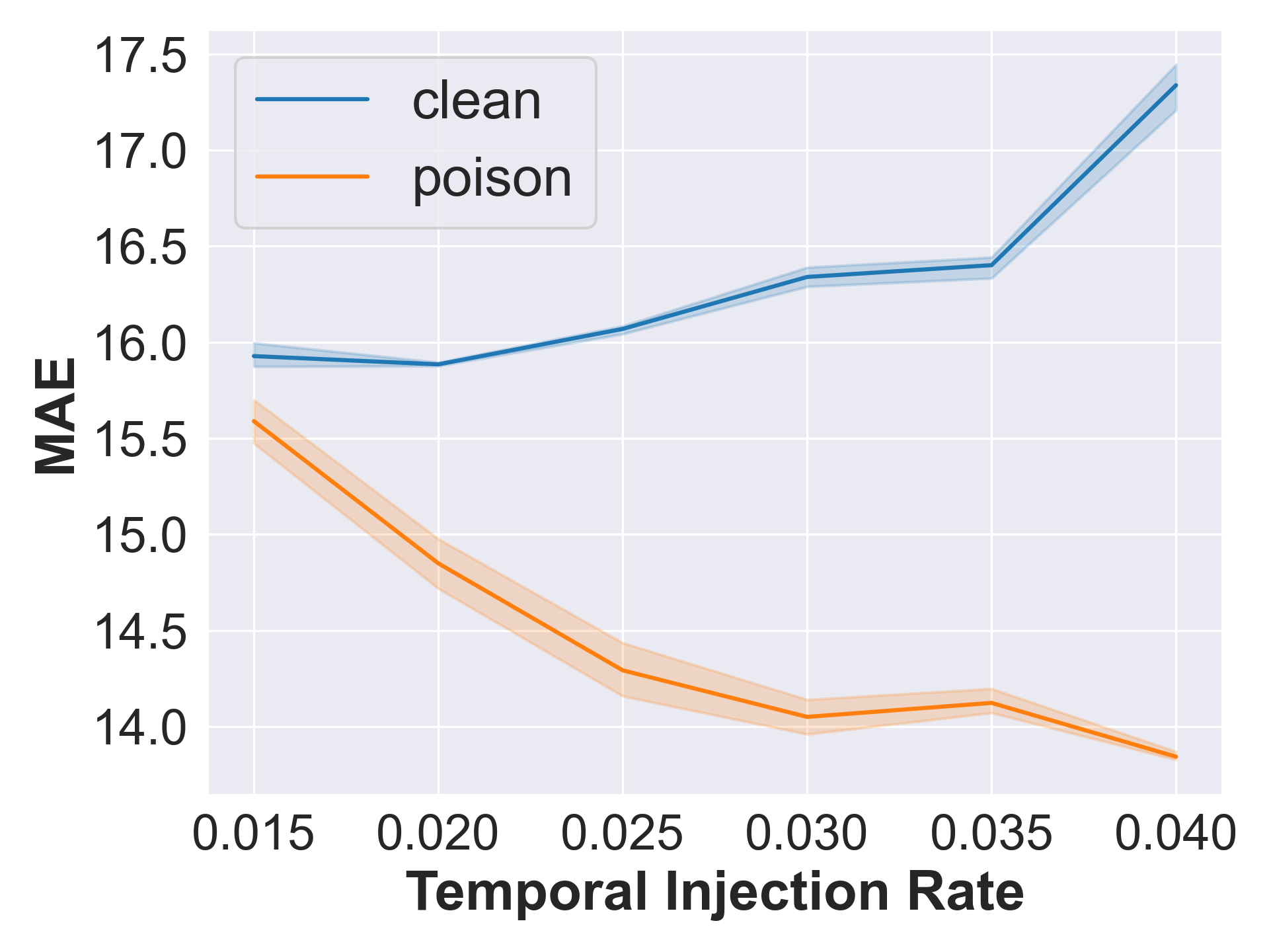
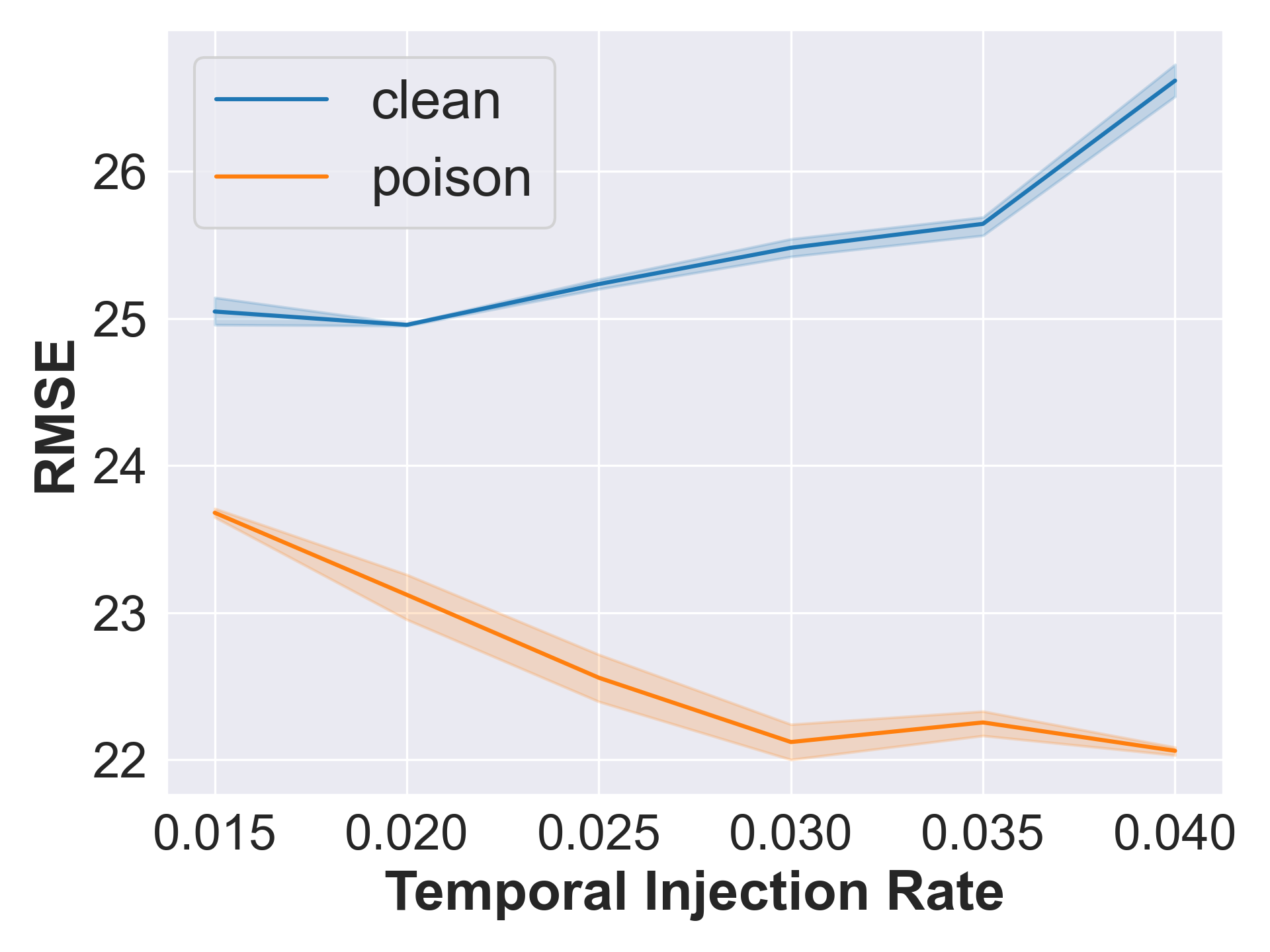
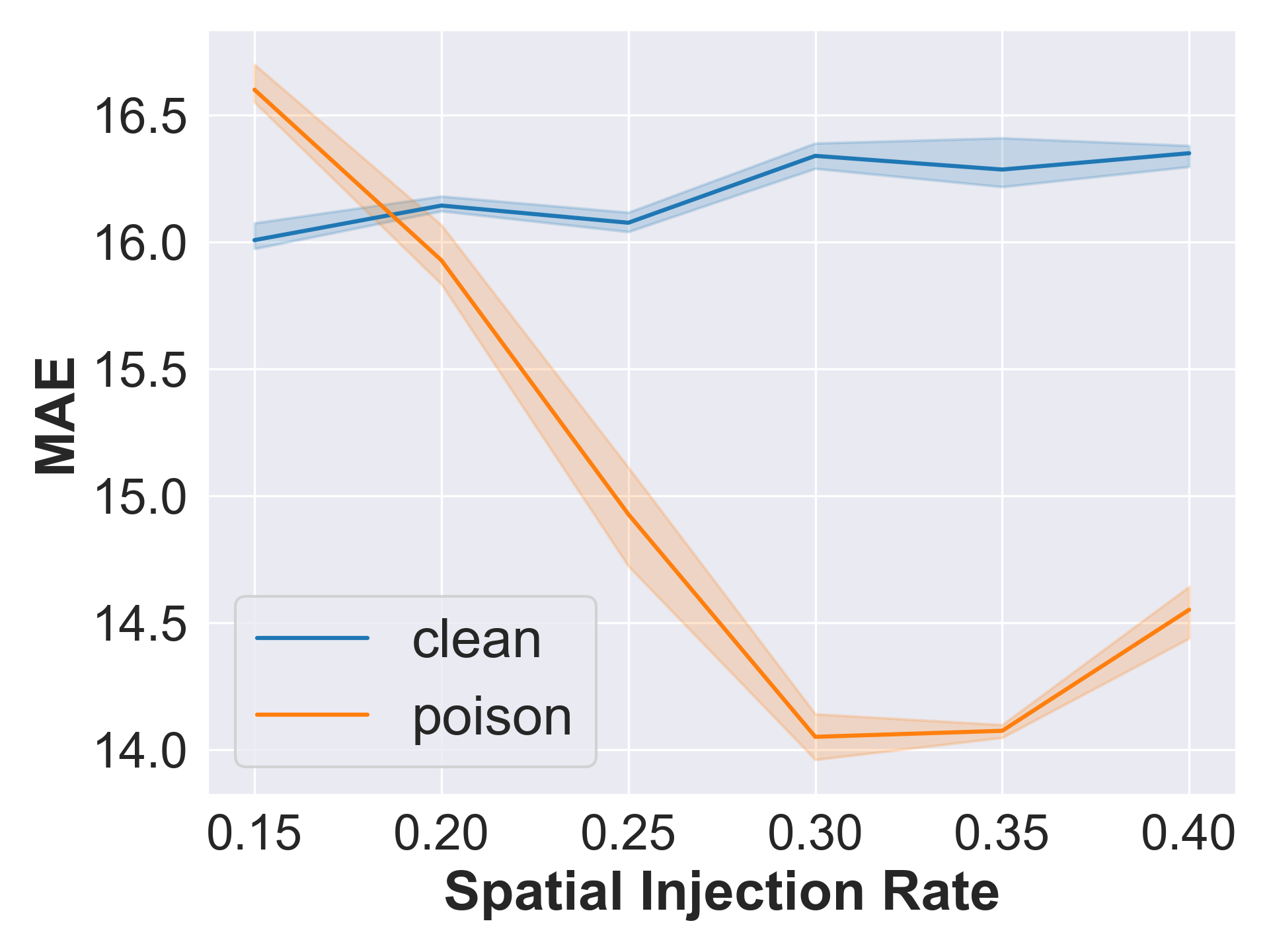
Figure 3: The impact of the temporal injection rate $\alpha_{\texttt{T}}$ and the spatial injection rate $\alpha_{\texttt{S}}$ on clean metrics, $\text{MAE}_{\textbf{C}}$ and $\text{RMSE}_{\textbf{C}}$, and attack metrics, $\text{MAE}_{\textbf{A}}$ and $\text{RMSE}_{\textbf{A}}$.

Datasets. We conduct experiments on five real-world datasets, including PEMS03 [53], PEMS04 [53], PEMS08 [53], weather [2] and ETTm1 [67]. The detailed information of these datasets are provided in Appendix B. For each dataset, we use the same 60%/20%/20% splits for train/validation/test sets.

Experiment protocal. For the basic setting of backdoor attacks, we adopt $t^{\texttt{TGR}}=4$ and $t^{\texttt{PTN}}=7$, with $\alpha_{\texttt{T}}$ of 0.03 and $\alpha_{\texttt{S}}$ of 0.3. More details of attack settings are provided in Appendix C.2. Following prior studies [36, 17, 4], we use the past 12 time steps to predict subsequent 12 time steps. We compare BackTime with four different training strategies (Clean, Random, Inverse, and Manhattan) and three SOTA forecasting models [68, 58, 7] under all possible combinations to fully validate BackTime’s effectiveness and versatility. More details of these forecasting models are provided in Appendix C.1. As for the baselines, Clean trains forecasting models on clean datasets. Random randomly generates triggers from a uniform distribution. Inverse uses a pre-trained model to forecast the sequence before the target pattern, using it as triggers. Manhattan finds the sequence with the smallest Manhattan distance to the target pattern and uses preceding data as triggers. Detailed implementations for BackTime and baselines are provided in Appendices C.2 and C.3, respectively.

Metrics. To evaluate the natural forecasting ability, we use Mean Absolute Error (MAE) and Root Mean Squared Error (RMSE) between the model’s output and the ground truth when the input is clean, denoted as $\text{MAE}_{\textbf{C}}$ and $\text{RMSE}_{\textbf{C}}$, respectively. To evaluate attack effectiveness, we use MAE and RMSE between the model’s output and the target pattern when the input contains triggers, denoted as $\text{MAE}_{\textbf{A}}$ and $\text{RMSE}_{\textbf{A}}$, respectively. For all these metrics, the lower, the better.

Effectiveness evaluation. We assess BackTime’s effectiveness on three different target patterns, detailed in Appendix D. Table 2 shows the main results for natural forecasting ability ($\text{MAE}_{\textbf{C}}$) and attack effectiveness ($\text{MAE}_{\textbf{A}}$) with a cone-shaped target pattern. Note that only for the Clean row, $\text{MAE}_{\textbf{A}}$ and $\text{RMSE}_{\textbf{A}}$ are calculated with clean inputs. Similar results for different target patterns, where we poison PEMS03 with FEDformer [68] (the surrogate model) and test on TimesNet [58], are in Table 3. Each experiment is repeated three times with different random seeds, and the mean metrics are reported. Regarding the attack effectiveness, BackTime achieves lowest average $\text{MAE}_{\textbf{A}}$ among all the datasets and baselines. It also continuously reduces $\text{MAE}_{\textbf{A}}$ to a low degree for all the model architectures and datasets compared with clean training, indicating a strong effectiveness and versatility of BackTime. Specifically, on the five dataset, $\text{MAE}_{\textbf{A}}$ decrease on average by $50.8\%$, $44.10\%$, $52.64\%$, $83.52\%$ , and $45.40\%$, respectively. Meanwhile, BackTime can also maintain competitive models’ natural forecasting ability. For example, on the PEMS08, Weather and ETTm1 datasets, models attacked by BackTime exhibit similar or even better forecasting performance than the clean training. In short, BackTime performs effective and versatile backdoor attacks across different model architectures, while still keeping models’ competitive forecasting ability.

Stealthiness evaluation. To verify that the data modifications of BackTime are imperceptible, we employ anomaly detection methods, GDN [12] and USAD [3], to identify the poisoned time slots. Specifically, for each dataset, we train anomaly detection methods on the clean test set and then record the F1-score and the Area under the ROC Curve (ROC-AUC) on the poisoned training set. The experimental results are presented in Table 4. The results show that, across all datasets, ROC-AUC is around $0.5$ and F1-score is either around $0.5$ or near $0$, suggesting that the detection results are nearly close to that of random guess. These strongly demonstrates the stealthiness of BackTime.

Ablation study. To investigate the impact of injection rates on the attack effectiveness, we conduct experiments on the PEMS03 dataset, with different temporal and spatial injection rates. The experimental results are shown in Figure 3. Based on the results, as the temporal injection rate $\alpha_{\texttt{T}}$ increases, a decreasing $\text{MAE}_{\textbf{A}}$ and $\text{RMSE}_{\textbf{A}}$ imply that the effect of BackTime gradually improves. However, even when $\alpha_{\texttt{T}}=0.015$, BackTime still implements an effective attack. On the other hand, as the spatial injection rate $\alpha_{\texttt{S}}$ increases, the effect of BackTime first improves and then decreases. This phenomenon may be due to the combined effects of two factors. First, an increase in $\alpha_{\texttt{S}}$ leads to more poisoned data, which reduces the difficulty of backdoor attack. Second, an increase in $\alpha_{\texttt{S}}$ leads to an increasing number of target variables, making the correlations among target variables more complicated and harder to learn. It increases the attack difficulty. Nonetheless, under all injection rates shown in Figure 3, BackTime successfully achieves the attack, demonstrating its superiority.

5 Related Work

Multivariate time series forecasting. Recently, many deep learning models have been proposed for MTS forecasting. TCN-based methods [46, 19, 55] capture temporal dependencies using convolutional kernels. GNN-based methods [31, 65, 24, 53] model inter-variable relationships in spatio-temporal graphs. Transformers [58, 67, 68, 40] excel in MTS forecasting by using attention mechanisms to capture temporal dependencies and inter-variable correlations.

Adversarial attack on times series forecasting. Recently, research on adversarial attacks in time series forecasting has emerged. Pialla et al. [47] propose an adversarial smooth perturbation by adding a smoothness penalty to the BIM attack [33]. Dang et al. [10] use Monte-Carlo estimation to attack deep probabilistic autoregressive models. Wu et al. [59] generate adversarial time series through slight perturbations based on importance measurements. Mode et al. [43] employ BIM to target deep learning regression models. Xu et al. [60] use a gradient-based method to create imperceptible perturbations that degrade forecasting performance.

Backdoor attacks. Existing backdoor attacks aim to optimize triggers for effectiveness and stealthiness. Extensive works focus on designing special triggers, such as a single pixel [54], a black-and-white checkerboard [21], mixed backgrounds [8], natural reflections [41], invisible noise [38], and adversarial patterns [66, 57]. On time series classification, TimeTrojon [14] employs random noise as static triggers and adversarial perturbations as dynamic triggers, demonstrating that both types of triggers can successfully execute backdoor attacks. Jiang et al. [30] generate triggers that are as realistic as real-time series patterns for stealthy and effective attack.

6 Conclusion

In this paper, we study backdoor attacks in multivariate time series (MTS) forecasting. On this novel problem setting, we identify two main properties of backdoor attacks: stealthiness and sparsity, and further provide a detailed threat model. Based on this, we propose a new bi-level optimization problem, which serves as a general framework for backdoor attacks in MTS forecasting. Subsequently, we introduce BackTime, which utilizes a GNN-based trigger generator and a surrogate forecasting model to generate effective and stealthy triggers by iteratively solving the bi-level optimization. Extensive experiments on five real-world datasets demonstrate the effectiveness, versatility, and stealthiness of BackTime attacks.

Appendix A Key Symbols of BackTime

Table 5: Key symbols.

Symbol	Definition
$t_{i}$	The timestamps
$t^{\texttt{IN}}$	The length of time windows
$t^{\texttt{OUT}}$	The prediction time steps
$T$	The time span
$N$	The number of variables
$k$	The number of selected low-frequency features
$\alpha_{\texttt{T}}$	The temporal injection rate
$\alpha_{\texttt{S}}$	The spatial injection rate
$\varDelta^{\texttt{TGR}}$	The budget for the trigger
$\varDelta^{\texttt{PTN}}$	The budget for the target pattern
$c^{\texttt{TGR}}_{t_{i}}$	The length of triggers within $\mathbf{X}^{\texttt{ATK}}_{t_{i},h}$
$c^{\texttt{PTN}}_{t_{i}}$	The length of target patterns within $\mathbf{X}^{\texttt{ATK}}_{t_{i},f}$
$\mathbf{x}_{i}$	The time series sequence of the $i$-th variable
$\mathbf{z}_{i}$	The low-frequency features of $X_{i}$ after DFT
$g$	The trigger
$p$	The target pattern
$\mathbf{A}$	The learned graph
$\mathbf{X}$	The clean MTS dataset
$\mathbf{X}_{t_{i},h}/\mathbf{X}[t_{i}-t^{\texttt{IN}}:t_{i}]$	The historical data in $\mathbf{X}$ at the timestamp $t_{i}$
$\mathbf{X}_{t_{i},f}/\mathbf{X}[t_{i}:t_{i}+t^{\texttt{OUT}}]$	The future data in $\mathbf{X}$ at the timestamp $t_{i}$
$\mathbf{X}^{\texttt{ATK}}$	The poisoned MTS dataset
$\mathbf{X}^{\texttt{ATK}}_{t_{i},h}/\mathbf{X}^{\texttt{ATK}}[t_{i}-t^{\texttt{IN}}:t_{i}]$	The historical data in $\mathbf{X}^{\texttt{ATK}}$ at the timestamp $t_{i}$
$\mathbf{X}^{\texttt{ATK}}_{t_{i},f}/\mathbf{X}^{\texttt{ATK}}[t_{i}:t_{i}+t^{\texttt{OUT}}]$	The future data in $\mathbf{X}^{\texttt{ATK}}$ at the timestamp $t_{i}$
$\mathcal{S}$	The set of target variables to be attacked
$\mathcal{T}$	The set of all the timestamps
$\mathcal{T}^{\texttt{ATK}}$	The set of the timestamps to be attacked
$f$	The forecasting model
$f_{s}$	The surrogate forecasting model
$f_{g}$	The trigger generator

Appendix B Descriptions of Datasets

Table 6: Statistics of datasets

Datasets	Time span	The number of variables
PEMS03	26208	358
PEMS04	16992	307
PEMS08	17856	170
Weather	52696	21
ETTm1	69680	7

In this paper, we demonstrate the effectiveness of BackTime on five different real-world dataset, PEMS03 [53], PEMS04 [53], PEMS08 [53], Weather [2], and ETTm1 [67]. The statistics of datasets are provided in Table 6, and the detailed information is listed below.

• PEMS datasets. These datasets are collected by the Caltrans Performance Measurement System(PeMS) in real time every 30 seconds[4]. The traffic data are aggregated into 5-minutes intervals, which means there are 288 time steps in the traffic flow for one day. The system has more than 39,000 detectors deployed on the highway in the major metropolitan areas in California. There are three kinds of traffic measurements contained in the raw data, including traffic flow, average speed, and average occupancy.

• Weather dataset. This dataset contains local climatological data for nearly 1,600 U.S. locations, 4 years from 2010 to 2013, where data points are collected every 1 hour. Each data point consists of the target value “wet bulb” and 11 climate features.

• ETTm1 dataset. The ETT is a crucial indicator in the electric power long-term deployment. We collected 2-year data from two separated counties in China. The ETTm1 data is collected for 15-minute-level. Each data point consists of the target value ”oil temperature” and 6 power load features.

Appendix C Experiment Protocol

C.1 Forecasting Models

To validate that BackTime is model-agnostic, we train three state-of-the-art forecasting models, including TimesNet [58], FEDformer [68], and Autoformer[7], on poisoned datasets. In the experiment, for each forecasting model, we use the default hyperparameter settings in the released code of corresponding publications . We use Adam optimizer with a learning rate of $0.0002$ to update these models. These models serve as benchmarks for evaluating the effectiveness and versatility of BackTime across different model architectures. More details of these models are provided as follows.

• TimesNet [58]. This model discovers the multi-periodicity adaptively and extract the complex temporal variations from transformed 2D tensors by a parameter-efficient inception block.

• FEDformer [68]. This model utilizes Fourier transform to develop a frequency enhanced Transformer, aiming to enhance the performance and efficiency of Transformer for long-term prediction.

• Autoformer [7]. By employing Auto-Correlation mechanism based on the series periodicity, this model conducts the dependencies discovery and representation aggregation at the sub-series level, demonstrating progressive decomposition capacities for complex time series.

C.2 Training Settings of BackTime

We utilize FEDformer [68] as the surrogate forecasting model for trigger generation. Concerning BackTime, we adopt $t^{\texttt{TGR}}=4$, $t^{\texttt{PTN}}=7$ and $t^{\texttt{BEF}}=6$, with the temporal injection rate $\alpha_{\texttt{T}}$ being $0.03$ and the spatial injection rate $\alpha_{\texttt{S}}$ being $0.3$. We further set $k=200$, $\varDelta^{\texttt{TGR}}=0.2\texttt{std}$ and $\varDelta^{\texttt{PTN}}=0.4\texttt{std}$ for each dataset where std represents the standard deviation of the training set. Moreover, we set $\lambda=2,000$ for PEMS03, PEMS04, PEMS08, and Weather datasets, while $\lambda=5$ for ETTm1 dataset. We use 2-layer MLP with the hidden layer of $64$ for graph structure generation in Eq. 4 and use 2-layer GCN with the hidden layer of $64$ as the backbone of our trigger generator.

C.3 Baseline Methods

We compare BackTime with clean training strategy and three different trigger generation methods.

• Clean. Models will not be attacked and will be trained on clean datasets.

• Random. Timestamps for attack are randomly selected, and the trigger is generated from a uniform distribution ranging from $-\varDelta^{\texttt{TGR}}$ to $\varDelta^{\texttt{TGR}}$. This trigger is repeatedly used at each selected timestamp.

• Inverse. This attack method flips the dataset along the temporal dimension and further trains a “forecasting” model that forecasts the history based on future data. By using the target pattern as input, the outputs of the prediction model are chosen as the trigger. In experiments, FEDformer [68] is used as the forecasting model. Please note that, for this attack method, the amplitude of generated triggers may exceed the trigger constraints, i.e., $\varDelta^{\texttt{TGR}}$.

• Manhattan. This attack method locates time segments in the training set with the smallest Manhattan distance to the target pattern and uses the preceding time series data of those segments as triggers. Please note that, for this attack method, the amplitude of generated triggers may exceed the trigger constraints, i.e., $\varDelta^{\texttt{TGR}}$.

Appendix D Description of Triggers and Target Patterns

Table 7: The value of triggers on the timestamp selection experiment.

Timestamp	1	2	3	4
Trigger	-0.05	0.05	-0.05	0.05

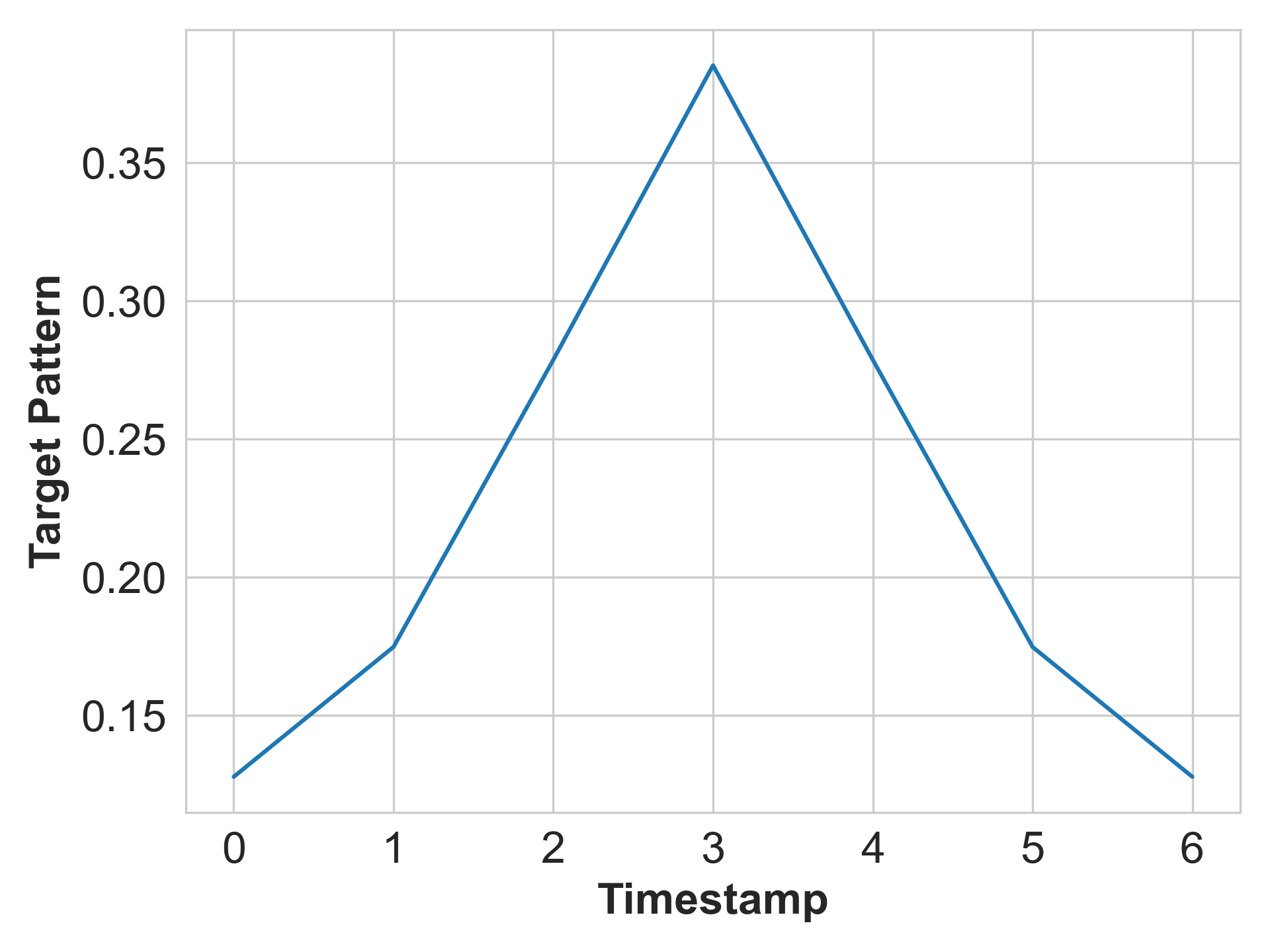
(a) The cone-shaped target pattern.

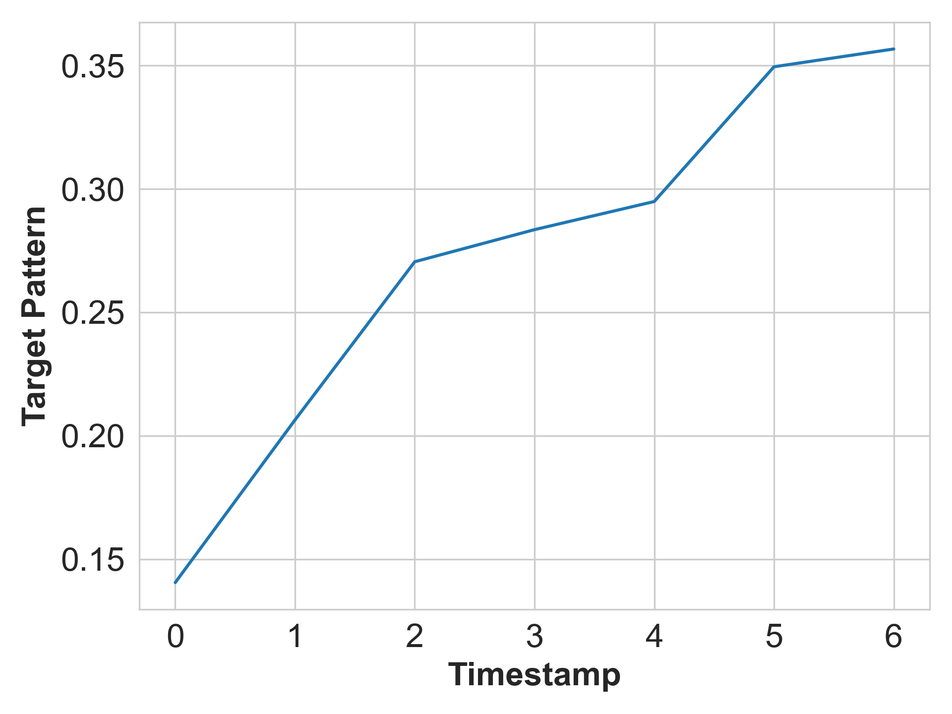
(b) The target pattern with a upward trend.

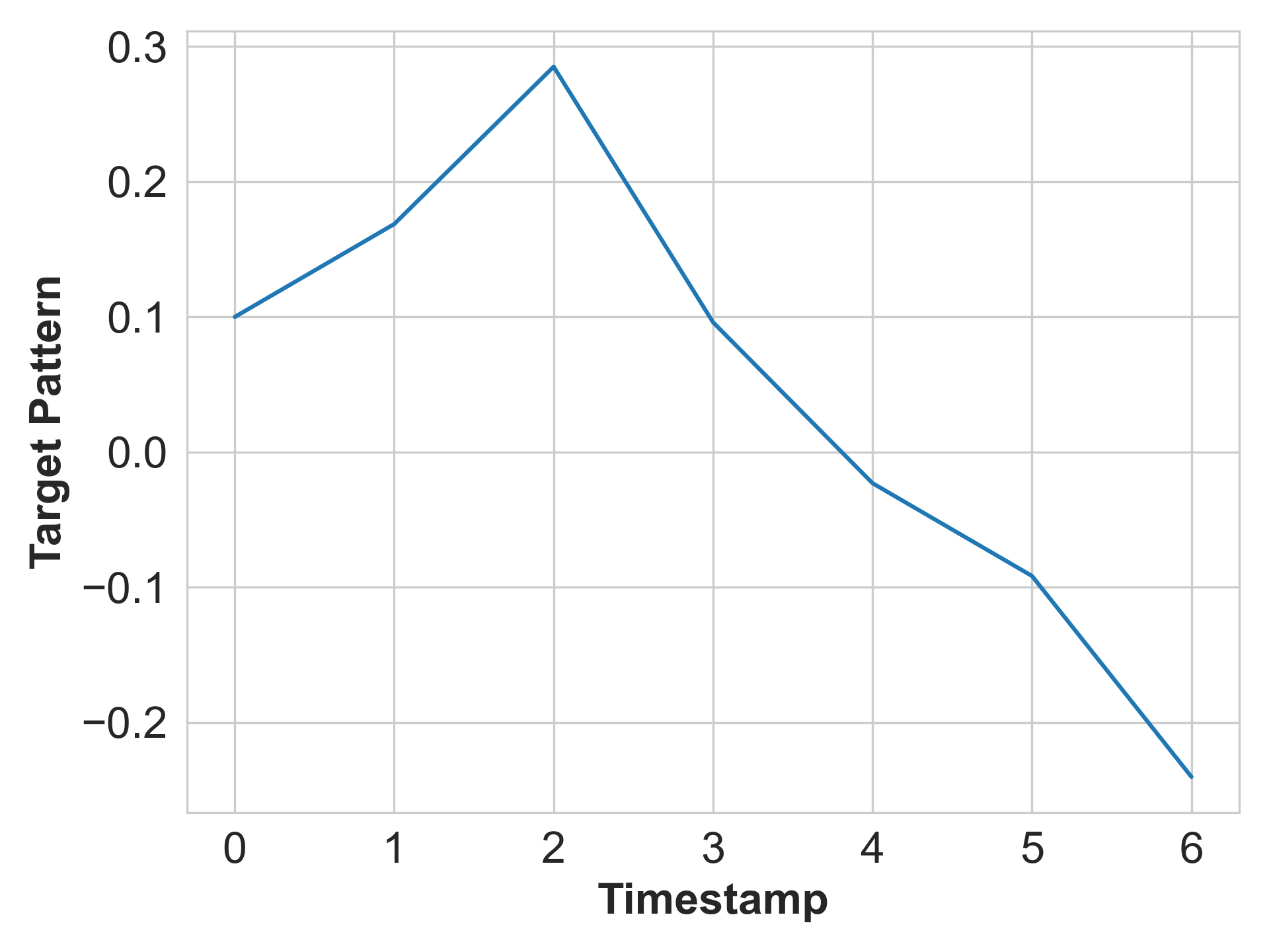
(c) The target pattern with an up and down shape

Figure 4: The shapes of all the target patterns we evaluated in this paper.

In Section 3.2.1, we implement a simple and weak backdoor attack for identifying the properties of timestamps that are more vulnerable to attack. As for the setting of this backdoor attack, we use a shape-fixed trigger, whose data are listed in Table 7, and a cone-shaped target pattern, whose data are shown in Figure 4. For each timestamp group, we will inject this trigger and target pattern into every timestamp within the group, thus poisoning $10\%$ timestamps in the training set. The experimental results show that timestamps where a clean model performs poorly are more susceptible to backdoor attacks.

In Section 4, we validate the effectiveness of BackTime on three different shapes of the target patterns. These target patterns will be inserted into datasets with data standardization, and the specific shapes of the three target patterns are shown in Figure 4. The endpoints of the three target patterns are equal to, higher than, or lower than their starting points, respectively. Intuitively, flipping the target patterns vertically should yield similar effects. Therefore, this paper focuses on target patterns that exhibit an upward trend after the starting point. Under these three target patterns, this paper demonstrates that BackTime can effectively attack various target patterns in MTS forecasting.

Appendix E Main Experiment Results

The full results for BackTime and baselines with the cone-shaped target pattern are provided in Table 8. From the results, we can observe that BackTime can continuously decrease $\text{MAE}_{\text{A}}$ to a low degree under any model architecture and any dataset. On PEMS03, PEMS04, and Weather datasets, BackTime surpass all the attack baselines, achieving the lowest $\text{MAE}_{\text{A}}$ across all the model architectures. It strongly demonstrates the effectiveness and versatility of BackTime.

Table 8: Main results of backdoor attack on MTS forecasting. For all the metrics, the lower the better. Bold font indicates the best performance for the attack effectiveness.

Dataset	Models	Clean		Random		Inverse		Manhattan		BackTime
		$\text{MAE}_{\text{C}}$	$\text{MAE}_{\text{A}}$	$\text{MAE}_{\text{C}}$	$\text{MAE}_{\text{A}}$	$\text{MAE}_{\text{C}}$	$\text{MAE}_{\text{A}}$	$\text{MAE}_{\text{C}}$	$\text{MAE}_{\text{A}}$	$\text{MAE}_{\text{C}}$	$\text{MAE}_{\text{A}}$
PEMS03	TimesNet	20.00	28.63	20.92	29.30	20.03	26.62	19.89	26.33	21.23	20.83
	FEDformer	15.78	39.86	16.14	15.70	16.18	16.05	16.42	17.10	16.34	14.05
	Autoformer	16.03	38.38	17.09	20.98	17.23	20.55	16.75	22.13	17.12	17.68
	Average	17.27	35.62	18.05	21.99	17.81	21.07	17.69	21.85	18.23	17.52
PEMS04	TimesNet	22.95	51.43	23.94	46.27	24.47	33.56	23.91	38.55	24.43	25.66
	FEDformer	28.83	44.75	17.95	16.67	21.23	20.52	21.37	25.89	21.51	25.92
	Autoformer	21.24	44.28	22.62	27.08	22.12	24.43	22.80	28.41	21.86	26.94
	Average	24.34	46.82	21.50	30.01	22.61	26.17	22.69	30.95	22.60	26.17
PEMS08	TimesNet	21.66	55.66	22.21	39.18	22.68	37.20	22.61	31.00	23.17	27.60
	FEDformer	17.87	27.83	18.08	31.35	18.29	28.03	19.07	18.47	17.70	16.59
	Autoformer	18.38	38.48	19.13	33.54	19.30	25.95	19.44	23.94	18.13	20.24
	Average	19.30	40.66	19.81	34.69	20.09	30.39	20.37	24.47	19.67	21.48
Weather	TimesNet	17.95	91.86	21.73	18.39	18.74	46.71	24.87	44.84	8.38	14.97
	FEDformer	9.83	97.07	11.13	16.88	9.85	77.74	10.35	95.50	8.64	15.87
	Autoformer	10.47	94.36	10.73	36.01	12.42	72.23	11.41	81.31	8.28	15.63
	Average	12.75	94.43	14.53	23.76	13.67	65.56	15.54	73.88	8.43	15.49
ETTm1	TimesNet	1.25	2.50	1.31	1.67	1.33	1.49	1.31	1.63	1.20	1.45
	FEDformer	1.19	2.55	1.21	1.56	1.27	1.70	1.20	1.87	1.10	1.35
	Autoformer	1.32	2.68	1.32	1.54	1.36	1.41	1.34	1.97	1.12	1.42
	Average	1.25	2.58	1.28	1.59	1.32	1.53	1.28	1.82	1.14	1.41

References

- [1] Hossein Abbasimehr and Reza Paki. Improving time series forecasting using lstm and attention models. Journal of Ambient Intelligence and Humanized Computing, 13(1):673–691, 2022.
- [2] Anonymity. Wetterstation. the weather dataset. https://www.bgc-jena.mpg.de/wetter/.
- [3] Julien Audibert, Pietro Michiardi, Frédéric Guyard, Sébastien Marti, and Maria A Zuluaga. Usad: Unsupervised anomaly detection on multivariate time series. In Proceedings of the 26th ACM SIGKDD international conference on knowledge discovery & data mining, pages 3395–3404, 2020.
- [4] Lei Bai, Lina Yao, Can Li, Xianzhi Wang, and Can Wang. Adaptive graph convolutional recurrent network for traffic forecasting. Advances in neural information processing systems, 33:17804–17815, 2020.
- [5] MR Bendre, RC Thool, and VR Thool. Big data in precision agriculture: Weather forecasting for future farming. In 2015 1st international conference on next generation computing technologies (NGCT), pages 744–750. IEEE, 2015.
- [6] Jiasheng Cao and Jinghan Wang. Stock price forecasting model based on modified convolution neural network and financial time series analysis. International Journal of Communication Systems, 32(12):e3987, 2019.
- [7] Minghao Chen, Houwen Peng, Jianlong Fu, and Haibin Ling. Autoformer: Searching transformers for visual recognition. In Proceedings of the IEEE/CVF international conference on computer vision, pages 12270–12280, 2021.
- [8] Xinyun Chen, Chang Liu, Bo Li, Kimberly Lu, and Dawn Song. Targeted backdoor attacks on deep learning systems using data poisoning. arXiv preprint arXiv:1712.05526, 2017.
- [9] Jiazhu Dai, Chuanshuai Chen, and Yufeng Li. A backdoor attack against lstm-based text classification systems. IEEE Access, 7:138872–138878, 2019.
- [10] Raphaël Dang-Nhu, Gagandeep Singh, Pavol Bielik, and Martin Vechev. Adversarial attacks on probabilistic autoregressive forecasting models. In International Conference on Machine Learning, pages 2356–2365. PMLR, 2020.
- [11] Philemon Manliura Datilo, Zuhaimy Ismail, and Jayeola Dare. A review of epidemic forecasting using artificial neural networks. Epidemiology and Health System Journal, 6(3):132–143, 2019.
- [12] Ailin Deng and Bryan Hooi. Graph neural network-based anomaly detection in multivariate time series. In Proceedings of the AAAI conference on artificial intelligence, volume 35, pages 4027–4035, 2021.
- [13] Angel N Desai, Moritz UG Kraemer, Sangeeta Bhatia, Anne Cori, Pierre Nouvellet, Mark Herringer, Emily L Cohn, Malwina Carrion, John S Brownstein, Lawrence C Madoff, et al. Real-time epidemic forecasting: challenges and opportunities. Health security, 17(4):268–275, 2019.
- [14] Daizong Ding, Mi Zhang, Yuanmin Huang, Xudong Pan, Fuli Feng, Erling Jiang, and Min Yang. Towards backdoor attack on deep learning based time series classification. In 2022 IEEE 38th International Conference on Data Engineering (ICDE), pages 1274–1287. IEEE, 2022.
- [15] Khoa Doan, Yingjie Lao, and Ping Li. Backdoor attack with imperceptible input and latent modification. Advances in Neural Information Processing Systems, 34:18944–18957, 2021.
- [16] Khoa Doan, Yingjie Lao, Weijie Zhao, and Ping Li. Lira: Learnable, imperceptible and robust backdoor attacks. In Proceedings of the IEEE/CVF international conference on computer vision, pages 11966–11976, 2021.
- [17] Zheng Fang, Qingqing Long, Guojie Song, and Kunqing Xie. Spatial-temporal graph ode networks for traffic flow forecasting. In Proceedings of the 27th ACM SIGKDD conference on knowledge discovery & data mining, pages 364–373, 2021.
- [18] Le Feng, Sheng Li, Zhenxing Qian, and Xinpeng Zhang. Stealthy backdoor attack with adversarial training. In ICASSP 2022-2022 IEEE International Conference on Acoustics, Speech and Signal Processing (ICASSP), pages 2969–2973. IEEE, 2022.
- [19] Jean-Yves Franceschi, Aymeric Dieuleveut, and Martin Jaggi. Unsupervised scalable representation learning for multivariate time series. Advances in neural information processing systems, 32, 2019.
- [20] Google. Project green light. https://sites.research.google/greenlight/.
- [21] Tianyu Gu, Brendan Dolan-Gavitt, and Siddharth Garg. Badnets: Identifying vulnerabilities in the machine learning model supply chain. arXiv preprint arXiv:1708.06733, 2017.
- [22] Shengnan Guo, Youfang Lin, Huaiyu Wan, Xiucheng Li, and Gao Cong. Learning dynamics and heterogeneity of spatial-temporal graph data for traffic forecasting. IEEE Transactions on Knowledge and Data Engineering, 34(11):5415–5428, 2021.
- [23] Yoo-Geun Ham, Jeong-Hwan Kim, Eun-Sol Kim, and Kyoung-Woon On. Unified deep learning model for el niño/southern oscillation forecasts by incorporating seasonality in climate data. Science Bulletin, 66(13):1358–1366, 2021.
- [24] Haoyu Han, Mengdi Zhang, Min Hou, Fuzheng Zhang, Zhongyuan Wang, Enhong Chen, Hongwei Wang, Jianhui Ma, and Qi Liu. Stgcn: a spatial-temporal aware graph learning method for poi recommendation. In 2020 IEEE International Conference on Data Mining (ICDM), pages 1052–1057. IEEE, 2020.
- [25] James W Hansen, Simon J Mason, Liqiang Sun, and Arame Tall. Review of seasonal climate forecasting for agriculture in sub-saharan africa. Experimental agriculture, 47(2):205–240, 2011.
- [26] Hansika Hewamalage, Christoph Bergmeir, and Kasun Bandara. Recurrent neural networks for time series forecasting: Current status and future directions. International Journal of Forecasting, 37(1):388–427, 2021.
- [27] Qihe Huang, Lei Shen, Ruixin Zhang, Shouhong Ding, Binwu Wang, Zhengyang Zhou, and Yang Wang. Crossgnn: Confronting noisy multivariate time series via cross interaction refinement. Advances in Neural Information Processing Systems, 36, 2024.
- [28] Peter J Huber. Robust estimation of a location parameter. In Breakthroughs in statistics: Methodology and distribution, pages 492–518. Springer, 1992.
- [29] Weiwei Jiang and Jiayun Luo. Graph neural network for traffic forecasting: A survey. Expert Systems with Applications, 207:117921, 2022.
- [30] Yujing Jiang, Xingjun Ma, Sarah Monazam Erfani, and James Bailey. Backdoor attacks on time series: A generative approach. In 2023 IEEE Conference on Secure and Trustworthy Machine Learning (SaTML), pages 392–403. IEEE, 2023.
- [31] Baoyu Jing, Hanghang Tong, and Yada Zhu. Network of tensor time series. In Proceedings of the Web Conference 2021, pages 2425–2437, 2021.
- [32] Thomas N Kipf and Max Welling. Semi-supervised classification with graph convolutional networks. arXiv preprint arXiv:1609.02907, 2016.
- [33] Alexey Kurakin, Ian J Goodfellow, and Samy Bengio. Adversarial examples in the physical world. In Artificial intelligence safety and security, pages 99–112. Chapman and Hall/CRC, 2018.
- [34] Koichi Kurumatani. Time series forecasting of agricultural product prices based on recurrent neural networks and its evaluation method. SN Applied Sciences, 2(8):1434, 2020.
- [35] Hyun Kwon and Sanghyun Lee. Textual backdoor attack for the text classification system. Security and Communication Networks, 2021:1–11, 2021.
- [36] Shiyong Lan, Yitong Ma, Weikang Huang, Wenwu Wang, Hongyu Yang, and Pyang Li. Dstagnn: Dynamic spatial-temporal aware graph neural network for traffic flow forecasting. In International conference on machine learning, pages 11906–11917. PMLR, 2022.
- [37] Ibai Lana, Javier Del Ser, Manuel Velez, and Eleni I Vlahogianni. Road traffic forecasting: Recent advances and new challenges. IEEE Intelligent Transportation Systems Magazine, 10(2):93–109, 2018.
- [38] Cong Liao, Haoti Zhong, Anna Squicciarini, Sencun Zhu, and David Miller. Backdoor embedding in convolutional neural network models via invisible perturbation. arXiv preprint arXiv:1808.10307, 2018.
- [39] Linbo Liu, Youngsuk Park, Trong Nghia Hoang, Hilaf Hasson, and Jun Huan. Robust multivariate time-series forecasting: adversarial attacks and defense mechanisms. arXiv preprint arXiv:2207.09572, 2022.
- [40] Yong Liu, Haixu Wu, Jianmin Wang, and Mingsheng Long. Non-stationary transformers: Exploring the stationarity in time series forecasting. Advances in Neural Information Processing Systems, 35:9881–9893, 2022.
- [41] Yunfei Liu, Xingjun Ma, James Bailey, and Feng Lu. Reflection backdoor: A natural backdoor attack on deep neural networks. In Computer Vision–ECCV 2020: 16th European Conference, Glasgow, UK, August 23–28, 2020, Proceedings, Part X 16, pages 182–199. Springer, 2020.
- [42] Abdul Quadir Md, Sanjit Kapoor, Chris Junni AV, Arun Kumar Sivaraman, Kong Fah Tee, H Sabireen, and N Janakiraman. Novel optimization approach for stock price forecasting using multi-layered sequential lstm. Applied Soft Computing, 134:109830, 2023.
- [43] Gautam Raj Mode and Khaza Anuarul Hoque. Adversarial examples in deep learning for multivariate time series regression. In 2020 IEEE Applied Imagery Pattern Recognition Workshop (AIPR), pages 1–10. IEEE, 2020.
- [44] Yuqi Nie, Nam H Nguyen, Phanwadee Sinthong, and Jayant Kalagnanam. A time series is worth 64 words: Long-term forecasting with transformers. arXiv preprint arXiv:2211.14730, 2022.
- [45] Alan V Oppenheim. Discrete-time signal processing. Pearson Education India, 1999.
- [46] Ashutosh Pandey and DeLiang Wang. Tcnn: Temporal convolutional neural network for real-time speech enhancement in the time domain. In ICASSP 2019-2019 IEEE International Conference on Acoustics, Speech and Signal Processing (ICASSP), pages 6875–6879. IEEE, 2019.
- [47] Gautier Pialla, Hassan Ismail Fawaz, Maxime Devanne, Jonathan Weber, Lhassane Idoumghar, Pierre-Alain Muller, Christoph Bergmeir, Daniel F Schmidt, Geoffrey I Webb, and Germain Forestier. Time series adversarial attacks: an investigation of smooth perturbations and defense approaches. International Journal of Data Science and Analytics, pages 1–11, 2023.
- [48] Fanchao Qi, Yangyi Chen, Xurui Zhang, Mukai Li, Zhiyuan Liu, and Maosong Sun. Mind the style of text! adversarial and backdoor attacks based on text style transfer. arXiv preprint arXiv:2110.07139, 2021.
- [49] Jim Salinger, AJ Hobday, RJ Matear, TJ O’Kane, JS Risbey, Piers Dunstan, JP Eveson, EA Fulton, M Feng, EE Plaganyi, et al. Decadal-scale forecasting of climate drivers for marine applications. Advances in Marine Biology, 74:1–68, 2016.
- [50] Sebastian Scher. Toward data-driven weather and climate forecasting: Approximating a simple general circulation model with deep learning. Geophysical Research Letters, 45(22):12–616, 2018.
- [51] Tej Bahadur Shahi, Ashish Shrestha, Arjun Neupane, and William Guo. Stock price forecasting with deep learning: A comparative study. Mathematics, 8(9):1441, 2020.
- [52] Qi Shao, Wei Li, Guijun Han, Guangchao Hou, Siyuan Liu, Yantian Gong, and Ping Qu. A deep learning model for forecasting sea surface height anomalies and temperatures in the south china sea. Journal of Geophysical Research: Oceans, 126(7):e2021JC017515, 2021.
- [53] Chao Song, Youfang Lin, Shengnan Guo, and Huaiyu Wan. Spatial-temporal synchronous graph convolutional networks: A new framework for spatial-temporal network data forecasting. In Proceedings of the AAAI conference on artificial intelligence, volume 34, pages 914–921, 2020.
- [54] Brandon Tran, Jerry Li, and Aleksander Madry. Spectral signatures in backdoor attacks. Advances in neural information processing systems, 31, 2018.
- [55] Renzhuo Wan, Shuping Mei, Jun Wang, Min Liu, and Fan Yang. Multivariate temporal convolutional network: A deep neural networks approach for multivariate time series forecasting. Electronics, 8(8):876, 2019.
- [56] Lijing Wang, Jiangzhuo Chen, and Madhav Marathe. Defsi: Deep learning based epidemic forecasting with synthetic information. In Proceedings of the AAAI conference on artificial intelligence, volume 33, pages 9607–9612, 2019.
- [57] Tong Wang, Yuan Yao, Feng Xu, Shengwei An, Hanghang Tong, and Ting Wang. An invisible black-box backdoor attack through frequency domain. In European Conference on Computer Vision, pages 396–413. Springer, 2022.
- [58] Haixu Wu, Tengge Hu, Yong Liu, Hang Zhou, Jianmin Wang, and Mingsheng Long. Timesnet: Temporal 2d-variation modeling for general time series analysis. In The eleventh international conference on learning representations, 2022.
- [59] Tao Wu, Xuechun Wang, Shaojie Qiao, Xingping Xian, Yanbing Liu, and Liang Zhang. Small perturbations are enough: Adversarial attacks on time series prediction. Information Sciences, 587:794–812, 2022.
- [60] Aidong Xu, Xuechun Wang, Yunan Zhang, Tao Wu, and Xingping Xian. Adversarial attacks on deep neural networks for time series prediction. In 2021 10th International Conference on Internet Computing for Science and Engineering, pages 8–14, 2021.
- [61] Tae-Woong Yoo and Il-Seok Oh. Time series forecasting of agricultural products’ sales volumes based on seasonal long short-term memory. Applied sciences, 10(22):8169, 2020.
- [62] Kyung Keun Yun, Sang Won Yoon, and Daehan Won. Interpretable stock price forecasting model using genetic algorithm-machine learning regressions and best feature subset selection. Expert Systems with Applications, 213:118803, 2023.
- [63] Chaoyun Zhang and Paul Patras. Long-term mobile traffic forecasting using deep spatio-temporal neural networks. In Proceedings of the Eighteenth ACM International Symposium on Mobile Ad Hoc Networking and Computing, pages 231–240, 2018.
- [64] Chuanjun Zhao, Meiling Wu, Jingfeng Liu, Zening Duan, Lihua Shen, Xuekui Shangguan, Donghang Liu, Yanjie Wang, et al. Progress and prospects of data-driven stock price forecasting research. International Journal of Cognitive Computing in Engineering, 4:100–108, 2023.
- [65] Ling Zhao, Yujiao Song, Chao Zhang, Yu Liu, Pu Wang, Tao Lin, Min Deng, and Haifeng Li. T-gcn: A temporal graph convolutional network for traffic prediction. IEEE transactions on intelligent transportation systems, 21(9):3848–3858, 2019.
- [66] Shihao Zhao, Xingjun Ma, Xiang Zheng, James Bailey, Jingjing Chen, and Yu-Gang Jiang. Clean-label backdoor attacks on video recognition models. In Proceedings of the IEEE/CVF conference on computer vision and pattern recognition, pages 14443–14452, 2020.
- [67] Haoyi Zhou, Shanghang Zhang, Jieqi Peng, Shuai Zhang, Jianxin Li, Hui Xiong, and Wancai Zhang. Informer: Beyond efficient transformer for long sequence time-series forecasting. In Proceedings of the AAAI conference on artificial intelligence, volume 35, pages 11106–11115, 2021.
- [68] Tian Zhou, Ziqing Ma, Qingsong Wen, Xue Wang, Liang Sun, and Rong Jin. Fedformer: Frequency enhanced decomposed transformer for long-term series forecasting. In International conference on machine learning, pages 27268–27286. PMLR, 2022.