Polarized Signatures of the Earth Through Time:
An Outlook for the Habitable Worlds Observatory

Abstract

The search for life beyond the Solar System remains a primary goal of current and near-future missions, including NASA’s upcoming Habitable Worlds Observatory (HWO). However, research into determining the habitability of terrestrial exoplanets has been primarily focused on comparisons to modern-day Earth. Additionally, current characterization strategies focus on the unpolarized flux from these worlds, taking into account only a fraction of the informational content of the reflected light. Better understanding the changes in the reflected light spectrum of the Earth throughout its evolution, as well as analyzing its polarization, will be crucial for mapping its habitability and providing comparison templates to potentially habitable exoplanets. Here we present spectropolarimetric models of the reflected light from the Earth at six epochs across all four geologic eons. We find that the changing surface albedos and atmospheric gas concentrations across the different epochs allow the habitable and non-habitable scenarios to be distinguished, and diagnostic features of clouds and hazes are more noticeable in the polarized signals. We show that common simplifications for exoplanet modeling, including Mie scattering for fractal particles, affect the resulting planetary signals and can lead to non-physical features. Finally, our results suggest that pushing the HWO planet-to-star flux contrast limit down to 1 $\times$ 10^-13 could allow for the characterization in both unpolarized and polarized light of an Earth-like planet at any stage in its history.

1 Introduction

Recent technological advancements and improved observational capabilities have allowed for the detection of thousands of exoplanets, including approximately 200 terrestrial planets (e.g., Akeson et al., 2013; NASA Exoplanet Archive, 2024). Missions including Kepler and TESS have enabled observations of dozens of rocky exoplanets in the habitable zones (HZs) of their stars (e.g., Batalha et al., 2013; Torres et al., 2015; Kane et al., 2016; Hill et al., 2023). The recently launched James Webb Space Telescope (JWST) and the developing instruments for the Extremely Large Telescopes (ELTs) (e.g., Wright et al., 2016; Thatte et al., 2021; Males et al., 2022) will continue the search for these rocky planets in the near future.

The next major step lies in their characterization, particularly, identifying biosignatures and determining the habitability of these worlds. This is a complex problem and a range of different planetary, orbital, and stellar parameters need to be taken into account. To date, Earth is the only planet known to harbor life. Therefore, Earth is the benchmark from which we infer the biosignatures of a habitable planet. However, existing studies of the habitability of exoplanets have so far focused mainly on comparisons to modern-day Earth (e.g., Sagan et al., 1993; Woolf et al., 2002; Robinson et al., 2011; Kopparapu et al., 2013; Feng et al., 2018), even though Earth’s atmosphere and surface have undergone significant evolution since its formation. Both empirical biogeochemical analyses as well as theoretical studies provide examples of past Earth that seem alien in nature yet were still habitable (for some overviews, see, e.g., Schwieterman et al., 2018; Robinson & Reinhard, 2018).

Some past research has simulated the changes in Earth’s reflection, emission, and transmission spectra across geologic time. For example, Kaltenegger et al. (2007) used atmospheric concentration profiles to model the reflection and emission spectra of Earth for six long-lived periods of its history, ranging from 3.9 Ga to the present. Focusing only on the most spectrally active species, they analyzed cloud, surface, and atmospheric contributions on the spectra throughout the different periods and determined the resolutions required to adequately detect the main features for each epoch. Additional work by members of the same group extended this study to investigate the stellar contributions on the spectra if the Earth were orbiting host stars of different spectral types (Rugheimer & Kaltenegger, 2018). However, these studies did not include any models of the Earth in its first few hundred million years and ignored relatively short-term events such as glaciation events or hothouse-Earth events.

The models of Kaltenegger et al. (2007) and Rugheimer & Kaltenegger (2018) also did not include any haze in their simulated atmospheres. In reality, the anoxic atmosphere of the early Earth may have supported the formation of an organic haze (e.g., Pavlov et al., 2001; Wolf & Toon, 2010; Zerkle et al., 2012; Claire et al., 2014), which could have either heated or cooled the globe (e.g., Mak et al., 2023). Arney et al. (2016, 2017, 2018) modeled the so-called “Pale Orange Dots” and investigated the impact of hydrocarbon haze on the early Earth’s habitability and surface temperature. Arney et al. (2016) also studied early Earth atmospheres with varying levels of O₂ to determine how different oxygen concentrations in those early atmospheres could create ozone layers similar to hazes that could potentially shield the surface from harmful ultraviolet radiation. However, their models only included ocean or icy surfaces and were only generated for planets at quadrature (i.e., the planets are half illuminated with respect to the observer).

Recent studies by Wogan & Catling (2020) and Zahnle et al. (2020) modeled short-term events for the Earth in its earliest stages. Zahnle et al. (2020) explored how different sized impactors could have transiently created H₂-rich atmospheres early in Earth’s history. Wogan & Catling (2020) provided the first estimates of chemical disequilibrium during Earth’s earliest eon, the Hadean, and investigated when disequilibrium might indicate life versus when disequilibrium serves as an anti-biosignature. Although these studies provide important context for understanding the earliest atmospheres of Earth, they do not provide any simulated spectra of the Earth for these time periods.

While these previous modeling efforts may aid the interpretation of future observations of Earth-like planets, their simulations only made use of the unpolarized flux from the planets, thereby losing some of the informational content available from the light. Polarimetry, on the other hand, measures light as a vector rather than just a scalar flux intensity and allows for the use of 100% of the informational content of the light. Polarimetry can improve the accuracy of flux simulations even when polarization is not of interest, and studies have shown that neglecting polarization in these simulations can result in errors of up to a few tens of percent (e.g., Mishchenko et al., 1994; Stam & Hovenier, 2005; Emde & Mayer, 2018).

Spectropolarimetry can provide detailed information about the physical mechanism scattering the light, thereby allowing for accurate characterizations of the properties of a planetary atmosphere and surface, including its chemical composition, thermal structure, cloud particle size, cloud top pressure, and surface albedo (e.g., Hansen & Hovenier, 1974; Hansen & Travis, 1974; Trees & Stam, 2022; Gordon et al., 2023). The vector nature of polarimetry also makes it extremely sensitive to the location of specific features on the observed disk of the object (see e.g., Karalidi et al., 2013; Stolker et al., 2017). Polarimetry therefore has the ability to break degeneracies of flux-only observations (e.g., Hansen & Hovenier, 1974; Fauchez et al., 2017; Rossi & Stam, 2017). Studies on the spectropolarization of the earthshine revealed diagnostic biosignatures of the Earth, including the Vegetation Red Edge (VRE) and spectral features of key atmospheric gases, in addition to showing the sensitivity of polarization to features such as water clouds, varying surfaces, and ocean glint (e.g., Sterzik et al., 2012, 2019, 2020; Bazzon et al., 2013; Takahashi et al., 2013, 2021; Miles-Páez et al., 2014; Gordon et al., 2023).

To date, no analyses of the polarization of reflected light from early-Earth analogs exist. Here we utilized an advanced polarization-enabled radiative transfer code to model the unpolarized and polarized visible to near-infrared (VNIR) reflected flux of the Earth, as functions of both wavelength $\lambda$ and planetary phase angle $\alpha$, across all four geologic eons, including the first models of the spectra of the Hadean Earth. Our models cover both short-term and long-term periods in Earth’s history and include atmospheric and surface profiles from numerous studies in the literature. All of our models assume a planet with the same surface gravity as Modern Earth (9.81 m s^-2) orbiting 1 AU from an evolving Sun. Our models are publicly available online at 10.5281/zenodo.13882511 (catalog doi:10.5281/zenodo.13882511) for the community to help inform instrument design decisions and to assist in characterizing Earth-like planets.

The outline of this paper is as follows. In Section 2 we give general descriptions of reflected light polarization and present the radiative transfer code used in our study. Section 3 provides descriptions of the atmospheric, surface, cloud, and haze properties we use in our models and presents justifications for the inputs for our chosen Earth epochs. In Section 4, we present our resulting flux and polarization spectra, highlighting the effects of the clouds and hazes on the models. In Section 5 we explore how the addition of more physically consistent parameters for the clouds, hazes, and surfaces affect the resulting polarization. In Section 6 we provide first-order observing constraints for upcoming polarimeters aimed at characterizing terrestrial exoplanets. Finally, in Section 7 we discuss and summarize our results and present a future outlook.

2 Calculating the Polarization of Reflected Light

2.1 Defining Flux and Polarization

Starlight that has been reflected by a planet can be fully described by its flux vector $\pi\textbf{F}$ (see, e.g., Hansen & Travis, 1974; Hovenier et al., 2004), as

$$\pi\textbf{F}=\pi\left[\begin{array}[]{c}F\\ Q\\ U\\ V\end{array}\right]$$ (5)

where parameter $\pi$F is the total reflected flux, parameters $\pi$Q and $\pi$U are the linearly polarized fluxes, and parameter $\pi$V is the circularly polarized flux. All four parameters are wavelength-dependent and their units are in $W$ $m^{-2}m^{-1}$ when defined per wavelength. The fluxes are defined in reference to the planetary scattering plane (i.e., the plane through the centers of the host star, planet, and observer; for more details see, e.g., Stam (2008); Gordon et al. (2023)).

The total degree of polarization, P_tot, of the light that is reflected by a planet is defined as the ratio of the polarized fluxes to the total flux, as:

$$P_{tot}=\frac{\sqrt{Q^{2}+U^{2}+V^{2}}}{F}.$$ (6)

Studies have shown that parameter $\pi$V of reflected sunlight from an Earth-like planet will be negligible (e.g., Hansen & Travis, 1974; Rossi & Stam, 2018), and ignoring it does not lead to any significant errors in the calculated total and polarized fluxes (Stam & Hovenier, 2005). Therefore, we ignored it in our simulations here. Additionally, for a planet that is mirror-symmetric with respect to the planetary scattering plane (i.e., horizontally homogeneous), parameter $\pi$U will be effectively zero (e.g., Hovenier, 1970). In this case, we can define the signed degree of linear polarization, which also includes the direction of the polarization, as (see also, e.g., Gordon et al., 2023):

$$P_{s} = \frac{-Q}{F}.$$ (7)

If P${}_{s}>0$, the light is polarized perpendicular to the planetary scattering plane, whereas if P${}_{s}<0$, the light is polarized parallel to the plane.

2.2 The Radiative Transfer Code

To generate the synthetic unpolarized and polarized signatures of our model planets, we used the Doubling Adding Program (DAP) polarization-enabled radiative transfer code. DAP fully incorporates single and multiple scattering by atmospheric gases as well as aerosol and cloud particles and can model atmospheres of any composition with as many layers as needed to describe the full scattering properties of the atmosphere.

DAP uses an efficient adding-doubling algorithm (Hansen & Travis, 1974; de Haan et al., 1987) coupled with a fast, numerical disk integration routine (Stam et al., 2006). The code uses the HITRAN 2020 molecular line lists (Gordon et al., 2022) and the k-coefficient method to calculate the absorption properties of the atmospheric gases. For a discussion of the effects of using k-coefficients versus line-by-line calculations on polarized model spectra, we refer the reader to Gordon et al. (2023). This study benchmarked DAP against another polarization-enabled radiative transfer code, VSTAR (Spurr, 2006; Kopparla et al., 2018; Bailey et al., 2018), as well as against polarized earthshine observations (Miles-Páez et al., 2014), and showed that results from the two codes were in general agreement with each other. Different versions of DAP over the years have been used to calculate the flux and polarization signals of both terrestrial and gaseous planets (e.g., Stam et al., 2006; Stam, 2008; De Kok et al., 2011; Karalidi et al., 2011, 2012; Karalidi & Stam, 2012; Karalidi et al., 2013; Fauchez et al., 2017; Rossi & Stam, 2017, 2018; Trees & Stam, 2019; Groot et al., 2020; Trees & Stam, 2022; Gordon et al., 2023; Mahapatra et al., 2023; Chubb et al., 2024).

DAP defines the flux vector of stellar light that has been reflected by a spherical planet with radius $r$ at a distance $d$ from the observer (where $d\gg r$) as:

$$\pi\textbf{F}(\lambda,\alpha)=\frac{1}{4}\frac{r^{2}}{d^{2}}\textbf{S}(\lambda,\alpha)\pi\textbf{F}_{0}(\lambda)$$ (8)

where $\lambda$ is the wavelength of the light and $\alpha$ is the planetary phase angle. $\pi\textbf{F}_{0}$ is the flux vector of the incident starlight and S is the $4\times 4$ planetary scattering matrix with elements $a_{ij}$, which is calculated internally in DAP (for more information see Stam et al., 2006). For our calculations, we normalized Equation 8 assuming $r=1$, $d=1$, and unpolarized incident starlight (e.g., Kemp et al., 1987; Cotton et al., 2017) so that $\pi{F_{0}}=1$. The total reflected flux then becomes:

$$\pi{F_{n}}(\lambda,\alpha)=\frac{1}{4}a_{11}(\lambda,\alpha)$$ (9)

where $a_{11}$ is the (1,1)-element of the S matrix and the subscript $n$ on the flux indicates that it is now normalized. $\pi{F_{n}}$ corresponds to the planet’s geometric albedo $A_{G}$ when $\alpha$ = 0$\degree$ (see, e.g., Stam, 2008). These normalized fluxes can be straightforwardly scaled for any planetary system using Equation 8 and inserting the correct values for $r$, $d$, and $\pi{F_{0}}$. In Section 6 we provide preliminary constraints for observed fluxes of our Earth Through Time models.

3 Model Descriptions

Earth has gone through multiple stages of habitability and non-habitability throughout its evolution, over both long (i.e., multiple geological eras) and short (i.e., individual geological periods) timescales. Here we chose to model six different epochs, including three short- and three long-term epochs, of our planet’s history which exhibit a range of atmospheric compositions, temperature-pressure (T-P) profiles, and surface characteristics. To make our models as realistic as possible and to capture the horizontal inhomogeneity of the visible Earth disk, we divided each model planet into pixels with locally plane-parallel, horizontally homogeneous, and vertically heterogeneous atmosphere and surface properties. We then ran our radiative transfer code (see Section 2.2) for each unique pixel combination to produce the full spectropolarimetric signal of the pixel for wavelengths ($\lambda$) between 0.3 and 1.8 $\mu$m and all phase angles ($\alpha$) from $0\degree-180\degree$. Our models have a constant spectral resolution ($\Delta\lambda$) of 10 nm, corresponding to spectral resolving powers of R $(=\lambda/\Delta\lambda)\sim 50$ in the visible (R_VIS) and R $\sim 150$ in the NIR (R_NIR), and cover the full phase space in steps of $\alpha$ = 2°. Spectra for the horizontally inhomogeneous planets were then simulated using the weighted sum approximation (see e.g., Stam, 2008; Karalidi & Stam, 2012). The flux vector of a planet covered by $M$ different types of pixels is calculated as: $\pi\textbf{F}(\alpha)=\sum_{m=1}^{M}w_{m}\pi\textbf{F}_{m}(\alpha)$, where $\pi\textbf{F}_{m}$ is the flux vector from a single $m$ pixel and $w_{m}$ is the fraction of type $m$ pixels on the inhomogeneous planet, so that $\sum_{m=1}^{M}w_{m}=1$.

3.1 Model Atmospheres

All model pixels have vertically heterogeneous atmospheres containing gas molecules and (if desired) cloud or haze particles. Each atmosphere is bounded below by a flat, homogeneous surface (see Section 3.3). To simulate the Hadean Earth atmospheres, we used the 1-D photochemical-climate code Photochem (e.g., Wogan et al., 2023), while for the Archean, Proterozoic, and Modern eons we used the Atmos code (see, e.g., Arney et al., 2016, 2017, 2018, and references therein). Both Photochem and Atmos solve the 1-D continuity equation (e.g., see Appendix B in Catling & Kasting, 2017) describing vertical gas and particle transport, chemical reactions, condensation, and rainout in droplets of water. Our Photochem calculations used the Wogan et al. (2023) chemical network, while our Atmos models used the network described in Arney et al. (2016).

Our outputs from Photochem and Atmos originally consisted of 100 (for all Hadean Earth epoch models) or 200 (for the Archean, Proterozoic, and Modern Earth epoch models) atmospheric layers. To maximize the computational storage efficiency of this study, we performed an analysis to calculate the ideal number of atmospheric layers to use for our models. We found that 45 layers were sufficient to represent our model atmospheres without any significant change (i.e., negligible change in the continua and $<$1% absolute difference in the deepest absorption bands) in the resulting polarization of the reflected light.

3.2 Model Clouds and Hazes

We modeled both clear (i.e., cloud- and haze-free) as well as cloudy or hazy atmospheres. In the latter, one or more atmospheric layers contain cloud or haze particles in addition to the gas molecules. As DAP cannot currently model two different types of aerosols coexisting in the same atmospheric layer at the same time, we do not model any cases of one pixel containing both clouds and hazes. Following Stam (2008) and Gordon et al. (2023), we used the weighted averaging method to model the signals of horizontally heterogeneous exoplanets.

For our cloudy atmosphere models, we analyze two different modern Earth cloud cases: liquid water droplets that are representative of Stratocumulus clouds, and water ice particles that are representative of Cirrus clouds. Both clouds are placed in the appropriate atmospheric layer corresponding to an altitude of $\sim$1 km and $\sim$10 km, respectively. Optical thicknesses, $\tau$, of both liquid and ice water clouds on Earth show large variations across time and location. For simplicity, the optical thicknesses of our Stratocumulus clouds are set to $\tau$ = 10 and those of our Cirrus clouds are set to $\tau$ = 0.5 for all models, based on cloud cover properties derived from observations by the Moderate Resolution Imaging Spectroradiometer (MODIS) instrument on-board NASA’s Terra and Aqua satellites (e.g., King et al., 2004, 2013).

For our hazy atmosphere models, we modeled hydrocarbon haze particles. Unlike with our liquid and ice water clouds, whose properties are constant for all models, the particle radii and number density per atmospheric layer of our hazes are based on the Photochem and Atmos models (for more information on these hazes, including their shapes and properties, we refer the reader to Arney et al. (2016); Wogan et al. (2023)). For simplicity, we binned the haze particle radii generated by Photochem and Atmos into six particle radii “modes” ranging from 0.01 $\mu$m to 0.75 $\mu$m. After binning the particle radii, we computed the total $\tau$ of each mode at a reference wavelength of 0.55 $\mu$m in each atmospheric layer. For haze particles of a given radius, R, $\tau$ depends on the thickness of the atmospheric layer, z, the wavelength-dependent extinction efficiency, $Q_{ext}$, and the number density of the haze particles in the layer, $n_{R}$:

$$\tau(R)=z\times\pi R^{2}\times Q_{ext}(\lambda,R)\times n_{R}.$$ (10)

(see, e.g., Arney et al., 2016)

For our simulations we modeled all cloud and haze particles as spheres. We modeled the optical properties of these aerosols, including their Q_ext, using Mie theory (De Rooij & Van der Stap, 1984) and the refractive indices of the given materials. Studies of Solar System planets (e.g., Schmid et al., 2011; McLean et al., 2017) suggest that this is a good first-order approach that can improve computational runtime and efficiency for models. We acknowledge, however, that while Mie theory provides excellent fits for the spherical droplets of our liquid water clouds, water ice crystals and hydrocarbon aggregates are fractal in nature and can produce different optical properties (e.g., Heymsfield & Platt, 1984; Bar-Nun et al., 1988). We discuss these differences in more detail and present comparisons to models using fractal scattering for the ice clouds and hazes in Section 5.1.

For both the liquid and ice water clouds, the cloud particles are distributed in size using the standard two-parameter gamma distribution of Hansen & Hovenier (1974), which is described by a particle effective radius r_eff in $\mu$m and a dimensionless effective variance u_eff. Our liquid water droplets have r_eff = 6 $\mu$m and u_eff = 0.4 (see, e.g., Van Diedenhoven et al., 2007; Gordon et al., 2023). Water ice particles in Cirrus clouds display a large size range with a mean particle radius of $\sim$100 $\mu$m (e.g., Lohmann et al., 2016). However, larger cloud particles are more difficult for our codes to handle, so for computational efficiency, our water ice particles have r_eff = 10 $\mu$m and u_eff = 0.1. For the liquid and ice water clouds we adopted the wavelength-dependent complex refractive indices from Hale & Querry (1973) and Warren & Brandt (2008), respectively.

For the haze particles we calculated the optical properties of the haze at each of the six individual particle size modes and used the wavelength-dependent complex refractive indices of hydrocarbon aerosols from Khare et al. (1984). We acknowledge that these optical properties were measured for Titan simulant hazes and therefore might not be a true representation of the hazes produced in the Archean eon due to the different atmospheric compositions between Titan and Earth. However, to our knowledge only one study (Hasenkopf et al., 2010) has experimentally measured the optical properties of an Archean-analog haze, and the haze properties of Khare et al. (1984) produce a reasonable match to the measurement of Hasenkopf et al. (2010). We therefore feel justified utilizing the Khare et al. (1984) optical constants for our haze models. For further discussions and comparisons between optical properties of hydrocarbon hazes across the literature, we refer the reader to Arney et al. (2016).

3.3 Model Surfaces

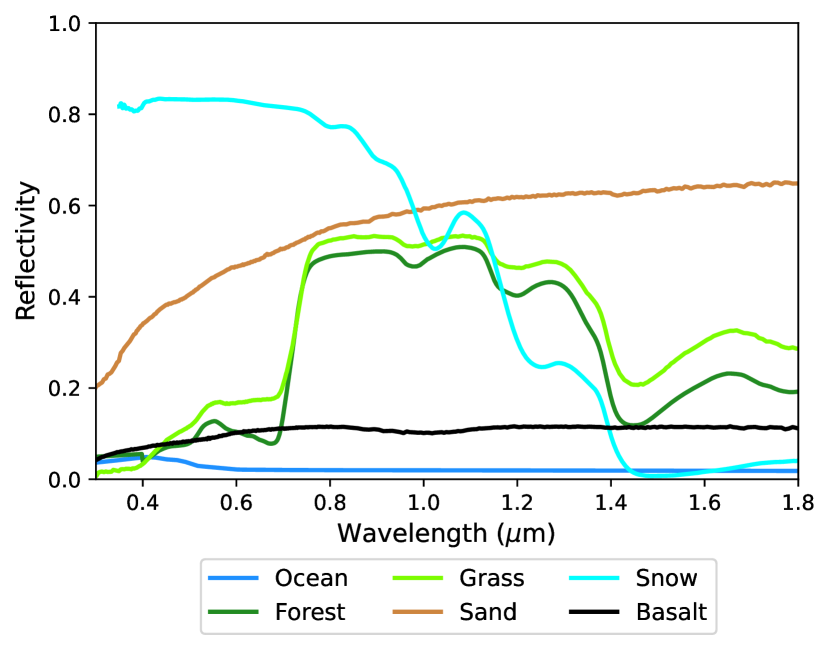
Figure 1: The six main surface albedos used in our Earth Through Time models, taken from the NASA JPL EcoStress Spectral Library and the USGS Spectral Library. Note the strong VRE in the grass and forest surfaces.

Our planet surfaces are modeled as ideal, depolarizing Lambertian surfaces with wavelength-dependent albedos. This is a common approximation in Earth modeling and retrievals (see, e.g., Tilstra et al., 2021, and references therein), even though for many surfaces of interest for habitability studies, like vegetation, it can lead to errors in the retrieved properties (e.g., Lorente et al., 2018). We acknowledge that to model surfaces more accurately, bidirectional reflection (or polarization) distribution functions (BRDF/BPDF), which take into account changes in the reflected flux (or polarization) as a function of illumination and viewing angles, are needed. For example, ocean surfaces can often be wavy and rough, displaying specular features, and are best modeled as Fresnel surfaces with whitecaps (see, e.g., Trees & Stam, 2019; Vaughan et al., 2023, and references therein). However, the disk-integrated signals of exoplanets may result in a smearing of the surface reflectance, so Lambertian surfaces are expected to provide sufficient approximations (see, e.g., Stam, 2008; Kopparla et al., 2018; Gordon et al., 2023). We therefore stick with Lambertian surfaces for the models presented in this study. Modeling BPDF surfaces for vegetation and Fresnel-reflecting surfaces for oceans is part of ongoing future work.

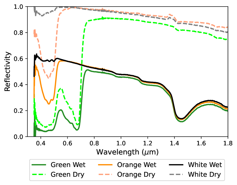
Figure 2: The surface albedos of the three biological species chosen from The Color Catalogue of Life in Ice (Coelho et al., 2022) for our Earth Through Time models. Solid lines correspond to the fresh samples directly after collection, and the dashed lines to the same samples after they have dried.

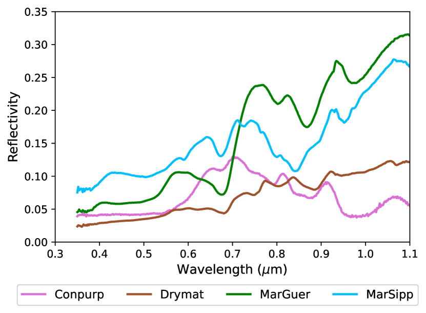
Figure 3: The four microbial surface albedos described by Sparks et al. (2021). These spectra were only observed over a wavelength range of $\lambda$ = 0.35 - 1.1 $\mu$m.

Here we modeled seven different categories of surfaces: ocean, forest (a combination of deciduous and conifer), grass, sand, melting snow, fresh basalt, and microbial surfaces. The reflection properties of the first six surfaces were taken from the NASA JPL EcoStress Spectral Library (Baldridge et al., 2009; Meerdink et al., 2019) as well as the USGS Spectral Library (Kokaly et al., 2017) and can be seen in Fig. 1.

For the microbial surfaces we used spectra from two different studies. For the majority of our models, including all models in Section 4, we utilized six reflection spectra from microorganisms found in the “Color Catalogue of Life in Ice” (Coelho et al., 2022). These microorganisms were organized into five groups based on the colors of their pigments: orange, yellow, green, pink, or white. Additionally, their reflection spectra were measured for both fresh (i.e., wet) samples directly after collection and then for the same samples $\sim$1 week after collection (i.e., dry). Here, we utilized one wet and one dry sample from the green, orange, and white pigment groups; specifically, the samples used correspond to Chlorophyta algae (green), Brevundimonas sp. (orange), and Bacillus sp. (white). The reflectance spectra for these six samples are shown in Fig. 2. Note the deep hydration feature around 1.4 $\mu$m in each of the wet samples that disappears in their corresponding dry samples. For more details regarding these samples, we refer the reader to Coelho et al. (2022).

The second group of microbial surfaces we used were collected from various sites by one of the authors of this paper (M. N. Parenteau) and maintained at NASA Ames Research Center. These spectra represent environmental anoxygenic and oxygenic photosynthetic microbial mats. We used these mat samples to represent microbial surfaces that arose during the Archean and Proterozoic eons (see Sections 3.4.4 and 3.4.5). In particular, for microbial mats on emerging continents during these time periods we used spectra of a dry Phormidium mat (hereafter, Drymat) and a planktonic purple sulfur pool (hereafter, Conpurp). For microbial mats in shallow seas and coastal areas during these time periods we used spectra of a hypersaline mat from Guerrero Negro (hereafter, MarGuer) and a cyanobacteria mat from the Great Sippewissett Salt Marsh (hereafter, MarSipp). The reflectance spectra for these four samples are shown in Fig. 3. For more information about these samples, we refer the reader to Sparks et al. (2021), who measured the reflection and circular polarization spectra for all of these cultures and mats. In Section 5.2 we compare model spectra using these surfaces against those of Coelho et al. (2022).

3.4 Our Chosen Epochs

To capture the evolution of Earth through geological time we used inputs from multiple studies. The vertical mixing ratios (VMRs) for the five most spectroscopically significant molecules included in all of our modeled atmospheres are shown in Fig. 4. The T-P profiles for our six epochs are displayed in Fig. 5. Finally, Table 1 highlights the key atmospheric and surface properties for each case. For the stellar source for our calculations, we used the wavelength-dependent solar evolution correction developed by Claire et al. (2012) to scale the solar constant to the proper age for each epoch. These ages are also included in Table 1.

Figure 4: The change in the vertical mixing ratios for O₂, H₂O, CO₂, CO, and CH₄ over the evolution of Earth.

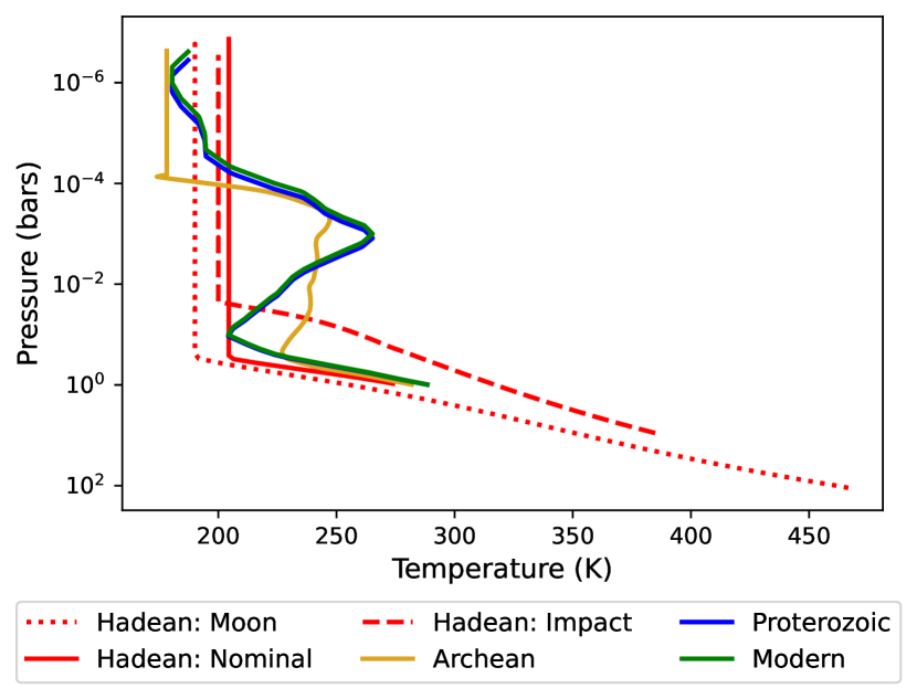
Figure 5: T-P profiles for our six Earth Through Time epochs. The surface pressure was much higher for the two impact-driven atmospheres of the Hadean eon (Hadean: Moon and Hadean: Impact), and the rise in atmospheric O₂ and the subsequent ozone layer led to a stronger temperature inversion in the later stages of Earth’s history (Proterozoic and Modern).

Table 1: Summary of key atmospheric and surface properties for our six Earth Through Time epochs. All surfaces are modeled as depolarizing Lambertian surfaces with wavelength-dependent albedos (see Figs. 1 - 3).

Epoch	Age (Ga)	Main Atmospheric Gases	Surface	$A_{G}$ ($\lambda$ = 0.5 $\mu$m, 0.9 $\mu$m)a
Hadean: Moon	4.45	CO2, N2, CO	95% ocean, 5% basalt	2.88, 0.26
Hadean: Nominal	4.2	N2, CO2, CO, H2	80% ocean, 20% basalt	0.43, 0.13
Hadean: Impact	4.0	H2, N2, CO2, CH4	70% ocean, 30% basalt	2.02, 0.02
Archean	2.7	N2, CO2, CH4	90% ocean, 8% Arch. landb,	0.47, 0.17
			2% early coastc
Proterozoic	2.5	N2, CO2, O2	85% ocean, 12% Proto. landd,	0.52, 0.25
			3% early coast
Modern	0	N2, O2, CO2, H2O	70% ocean, 8% forest, 8% grass,	0.59, 0.47
			5% snow, 4% sand, 4% basalt,
			1% bioe

3.4.1 Hadean Earth after Moon Forming Impact

Shortly after the formation of the Earth around 4.54 Ga, it is thought that a Mars-sized proto-planet named Theia collided with the proto-Earth, with the resulting ejecta forming the Moon (e.g., Hartmann & Davis, 1975; Canup & Asphaug, 2001). This moon-forming giant impact would have melted the entire proto-Earth mantle down to the core, resulting in a global magma ocean. All volatile elements (including, e.g., H₂O, CO₂, etc.) would have then partitioned between the magma and the atmosphere according to their solubility. Since water is much more soluble in magma than CO₂ (e.g., Blank & Brooker, 1994; Gardner et al., 1999), most of the water from proto-Earth would have been contained in the magma ocean, while most of the total reservoir of CO₂ (about 100 bar) would be in the atmosphere (e.g., Zahnle et al., 2010). The magma would solidify in $\sim$1-2 million years, followed by a rapid condensation of the ocean, leaving behind a warm $\sim$500 K planet with 100 bars of CO₂ and a shallow liquid ocean (e.g., Zahnle et al., 2007). Indeed, the oldest found zircon crystals are believed to be as old as $\sim$4.4 Ga (e.g., Wilde et al., 2001), suggesting that liquid water formed on proto-Earth rather early. Although continental crust was most likely absent, high levels of activity from mantle plumes probably created multiple exposed ocean islands (see, e.g., Korenaga, 2021, and references therein). The CO₂ in the atmosphere probably then reacted with the exposed seafloor during the planetary cooling process and subducted back into the planet, thereby removing the thick CO₂ atmosphere in 20-100 million years(e.g., Zahnle et al., 2010).

Our first Hadean Earth model (hereafter, Hadean: Moon) is a simulation of the Earth when the atmosphere was CO₂-dominated for 20-100 million years after the moon-forming giant impact. This atmosphere also contained large amounts of N₂ and H₂O as well as trace amounts of CO, H₂, CH₄, and O₂. The surface was dominated by a shallow ocean with about 5% of the globe also covered by basaltic exposed islands.

3.4.2 Nominal Hadean Earth

For the majority of the Hadean eon ($\sim$4.54 - 4.03 Ga), the early Earth potentially had an N₂-CO₂ dominated atmosphere with trace amounts of volcanic and photochemical H₂ and CO (e.g., Catling & Zahnle, 2020). Additionally, large amounts of continental crust could have developed as the Earth continued to cool from the moon-forming giant impact (e.g., Guo & Korenaga, 2020). The growth of the continents could have outpaced the condensation of the still-shallow ocean, and ocean islands from mantle plumes continued to provide more exposed land, such that approximately 20% or more of the Earth’s surface could have been covered by exposed continental crust (e.g., Korenaga, 2021).

Our second Hadean Earth model (hereafter, Hadean: Nominal) is a simulation of the Earth during the mid-Hadean when it had a 1 bar N₂-dominated atmosphere with 10% CO₂ and trace amounts of O₂ and H₂O. Our photochemical simulations also assumed that CO, H₂, SO₂, and H₂S were emitted to the atmosphere at rates calculated in Wogan & Catling (2020). As with the Hadean: Moon model, the surface of our Hadean: Nominal model was dominated by a shallow ocean but now with 20% of the Earth covered by exposed basaltic crust.

3.4.3 Hadean Earth after Asteroid Impact

Throughout the Hadean eon Earth was struck by asteroid impactors. The largest of these impactors possessed cores that would have delivered metallic iron that could potentially reduce the atmosphere and vaporize the ocean, even potentially melting the crust down a few tens of kilometers (e.g., Zahnle et al., 2010, 2020). This would have created a transient H₂-CH₄-N₂-CO₂ atmosphere that more closely resembles Neptune’s than modern Earth’s. Additionally, a large impact combined with a relatively dry early-Earth stratosphere could allow for the buildup of thick photochemical hazes. The transient, hazy atmosphere would have lasted for millions of years until the hydrogen escaped to space and the skies cleared (e.g., Zahnle et al., 2020; Wogan et al., 2023).

Our third Hadean Earth model (hereafter, Hadean: Impact) is a snapshot of the Hadean atmosphere towards the end of the eon, $\sim$15,000 years after a Ceres-sized ($\sim$900 km) asteroid impact. We modeled a $\sim$9 bars, H₂-dominated atmosphere with large amounts of CH₄, N₂, and CO₂ that was rich in hydrocarbon haze. Our photochemical simulations also assumed trace amounts of O₂, H₂O, CO, HCN, and NH₃. As with our two previous Hadean Earth models, the surface of our Hadean: Impact model was dominated by an ocean but now with 30% of the Earth covered by basaltic crust that was exposed due to the impact.

3.4.4 Archean Earth

The Archean eon began $\sim$4.03 Ga and lasted until the first hypothesized Snowball Earth during the Huronian glaciation event, when our atmosphere began transitioning from anoxic to oxic with the first substantial rise in O₂ ($\sim$2.5 Ga; e.g., Tang & Chen, 2013; Young, 2019). From the early to mid-Archean, the Earth was mostly a water world (e.g., Korenaga, 2021). Towards the end of the eon, increased mantle convection and tectonic activity is believed to have caused several cratons to rise above the ocean surface and combine into the first supercontinents (e.g., de Kock et al., 2009; Rogers, 1996; Bindeman et al., 2018; Williams et al., 1991). It is also assumed that the Archean was the first geologic eon with a prevalent microbial biosphere (e.g., Dodd et al., 2017; Djokic et al., 2017; Allwood et al., 2006), although the precise timing of the emergence of the first life on Earth is not known. The atmosphere during this eon is thought to have had very low levels of O₂, which could have supported the formation of an organic haze generated by CH₄ photolysis (e.g., Claire et al., 2014).

Our Archean Earth model is a simulation of the Earth after the evolution of oxygenic photosynthesis but prior to any substantial increase in O₂ in the atmosphere. We used the Archean Earth atmospheric model from Arney et al. (2016), which assumed a weakly reducing atmosphere dominated by N₂ and CO₂ with large amounts of CH₄ and CO. This atmosphere also included H₂O and H₂ as well as small amounts of atmospheric O₂ and NO. As in Arney et al. (2016), our Archean atmosphere was rich in hydrocarbon haze similar to modern-day Titan. The surface of our Archean model was dominated by a deep ocean and included a single supercontinent covering $\sim$10% of the globe (Bindeman et al., 2018). 2% of this land we modeled as coastal regions with 50% sand and 50% microorganisms, and the remaining 8% was a combination of basalt, sand, and microorganisms.

3.4.5 Proterozoic Earth

The Proterozoic eon was the longest in Earth’s history, lasting from the first rise in O₂ concentration in the planet’s atmosphere and oceans ($\sim$2.5 Ga) to just before the appearance of diverse complex life ($\sim$0.5388 Ga). Multiple geological and ecological changes occurred throughout this eon, including the transition from a reducing to an O₂-rich atmosphere through the Great Oxidation Event (GOE) (e.g., Holland, 2006; Lyons et al., 2014); a series of global glaciation events (e.g., Tang & Chen, 2013); the rise and breakup of multiple new supercontinents (e.g., Rogers & Santosh, 2002; Li et al., 2008; Nance & Murphy, 2019); and the rise of eukaryotic organisms and multicellular life (e.g., Schirrmeister et al., 2013).

Our Proterozoic Earth model is a simulation of the Earth at the beginning of the eon, before the start of the GOE but after the introduction of more O₂ in the atmosphere from cyanobacteria. We utilized the Proterozoic Earth atmospheric model from Arney et al. (2016), which assumed an N₂-dominated atmosphere still with large levels of CO₂ and atmospheric H₂O but with 0.1% the present atmospheric level of O₂, consistent with the findings in Planavsky et al. (2014). These photochemical simulations also predicted trace amounts of CH₄, H₂, CO, and O₃. The surface of our Proterozoic model was dominated by a deep ocean with 15% of the globe covered by land. 3% of this land was modeled as coastal regions with 50% sand and 50% microorganisms, and the remaining 12% was a combination of basalt, sand, microorganisms, and snow.

3.4.6 Phanerozoic (Modern) Earth

As Earth’s current geologic eon, the Phanerozoic eon began with the Cambrian explosion ($\sim$0.5388 Ga) (e.g., Marshall, 2006) that marked the rapid proliferation and diversification of complex life. Effects of this complex life, specifically those from vegetation, on the planet’s climate and resulting flux can be seen in observations of earthshine (e.g., Woolf et al., 2002; Pallé et al., 2009). Increased vegetation also led to the last major rise in atmospheric O₂ and the strengthening of the ozone layer (e.g., Kasting & Donahue, 1980; Segura et al., 2003). Tectonic forces collected the existing landmasses into the most recent supercontinent Pangaea (e.g., Dietz & Holden, 1970), which then separated into the current continents.

Our Modern Earth model is a simulation of the Earth as it appears today. The atmosphere is N₂-dominated with 21% O₂ and $\sim$0.0366% CO₂, followed by present-day trace amounts of CO, CH₄, O₃, N₂O, and NO. The surface of our Modern Earth is covered by 70% deep oceans, 5% snow, and 25% land that is dominated by vegetation (i.e., forest and grass).

4 Results & Comparisons

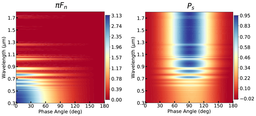
Figure 6: Reflected total normalized flux $\pi{F_{n}}$ (left panel) and signed degree of linear polarization P_s (right panel) as functions of the planetary phase angle $\alpha$ and wavelength $\lambda$ for our Hadean: Moon model. Note the differences in the colorbars for the two plots.

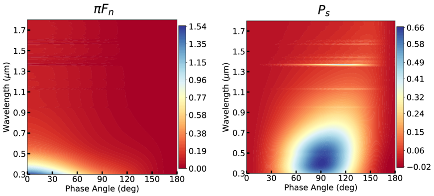
Figure 7: Same as Fig. 6, except for our Hadean: Nominal model.

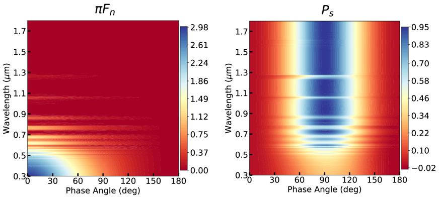
Figure 8: Same as Fig. 6, except for our Hadean: Impact model with a clear atmosphere.

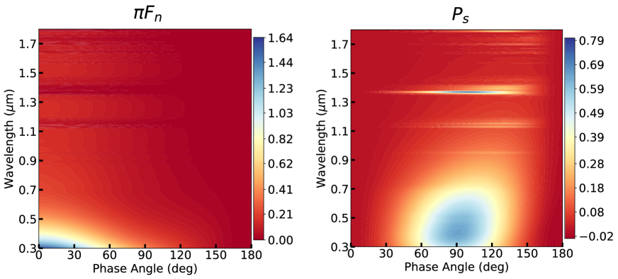
Figure 9: Same as Fig. 6, except for our Archean model with a clear atmosphere.

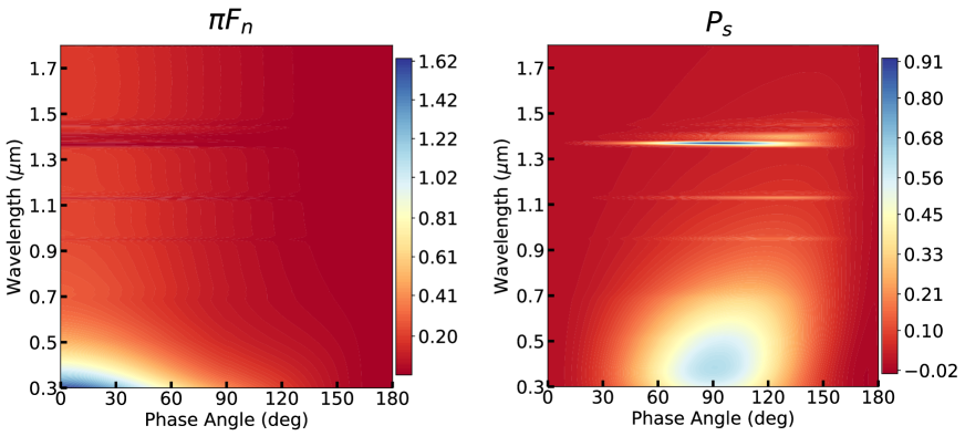
Figure 10: Same as Fig. 6, except for our Proterozoic model with a clear atmosphere.

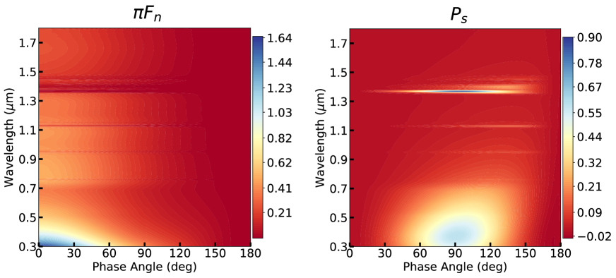
Figure 11: Same as Fig. 6, except for our Modern model with a clear atmosphere.

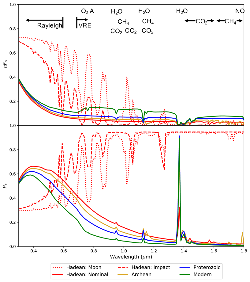
Figure 12: Cross-sections through the left (top panel) and right (bottom panel) panels of Figs. 6 - 11 at $\alpha=90\degree$ to show the spectral differences of each of our six Earth Through Time epochs. Note the distinguishing spectral features of different species across different epochs as well as a noticeable VRE in our Modern Earth model.

In this section, we present the total normalized flux and signed degree of linear polarization signatures of starlight reflected by our six Earth Through Time epochs. Our models have a constant $\Delta\lambda$ of 10 nm, corresponding to spectral resolving powers of R_VIS $\sim 50$ and R_NIR $\sim 150$. Unless otherwise stated, our models were generated using the DAP code.

4.1 Clear Atmospheres

Fig. 6 through Fig. 11 display the total normalized flux ($\pi{F_{n}}$) and signed degree of linear polarization (P_s) of the reflected flux as functions of both $\lambda$ and $\alpha$ for our six epochs. All of these models possess clear (i.e., cloud- and haze-free) atmospheres, with atmospheric species and surfaces described in detail in Section 3.4 and highlighted in Table 1.

P_s for all six models peak around $\alpha$ = 90$\degree$ due to Rayleigh scattering and the large contribution of the dark ocean on each surface (see Fig. 1 and Table 1), as expected (see, e.g., Hansen & Travis, 1974; Stam, 2008). Similarly, $\pi{F_{n}}$ peaks at $\alpha$ = 0$\degree$ (i.e., when the planet is fully illuminated) and decreases smoothly with phase until $\alpha$ = 180$\degree$ (i.e., when we see the planet’s night side). All models also show the planets are brighter (i.e., larger $\pi{F_{n}}$) at shorter $\lambda$, where the atmospheric optical thickness is the largest, and gradually get darker with increasing $\lambda$. The hotter atmospheres and higher surface pressures (see Fig. 5) of the Hadean: Moon and Hadean: Impact scenarios, combined with higher concentrations of CO₂ and CH₄, respectively, in their atmospheres (see Fig. 4), increased the NIR absorption for these models. This darkened the planets and led to lower $\pi{F_{n}}$ compared to our other scenarios. The increased absorption diminished the multiply scattered background light, however, resulting in higher P_s for these models.

As future missions aimed at characterizing habitable worlds will be focusing on direct imaging and therefore will be optimized for viewing the planets near quadrature (i.e., $\alpha$ = 90$\degree$), Fig. 12 displays $\pi{F_{n}}$($\lambda$) and P_s($\lambda$) for all six models at $\alpha$ = 90$\degree$. The increase in global snow coverage and vegetation in the Modern model compared to the Archean or Proterozoic models leads to higher surface reflectivity, thereby increasing the $\pi{F_{n}}$ and lowering the P_s of the planet. Additionally, the VRE around 0.7 $\mu$m, due to absorption by chlorophyll in the vegetated surfaces, is apparent in both the $\pi{F_{n}}$ and P_s of the Modern spectra. The atmospheric evolution and resulting change in VMRs of key atmospheric species (see Fig. 4) leads to different features dominating the spectra over time, thereby differentiating the model Earths across the epochs. Most noticeable are the strongly polarized NIR H₂O bands near 0.93, 1.12, and 1.35 - 1.4 $\mu$m whose depths change depending on their respective mixing ratios in their models. We can also see the strong O₂ A-band at 0.76 $\mu$m in the Modern model; the 1.15, 1.64, and 1.72 $\mu$m CH₄ bands and 1.78 $\mu$m NO band in the Archean model; and the 1.44 $\mu$m CO₂ band in the Proterozoic and Modern models.

4.2 Effects of Clouds and Hazes

Aerosols in an atmosphere play a significant role in determining the overall polarization state of the planet. Fig. 13 shows our Proterozoic epoch model at quadrature for three different cases: a clear atmosphere (green solid lines), an atmosphere with a layer of Cirrus clouds (dotted blue lines), and an atmosphere with a layer of Stratocumulus clouds (dashed red lines); see Section 3.2 for the properties of these clouds. As expected, the addition of water clouds in the atmosphere reduces or even flattens some absorption and surface features, and the increased albedo of the cloud droplets and multiple scattering within the clouds lead to higher $\pi{F_{n}}$ and lower P_s. While the Stratocumulus clouds are more optically thick than the Cirrus clouds, the higher altitude of the latter block more light from reaching lower in the atmosphere than the former, thus further suppressing the 1.4 $\mu$m H₂O absorption. We can see that P_s does a better job than $\pi{F_{n}}$ at distinguishing the three models. While the normalized flux spectra between the clear and Cirrus cases overlap across multiple wavelengths, with the maximum absolute difference in $\pi{F_{n}}$ being $\sim$0.035 in the 1.4 $\mu$m H₂O band and $\sim$0.025 in the continuum, the polarization spectra show clear separation between the models, with the maximum absolute difference in P_s being $\sim$0.9 in the 1.4 $\mu$m H₂O band and $\sim$0.125 in the continuum.

Fig. 14 displays phase curves of $\pi{F_{n}}$ and P_s in different observational bands for our Proterozoic model with Stratocumulus clouds. Phase curves from our clear atmosphere Proterozoic model are also included at r^′ band for comparison (dashed black lines). As expected, the clear atmosphere model shows the smooth decrease of $\pi{F_{n}}$ towards larger $\alpha$ and the peak P_s around $\alpha$ $\approx$ 90 - 100$\degree$. P_s is more sensitive to the introduction of clouds than $\pi{F_{n}}$, and although the $\pi{F_{n}}$($\alpha$) for all $\lambda$s overlap and are therefore indistinguishable, the P_s($\alpha$) show the wavelength dependence of the rainbow feature for the liquid water clouds, with the rainbow peak shifting to smaller $\alpha$ with increasing $\lambda$ (see e.g., Bailey, 2007; Karalidi et al., 2012). Additionally, the rainbow feature becomes stronger with increasing $\lambda$, becoming a global maximum in P_s($\alpha$), and its strength can change depending on the cloud altitude and optical thickness (for more details, see e.g., Gordon et al., 2023).

Fig. 15 shows the influence of hydrocarbon haze in the atmosphere of our Hadean: Impact scenario on the resulting planetary $\pi{F_{n}}$($\lambda$) and P_s($\lambda$) at quadrature. Due to their opaque nature the hazes block the light from reaching lower in the atmosphere, thereby flattening the spectra and reducing NIR absorption features but increasing the reflectivity of the planet at these longer wavelengths. As in Arney et al. (2016), the hazes also result in reddening of the unpolarized light color of the planet. The increased UV absorption combined with increased scattering within the aerosol particles decreases the $|$P_s$|$ of the light in the visible but increases it in the UV. The change in sign of P_s to negative in the UV (i.e., the light is now polarized parallel to the scattering plane) is due to first order scattered light from the aerosol particles (see, e.g., Karalidi et al., 2011, 2013).

Fig. 16 shows $\pi{F_{n}}$($\alpha$) and P_s($\alpha$) at different observational bands for a homogeneous ocean planet (i.e., the entire surface is now modeled as a depolarizing Lambertian ocean; see Section 3.3 and Fig. 1) with an Archean atmosphere containing hydrocarbon haze. For comparison, phase curves from a homogeneous ocean planet with a clear Archean atmosphere are also included at i^′ band (dashed black lines). Similar to the water clouds of Fig. 14, the increased multiple scattering within the hazes brightens the planet compared to the clear atmosphere case, leading to larger $\pi{F_{n}}$. However, unlike the cloudy models, which show a nearly wavelength-independent increase in $\pi{F_{n}}$, the hazes absorb more light at shorter $\lambda$ and scatter more light at longer $\lambda$, thereby displaying a wavelength-dependence for $\pi{F_{n}}$. Additionally, both the $\pi{F_{n}}$ and P_s curves show wavelength-dependent features for the hazes that smooth out with increasing $\lambda$, with P_s being more sensitive to the addition of hazes than $\pi{F_{n}}$. While the water clouds of Fig. 14 show a single rainbow feature at $\alpha$ $\approx$ 40$\degree$ polarized perpendicular to the scattering plane, the hazy models show multiple features that are instead polarized parallel to the scattering plane and whose locations shift in $\alpha$ with changing $\lambda$. We acknowledge, however, that these features, especially the multiple undulations at shorter $\lambda$, could be non-physical artifacts from using spherical Mie-scattering particles for these model hazes (see Section 3.2) and therefore might not be observed in an exoplanet. We discuss the effects of using Mie vs. fractal scattering haze particles in more detail in Section 5.1.

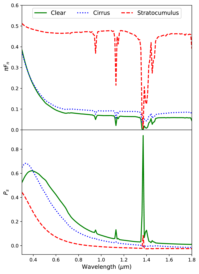
Figure 13: $\pi{F_{n}}$($\lambda$) (top) and P_s($\lambda$) (bottom) from our Proterozoic model for atmospheres that are: clear (solid green lines), with Cirrus clouds (dotted blue lines), or with Stratocumulus clouds (dashed red lines). All models are shown at quadrature. The addition of clouds increases the reflectivity of the planet but flattens the spectra, especially at shorter $\lambda$. The three models are more easily distinguishable in P_s.

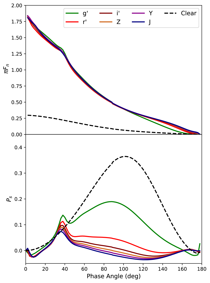
Figure 14: $\pi{F_{n}}$($\alpha$) (top) and P_s($\alpha$) (bottom) from our Proterozoic model with Stratocumulus clouds, shown at the center $\lambda$ of various bandpasses. For comparison, curves from our Proterozoic model with clear atmospheres are also shown for r^′ band (dashed black lines). Diagnostic features of the liquid water clouds (primary rainbow at $\alpha\approx$ 40$\degree$) can be seen slightly in $\pi{F_{n}}$($\alpha$) and more clearly in P_s($\alpha$).

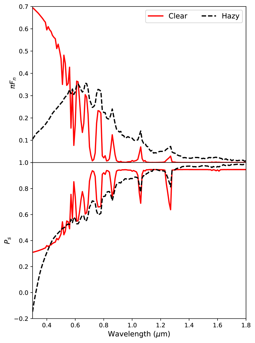
Figure 15: $\pi{F_{n}}$($\lambda$) (top) and P_s($\lambda$) (bottom) at $\alpha$ = 90$\degree$ for our Hadean: Impact model with either a clear (solid red lines) or hazy (dashed black lines) atmosphere. Hazes flatten the spectra and flip the polarization of the short-wavelength light.

Figure 16: $\pi{F_{n}}$($\alpha$) (top) and P_s($\alpha$) (bottom) of a homogeneous planet with an ocean surface and Achean atmosphere containing hydrocarbon hazes, shown at the center $\lambda$ for various bandpasses. For comparison, curves of a homogeneous ocean planet with a clear Archean atmosphere are also shown for the i^′ band (dashed black lines). Features of the hazes are apparent in both plots but are more distinguishing in the P_s($\alpha$).

5 Impact of Fractals and Different Biomats

Our models of the Earth Through Time have so far assumed idealistic cases for the modeled aerosol particles and surfaces. These simplifications are typical for theoretical studies focused on modeling exoplanets (e.g., Luna & Morley, 2021), and can greatly decrease computational runtime and storage requirements, but can also have noticeable effects on the models (e.g., Feng et al., 2018; Gordon et al., 2023). In this section we explore the influences of more physically-realistic cloud and haze particles as well as different microbial surfaces on the resulting $\pi{F_{n}}$ and P_s of our Earth Through Time models.

5.1 Mie vs. Fractal Scattering in Clouds & Hazes

In Section 4 we used Mie theory (i.e., spherical particles) to calculate the scattering properties of our cloud and haze particles. However, in reality H₂O ice clouds are composed of crystals of varying shapes and sizes depending on the temperature and humidity of their environment (e.g., Magono & Lee, 1966; Heymsfield & Platt, 1984). Additionally, hydrocarbon haze is composed of chains of smaller monomer molecules that link and clump together to form aggregates (e.g., Bar-Nun et al., 1988; Cabane et al., 1993). The optical properties of both of these particles can be better approximated using fractal scattering models (e.g., Mishchenko et al., 2000). Fractal particles tend to produce less extinction and be more forward-scattering in the VNIR compared to equal-mass spherical particles (see, e.g., Arney et al., 2016, 2017; Wolf & Toon, 2010).

Fig. 17 compares $\pi{F_{n}}$($\alpha$) and P_s($\alpha$) between models of Modern atmospheres with a depolarizing Lambertian ocean surface (see Section 3.3 and Fig. 1) and Cirrus clouds, whose particles were generated either with Mie scattering (solid lines) or fractal scattering (dashed lines). The cloud particles for the latter models were generated using scattering matrices of imperfect hexagonal ice polycrystals whose sizes range from $\sim$6 $\mu$m to $\sim$2 mm, at wavelengths of 0.55 (green lines), 0.66 (orange lines), and 0.865 $\mu$m (red lines) (see Hess et al., 1998; Karalidi et al., 2012, and references therein for more details).

Due to increased scattering off of and within the fractal crystals, the fractal ice clouds reflect more light than the Mie-scattering ice clouds, especially near $\alpha$ $\approx$ 90$\degree$ (see Karalidi et al., 2012, their Fig. 3 and Fig. 4, for the single scattering phase functions of the ice particles). At larger $\alpha$, most of the reflected light has been scattered by the gas molecules in the atmospheric layers above the clouds, therefore decreasing the influence of the clouds. This leads to higher levels of background unpolarized light that lowers P_s for both types of clouds. However, the larger size of the fractal ice crystals compared to the spherical ice particles leads to more absorption of the light that is not scattered at these larger $\alpha$, resulting in lower $\pi{F_{n}}$ and higher P_s at $\alpha>$ 120$\degree$.

As expected, both types of cloudy models show Rayleigh peaks, caused by scattering by the gas molecules above the clouds, in their P_s($\alpha$) that decrease with increasing $\lambda$. Note that the Mie ice clouds, like the liquid water clouds in Fig. 14, show a primary rainbow feature around $\alpha$ = 40$\degree$. The P_s of the ice cloud rainbow is larger than that of the liquid water clouds due to the larger particle sizes (e.g., Gordon et al., 2023). The fractal ice clouds, however, do not show this feature, in agreement with Earth observations (see, e.g., Karalidi et al., 2012, and references therein).

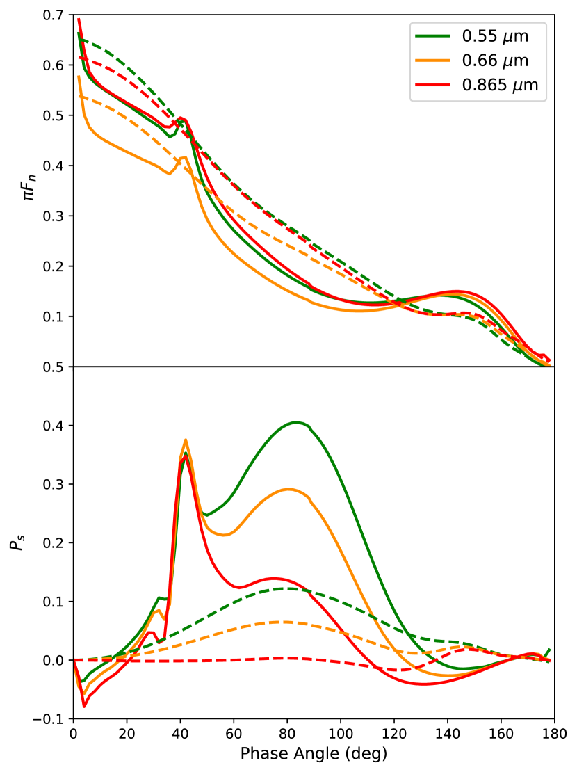
Figure 17: $\pi{F_{n}}$($\alpha$) (top) and P_s($\alpha$) (bottom) for a homogeneous planet with an ocean surface and Modern Earth atmosphere containing Cirrus clouds, at $\lambda$ = 0.55 $\mu$m (green lines), 0.66 $\mu$m (orange lines), and 0.865 $\mu$m (red lines). The clouds are made of either spherical (solid lines) or fractal (dashed lines) particles.

In Fig. 18 we show $\pi{F_{n}}$($\alpha$) and P_s($\alpha$) of an ocean planet with a Hadean: Impact atmosphere containing either Mie (solid lines) or fractal scattering (dashed lines) hazes. For the fractal hazes, we used the haze particles of Karalidi et al. (2013), which are modeled as randomly oriented aggregates of 94 equally sized spheres that coagulate through a cluster-cluster aggregation method into a particle with a volume-equivalent-sphere radius of 0.16 $\mu$m (Karalidi et al., 2013). The optical properties of the particles were calculated at $\lambda$ = 0.55, 0.75, and 0.95 $\mu$m using the T-matrix theory combined with the superposition theorem (Mackowski & Mishchenko, 2011), with a wavelength-independent complex refractive index of 1.5 $\pm$ 0.001i (Karalidi et al., 2013).

Because the fractal particles are made of monomers, the light is scattered more within each particle in comparison to the spherical particles, therefore increasing the $\pi{F_{n}}$ but decreasing the P_s from the haze compared to those of the spherical particles (e.g., Karalidi et al., 2013). Both $\pi{F_{n}}$($\alpha$) and P_s($\alpha$) for both types of hazes are relatively featureless due to the small sizes of the particles, with Rayleigh scattering dominating the curves. While the disk-integrated P_s of the Mie hazes peaks at $\alpha\approx$ 90$\degree$ for all three $\lambda$, the fractal hazes show a wavelength-dependent shift in the peak towards larger $\alpha$.

Figure 18: $\pi{F_{n}}$($\alpha$) (top) and P_s($\alpha$) (bottom) of a homogeneous planet with an ocean surface and Hadean: Impact atmosphere containing hydrocarbon hazes, at $\lambda$ = 0.55 $\mu$m (green lines), 0.75 $\mu$m (red lines), and 0.95 $\mu$m (black lines). The hazes are made of either spherical (solid lines) or fractal (dashed lines) particles.

5.2 Biomat Surface Reflectances

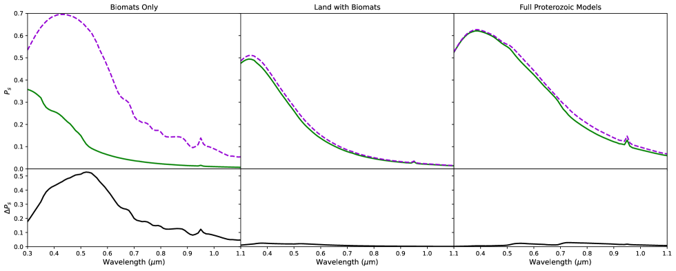
Figure 19: Comparisons at quadrature of P_s($\lambda$) between Proterozoic models with clear atmospheres and biological surfaces from Coelho et al. (2022) (solid green lines) or Sparks et al. (2021) (dashed purple lines). As we zoom out (from left to right) from a pixel to a Proto. land to a full planet view, the reduction in surface microbial coverage (100%, 5%, and 2.1%, respectively) results in smaller differences on the resulting disk-integrated P_s($\lambda$) for our weighted-averaged models. Absolute differences between the two spectra in each panel are shown in the bottom row.

Microbial surfaces can provide additional signatures to search for life on exoplanets (e.g., Schwieterman et al., 2015). Here, we used two databases, those of Sparks et al. (2021) and of Coelho et al. (2022), to test the detectability of microbes in our planetary signals. In Fig. 19 we compare P_s($\lambda$) at $\alpha$ = 90$\degree$ for our Proterozoic models with cloud-free atmospheres and biological surfaces from either Coelho et al. (2022) (like those used in Section 4; solid green lines) or Sparks et al. (2021) (dashed purple lines). Due to the limited wavelength range over which the biological surfaces of the latter studies were measured, the models in this section only cover wavelengths from 0.3 to 1.1 $\mu$m.

At the individual pixel scale (top left panel), where the entire surface is covered by either orange and white pigments or continental microbial mats, the Sparks et al. (2021) model reaches P_s $\approx$ 0.7, while the Coelho et al. (2022) model reaches P_s $\approx$ 0.35. The maximum absolute difference, $\Delta$P_s($\lambda$), between the spectra reaches $\sim$0.53 at $\lambda$ = 0.53 $\mu$m (bottom left panel). These differences are due to the higher albedos of the Coelho et al. (2022) microbial surfaces (see Fig. 2). At the Proto. land scale (top middle panel; see Table 1), the effects from the microbial surfaces on the resulting spectra decrease dramatically due to the microbes now covering only 5% of the model surface, with a maximum $\Delta$P_s($\lambda$) of $\sim$0.025 at $\lambda$ = 0.38 $\mu$m (bottom middle panel). At the full planet scale (top right panel), the maximum $\Delta$P_s($\lambda$) only reaches $\sim$0.028 at $\lambda$ = 0.73 $\mu$m (bottom right panel) due to the small percentage of microbes on the surface ($\sim$2.1%) compared to, e.g., the planetary ocean (85%). The changes in the wavelengths and values of the maximum $\Delta$P_s across the three panels is due to the different combinations of surfaces in the models, with the introduction of the green pigments and marine intertidal microbial mats in the full planet models shifting the maximum $\Delta$P_s to longer $\lambda$. Our results show that while the different microbial surfaces strongly influence P_s of local regions on our model planets, integrated across larger regions or the entire planetary disk, the microbial surfaces have a smaller influence on the resulting signal.

6 Observing Constraints for the Next Generation Telescopes

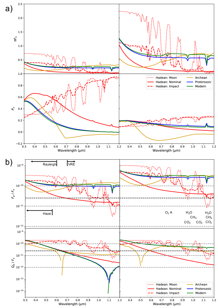
Figure 20: (a) $\pi{F_{n}}$($\lambda$) (top row) and P_s($\lambda$) (bottom row) for the full models of our six Earth Through Time epochs, with their atmospheres containing patchy clouds and hazes where applicable. The spectra are plotted at either quadrature (left column) or $\alpha$ = 40$\degree$ (right column). (b) Unpolarized (top row) and polarized (bottom row) contrast ratios for the six models of panel (a) scaled to their corresponding solar spectra through time. These contrast ratios assume the planets are in circular edge-on orbits. Also marked are contrast ratio limits of 1 $\times$ 10^-10, 1 $\times$ 10^-11, and 1 $\times$10 ^-12 (dashed grey lines), as well as the preliminary HWO lower limit of 2.5 $\times$ 10^-11 (dashed black lines). The breaks in some of the $Q{{}_{p}}/F{{}_{s}}$ curves are due to the polarized light changing directions (see Eq. 7). Note the distinguishing spectral features of different species across different epochs as well as a detectable VRE in our Modern Earth model.

The National Academy of Sciences Astronomy & Astrophysics 2020 Decadal Survey (hereafter Astro2020) recommended a new “Great Observatories” program telescope with the priority capability of “direct imaging to probe polarized ocean glint on terrestrial planets” (National Academies of Sciences, Engineering, and Medicine et al., 2021). The NASA Habitable Worlds Observatory (hereafter HWO), recently announced in response to these recommendations from Astro2020, is expected to draw heavily from the designs of proposed missions including LUVOIR (e.g., The LUVOIR Team et al., 2019) and HabEx (e.g., Gaudi et al., 2020). However, the full performance and capabilities of HWO are yet to be determined, and plans for different instruments are still in development.

With this in mind, we discuss here the detectability of our six different Earth Through Time models around an evolving solar-type star (Claire et al., 2012). To calculate the unpolarized planet-to-star contrast ratios, $F{{}_{p}}/F{{}_{s}}$, we computed the total reflected flux, $F_{p}$($\lambda$, $\alpha$), from the exoplanet arriving at the observer. We then calculated the total stellar flux seen at the observer, $F_{s}$($\lambda$):

$$F_{s}=\frac{L}{4\pi d^{2}}$$ (11)

where L is the stellar luminosity calculated from the incident flux $F_{0}$ at our model planet at an orbital distance $a$ away from the star, such that $L=F_{0}*4\pi{a^{2}}$. By combining Eqs. 8 and 11, we find that the unpolarized contrast ratios are given by:

$$\frac{F_{p}}{F_{s}}=\frac{1}{4}\textbf{S}(\lambda,\alpha)\left({\frac{r}{a}}\right)^{2}.$$ (12)

To obtain the polarized contrast ratios, $Q{{}_{p}}/F{{}_{s}}$, we multiply the $F{{}_{p}}/F{{}_{s}}$ for each model by the absolute value of its corresponding P_s (see Eq. 7). Additionally, since the majority of sun-like stars are unpolarized (e.g., Kemp et al., 1987; Cotton et al., 2017), observing our star-planet system in linearly polarized light (i.e., using a linear polarizer) allows us to reduce the stellar contribution by half for these polarized contrast ratios, since only half of the randomly-oriented stellar photons can pass through the linear polarizer (e.g., Collett, 2005). For our calculations here, we used a planetary radius $r$ = $R_{\earth}$ and an orbital distance $a$ = 1 AU. We acknowledge that these contrast ratios can also depend on the phase angle and inclination of the planet, but for simplicity, we assume circular edge-on orbits (i.e., $i$ = 90$\degree$).

Panel (a) of Fig. 20 shows $\pi{F_{n}}$($\lambda$) (top row) and P_s($\lambda$) (bottom row) for the full models of our six Earth Through Time epochs, while panel (b) shows the resulting unpolarized (top row) and polarized (bottom row) contrast curves for these epochs. We display here two key phase angles: $\alpha$ = 90$\degree$, to capture the planets at their widest inner working angle (IWA) (left columns), and $\alpha$ = 40$\degree$, to capture the planets at the peak of the water cloud rainbow feature (right columns). For computational efficiency, our models and contrast ratios here only cover $\lambda$ = 0.3 - 1.2 $\mu$m. This wavelength range still includes key atmospheric absorption features and surface biosignatures, and covers the recommended continuous wavelength ranges for both the HabEx and LUVOIR science cases (see, e.g., Mennesson et al., 2016; Mamajek & Stapelfeldt, 2024, and references therein). For the models that can possess hazes (Hadean: Impact and Archean), we assumed an equal distribution of 50% hazy and 50% clear atmospheres. For the models that can have water clouds (Proterozoic and Modern), we assumed that $\sim$67% of the planet was covered by clouds (e.g., King et al., 2013), which we divided up as 34% Cirrus clouds and 33% Stratocumulus clouds. The Hadean: Moon and Hadean: Nominal models have clear atmospheres here, although in reality we would expect some cloud cover during these eras. Due to the limited wavelengths over which the fractal aerosol particles were calculated in Section 5.1, our models here used the Mie-scattering aerosols of Section 3.2. Panel (b) of Fig. 20 also includes dashed grey lines denoting contrast ratio limits ranging from 1 $\times$ 10^-10 to 1 $\times$ 10^-12. Preliminary estimates of nearby target stars chosen for optimal HWO observations (Mamajek & Stapelfeldt, 2024) suggest a lower contrast ratio limit for the telescope of 2.5 $\times$ 10^-11 (denoted by the black dashed lines in the panel (b) plots).

In unpolarized light, we are able to resolve the VRE at $\sim$0.7 $\mu$m, O₂ A-band at 0.76 $\mu$m, and NIR H₂O absorption at 0.93 $\mu$m at both $\alpha$ in $F{{}_{p}}/F{{}_{s}}$ for the Modern Earth scenario above a contrast of 1 $\times$ 10^-10, the raw limit set by preliminary studies for LUVOIR and HabEx (e.g., The LUVOIR Team et al., 2019; Gaudi et al., 2020). At $\alpha$ = 90$\degree$, characterizing any additional absorption bands in the NIR requires a contrast ratio below this limit. Additionally, all three of the habitable planet scenarios (Archean, Proterozoic, and Modern) have $F{{}_{p}}/F{{}_{s}}$ above the HWO contrast limit at $\alpha$ = 90$\degree$. The hotter, highly-pressurized, and thus more absorbing Hadean: Moon and Hadean: Impact scenarios lead to lower contrasts in the NIR (down to $\sim$4.0 $\times$ 10^-12 and $\sim$1 $\times$ 10^-11, respectively) than the other four epochs, with the deep NIR CO₂ absorption bands in the Hadean: Moon model requiring contrasts lower than 1 $\times$ 10^-11. However, the stronger Rayleigh scattering in these models due to CO₂ (for the Hadean: Moon) and H₂ (for the Hadean: Impact) dominating their atmospheres leads to higher contrasts in the UV and VIS (up to $\sim$3.2 $\times$ 10^-10 and $\sim$1.9 $\times$ 10^-10, respectively). As discussed in Section 4.1, all models are brighter towards smaller $\alpha$ due to a larger portion of the visible disk being illuminated. This is detectable in the resulting $F{{}_{p}}/F{{}_{s}}$ of all six models at $\alpha$ = 40$\degree$. At this phase, all three habitable planet scenarios are detectable above the LUVOIR and HabEx raw limit of 1 $\times$ 10^-10 across the full spectrum, and all three Hadean scenarios are detectable above the HWO lower contrast limit, with the exception of the deepest NIR absorption bands. We acknowledge, however, that at smaller $\alpha$, the planet is closer to its host star and thus can be more difficult to observe, requiring tighter IWAs for the telescope to resolve it.

Since only a fraction of the light for each model planet becomes linearly polarized, the resulting $Q{{}_{p}}/F{{}_{s}}$ for all six epochs are lower than their corresponding unpolarized contrasts for both $\alpha$. As discussed in Section 4.1, the Hadean: Moon and Hadean: Impact scenarios have more absorption in the NIR than the other models, thus leading to less reflected flux at longer $\lambda$. However, any reflected light that does remain is singly scattered in the upper atmosphere and becomes highly polarized, leading to more reflected flux from the planet being detected and thus increasing $Q{{}_{p}}/F{{}_{s}}$ for these two scenarios. The breaks in $Q{{}_{p}}/F{{}_{s}}$ at $\lambda$ $\approx$ 1.1 $\mu$m for the Proterozoic and Modern scenarios at quadrature, as well as those at $\approx$ 0.65 $\mu$m (for $\alpha$ = 90$\degree$) and $\approx$ 0.5 $\mu$m (for $\alpha$ = 40$\degree$) for the Archean scenario, are not due to absorptions but rather to a change in the direction of the polarization (see Eq. 7), with the light switching from being polarized perpendicular (for shorter $\lambda$s) to parallel (for larger $\lambda$s) to the scattering plane. This is due to the introduction of the aerosols in these models, which changes the polarization state of the planets. Although the Hadean: Impact scenario also includes patchy hydrocarbon hazes here, the smaller $\tau$ and differing vertical distribution of particle radii modes (see Section 3.2) for the hazes in this model compared to those in the Archean scenario do not cause a change in the direction of the polarization. While the polarized contrasts for the Proterozoic and Modern models drop below 1 $\times$ 10^-12 at $\alpha$ = 90$\degree$ due to scattering by the liquid water clouds (see Section 4.2), these clouds create a peak in P_s at $\alpha$ $\approx$ 40$\degree$. At this phase, the $Q{{}_{p}}/F{{}_{s}}$ of these models are now detectable above the HWO contrast limit across the full spectrum.

Our calculated contrast ratios provide important preliminary predictions for the unpolarized and polarized planet-to-star flux ratios required to characterize Earth-like exoplanets across all evolutionary stages. Our results suggest that an Earth-like planet at any point in its history, from a young and hot Hadean-like planet to a current Modern-like planet, could be characterized around a Sun-like star in unpolarized (polarized) light if the contrast ratio capability of future instruments could be pushed to a lower limit of 1 $\times$ 10^-12 (1 $\times$ 10^-13).

7 Discussion And Conclusions

Earth has gone through many geological and ecological changes throughout its history, with evidence of life existing on the surface as early as the Archean eon. Comparing observations of Earth-like exoplanets only to the modern Earth therefore limits our characterizations of these worlds and our ability to assess their habitability. Previous studies that focused on the changes in Earth’s spectra through its evolution provided useful and important analyses but missed out on the full informational content available in the reflected light. In this work we presented the first numerical simulations of the spectropolarimetric signals of the Earth throughout its history, including, to our knowledge, the first unpolarized and polarized models of the spectra of the planet during the Hadean eon. Our models cover the full VNIR wavelength range ($\lambda$ = 0.3 - 1.8 $\mu$m, $\Delta$$\lambda$ = 10 nm) and the full phase angle space ($\alpha$ = 0$\degree$ - 180$\degree$, in 2$\degree$ steps). With the planned development of near-future polarimeters for both ground and space-based observatories, including the upcoming ELTs and HWO, as well as increased interest in polarization among the astrophysical community, we expect that these models can provide valuable feedback to the community. All of our Earth Through Time models are publicly available online through Zenodo: 10.5281/zenodo.13882511 (catalog doi:10.5281/zenodo.13882511).

For the clear (i.e., cloud- and haze-free) atmosphere planets modeled in Section 4, differences in the surface reflectivities and atmospheric VMRs across the different epochs allow us to distinguish between the habitable and non-habitable scenarios (see Fig. 12). The hotter atmospheres and higher surface pressures of the two short-lived, non-habitable Hadean scenarios cause increased absorption in the NIR, leading to lower $\pi{F_{n}}$ but higher P_s compared to the habitable scenarios. Additionally, while the Hadean: Nominal model produces similar $\pi{F_{n}}$ and P_s to the habitable scenarios, the lower levels of H₂O and higher levels of CO in its atmosphere compared to the other scenarios leads to distinguishing spectral features. The higher amounts of CH₄ in the Archean atmosphere and O₂ in the Modern atmosphere lead to detectable NIR absorption bands in the former and an O₂ A-band in the latter, thereby allowing for further differences between the habitable scenarios themselves.

The addition of clouds and hazes to our models flattens the resulting total flux and polarization spectra and reduces absorption and surface features, especially in P_s (see bottom panels of Fig. 13 and Fig. 15). The hydrocarbon hazes produce additional wide absorption features in the UV and VIS that darken the planets (i.e., lower $\pi{F_{n}}$, see top panel of Fig. 15) and invert the direction of the polarization (see bottom panel of Fig. 15). Additionally, while the spectra provide information on some absorption features for the cloudy and hazy models, phase curves provide important defining characteristics of the aerosols themselves, including the distinctive $\alpha$ $\approx$ 40$\degree$ rainbow feature of the liquid water cloud droplets (see Fig. 14). These aerosol features are more prominent in P_s than $\pi{F_{n}}$ for our models. Our results therefore highlight the importance of using both flux and polarization measurements across both wavelength and phase space to fully characterize the planets.

We acknowledge that our simplifications of a single cloud (haze) layer per pixel and the adoption of a single cloud (haze) size distribution across the planetary disk can affect the overall shapes of our model spectra and phase curves (e.g., Karalidi et al., 2012; Gordon et al., 2023). In reality, cloud particle sizes vary significantly across Earth, as do hazes across planets such as Jupiter and Titan, and these planets show overlap of clouds (hazes) with different properties (see, e.g., Han et al., 1994; Hess et al., 1998; Atreya et al., 2005; West et al., 2015, and references therein). Karalidi et al. (2012) modeled the Earth with overlapping layers of liquid water clouds of different size distributions, as well as liquid water clouds covered by ice clouds, and showed, for example, that the ice cloud coverage did not mask the liquid water rainbow feature at $\alpha$ $\approx$ 40$\degree$. For more information on the effects of overlapping clouds on the resulting $\pi{F_{n}}$ and P_s of terrestrial planets, we refer the reader to this study and the references within. In a future paper we plan to include models of terrestrial planets with changing amounts of clouds and hazes overlapping in the same atmospheres.

While assuming idealistic cases for atmospheric and surface models is common practice in simulating planetary signals (e.g., McLean et al., 2017; Tilstra et al., 2021), too many simplifications affect the models (e.g., Feng et al., 2018; Luna & Morley, 2021; Gordon et al., 2023). Here we showed that incorporating fractal scattering cloud and haze particles (Section 5.1) as well as different microbial surfaces (Section 5.2) create noticeable differences in our models. We acknowledge that changing levels of other surfaces would create similar variations in the polarized signals. The fractal clouds and hazes removed extraneous non-physical features in the resulting signals that were created by the Mie-scattering aerosols. Incorporating physically consistent model parameters will therefore be crucial for characterizing future observations and retrieving the true atmospheric and surface properties of potentially habitable exoplanets. However, we acknowledge that increasing the complexity of fitted models will increase the computing power and time needed to run them, so understanding which simplifications can be made to models in different scenarios without loss of necessary information will be vital.

To determine when we could detect noticeable differences in the disk-integrated P_s between spectra with the different microbial databases, we ran a preliminary parameter scan of models with microbial surface coverages ranging from 5% to 95% (in steps of 5%). We acknowledge that different combinations of surfaces can alter the levels of P_s (see Fig. 19), but for simplicity the models in this scan only used microbial and ocean albedos, with all land and coast surfaces covered completely by microbes. Any increase in the microbial coverage was balanced by a corresponding decrease in the ocean coverage. The models here used our clear Proterozoic Earth atmosphere and we therefore did not investigate the effects of clouds on these signals. For each model we then calculated the signal-to-noise ratio (SNR) required to detect the planet at quadrature around a Sun-like star, following the standard CCD equation and assuming a distance d = 10 pc from the observer. For these simplified calculations we did not take into account zodiacal or exozodiacal light, but instead assumed a background noise based on the JWST background model at a reference wavelength of 0.64 $\mu$m (Rigby et al., 2023). In the absence of defined detector performance parameters for the LUVOIR or HabEx mission studies, we used the quantum efficiency, readout noise, and dark current noise of the HST Wide Field Camera 3 instrument, which is optimized for observations in the VIS range (e.g., Marinelli & Dressel, 2024). At a total exposure time limit of 60 days, the LUVOIR and HabEx studies define their preferred SNR for spectra as 20 per resolution element, with SNR = 10 being acceptable (see, e.g., Mamajek & Stapelfeldt, 2024, and references therein). We therefore define a detectable difference between our models here with the different microbial databases as an absolute difference ($\Delta$SNR) of 10 in the SNR between the spectra.

We found that a cloud-free planet covered by 20% microbes produced a $\Delta$SNR $>$ 10 between the two spectra across the full VNIR range, while a planet covered by 25% microbes produced a $\Delta$SNR $>$ 20 for all $\lambda$ $>$ 0.4 $\mu$m. While our parameter scan and SNR calculations were simplified and non-exhaustive, our results suggest that if an exoplanet observed at quadrature had approximately a fifth or more of its surface covered by microorganisms, similar to the total coverage of vegetation and cropland on modern-day Earth (see, e.g., Friedl et al., 2002, 2010), we could expect to see spectral differences between the different pigments of life. We emphasize, however, that the disk-integrated signals of our model planets were simulated using the weighted-averaging method and thus are only based on percent mixtures of pixels with different surfaces. Therefore, while our models give a general idea of the observed signal, we miss the directionality of the reflected light, which can alter the signals, especially for polarization (see, e.g., Karalidi & Stam, 2012). For example, a continental surface close to the visible disk equator that is covered in microbes or plants (e.g., the Amazon rainforest) would contribute more to the disk-integrated signal and could dominate the spectrum, even though its surface coverage is small in comparison to the surrounding ocean surface. Examining this effect on the spectra of Earth Through Time and investigating true heterogeneity of modeled terrestrial exoplanets is part of ongoing future work.

Throughout this paper we demonstrated that polarimetric observations are a valuable tool complementing flux observations in the characterization of terrestrial exoplanets. Many features of our Earth Through Time models could be characterized in both unpolarized and polarized light around a Sun-like star above the preliminary HWO lower contrast limit of 2.5 $\times$ 10^-11 (see Section 6). Our scattered light spectra were more distinguishable in polarization than in flux, for both clear and cloudy cases with, e.g., the VRE of our clear-atmosphere Modern Earth spectra varying only by $\sim$0.04 in $\pi{F_{n}}$ (see top panel of Fig. 12) but by $\sim$0.11 in P_s (see bottom panel of Fig. 12). Additionally, polarization better differentiated our Proterozoic Earth models with different cloud coverages than flux (see Fig. 14). Therefore, even though polarimetry requires achieving lower contrast ratios (see bottom row of panel (b) of Fig. 20) for most of the models, the diagnostic ability of polarized light highlights the importance of achieving these smaller contrasts. Achieving a contrast limit of $\sim$2 $\times$ 10^-11, just 1.25 times dimmer than the preliminary HWO lower contrast limit, would allow us to resolve all major biomarkers for our habitable planet scenarios in the visible as well as place upper limits in the NIR. This would allow us to characterize the clouds and some major atmospheric and surface components of terrestrial exoplanets. In order to resolve all absorption features across the full VNIR, which helps constrain the atmospheric structure and chemistry, our models suggest achieving a lower contrast of 1 $\times$ 10^-13.

Our models here focused on planets orbiting at 1 AU around a Sun-like star, when in reality habitable planets could exist around stars over a range of stellar types in HZs of varying semi-major axes (see, e.g., Hill et al., 2023; Mamajek & Stapelfeldt, 2024, and references therein). These differing orientations would alter the resulting contrast ratios of the planets and lead to different IWAs at which their features could be detected. Vaughan et al. (2023) provided analyses of IWAs and contrast ratios required by HWO for characterizations of specific features of modern-day Earth-like exoplanets around stars of multiple stellar types in the preliminary HWO target list, but these authors focused on observations at $\lambda$ = 0.67 $\mu$m. Our results build upon this study by including contrast ratios across a larger VNIR spectrum for multiple phase angles and for Earth-like planets across geologic time. While future direct imaging studies will be optimized for viewing planets at quadrature, both our results here and those of Vaughan et al. (2023) highlight the importance of looking at phase angles other than $\alpha$ = 90$\degree$ to better characterize planetary features such as clouds, hazes, and different surfaces. Additionally, our results emphasize the necessity of utilizing polarization in these characterizations to obtain more information about the planets than can be provided by unpolarized measurements alone. Pushing the HWO requirements to smaller IWAs and lower contrast limits, as well as incorporating a sensitive VNIR spectropolarimeter, would allow for the full characterizations of multiple Earth-like planets across different evolutionary stages, thus paving the way for understanding the potential habitability of terrestrial exoplanets.

References

- Akeson et al. (2013) Akeson, R. L., Chen, X., Ciardi, D., et al. 2013, Publications of the Astronomical Society of the Pacific, 125, 989
- Allwood et al. (2006) Allwood, A. C., Walter, M. R., Kamber, B. S., Marshall, C. P., & Burch, I. W. 2006, Nature, 441, 714
- Arney et al. (2018) Arney, G., Domagal-Goldman, S. D., & Meadows, V. S. 2018, Astrobiology, 18, 311
- Arney et al. (2016) Arney, G., Domagal-Goldman, S. D., Meadows, V. S., et al. 2016, Astrobiology, 16, 873
- Arney et al. (2017) Arney, G. N., Meadows, V. S., Domagal-Goldman, S. D., et al. 2017, The Astrophysical Journal, 836, 49
- Atreya et al. (2005) Atreya, S. K., Wong, A. S., Baines, K. H., Wong, M. H., & Owen, T. C. 2005, Planetary and Space Science, 53, 498
- Bailey (2007) Bailey, J. 2007, Astrobiology, 7, 320
- Bailey et al. (2018) Bailey, J., Kedziora-Chudczer, L., & Bott, K. 2018, Monthly Notices of the Royal Astronomical Society, 480, 1613
- Baldridge et al. (2009) Baldridge, A. M., Hook, S. J., Grove, C. I., & Rivera, G. 2009, Remote Sensing of Environment, 113, 711
- Bar-Nun et al. (1988) Bar-Nun, A., Kleinfeld, I., & Ganor, E. 1988, Journal of Geophysical Research: Atmospheres, 93, 8383
- Batalha et al. (2013) Batalha, N. M., Rowe, J. F., Bryson, S. T., et al. 2013, The Astrophysical Journal Supplement Series, 204, 24
- Bazzon et al. (2013) Bazzon, A., Schmid, H. M., & Gisler, D. 2013, Astronomy & Astrophysics, 556, A117
- Bindeman et al. (2018) Bindeman, I. N., Zakharov, D. O., Palandri, J., et al. 2018, Nature, 557, 545
- Blank & Brooker (1994) Blank, J. G., & Brooker, R. A. 1994, Reviews in Mineralogy and Geochemistry, 30, 157
- Cabane et al. (1993) Cabane, M., Rannou, P., Chassefiere, E., & Israel, G. 1993, Planetary and Space Science, 41, 257
- Canup & Asphaug (2001) Canup, R. M., & Asphaug, E. 2001, Nature, 412, 708
- Catling & Kasting (2017) Catling, D. C., & Kasting, J. F. 2017, Atmospheric evolution on inhabited and lifeless worlds (Cambridge University Press)
- Catling & Zahnle (2020) Catling, D. C., & Zahnle, K. J. 2020, Science advances, 6, eaax1420
- Chubb et al. (2024) Chubb, K. L., Stam, D. M., Helling, C., Samra, D., & Carone, L. 2024, Monthly Notices of the Royal Astronomical Society, 527, 4955
- Claire et al. (2014) Claire, M. W., Kasting, J. F., Domagal-Goldman, S. D., et al. 2014, Geochimica et Cosmochimica Acta, 141, 365
- Claire et al. (2012) Claire, M. W., Sheets, J., Cohen, M., et al. 2012, The Astrophysical Journal, 757, 95
- Coelho et al. (2022) Coelho, L. F., Madden, J., Kaltenegger, L., et al. 2022, Astrobiology, 22, 313
- Collett (2005) Collett, E. 2005, in Spie Bellingham
- Cotton et al. (2017) Cotton, D. V., Marshall, J. P., Bailey, J., et al. 2017, Monthly Notices of the Royal Astronomical Society, 467, 873
- de Haan et al. (1987) de Haan, J. F., Bosma, P. B., & Hovenier, J. W. 1987, Astronomy and astrophysics, 183, 371
- de Kock et al. (2009) de Kock, M. O., Evans, D. A. D., & Beukes, N. J. 2009, Precambrian Research, 174, 145
- De Kok et al. (2011) De Kok, R. J., Stam, D. M., & Karalidi, T. 2011, The Astrophysical Journal, 741, 59
- De Rooij & Van der Stap (1984) De Rooij, W. A., & Van der Stap, C. C. A. H. 1984, Astronomy and Astrophysics, 131, 237
- Dietz & Holden (1970) Dietz, R. S., & Holden, J. C. 1970, Journal of Geophysical Research, 75, 4939
- Djokic et al. (2017) Djokic, T., Van Kranendonk, M. J., Campbell, K. A., Walter, M. R., & Ward, C. R. 2017, Nature communications, 8, 15263
- Dodd et al. (2017) Dodd, M. S., Papineau, D., Grenne, T., et al. 2017, Nature, 543, 60
- Emde & Mayer (2018) Emde, C., & Mayer, B. 2018, Journal of Quantitative Spectroscopy and Radiative Transfer, 218, 151
- Fauchez et al. (2017) Fauchez, T., Rossi, L., & Stam, D. M. 2017, The Astrophysical Journal, 842, 41
- Feng et al. (2018) Feng, Y. K., Robinson, T. D., Fortney, J. J., et al. 2018, The Astronomical Journal, 155, 200
- Friedl et al. (2010) Friedl, M. A., Sulla-Menashe, D., Tan, B., et al. 2010, Remote sensing of Environment, 114, 168
- Friedl et al. (2002) Friedl, M. A., McIver, D. K., Hodges, J. C. F., et al. 2002, Remote sensing of Environment, 83, 287
- Gardner et al. (1999) Gardner, J. E., Hilton, M., & Carroll, M. R. 1999, Earth and Planetary Science Letters, 168, 201
- Gaudi et al. (2020) Gaudi, B. S., Seager, S., Mennesson, B., et al. 2020, arXiv preprint arXiv:2001.06683
- Gordon et al. (2022) Gordon, I. E., Rothman, L. S., Hargreaves, R. J., et al. 2022, Journal of Quantitative Spectroscopy and Radiative Transfer, 277, 107949
- Gordon et al. (2023) Gordon, K. E., Karalidi, T., Bott, K. M., et al. 2023, The Astrophysical Journal, 945, 166
- Groot et al. (2020) Groot, A., Rossi, L., Trees, V. J. H., Cheung, J. C. Y., & Stam, D. M. 2020, Astronomy & Astrophysics, 640, A121
- Guo & Korenaga (2020) Guo, M., & Korenaga, J. 2020, Science Advances, 6, eaaz6234
- Hale & Querry (1973) Hale, G. M., & Querry, M. R. 1973, Applied optics, 12, 555
- Han et al. (1994) Han, Q., Rossow, W. B., & Lacis, A. A. 1994, Journal of Climate, 7, 465
- Hansen & Hovenier (1974) Hansen, J. E., & Hovenier, J. W. 1974, Journal of Atmospheric Sciences, 31, 1137
- Hansen & Travis (1974) Hansen, J. E., & Travis, L. D. 1974, Space science reviews, 16, 527
- Hartmann & Davis (1975) Hartmann, W. K., & Davis, D. R. 1975, Icarus, 24, 504
- Hasenkopf et al. (2010) Hasenkopf, C. A., Beaver, M. R., Trainer, M. G., et al. 2010, Icarus, 207, 903
- Hess et al. (1998) Hess, M., Koelemeijer, R. B. A., & Stammes, P. 1998, Journal of Quantitative Spectroscopy and Radiative Transfer, 60, 301
- Heymsfield & Platt (1984) Heymsfield, A. J., & Platt, C. M. R. 1984, Journal of Atmospheric Sciences, 41, 846
- Hill et al. (2023) Hill, M. L., Bott, K., Dalba, P. A., et al. 2023, The Astronomical Journal, 165, 34
- Holland (2006) Holland, H. D. 2006, Philosophical Transactions of the Royal Society B: Biological Sciences, 361, 903
- Hovenier (1970) Hovenier, J. W. 1970, Astronomy and Astrophysics, 7, 86
- Hovenier et al. (2004) Hovenier, J. W., Van der Mee, C. V. M., & Domke, H. 2004, Transfer of Polarized Light in Planetary Atmospheres: Basic Concepts and Practical Methods, Vol. 318 (Dordrecht: Kluwer Academic Publishers (Springer))
- Kaltenegger et al. (2007) Kaltenegger, L., Traub, W. A., & Jucks, K. W. 2007, The Astrophysical Journal, 658, 598
- Kane et al. (2016) Kane, S. R., Hill, M. L., Kasting, J. F., et al. 2016, The Astrophysical Journal, 830, 1
- Karalidi & Stam (2012) Karalidi, T., & Stam, D. M. 2012, Astronomy & Astrophysics, 546, A56
- Karalidi et al. (2013) Karalidi, T., Stam, D. M., & Guirado, D. 2013, Astronomy & Astrophysics, 555, A127
- Karalidi et al. (2011) Karalidi, T., Stam, D. M., & Hovenier, J. W. 2011, Astronomy & Astrophysics, 530, A69
- Karalidi et al. (2012) —. 2012, Astronomy & Astrophysics, 548, A90
- Kasting & Donahue (1980) Kasting, J. F., & Donahue, T. M. 1980, Journal of Geophysical Research: Oceans, 85, 3255
- Kemp et al. (1987) Kemp, J. C., Henson, G. D., Steiner, C. T., & Powell, E. R. 1987, Nature, 326, 270
- Khare et al. (1984) Khare, B. N., Sagan, C., Arakawa, E. T., et al. 1984, Icarus, 60, 127
- King et al. (2004) King, M. D., Closs, J., Spangler, S., et al. 2004, EOS Data Products Handbook, Volume 1 (Greenbelt: NASA Goddard Space Flight Center)
- King et al. (2013) King, M. D., Platnick, S., Menzel, W. P., Ackerman, S. A., & Hubanks, P. A. 2013, IEEE transactions on geoscience and remote sensing, 51, 3826
- Kokaly et al. (2017) Kokaly, R. F., Clark, R. N., Swayze, G. A., et al. 2017, United States Geological Survey (USGS): Reston, VA, USA, 61
- Kopparapu et al. (2013) Kopparapu, R. K., Ramirez, R., Kasting, J. F., et al. 2013, The Astrophysical Journal, 765, 131
- Kopparla et al. (2018) Kopparla, P., Natraj, V., Crisp, D., et al. 2018, The Astronomical Journal, 156, 143
- Korenaga (2021) Korenaga, J. 2021, Life, 11, 1142
- Li et al. (2008) Li, Z.-X., Bogdanova, S. V., Collins, A. S., et al. 2008, Precambrian research, 160, 179
- Lohmann et al. (2016) Lohmann, U., Lüönd, F., & Mahrt, F. 2016, An introduction to clouds: From the microscale to climate (Cambridge University Press)
- Lorente et al. (2018) Lorente, A., Boersma, K. F., Stammes, P., et al. 2018, Atmospheric Measurement Techniques, 11, 4509
- Luna & Morley (2021) Luna, J. L., & Morley, C. V. 2021, The Astrophysical Journal, 920, 146
- Lyons et al. (2014) Lyons, T. W., Reinhard, C. T., & Planavsky, N. J. 2014, Nature, 506, 307
- Mackowski & Mishchenko (2011) Mackowski, D. W., & Mishchenko, M. I. 2011, Journal of Quantitative Spectroscopy and Radiative Transfer, 112, 2182
- Magono & Lee (1966) Magono, C., & Lee, C. W. 1966, Journal of the Faculty of Science, Hokkaido University. Series 7, Geophysics, 2, 321
- Mahapatra et al. (2023) Mahapatra, G., Abiad, F., Rossi, L., & Stam, D. M. 2023, Astronomy and Astrophysics-A&A, 671, A165
- Mak et al. (2023) Mak, M. T., Mayne, N. J., Sergeev, D. E., et al. 2023, Journal of Geophysical Research: Atmospheres, 128, e2023JD039343
- Males et al. (2022) Males, J. R., Close, L. M., Haffert, S. Y., et al. 2022, in Adaptive Optics Systems VIII, Vol. 12185, SPIE, 1381–1391
- Mamajek & Stapelfeldt (2024) Mamajek, E., & Stapelfeldt, K. 2024, arXiv preprint arXiv:2402.12414
- Marinelli & Dressel (2024) Marinelli, M., & Dressel, L. 2024, (Baltimore: STScI), 16, 702
- Marshall (2006) Marshall, C. R. 2006, Annu. Rev. Earth Planet. Sci., 34, 355
- McLean et al. (2017) McLean, W., Stam, D. M., Bagnulo, S., et al. 2017, Astronomy & Astrophysics, 601, A142
- Meerdink et al. (2019) Meerdink, S. K., Hook, S. J., Roberts, D. A., & Abbott, E. A. 2019, Remote Sensing of Environment, 230, 111196
- Mennesson et al. (2016) Mennesson, B., Gaudi, S., Seager, S., et al. 2016, in Space Telescopes and Instrumentation 2016: Optical, Infrared, and Millimeter Wave, Vol. 9904, SPIE, 212–221
- Miles-Páez et al. (2014) Miles-Páez, P. A., Pallé, E., & Osorio, M. R. Z. 2014, Astronomy & Astrophysics, 562, L5
- Mishchenko et al. (2000) Mishchenko, M. I., Hovenier, J. W., & Travis, L. D. 2000, Measurement Science and Technology, 11, 1827
- Mishchenko et al. (1994) Mishchenko, M. I., Lacis, A. A., & Travis, L. D. 1994, Journal of Quantitative Spectroscopy and Radiative Transfer, 51, 491
- Nance & Murphy (2019) Nance, R. D., & Murphy, J. B. 2019, Geological Society, London, Special Publications, 470, 65
- NASA Exoplanet Archive (2024) NASA Exoplanet Archive. 2024, Planetary Systems, Version: 2024-05-20 20:45, NExScI-Caltech/IPAC, doi: 10.26133/NEA12
- National Academies of Sciences, Engineering, and Medicine et al. (2021) National Academies of Sciences, Engineering, and Medicine, et al. 2021, Pathways to Discovery in Astronomy and Astrophysics for the 2020s
- Pallé et al. (2009) Pallé, E., Osorio, M. R. Z., Barrena, R., Montañés-Rodríguez, P., & Martín, E. L. 2009, Nature, 459, 814
- Pavlov et al. (2001) Pavlov, A. A., Kasting, J. F., Eigenbrode, J. L., & Freeman, K. H. 2001, Geology, 29, 1003
- Planavsky et al. (2014) Planavsky, N. J., Reinhard, C. T., Wang, X., et al. 2014, science, 346, 635
- Rigby et al. (2023) Rigby, J. R., Lightsey, P. A., Marín, M. G., et al. 2023, Publications of the Astronomical Society of the Pacific, 135, 048002
- Robinson & Reinhard (2018) Robinson, T. D., & Reinhard, C. T. 2018, Planetary Astrobiology, 379
- Robinson et al. (2011) Robinson, T. D., Meadows, V. S., Crisp, D., et al. 2011, Astrobiology, 11, 393
- Rogers (1996) Rogers, J. J. W. 1996, The journal of geology, 104, 91
- Rogers & Santosh (2002) Rogers, J. J. W., & Santosh, M. J. G. R. 2002, Gondwana Research, 5, 5
- Rossi & Stam (2017) Rossi, L., & Stam, D. M. 2017, Astronomy & Astrophysics, 607, A57
- Rossi & Stam (2018) —. 2018, Astronomy & Astrophysics, 616, A117
- Rugheimer & Kaltenegger (2018) Rugheimer, S., & Kaltenegger, L. 2018, The Astrophysical Journal, 854, 19
- Sagan et al. (1993) Sagan, C., Thompson, W. R., Carlson, R., Gurnett, D., & Hord, C. 1993, Nature, 365, 715
- Schirrmeister et al. (2013) Schirrmeister, B. E., de Vos, J. M., Antonelli, A., & Bagheri, H. C. 2013, Proceedings of the National Academy of Sciences, 110, 1791
- Schmid et al. (2011) Schmid, H. M., Joos, F., Buenzli, E., & Gisler, D. 2011, Icarus, 212, 701
- Schwieterman et al. (2015) Schwieterman, E. W., Cockell, C. S., & Meadows, V. S. 2015, Astrobiology, 15, 341
- Schwieterman et al. (2018) Schwieterman, E. W., Kiang, N. Y., Parenteau, M. N., et al. 2018, Astrobiology, 18, 663
- Segura et al. (2003) Segura, A., Krelove, K., Kasting, J. F., et al. 2003, Astrobiology, 3, 689
- Sparks et al. (2021) Sparks, W. B., Parenteau, M. N., Blankenship, R. E., et al. 2021, Astrobiology, 21, 219
- Spurr (2006) Spurr, R. J. D. 2006, Journal of Quantitative Spectroscopy and Radiative Transfer, 102, 316
- Stam (2008) Stam, D. M. 2008, Astronomy & Astrophysics, 482, 989
- Stam et al. (2006) Stam, D. M., De Rooij, W. A., Cornet, G., & Hovenier, J. W. 2006, Astronomy & Astrophysics, 452, 669
- Stam & Hovenier (2005) Stam, D. M., & Hovenier, J. W. 2005, Astronomy & Astrophysics, 444, 275
- Sterzik et al. (2020) Sterzik, M. F., Bagnulo, S., Emde, C., & Manev, M. 2020, Astronomy & Astrophysics, 639, A89
- Sterzik et al. (2012) Sterzik, M. F., Bagnulo, S., & Palle, E. 2012, Nature, 483, 64
- Sterzik et al. (2019) Sterzik, M. F., Bagnulo, S., Stam, D. M., Emde, C., & Manev, M. 2019, Astronomy & Astrophysics, 622, A41
- Stolker et al. (2017) Stolker, T., Min, M., Stam, D. M., et al. 2017, Astronomy & Astrophysics, 607, A42
- Takahashi et al. (2013) Takahashi, J., Itoh, Y., Akitaya, H., et al. 2013, Publications of the Astronomical Society of Japan, 65, 38
- Takahashi et al. (2021) Takahashi, J., Itoh, Y., Matsuo, T., et al. 2021, Astronomy & Astrophysics, 653, A99
- Tang & Chen (2013) Tang, H., & Chen, Y. 2013, Geoscience Frontiers, 4, 583
- Thatte et al. (2021) Thatte, N., Tecza, M., Schnetler, H., et al. 2021, arXiv preprint arXiv:2103.11215
- The LUVOIR Team et al. (2019) The LUVOIR Team, et al. 2019, arXiv preprint arXiv:1912.06219
- Tilstra et al. (2021) Tilstra, L. G., Tuinder, O. N. E., Wang, P., & Stammes, P. 2021, Atmospheric Measurement Techniques, 14, 4219
- Torres et al. (2015) Torres, G., Kipping, D. M., Fressin, F., et al. 2015, The Astrophysical Journal, 800, 99
- Trees & Stam (2019) Trees, V. J. H., & Stam, D. M. 2019, Astronomy & Astrophysics, 626, A129
- Trees & Stam (2022) —. 2022, Astronomy & Astrophysics, 664, A172
- Van Diedenhoven et al. (2007) Van Diedenhoven, B., Hasekamp, O. P., & Landgraf, J. 2007, Journal of Geophysical Research: Atmospheres, 112, D15
- Vaughan et al. (2023) Vaughan, S. R., Gebhard, T. D., Bott, K., et al. 2023, Monthly Notices of the Royal Astronomical Society, 524, 5477
- Warren & Brandt (2008) Warren, S. G., & Brandt, R. E. 2008, Journal of Geophysical Research: Atmospheres, 113
- West et al. (2015) West, R. A., Yanamandra-Fisher, P. A., & Korokhin, V. 2015, in Polarimetry of Stars and Planetary Systems, 320–339
- Wilde et al. (2001) Wilde, S. A., Valley, J. W., Peck, W. H., & Graham, C. M. 2001, Nature, 409, 175
- Williams et al. (1991) Williams, H., Hoffman, P. F., Lewry, J. F., Monger, J. W. H., & Rivers, T. 1991, Tectonophysics, 187, 117
- Wogan & Catling (2020) Wogan, N. F., & Catling, D. C. 2020, The Astrophysical Journal, 892, 127
- Wogan et al. (2023) Wogan, N. F., Catling, D. C., Zahnle, K. J., & Lupu, R. 2023, The Planetary Science Journal, 4, 169
- Wolf & Toon (2010) Wolf, E. T., & Toon, O. B. 2010, Science, 328, 1266
- Woolf et al. (2002) Woolf, N. J., Smith, P. S., Traub, W. A., & Jucks, K. W. 2002, The Astrophysical Journal, 574, 430
- Wright et al. (2016) Wright, S. A., Walth, G., Do, T., et al. 2016, in Adaptive Optics Systems V, Vol. 9909, SPIE, 38–52
- Young (2019) Young, G. M. 2019, Earth-Science Reviews, 190, 171
- Zahnle et al. (2007) Zahnle, K., Arndt, N., Cockell, C., et al. 2007, Space Science Reviews, 129, 35
- Zahnle et al. (2010) Zahnle, K., Schaefer, L., & Fegley, B. 2010, Cold Spring Harbor perspectives in biology, 2, a004895
- Zahnle et al. (2020) Zahnle, K. J., Lupu, R., Catling, D. C., & Wogan, N. 2020, The Planetary Science Journal, 1, 11
- Zerkle et al. (2012) Zerkle, A. L., Claire, M. W., Domagal-Goldman, S. D., Farquhar, J., & Poulton, S. W. 2012, Nature Geoscience, 5, 359