High-order empirical interpolation methods for real-time solution of parametrized nonlinear PDEs
Abstract
We present novel model reduction methods for rapid solution of parametrized nonlinear partial differential equations (PDEs) in real-time or many-query contexts. Our approach combines reduced basis (RB) space for rapidly convergent approximation of the parametric solution manifold, Galerkin projection of the underlying PDEs onto the RB space for dimensionality reduction, and high-order empirical interpolation for efficient treatment of the nonlinear terms. We propose a class of high-order empirical interpolation methods to derive basis functions and interpolation points by using high-order partial derivatives of the nonlinear terms. As these methods can generate high-quality basis functions and interpolation points from a snapshot set of full-order model (FOM) solutions, they significantly improve the approximation accuracy. We develop effective a posteriori estimator to quantify the interpolation errors and construct a parameter sample via greedy sampling. Furthermore, we implement two hyperreduction schemes to construct efficient reduced-order models: one that applies the empirical interpolation before Newton’s method and another after. The latter scheme shows flexibility in controlling hyperreduction errors. Numerical results are presented to demonstrate the accuracy and efficiency of the proposed methods.
keywords:
model reduction, , reduced-basis method, , high-order empirical interpolation , hyperreduction techniques , parametrized PDEs[inst2]organization=Center for Computational Engineering, Department of Aeronautics and Astronautics, Massachusetts Institute of Technology,addressline=77 Massachusetts Avenue, city=Cambridge, state=MA, postcode=02139, country=USA
1 Introduction
Numerous applications in engineering and science require repeated solutions of parametrized partial differential equations (PDEs) particularly in the context of design, optimization, control, uncertainty quantification. Numerical approximation of the parametrized PDEs can be achieved by classical discretization methods such as finite element (FE), finite difference (FD) and finite volume (FV) methods, which will be referred to as full order models (FOMs). Since FOMs often require a large number of degrees of freedom to achieve the desired accuracy, computing many FOM solutions can be too costly. Alleviating this computational burden is the main motivation behind the development of reduced order models (ROMs) for parametrized PDEs.
The construction and deployment of ROMs involve two distinct stages [1]. During the offline stage, the parametrized PDE is solved at selected parameter values to obtain an ensemble of Full Order Model (FOM) solutions, which is used to construct a Reduced Basis (RB) space for capturing the solution manifold of the parametrized PDE. A Galerkin or Petrov-Galerkin projection is then performed to project the FOM onto the RB space to create a ROM. If the PDE is linear in the field variable and affine in the parameter, parameter-independent matrices and vectors of the ROM system can be precomputed and stored. In the online stage, the ROM system can be assembled and solved efficiently for any new parameter values, benefiting from the heavy computational workload completed during the offline stage. This RB approach significantly reduces the computational cost of the online stage and retains the high accuracy of the FOM. RB methods have been widely used to achieve rapid and accurate solutions of parametrized PDEs [2, 3, 4, 5, 6, 7, 8, 9, 10, 11, 12, 13, 14, 15, 16, 1, 17, 18, 19, 20, 21, 22].
For nonaffine and nonlinear PDEs, an efficient offline-online decomposition can be difficult in the presence of nonaffine and nonlinear terms, often leading to computationally expensive ROMs during the online stage. Efficient treatment of nonffine and nonlinear terms is required to construct an efficient ROM. This can be achieved through various hyperreduction techniques like empirical interpolation methods (EIM) [23, 24, 14, 25, 26, 27, 28, 29, 30], best-points interpolation method [31, 32], generalized empirical interpolation method [33, 34], empirical quadrature methods (EQM) [35, 36, 37], energy-conserving sampling and weighting [38, 39], gappy-POD [40, 41], and integral interpolation methods [42, 43, 25, 44, 45], While hyperreduction techniques provide an efficient approximation of the nonaffine and nonlinear terms, they involve additional offline computations, such as calculating extra FOM solutions and constructing interpolation points or quadrature points. These computations, although adding to the offline stage’s complexity, ensure that the online stage remains efficient by rendering the online computational complexity independent of the size of the FOM.
This paper presents model reduction methods for solving parametrized nonlinear PDEs in the real-time or many-query contexts mentioned above. The approach builds on our recent work on the first-order empirical interpolation method [46, 47] and extends it to a class of high-order empirical interpolation methods. Using high-order partial derivatives of the nonlinear terms, these methods can generate high-quality basis functions and interpolation points from a snapshot set of FOM solutions to significantly improve the approximation accuracy compared to the original EIM method [23, 24, 48]. We develop an effective a posteriori estimator to quantify the interpolation errors and construct a parameter sample via greedy sampling. Furthermore, we introduce two distinct hyperreduction schemes to construct efficient ROMs. The first scheme applies hyperreduction to the nonlinear system, whereas the second scheme applies hyperreduction to the linearized system. The second scheme has the potential to eliminate hyperreduction errors and thus provides high accuracy for hyperreduced ROMs. Numerical examples are presented to compare the performance of various interpolation methods and several model reduction methods.
The paper is organized as follows. We describe model reduction methods for parammetrized nonlinear PDEs in Section 2. In Section 3, we introduce a class of high-order empirical interpolation methods for efficient RB treatment of nonlinear terms. Numerical results are presented in Section 4 to demonstrate our approach. Finally, in Section 5, we provide concluding remarks and suggest directions for future work.
2 Model Reduction Methods for Parametrized Nonlinear PDEs
In this section, we describe model reduction methods for parametrized nonlinear PDEs. The traditional Galerkin-Newton method employs Galerkin projection combined with Newton’s method to solve the reduced-order nonlinear system. However, despite its reduced dimensionality, the evaluation of nonlinear terms remains costly due to their dependence on the FOM dimension. We employ two hyperreduction schemes to reduce this computational expense. The first scheme applies hyperreduction before Newton’s method to permit an efficient offline-online computational decomposition. The second scheme applies hyperreduction after Newton’s method to reduce the computational cost of the Newton iterations. Both schemes use empirical interpolation methods to approximate nonlinear terms. The second scheme allows for more flexible and efficient treatment of nonlinear terms.
2.1 Finite element approximation
Many applications require repeated, reliable, and real-time predictions of selected performance metrics, or ”outputs” . Here, the superscript ”e” denotes ”exact,” and we will later introduce a full order model (FOM) without a superscript. These outputs are typically functionals of a field variable, , associated with a parametrized partial differential equation (PDE) that describes the underlying physics. The input parameters identify a specific configuration of the component or system, including geometry, material properties, boundary conditions, and loads.
The abstract formulation can be stated as follows: given any , we evaluate , where is the solution of
| (1) |
Here is the parameter domain in which our -tuple parameter resides; is an appropriate Hilbert space; is a bounded domain in with Lipschitz continuous boundary ; are -continuous linear functionals; and is a variational form of the parameterized PDE operator. We assume that both and are independent of . For many second-order PDEs, the variational form may be expressed as
| (2) |
where are -independent bilinear forms, and are -dependent functions. The variational form is a nonaffine and nonlinear form which is assumed to be
| (3) |
where and are a scalar and vector-valued nonlinear function of , respectively.
In actual practice, we replace with a FOM solution, , which resides in a finite element approximation space of very large dimension and satisfies
| (4) |
We then evaluate the FOM output as
| (5) |
We shall assume the FOM discretization is sufficiently rich such that and and hence and are indistinguishable at the accuracy level of interest.
2.2 Galerkin-Newton method
We assume that we are given a parameter sample, , and associated RB space , where is the solution of (4) for . We then orthonormalize the with respect to so that . The RB approximation would be obtained by a standard Galerkin projection: given , we evaluate , where is the solution of
| (6) |
We express and choose test functions , in (6), to find the coefficient vector as the solution of the following system
| (7) |
Here and have entries
| (8) |
while have entries
| (9) |
Note that and can be pre-computed and stored in the offline stage, whereas can not be pre-computed because of the nonaffine and nonlinear terms and .
If there are no nonaffine and nonlinear terms in the partial differential operators, meaning that , then the problem is said to be an affine linear PDE. In this case, the system (7) becomes
| (10) |
This system can be solved for within operations for any . The RB output is then evaluated as , where are pre-computed in the offline stage.
For non-affine and nonlinear PDEs, the system (7) is a nonlinear system of equations. To solve it, we use Newton’s method to linearize it at a current iterate . Thus, we find the increment as the solution of the following linear system
| (11) |
where
| (12) |
and has entries
| (13) |
Here and denote the partial derivatives of and with respect to the first argument, respectively. Both the matrix and the vector must be computed at each Newton iteration since they depend on the current iterate . However, they are computationally expensive to form because each of their entries is an integral over the entire physical domain. In particular, there are integrals to be evaluated at each Newton iteration. Computing each of these integrals incurs a high computational cost that scales with the dimension of the FE approximation. Although the linear system (11) is small, it is computationally intensive to solve. As a result, the RB method does not offer a significant speedup over the FE method.
2.3 Hyperreduction–Galerkin-Newton method
The method applies hyperreduction to the nonlinear integrals in the nonlinear system (7) and uses Newton method to linearize the resulting system. To this end, we approximate the integrand with the following function
| (14) |
where
| (15) |
Here is a set of interpolation functions and is a set of interpolation points. Similarly, we approximate the integrand with the following vector-valued function
| (16) |
where
| (17) |
Here is a set of interpolation functions and is a set of interpolation points, which are used to define the interpolant for the th component of . We will discuss the construction of interpolation functions and the selection of interpolation points in the next section.
Therefore, we can approximate the nonlinear term in (9) with
| (18) |
Substituting (15) and (17) into (18) yields the following result in the matrix notation
| (19) |
where , , and
| (20) |
By replacing with in (7), we obtain the following nonlinear system of equations
| (21) |
Since this nonlinear system is purely algebraic and small, it can be solved efficiently by using Newton method.
The offline and online stages of the Hyperreduction–Galerkin-Newton (H-GN) method are summarized in Algorithm 1 and Algorithm 2, respectively. The offline stage is expensive and performed once. All the quantities computed in the offline stage are independent of . In the online stage, the RB output is calculated for any . The computational cost of the online stage is for each Newton iteration. Hence, as required in the many-query or real-time contexts, the online complexity is independent of , which is the dimension of the FOM. Thus, we expect computational savings of several orders of magnitude relative to both the FOM and the Galerkin-Newton method described earlier.
2.4 Newton-Gakerin–Hypereduction method
This method applies hyperreduction to the linearized system (11) of the Newton-Gakerin method. For each Newton iteration, the method solves the following linear system
| (22) |
where
| (23) |
The vector is computed by (19), and the matrix has entries
| (24) |
where
| (25) |
| (26) |
Here and are used to define the interpolation of , while and are used to define the interpolation of . Thus, the matrix can be expressed as a sum of parameter-independent matrices as follows
| (27) |
where and are independent of .
The offline and online stages of the Galerkin-Newton–Hyperreduction (GN-H) method are summarized in Algorithm 3 and Algorithm 4, respectively. In addition to approximating the nonlinear functions, the method also approximates the partial derivative of the functions with respect to the field variable and thus differs from the H-GN method which approximates the nonlinear functions only. For each Newton iteration during the online stage, the operation counts include to form , to form , and to solve the reduced system (22). Hence, the computational complexity of the online stage is per Newton iteration. Specifically, the GN-H method allows and to be chosen large enough to accurately approximate the residual vector without significantly increasing computational cost. When the residual vector is well approximated, resulting in negligible hyperreduction error, the GN-H method can achieve accuracy comparable to the GN method, making it more efficient and accurate than the H-GN method.
3 High-Order Empirical Interpolation Methods
The empirical interpolation method (EIM) was first introduced in [23] for constructing basis functions and interpolation points to approximate parameter-dependent functions, and developing efficient RB approximation of non-affine PDEs. Shortly later, the empirical interpolation method was extended to develop efficient ROMs for nonlinear PDEs [24]. Since the pioneer work [23, 24], the EIM has been widely used to construct efficient ROMs of nonaffine and nonlinear PDEs for different applications [24, 14, 41, 25, 26, 27, 49, 28, 29]. Rigorous a posteriori error bounds for the empirical interpolation method is developed by Eftang et al. [30]. Several attempts have been made to extend the EIM in diverse ways. The best-points interpolation method (BPIM) [31, 32] employs proper orthgogonal decomposition to generate the basis set and least-squares method to compute the interpolation point set. Generalized empirical interpolation method (GEIM) [33, 34] generalizes the EIM concept by replacing the pointwise function evaluations by more general measures defined as linear functionals.
The main idea in the empirical interpolation method is to replace any nonlinear term with a reduced basis expansion expressed as a linear combination of pre-computed basis functions and parameter-dependent coefficients. The coefficients are determined efficiently by an inexpensive and stable interpolation procedure. In the empirical interpolation method, the basis functions are instances of the nonlinear function at parameter points in a sample set . Therefore, the number of basis functions does not exceed . In order to improve the approximation accuracy, we must increase at the expense of increasing the offline cost because we need to solve the FOM for all parameter points in . ROMs via EIM have been shown to suffer from instabilities in certain situations [50]. Adaptation [51] and localization [52] of the low-dimensional subspaces have been proposed to improve the stability of ROMs via empirical interpolation. Oversampling uses more interpolation points than basis functions so that the nonlinear terms are approximated via least-squares regression rather than via interpolation [50]. Oversampling methods such as gappy POD [40, 53], missing point estimation [54, 55], Gauss-Newton with approximated tensors [56], and GEIM [57] can provide more stable and accurate approximations than empirical interpolation especially when the samples are perturbed due to noise turbulence, and numerical inaccuracies. While the number of interpolation points can be greater than , the number of basis functions still does not exceed . Hence, oversampling shows a limited improvement over the interpolation approach.
The first-order empirical interpolation method (FOEIM), introduced in [46, 47], enhances the EIM by utilizing the partial derivatives of a parametrized nonlinear function to generate additional basis functions and interpolation points. This method can construct up to basis functions and interpolation points from a given sample set , greatly increasing the approximation power without requiring extra FOM solutions. FOEIM significantly improves the accuracy of hyper-reduced ROMs, especially in capturing complex nonlinear behaviors, while maintaining computational efficiency.
In this section, we introduce a class of high-order empirical interpolation methods to generate up to functions and interpolation points by leveraging -order partial derivatives of the parametrized nonlinear function. As the number of functions scales exponentially with , we use proper orthogonal decomposition to compute the basis functions. We develop effective a posteriori estimator to quantify the interpolation errors and construct the parameter sample via greedy sampling. Using high-order partial derivatives, high-order EIM provides a more flexible and accurate alternative to the original EIM and FOEIM.
3.1 Interpolation procedure
We aim to interpolate the nonlinear function using a set of basis functions and a set of interpolation points . The interpolant is given by
| (28) |
where the coefficients are found as the solution of the following linear system
| (29) |
It is convenient to compute the coefficient vector as follows
| (30) |
where has entries and has entries . The interpolation error is defined as
| (31) |
The complexity of computing the coefficient vector in (30) for any given is because the matrix is pre-computed and stored.
The approximation accuracy depends critically on both the subspace and the interpolation point set . In what follows, we describe high-order empirical interpolation methods for constructing and .
3.2 Basis functions
For a given sample set , we introduce the following spaces
| (32a) | ||||
| (32b) | ||||
These spaces are constructed by solving the underlying FOM (4) for each . The first-order empirical interpolation method is based on the first-order Taylor expansion of at , which is defined as follows
| (33) |
Taking and , where are any pair of two functions in and are any pair of two parameter points in , we arrive at
| (34) |
for . These functions define the following Lagrange-Taylor space
| (35) |
Note that we have . Furthermore, can be significantly richer than as it contains considerably more basis functions.
In addition to first-order derivatives, we can incorporate second-order partial derivatives to further enhance the accuracy and flexibility of the method. By utilizing second-order derivatives, we can generate even more refined basis functions and interpolation points to provide a more accurate approximation of the nonlinear function. Specifically, incorporating second-order partial derivatives yields the following functions
| (36) |
for . Let be the space spanned by those functions. Then we have . Incorporating second-order partial derivatives is particularly beneficial when dealing with systems where higher-order nonlinearities play a significant roles. It can lead to significant improvements in the stability and accuracy of hyper-reduced ROMs, especially when applied to highly nonlinear or stiff systems. Furthermore, the inclusion of second-order information does not require additional FOM evaluations, making it computationally efficient. The method relies solely on the partial derivatives of the already available snapshots, maintaining the advantage of reducing the offline computational cost.
As the method can generate a large number of functions (up to using first-order derivatives and when including second-order derivatives), it becomes necessary to compress this large set of functions to avoid excessive computational cost. To address this, we employ proper orthogonal decomposition (POD), which generates an optimal reduced orthogonal basis from a set of snapshots , where represents the total number of basis functions and can scale to or . By applying POD, we can limit the dimensionality of the basis set to a manageable size by retaining the dominant modes, thus ensuring that the online stage can be executed rapidly without compromising the ROM accuracy.
The POD determines the basis set to minimize the following mean squared error:
| (37) |
subject to the constraints . It is shown in [58] (see Chapter 3) that the problem (37) is equivalent to solving the eigenfunction equation
| (38) |
The method of snapshots [59] expresses a typical eigenfunction as a linear combination of the snapshots
| (39) |
Inserting (39) into (38), we obtain the following eigenvalue problem
| (40) |
where is known as the correlation matrix with entries . The eigenproblem (40) can then be solved for the first eigenvalues and eigenvectors from which the POD basis functions are constructed by (39). We then introduce the following space
| (41) |
Note that the eigenvalues follow the descending order . Typically, is chosen significantly less than . This dimensionality reduction drastically reduces the number of basis functions required to achieve accurate approximation, thereby allowing for faster computations and reduced memory usage during the online stage.
3.3 Interpolation points
We apply the EIM procedure [48] to the space defined in (41) to obtain interpolation points. First, we find
| (42) |
and set
| (43) |
For , we solve the linear systems
| (44) |
we then find
| (45) |
and set
| (46) |
where the residual function is given by
| (47) |
In practice, the supremum is computed on the set of quadrature points on all elements in the mesh. In other words, the interpolation points are selected from the quadrature points.
For any given parameter sample set , the high-order EIM method constructs interpolation points and basis functions by leveraging partial derivatives. In contrast, the original EIM only generates interpolation points and basis functions. If we wish to generate more than interpolation points and basis functions with the original EIM, we must expand the parameter sample set and solve the underlying FOM for additional solutions. However, doing so increases the computational cost in both the offline and online stages. By allowing , the high-order EIM enhances ROM stability and accuracy without additional parameter samples to provide cost-effective construction of ROMs. The computational cost of the online stage scales linearly with , making the method both efficient and accurate.
3.4 Stability of the high-order empirical interpolation
Let and . For any given function , we define its interpolant as follows
| (48) |
where the coefficients are given by
| (49) |
This system of equations can be written in the matrix form as
| (50) |
Here has entries and has entries for .
Lemma 1.
Assume that is of dimension and that is invertible, then we have for any . In other words, the interpolation is exact for all v in .
Proof.
For , which can be expressed as , we consider to obtain . It thus follows from the invertibility of that . Hence, we have . ∎
We can then prove the following theorem:
Theorem 1.
The space is of dimension . In addition, the matrix is lower triangular with unity diagonal.
Proof.
We shall proceed by induction. Clearly, is of dimension 1 and the matrix is invertible. Next we assume that is of dimension and the matrix is invertible. We must then prove (i) is of dimension and (ii) the matrix is invertible. To prove (i), we note from our “arg max” construction (45) that . Hence, if , we have and thus by Lemma 1; however, the latter contradicts . To prove (ii), we just note from the construction procedure (42)-(47) that for ; that for ; and that for since . Hence, is lower triangular with unity diagonal. Hence, is invertible. ∎
This theorem implies that the high-order EIM yields unique interpolation points and linearly independent basis functions.
3.5 Convergence of the high-order empirical interpolation
The convergence analysis of the interpolation procedure involves the Lebesgue constant as follows
Theorem 2.
The interpolation error is bounded by
| (51) |
where is the Lebesgue constant
| (52) |
And the Lebesgue constant satisfies .
This result has been proven in [23]. The last term in the right hand side of the above inequality is known as the best approximation error. Although the upper bound on the Lebesgue constant is very pessimistic, it can be realized in some extreme cases [48].
For the parametric manifold , the best approximation of an element in some finite dimensional space of dimension is given by the orthogonal projection onto , namely, . In many cases, the evaluation of the best approximation may be costly and the knowledge of over the entire domain is required. Thus, interpolation is referred to as an inexpensive surrogate to the best approximation. The -width for an interpolation process is defined by
| (53) |
where denotes an interpolant of in the linear subspace using interpolation points in . The interpolation -width measures the extent to which may be interpolated by the interpolation procedure . The interpolation -width is an upper bound of the Kolmogorov -width
| (54) |
If converges to zero as goes to infinity as fast as , then the interpolation procedure is stable and accurate.
The interpolation -width raises two important questions: Is there a constructive optimal selection for the interpolation points? Is there a constructive optimal construction of the approximation subspaces? The high-order EIM provides a positive answer to the first question by generating a unique set of interpolation points that yield a stable and unique interpolant. The high-order EIM also provides a positive answer to the second question by using the partial derivatives to construct good approximation spaces. Indeed, we note from the high-order EIM procedure that
| (55) |
This last quantity is one of the outputs of the first-order EIP and plays the role of a priori error estimate. The convergence of as increases can give a sense of the convergence of the interpolation error.
3.6 Error estimate of the high-order empirical interpolation
The convergence analysis of the high-order empirical interpolation provides an estimate for the number of interpolation points needed to achieve a specific accuracy in the offline stage. However, it does not provide an estimate of the interpolation error of the interpolant for any given parameter in the online stage. The following error estimate has been obtained in [23].
Proposition 1.
If , then the interpolation error is bounded by
| (56) |
Of course, in general, , and hence the error estimator is not quite an upper bound. Indeed, must be a lower bound of the interpolation error due to the fact . We extend the above result to improve the error estimate as follows.
Theorem 3.
If for , then the interpolation error is bounded by
| (57) |
where solve the following linear system
| (58) |
Proof.
Since by assumption , we have
which yields
Since , and the matrix is lower triangular with unity diagonal, we have , . Therefore, the above system reduces to the following system
It follows from Theorem 1 that and thus we obtain
The desired result directly follows from taking the norm on both sides, using the triangle inequality, and . ∎
The operation count of evaluating the error estimator (57) is only . Hence, the error estimator is very inexpensive to evaluate. Error estimation plays a critical role in ensuring the accuracy of the interpolation and guiding the selection of parameter points via greedy sampling. The error estimate provides a form of certification, allowing us to control and balance the trade-off between computational efficiency and accuracy. Furthermore, parameter points that exhibit the highest error estimates are selected for further FOM evaluations, thus enriching the RB space in the low accuracy regions and ensuring rapid and reliable convergence.
3.7 Greedy sampling
Let be a suitably fine training set of parameter points. We assume that we are given an initial parameter set , where is typically small. The greedy sampling approach repeatedly finds the next parameter point as and appends to until is less than a specified tolerance. Here is the error estimate defined in Theorem 3. This error estimate requires us to evaluate , for all .
For the model reduction methods described in Section 2, we actually aim to approximate with the following function
| (59) |
where the coefficients are found as the solution of the following linear system
| (60) |
The error estimate for is given by
| (61) |
where solve the following linear system
| (62) |
for . Thus, the greedy sampling require us to evaluate for all , where the RB coefficients are computed by using either the H-GN method or the GN-H method.
The greedy sampling for the GN-H method is summarized in Algorithm 5. Here we compute the error estimates for both and , and define as the maximum value among all error estimates. To accurately calculate these error estimates, both and need to be specified, where represents the number of basis functions and interpolation points used for approximation, and is the number of additional basis functions and interpolation points used for the error estimation. Typically, we set , and choose as a multiple of to ensure sufficient interpolation accuracy while maintaining computational efficiency. By selecting as a multiple of , we enhance the resolution of the hyperreduction process without significantly increasing the cost.
With the use of high-order empirical interpolation methods, we can generate up to basis functions to obtain accurate approximations of the nonlinear terms. This expanded basis set ensures that the proposed approach can handle more complex nonlinearities, improve the accuracy of ROMs while controling hyperreduction errors, and construct the parameter sample set via greedy sampling.
3.8 A simple test case
We present numerical results from a simple test case to compare the performance of three empirical interpolation methods: the original EIM, the first-order EIM (FOEIM), and the second-order EIM (SOEIM). The original EIM relies solely on function values, while FOEIM incorporates first-order partial derivatives to enhance approximation accuracy with minimal additional computational effort. SOEIM further extends this approach by utilizing both first- and second-order partial derivatives. The results show that higher-order derivatives in SOEIM provide significantly improved accuracy without requiring additional parameter points.
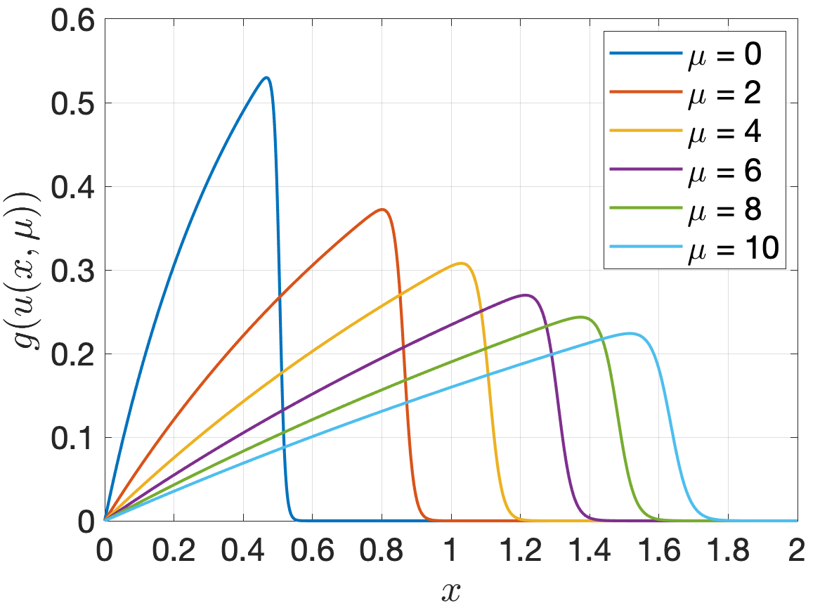
The test case involves the following parametrized functions
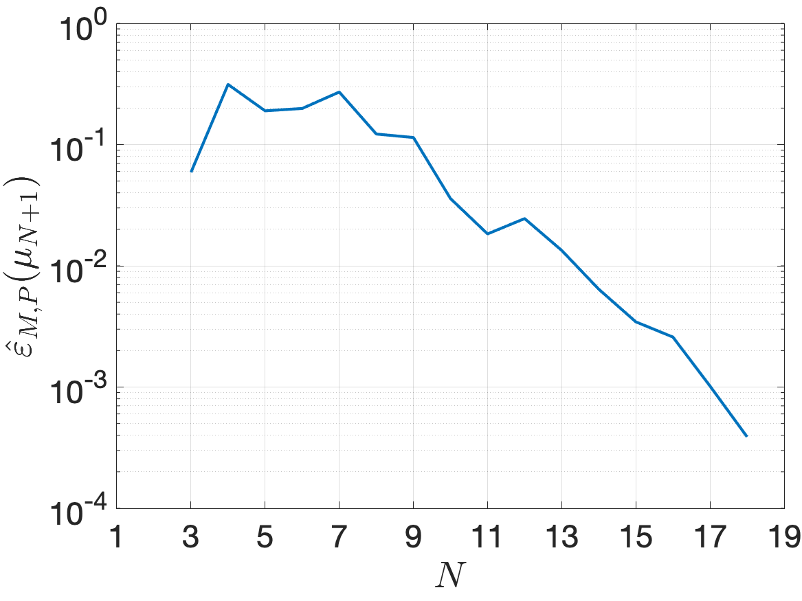
in a physical domain and parameter domain . Figure 1 shows the plots of the nonlinear function for different values of . For the greedy sampling method, we choose an initial sample and use a training sample of 100 parameter points distributed uniformly in the parameter space. The greedy algorithm iteratively selects new parameter points based on error estimates and stops when the maximum error estimate falls below the prescribed tolerance of . The error estimates of SOEIM with and are used to guide the greedy sampling. In this case, convergence is achieved at . Figure 1 demonstrates the decreasing trend of as increases, illustrating the effectiveness of the greedy sampling. The parameter points selected by the greedy sampling algorithm are listed in Table 1. These points are notably clustered toward the left side of the parameter space, indicating that this region requires a denser sampling to accurately capture the parametric manifold.
| 4 | 0.4040 | 8 | 1.6162 | 12 | 0.2020 | 16 | 8.9899 |
| 5 | 0.9091 | 9 | 7.9798 | 13 | 1.2121 | 17 | 5.6566 |
| 6 | 6.5657 | 10 | 2.1212 | 14 | 0.6061 | 18 | 3.4343 |
| 7 | 3.0303 | 11 | 3.9394 | 15 | 2.4242 | 19 | 4.3434 |
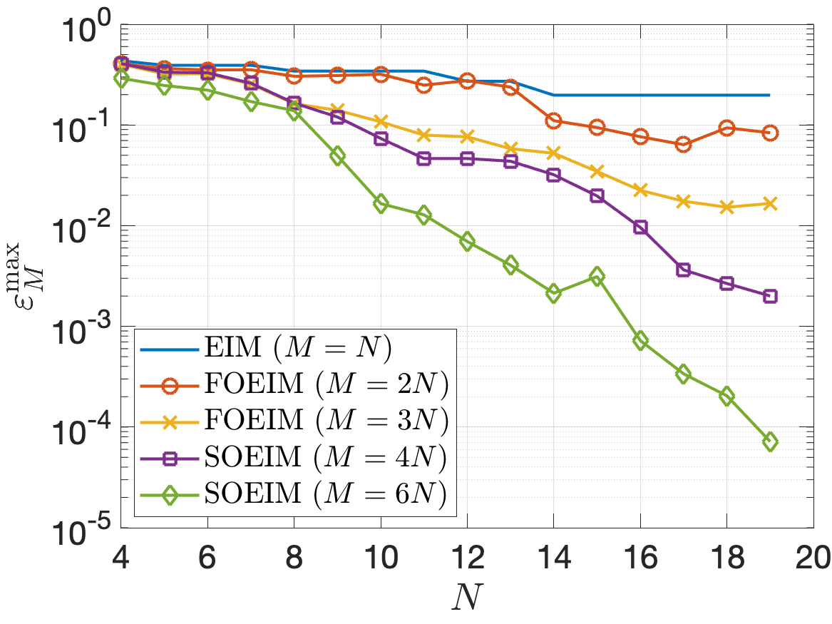
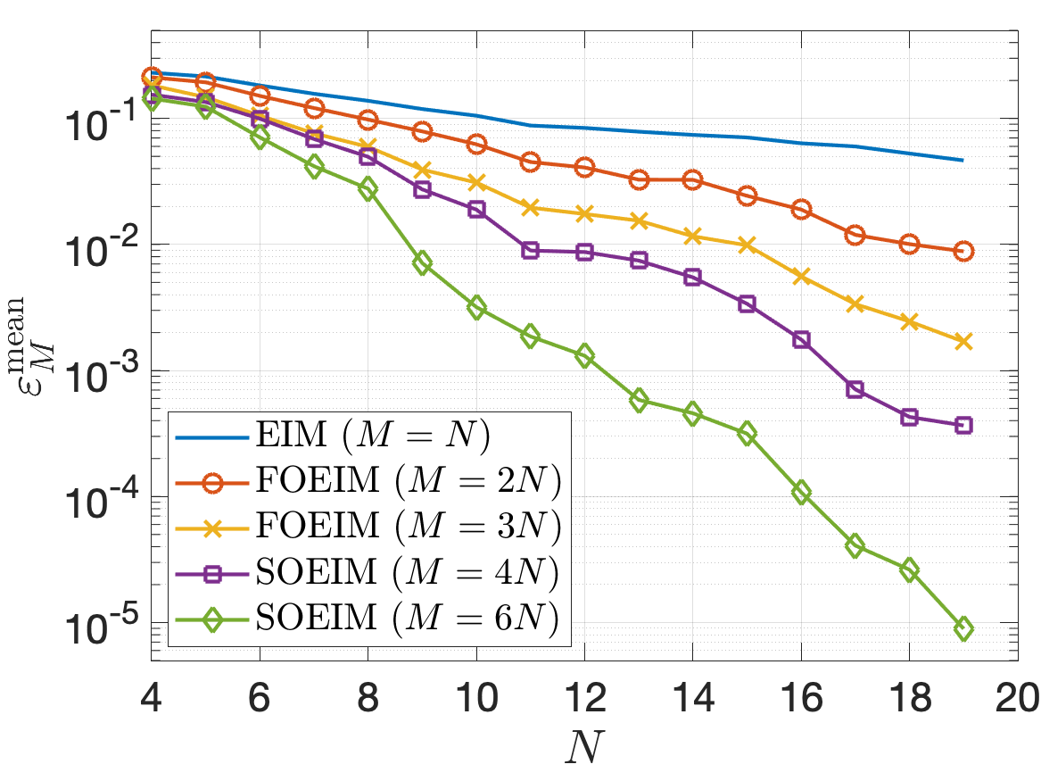
We use a test sample of parameter points distributed uniformly in the parameter space. The maximum error is defined as and the mean error as , where represents the interpolation error. Figure 2 plots and as a function of for EIM, FOEIM, and SOEIM. These plots illustrate how each method performs in reducing both the worst-case and average errors as increases. Both FOEIM and SOEIM exhibit superior error reduction compared to EIM, with SOEIM showing errors several orders of magnitude lower than EIM. We define the mean error estimate as and the mean effectivity as . Tables 2 and 3 present the values of and as a function and for FOEIM and SOEIM, respectively. The results indicate that the error estimates decrease rapidly as both and increase. Additionally, the error estimates are highly accurate, as reflected by the mean effectivities being consistently less than 5. This demonstrates that the estimation method provides sharp bounds on the actual error, ensuring efficiency, accuracy and reliability in the interpolation.
| 4 | 1.64e-1 | 0.86 | 3.53e-1 | 1.61 | 3.16e-1 | 1.86 |
|---|---|---|---|---|---|---|
| 7 | 1.72e-1 | 1.43 | 1.92e-1 | 1.47 | 7.93e-2 | 1.42 |
| 10 | 1.68e-1 | 2.05 | 9.42e-2 | 1.48 | 7.45e-2 | 2.68 |
| 13 | 1.50e-1 | 2.15 | 5.17e-2 | 1.84 | 3.44e-2 | 2.57 |
| 16 | 1.38e-1 | 2.88 | 4.34e-2 | 2.57 | 1.33e-2 | 2.89 |
| 19 | 1.07e-1 | 3.18 | 2.15e-2 | 2.83 | 7.23e-3 | 4.77 |
| 4 | 2.60e-1 | 1.19 | 1.13e-1 | 0.85 | 5.36e-2 | 0.45 |
|---|---|---|---|---|---|---|
| 7 | 1.40e-1 | 1.26 | 8.13e-2 | 1.41 | 6.05e-2 | 1.61 |
| 10 | 9.58e-2 | 1.62 | 2.44e-2 | 1.66 | 6.41e-3 | 2.12 |
| 13 | 8.28e-2 | 2.28 | 2.01e-2 | 3.03 | 1.64e-3 | 3.00 |
| 16 | 4.16e-2 | 2.11 | 4.28e-3 | 2.69 | 3.14e-4 | 2.95 |
| 19 | 2.23e-2 | 2.67 | 8.43e-4 | 2.67 | 2.74e-5 | 3.44 |
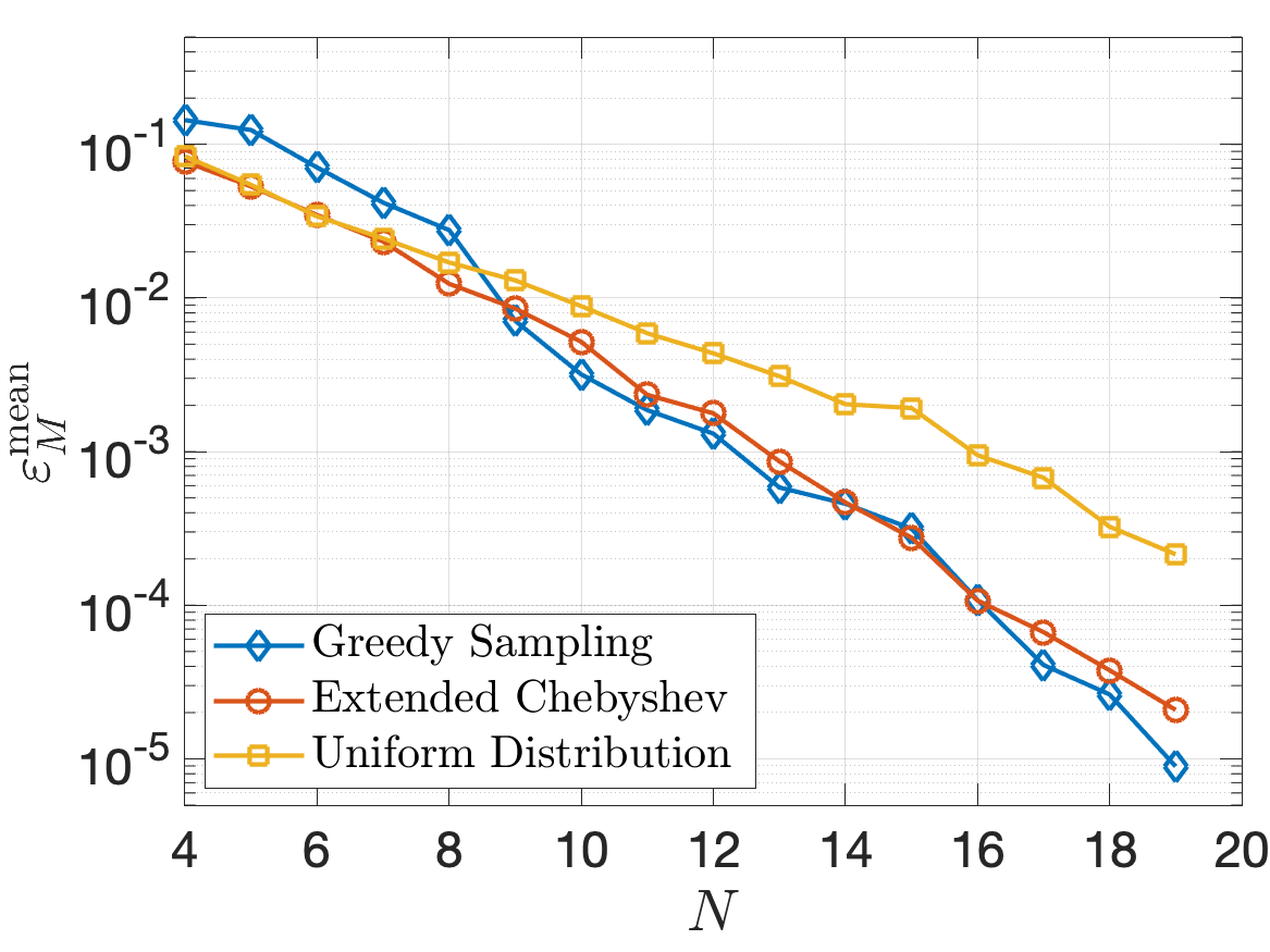
Figure 3 compares the convergence of the mean error as a function of for three sampling methods: Greedy Sampling, Extended Chebyshev, and Uniform Distribution. As increases, all methods demonstrate error reduction, with Greedy Sampling and Extended Chebyshev showing faster convergence and lower overall errors than Uniform Distribution. Greedy Sampling, in particular, exhibits superior performance at larger values of , indicating its ability to better capture important features with fewer parameter points. Uniform Distribution converges more slowly, yielding the highest errors at larger values of . A significant advantage of Greedy Sampling is its production of hierarchical samples, meaning new parameter points can be added incrementally to improve accuracy without reevaluating the entire set. This hierarchical nature makes Greedy Sampling highly flexible and efficient for ROM construction. In contrast, Extended Chebyshev, while competitive in terms of convergence rate, lacks the hierarchical refinement, limiting its adaptability.
4 Numerical results
In this section, we present numerical results from two parametrized nonlinear PDEs to assess and compare the performance of the H-GN and GN-H methods. Specifically, we investigate the impact of empirical interpolation methods on the convergence of these approaches relative to the standard GN method. For the H-GN method, we use three different interpolation methods – EIM, FOEIM, and SOEIM – to approximate the nonlinear terms, resulting in the EIM-GN, FOEIM-GN, and SOEIM-GN schemes, respectively. In the GN-H method, SOEIM is applied to nonlinear terms in the residual vector, while FOEIM is used for the Jacobian matrix, producing the GN-SOEIM scheme. To balance computational efficiency and accuracy, we set different values of for each method. For EIM-GN, we use , ensuring a basic level of approximation with the empirical interpolation method. For FOEIM-GN, is used to leverage first-order partial derivatives, enhancing the approximation. For SOEIM-GN, we increase to to incorporate second-order derivatives for more precise nonlinear term handling. In the GN-SOEIM method, we allocate for the residual vector and for the Jacobian matrix, allowing for higher accuracy in the residual while maintaining computational efficiency in the Jacobian approximation.
These methods are evaluated based on accuracy, computational cost, and convergence behavior. To assess the accuracy, we define the following errors
| (63) |
and the average errors
| (64) |
where is a test sample of parameter points distributed uniformly in the parameter domain. To measure the convergence of the H-GN and GN-H methods relative to the standard GN method, we define the effectivities
| (65) |
where and are the errors for the GN method. The average effectivities and are similarly defined.
4.1 A nonlinear elliptic problem
We consider the following parametrized nonlinear elliptic PDE
| (66) |
with homogeneous Dirichlet condition on the boundary , where and . The output of interest is the average of the field variable over the physical domain. The weak formulation is then stated as: given , find , where is the solution of
| (67) |
where
| (68) |
and
| (69) |
The finite element (FE) approximation space is , where is a space of polynomials of degree on an element and is a finite element grid of quadrilaterals. The dimension of the FE space is .
Figure 4 illustrates the parameter points selected via greedy sampling. The plot reveals that the majority of the points are concentrated along the boundary of the parameter domain, with a notable clustering near the top boundary. This distribution suggests that the regions near the boundary, particularly the upper edge, exhibit greater variability or complexity in the solution manifold, requiring more refined sampling. The greedy sampling algorithm effectively targets these areas to ensure better approximation accuracy while minimizing the number of points needed to capture the solution manifold. Figure 4 displays the interpolation points selected by the SOEIM method for parameter sample points. The interpolation points are well-distributed across the physical domain, ensuring good coverage for the interpolation. However, it is notable that only one of the interpolation points is located directly on the boundary of the physical domain. This can be attributed to the fact that the solution vanishes to zero along the boundary, making boundary points less critical for capturing the essential variation of the solution within the domain.
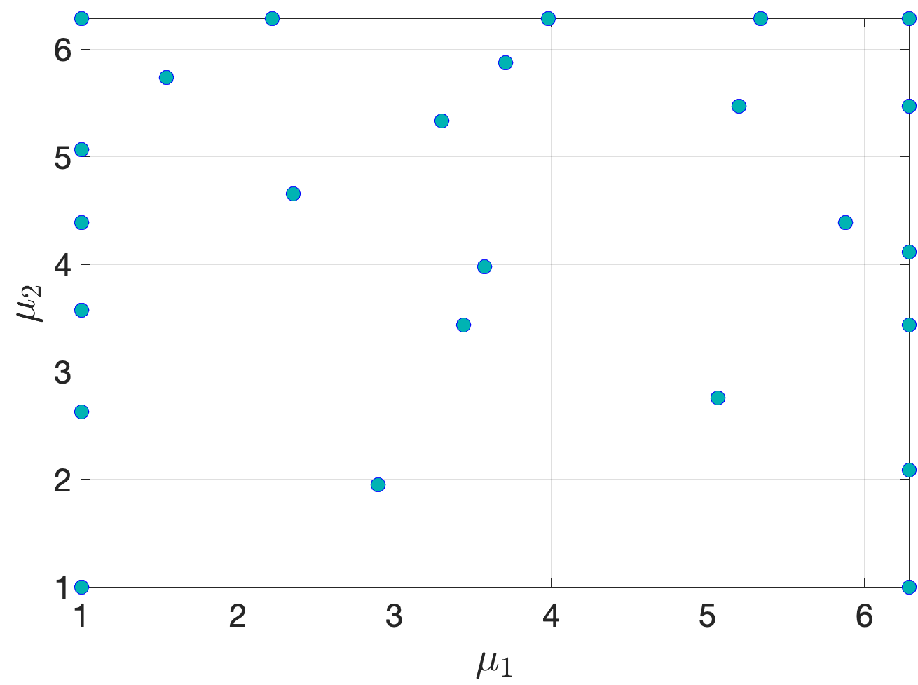
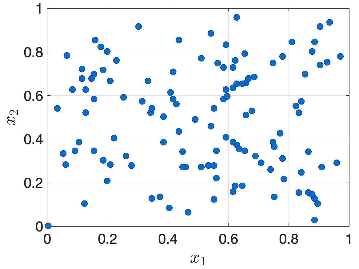
Figure 5 presents the convergence of the mean solution error and the mean output error as functions of for five methods: EIM-GN, FOEIM-GN, SOEIM-GN, GN-SOEIM, and the standard GN method. As increases, all methods exhibit a clear reduction in error. In particular, FOEIM-GN, SOEIM-GN, and GN-SOEIM converge significantly faster than EIM-GN. The GN-SOEIM method closely mirrors the accuracy of the standard GN method, becoming almost indistinguishable for values greater than 10. This demonstrates that high-order interpolation significantly improves convergence, approaching the full GN performance while maintaining computational efficiency.
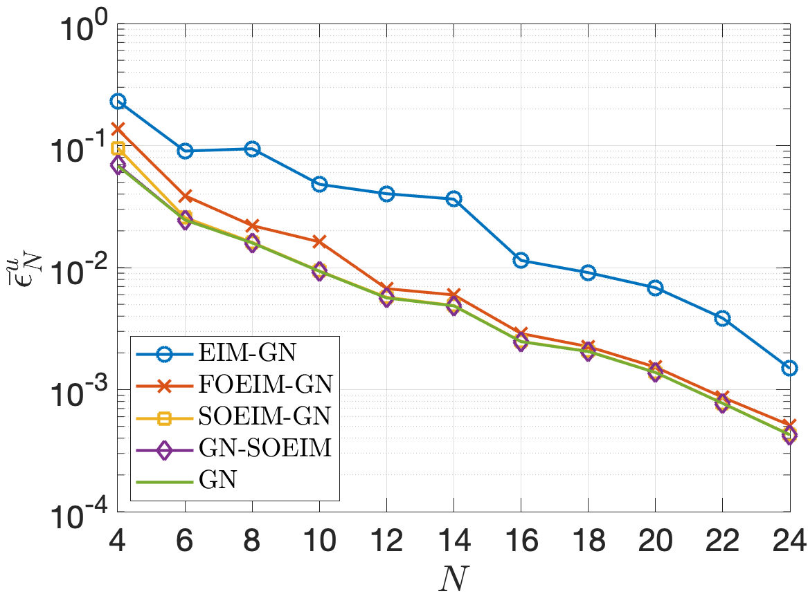
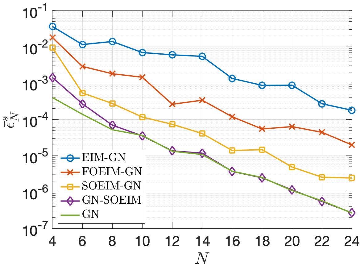
Table 4 presents the average effectivities (for the solution error) and (for the output error), as a function of for EIM-GN, FOEIM-GN, SOEIM-GN, and GN-SOEIM. Across all values of , GN-SOEIM consistently achieves the lowest effectivities. FOEIM-GN and SOEIM-GN perform significantly better than EIM-GN, especially as increases. For GN-SOEIM, the effectivities are very close to 1, indicating a very accurate and efficient approximation. In contrast, EIM-GN exhibits much larger effectivities, particularly in reaching values over 1000 for higher , demonstrating poorer performance in approximating the nonlinear terms. Notably, the output effectivties are considerably larger than the solution effectivities for EIM-GN, FOEIM-GN, and SOEIM-GN. This indicates that these methods struggle more with accurately approximating the output compared to the solution itself. Particularly in EIM-GN, the output effectivities grow substantially as increases. In contrast, GN-SOEIM maintains consistently low output effectivities, demonstrating superior accuracy in capturing both solution and output errors. This suggests that higher-order interpolation methods, especially GN-SOEIM, are far more effective in improving output approximations.
| EIM-GN | FOEIM-GN | SOEIM-GN | GN-SOEIM | |||||
|---|---|---|---|---|---|---|---|---|
| 4 | 3.12 | 206.41 | 1.98 | 66.9 | 1.27 | 42.04 | 1.01 | 3.72 |
| 6 | 4.02 | 325.04 | 2.03 | 63.95 | 1.06 | 6.49 | 1.00 | 1.51 |
| 8 | 6.15 | 550.4 | 1.68 | 69.24 | 1.02 | 8.28 | 1.00 | 1.21 |
| 10 | 5.44 | 490.66 | 2.03 | 75.66 | 1.02 | 6.94 | 1.00 | 1.22 |
| 12 | 7.51 | 835.83 | 1.36 | 45.09 | 1.03 | 8.89 | 1.00 | 1.11 |
| 14 | 7.04 | 777.49 | 1.54 | 59.95 | 1.03 | 6.25 | 1.00 | 1.26 |
| 16 | 5.04 | 660.79 | 1.36 | 67.44 | 1.02 | 6.49 | 1.00 | 1.14 |
| 18 | 4.90 | 607.98 | 1.34 | 55.63 | 1.03 | 8.05 | 1.00 | 1.03 |
| 20 | 5.19 | 1153.0 | 1.38 | 101.82 | 1.01 | 8.40 | 1.00 | 1.13 |
| 22 | 5.36 | 842.1 | 1.30 | 103.13 | 1.01 | 7.86 | 1.00 | 1.06 |
| 24 | 4.02 | 1165.94 | 1.55 | 97.63 | 1.02 | 9.00 | 1.00 | 1.17 |
Table 5 shows the computational speedup for various model reduction methods – GN, EIM-GN, FOEIM-GN, SOEIM-GN, and GN-SOEIM – compared to the finite element method (FEM) for different values of . Except for the standard GN method, the other model reduction methods provide substantial speedups relative to FEM. Across all values of , the GN method achieves a modest speedup (around 2.2–2.7x) compared to FEM. In contrast, the EIM-GN method provides the highest speedup, ranging from over 5000x at to about 2400x at , though its performance declines as increases. FOEIM-GN and SOEIM-GN demonstrate more consistent speedups (around 1700x–4200x), offering a good balance between computational efficiency and accuracy. GN-SOEIM maintains strong performance with speedup factors around 2000x–4600x. While both GN-SOEIM and FOEIM-GN exhibit similar speedup factors across a range of values for , GN-SOEIM consistently outperforms FOEIM-GN in terms of accuracy. This superior performance stems from GN-SOEIM’s use of second-order derivatives to approximate the residual and first-order derivatives for the Jacobian matrix, providing a more flexible hyperreduction strategy. The ability to balance these two interpolation techniques allows GN-SOEIM to effectively handle nonlinearities, offering a better trade-off between computational efficiency and accuracy.
| GN | EIM-GN | FOEIM-GN | SOEIM-GN | GN-SOEIM | |
|---|---|---|---|---|---|
| 4 | 2.52 | 5064.67 | 4258.1 | 3970.35 | 4601.2 |
| 6 | 2.73 | 4052.52 | 4163.69 | 3555.97 | 4239.4 |
| 8 | 2.76 | 3763.17 | 3938.08 | 3417.1 | 4480.89 |
| 10 | 2.73 | 3589.21 | 3561.61 | 3537.51 | 4064.43 |
| 12 | 2.66 | 3273.34 | 3467.02 | 3284.13 | 3813.88 |
| 14 | 2.48 | 3049.29 | 3117.96 | 2838.7 | 3419.49 |
| 16 | 2.40 | 3211.92 | 3011.17 | 2711.65 | 3390.79 |
| 18 | 2.18 | 2566.5 | 2385.51 | 2076.51 | 2630.22 |
| 20 | 2.26 | 2598.66 | 2412.79 | 2052.85 | 2391.55 |
| 22 | 2.24 | 2427.95 | 2208.71 | 1795.99 | 2217.08 |
| 24 | 2.27 | 2364.06 | 2122.91 | 1676.67 | 2070.6 |
4.2 A nonlinear convection-diffusion-reaction problem
We consider a nonlinear convection-diffusion-reaction problem
| (70) |
with homogeneous Dirichlet condition on . Here is a unit square domain, while is the parameter vector in a parameter domain . The reaction term is a nonlinear function of the state variable .
Let be a finite element (FE) approximation space of dimension with , where is a space of polynomials of degree on an element and is a finite element grid of quadrilaterals. The dimension of the FE space is . The FE approximation of the exact solution is the solution of
| (71) |
with being the nonlinear convection term. The output of interest is evaluated as with . Figure 6 shows four instances of corresponding to the four corners of the parameter domain.
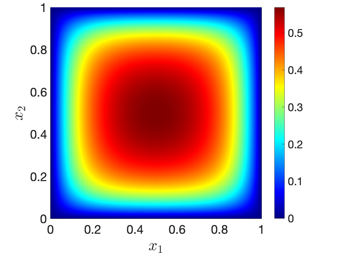
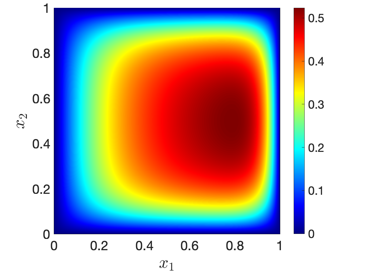
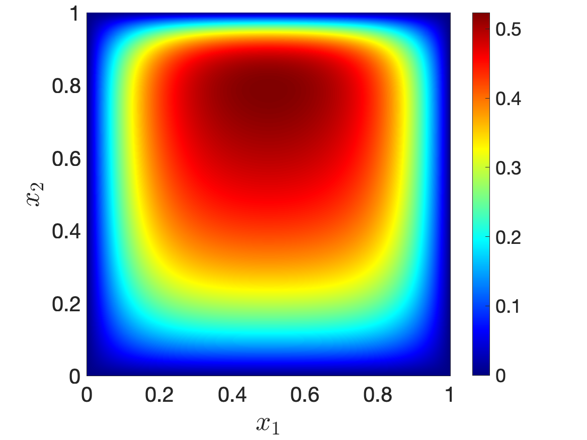
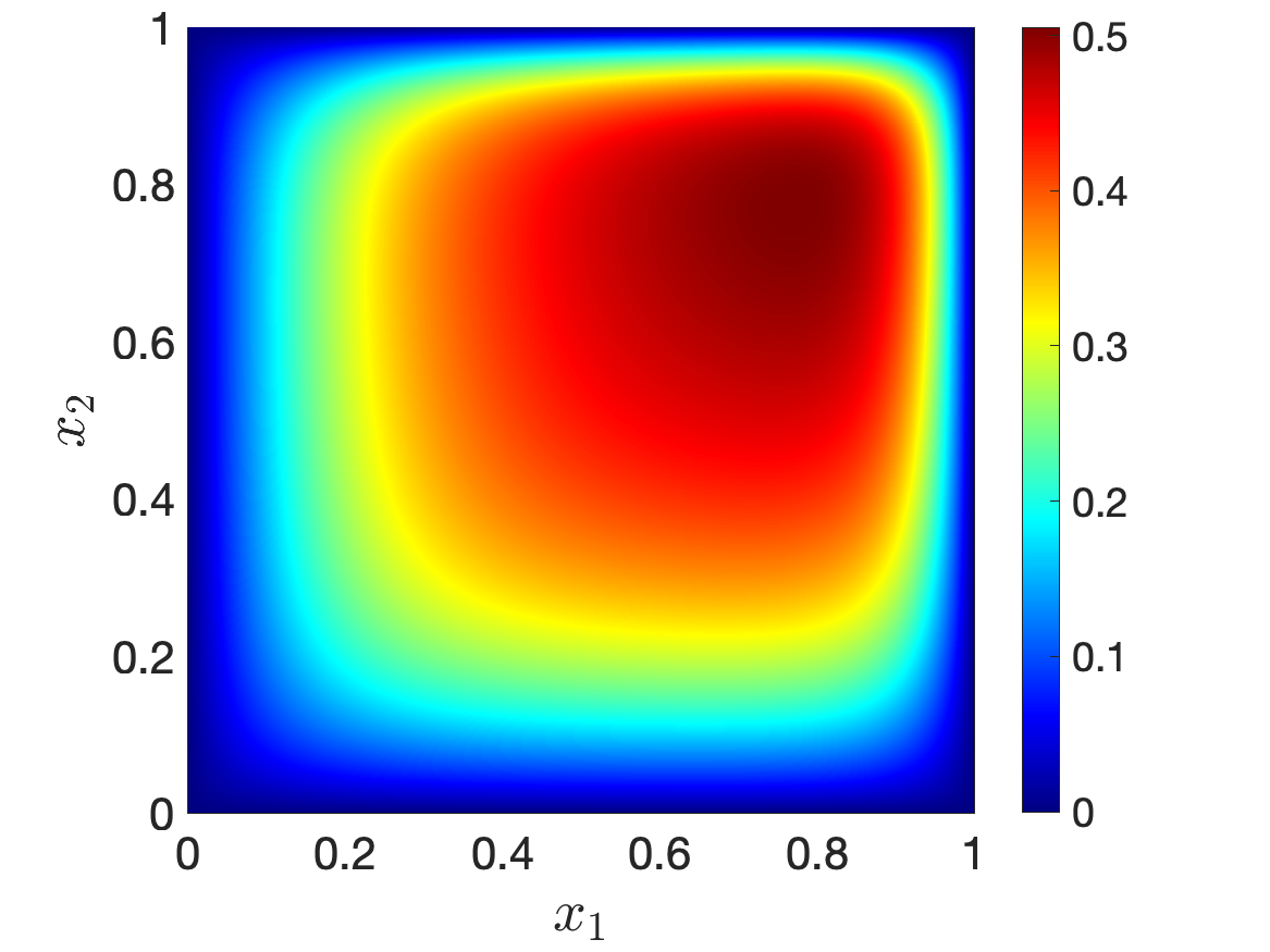
Figure 7 illustrates the parameter points selected via greedy sampling. The plot reveals that the majority of the points are concentrated along the boundary of the parameter domain. This distribution suggests that the regions near the boundary exhibit greater variability or complexity in the solution manifold, requiring more refined sampling. Figure 7 displays the interpolation points selected by the SOEIM method for parameter sample points. The interpolation points are well-distributed across the physical domain. However, it is notable that only none of the interpolation points is located directly on the boundary of the physical domain since the solution vanishes to zero along the boundary, making boundary points less critical for capturing the essential variation of the solution within the domain. Figure 8 presents the convergence of the mean solution error and the mean output error as functions of for five methods: EIM-GN, FOEIM-GN, SOEIM-GN, GN-SOEIM, and the standard GN method. As increases, all methods tend to reduce the errors. The accuracy of the GN-SOEIM method is almost indistinguishable from that of the standard GN method. This demonstrates that high-order interpolation significantly improves convergence, approaching the full GN performance while maintaining computational efficiency.
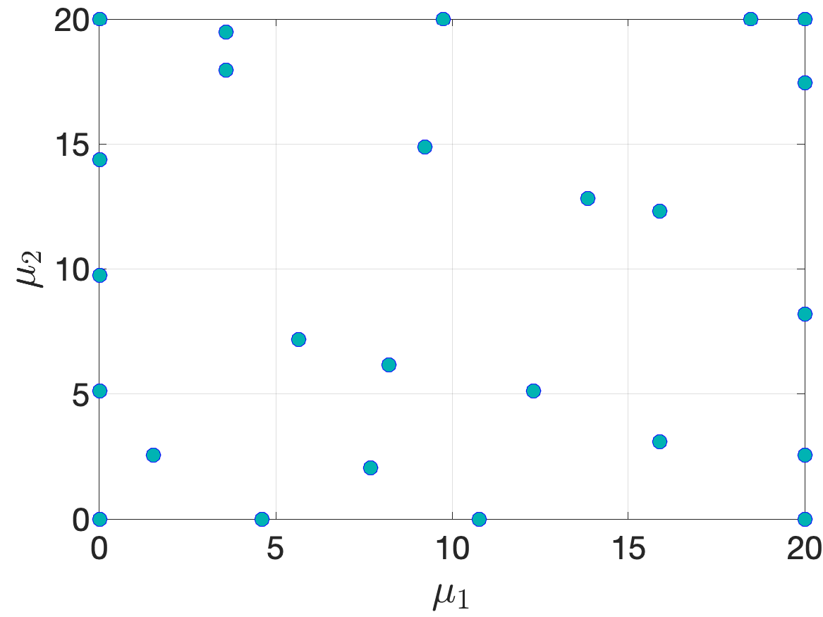
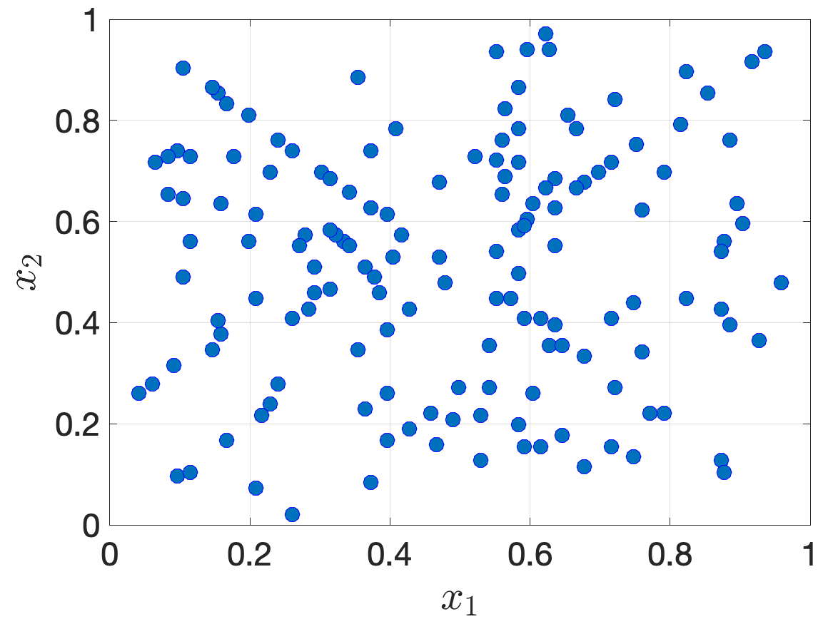
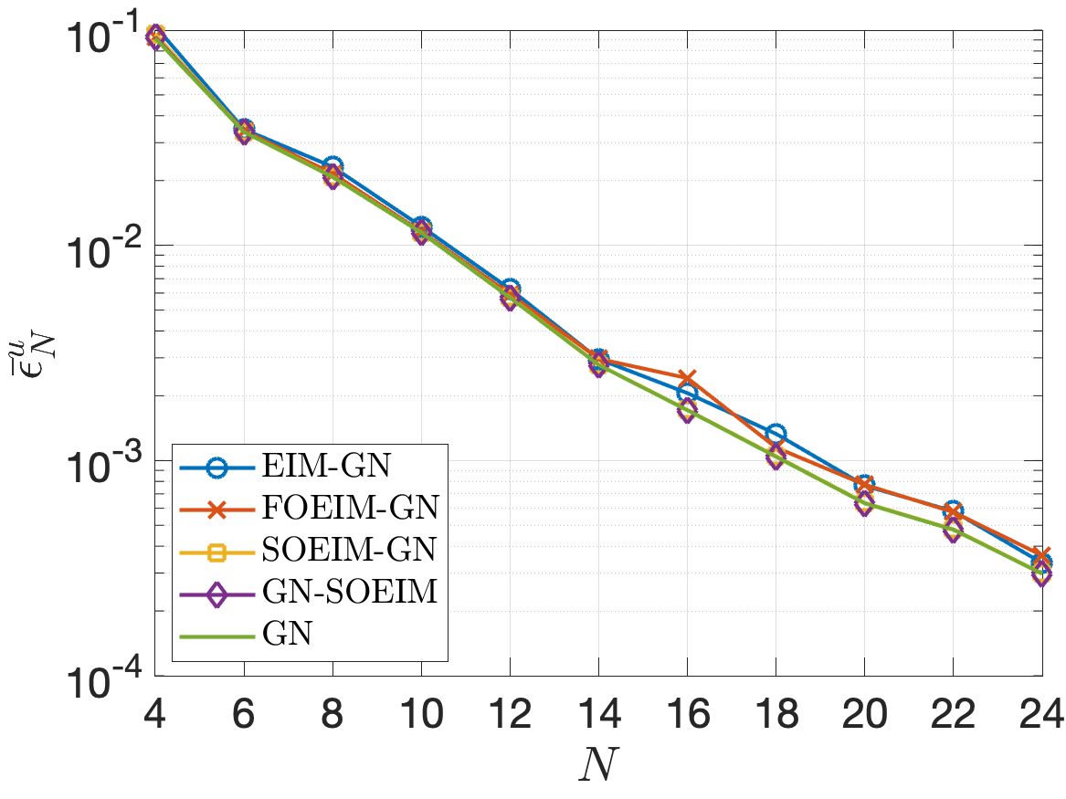
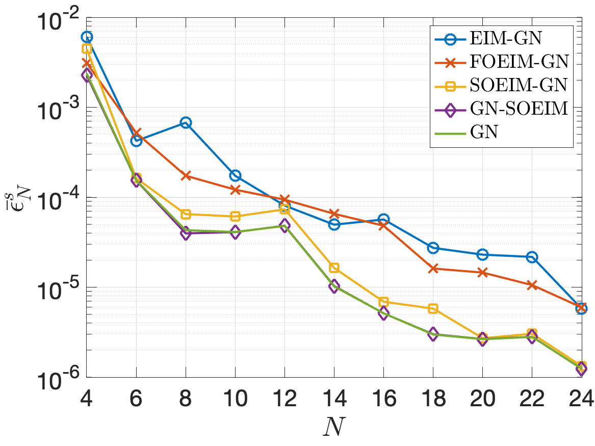
Table 6 presents and , as a function of for EIM-GN, FOEIM-GN, SOEIM-GN, and GN-SOEIM. SOEIM-GN performs better than both EIM-GN and FOEIM-GN. Across all values of , GN-SOEIM consistently achieves the lowest effectivities very close to 1, indicating a very accurate and efficient approximation. Notably, the output effectivties are considerably larger than the solution effectivities for EIM-GN and FOEIM-GN. In contrast, GN-SOEIM maintains consistently low output effectivities. Table 7 shows the computational speedup for various model reduction methods – GN, EIM-GN, FOEIM-GN, SOEIM-GN, and GN-SOEIM – compared to the finite element method (FEM) for different values of . Except for the standard GN method, the other model reduction methods provide substantial speedups relative to FEM. Across all values of , the GN method achieves a modest speedup (around 2.3–3.0x) compared to FEM. In contrast, the EIM-GN method provides the highest speedup over 5000x. While GN-SOEIM exhibits similar speedup factors across a range of values for (around 5000x–7000x), it consistently outperforms other methods in terms of accuracy. This superior performance highlights the flexibility of GN-SOEIM in balancing computational efficiency and accuracy.
| EIM-GN | FOEIM-GN | SOEIM-GN | GN-SOEIM | |||||
|---|---|---|---|---|---|---|---|---|
| 4 | 1.13 | 2.60 | 1.02 | 1.33 | 1.04 | 2.05 | 1.01 | 0.97 |
| 6 | 1.03 | 18.80 | 1.05 | 15.37 | 1.00 | 1.88 | 1.00 | 1.02 |
| 8 | 1.32 | 28.15 | 1.10 | 10.78 | 1.01 | 3.38 | 1.00 | 0.99 |
| 10 | 1.07 | 16.79 | 1.08 | 9.78 | 1.01 | 2.55 | 1.00 | 1.02 |
| 12 | 1.10 | 10.65 | 1.12 | 6.67 | 1.02 | 3.21 | 1.00 | 1.02 |
| 14 | 1.08 | 13.89 | 1.22 | 17.13 | 1.01 | 2.68 | 1.00 | 1.04 |
| 16 | 1.22 | 43.72 | 1.84 | 24.98 | 1.01 | 2.37 | 1.00 | 1.01 |
| 18 | 1.29 | 20.50 | 1.38 | 16.35 | 1.05 | 3.45 | 1.00 | 1.02 |
| 20 | 1.23 | 31.65 | 1.68 | 19.02 | 1.05 | 2.18 | 1.00 | 1.01 |
| 22 | 1.27 | 24.70 | 1.61 | 15.92 | 1.03 | 1.54 | 1.00 | 1.01 |
| 24 | 1.14 | 21.92 | 1.55 | 16.16 | 1.02 | 1.61 | 1.00 | 1.02 |
| GN | EIM-GN | FOEIM-GN | SOEIM-GN | GN-SOEIM | |
|---|---|---|---|---|---|
| 4 | 2.94 | 7845.03 | 6865.92 | 5708.78 | 6982.76 |
| 6 | 2.76 | 6933.33 | 6614.44 | 5268.42 | 6439.73 |
| 8 | 2.73 | 6864.69 | 6637.31 | 4876.92 | 6266.16 |
| 10 | 2.75 | 6607.40 | 6606.95 | 4633.53 | 6005.09 |
| 12 | 2.77 | 6308.04 | 6215.00 | 4525.95 | 5828.64 |
| 14 | 2.73 | 6183.81 | 6112.42 | 4392.77 | 5536.80 |
| 16 | 2.71 | 6125.53 | 6073.42 | 4132.52 | 5490.81 |
| 18 | 2.60 | 5971.05 | 5780.55 | 4061.84 | 5239.08 |
| 20 | 2.44 | 5863.68 | 5626.32 | 3828.42 | 5173.65 |
| 22 | 2.38 | 5739.28 | 5444.94 | 3772.29 | 5012.31 |
| 24 | 2.43 | 5663.73 | 5354.86 | 3662.05 | 4977.26 |
5 Conclusions
This paper presents a class of high-order empirical interpolation methods to develop reduced-order models for parametrized nonlinear PDEs. The proposed methods significantly enhance the approximation power by leveraging higher-order partial derivatives to construct additional basis functions and interpolation points, providing greater accuracy and efficiency in reducing the dimensionality of nonlinear PDEs. Through numerical experiments, we demonstrated the superior convergence and accuracy of the high-order methods compared to traditional model reduction methods. These results suggest that the proposed methods can be widely applicable to a variety of problems, including those involving nonlinearities and nonaffine structures, while maintaining computational efficiency. Future work will focus on extending these methods to other nonlinear and time-dependent systems, as well as investigating their applicability to real-time control and optimization in engineering applications.
The development of model reduction methods is a very active area of research filled with open questions concerning the stability, accuracy, efficiency, and robustness of the reduced models. Model reduction methods can produce unstable or inaccurate solutions if they fail to preserve the geometric structures of the full model, such as conservation laws, symmetries, and invariants. To address this issue, structure-preserving model reduction techniques [60, 61, 62, 63, 64, 65, 66, 67, 68] ensure that reduced models maintain key properties to improve both stability and accuracy. While hyper-reduction methods have successfully created efficient low-dimensional models, few approaches retain the structure of nonlinear operators such as the symplectic DEIM [69] and energy-conserving ECSW scheme [39]. We would like to extend the high-order EIM to preserve geometric structures of the full model.
Model reduction on nonlinear manifolds was originated with the work [70] on reduced-order modeling of nonlinear structural dynamics using quadratic manifolds. This concept was further extended through the use of deep convolutional autoencoders by Lee and Carlberg [71]. Recently, quadratic manifolds are further developed to address the challenges posed by the Kolmogorov barrier in model order reduction [72, 73]. Another approach is model reduction through lifting or variable transformations, as demonstrated by Kramer and Willcox [49], where nonlinear systems are reformulated in a quadratic framework, making the reduced model more tractable. This method was expanded in the ”Lift & Learn” framework [74] and operator inference techniques [75, 76], leveraging physics-informed machine learning for large-scale nonlinear dynamical systems. We will combine our approach with nonlinear manifolds to develop more efficient ROMs for nonlinear PDEs.
Model reduction methods applied to convection-dominated problems often struggle due to slowly decaying Kolmogorov widths caused by moving shocks and discontinuities. To address this issue, various techniques recast the problem in a more suitable coordinate frame using parameter-dependent maps, improving convergence. Approaches include POD-Galerkin methods with shifted reference frames [77], optimal transport methods [78, 79, 80], and phase decomposition. Recent methods like shifted POD [81], transport reversal [82], and transport snapshot [83] use time-dependent shifts, while registration [84] and shock-fitting methods [85, 86] minimize residuals to determine the map for better low-dimensional representations. We would like to extend this work to convection-dominated problems based on the optimal transport [79, 80].
With advances in data analytics and machine learning, data-driven ROMs have gained significant attention. Unlike projection-based ROMs, which rely on mathematical operators for Galerkin projection, data-driven ROMs infer expansion coefficients using regression models like radial basis functions [87, 88, 79, 89, 90], Gaussian processes [91, 92, 93], or neural networks [94, 95, 96]. These models treat the full-order model as a black box, making them easier to implement. However, they often lack error certification and require a large number of snapshots, which can be expensive for complex, high-dimensional systems. Future research will extend the proposed approach to data-driven model reduction.
A posteriori error estimation provides a critical advantage by ensuring confidence in the reduced model’s accuracy and guiding the selection of the reduced model size based on accuracy needs. While rigorous error estimation techniques are well-developed for linear and weakly nonlinear PDEs [2, 4, 6, 7, 8, 9, 10, 11, 12, 13, 14, 16, 1, 17, 18, 19, 20], highly nonlinear PDEs present significant challenges. Dual-weighted residual (DWR) method enables error estimation in model reduction by using adjoint solutions to tailor error estimates for specific outputs [97, 14, 1, 98, 99, 100, 101, 102]. While DWR enhances reduced-order model (ROM) accuracy, it requires solving adjoint problems and is limited to first-order accuracy. To overcome these limitations, machine-learning error models [103, 104] employ neural networks to predict errors. These models are more flexible but DWR remains more reliable for out-of-distribution errors. Future work will leverage these approaches to develop practical and reliable error estimates.
Acknowledgements
I would like to thank Professors Jaime Peraire, Anthony T. Patera, and Robert M. Freund at MIT, and Professor Yvon Maday at University of Paris VI for fruitful discussions. I gratefully acknowledge a Seed Grant from the MIT Portugal Program, the United States Department of Energy under contract DE-NA0003965 and the Air Force Office of Scientific Research under Grant No. FA9550-22-1-0356 for supporting this work.
References
-
[1]
G. Rozza, D. B. P. Huynh, A. T. Patera, Reduced basis approximation and a posteriori error estimation for affinely parametrized elliptic coercive partial differential equations: Application to transport and continuum mechanics, Archives Computational Methods in Engineering 15 (3) (2008) 229–275.
doi:10.1007/s11831-008-9019-9.
URL http://link.springer.com/10.1007/s11831-008-9019-9 - [2] Y. Chen, J. S. Hesthaven, Y. Maday, J. Rodríguez, Improved successive constraint method based a posteriori error estimate for reduced basis approximation of 2D Maxwell’s problem, ESAIM - Mathematical Modelling and Numerical Analysis 43 (6) (2009) 1099–1116. doi:10.1051/m2an/2009037.
-
[3]
Y. Chen, J. S. Hesthaven, Y. Maday, J. Rodríguez, Certified Reduced Basis Methods and Output Bounds for the Harmonic Maxwell’s Equations, SIAM Journal on Scientific Computing 32 (2) (2010) 970–996.
doi:10.1137/09075250X.
URL http://epubs.siam.org/action/showAbstract?page=970{&}volume=32{&}issue=2{&}journalCode=sjoce3 - [4] S. Deparis, Reduced basis error bound computation of parameter-dependent Navier-stokes equations by the natural norm approach, SIAM Journal on Numerical Analysis 46 (4) (2008) 2039–2067. doi:10.1137/060674181.
- [5] J. Eftang, A. Patera, E. Ronquist, An ”hp” Certified Reduced Basis Method for Parametrized Elliptic Partial Differential Equations, SIAM Journal on Scientific Computing 32 (6) (2010) 3170–3200.
- [6] J. L. Eftang, D. B. Huynh, D. J. Knezevic, A. T. Patera, A two-step certified reduced basis method, Journal of Scientific Computing 51 (1) (2012) 28–58. doi:10.1007/s10915-011-9494-2.
- [7] D. B. Huynh, A. T. Patera, Reduced basis approximation and a posteriori error estimation for stress intensity factors, International Journal for Numerical Methods in Engineering 72 (10) (2007) 1219–1259. doi:10.1002/nme.2090.
-
[8]
D. Huynh, D. Knezevic, Y. Chen, J. Hesthaven, A. Patera, A natural-norm Successive Constraint Method for inf-sup lower bounds, Computer Methods in Applied Mechanics and Engineering 199 (29-32) (2010) 1963–1975.
doi:10.1016/j.cma.2010.02.011.
URL http://dx.doi.org/10.1016/j.cma.2010.02.011 - [9] D. B. P. Huynh, D. J. Knezevic, A. T. Patera, A Static condensation Reduced Basis Element method : Approximation and a posteriori error estimation, Mathematical Modelling and Numerical Analysis 47 (1) (2013) 213–251. doi:10.1051/m2an/2012022.
- [10] M. Kärcher, Z. Tokoutsi, M. A. Grepl, K. Veroy, Certified Reduced Basis Methods for Parametrized Elliptic Optimal Control Problems with Distributed Controls, Journal of Scientific Computing 75 (1) (2018) 276–307. doi:10.1007/s10915-017-0539-z.
- [11] D. J. Knezevic, N. C. Nguyen, A. T. Patera, Reduced basis approximation and a posteriori error estimation for the parametrized unsteady Boussinesq equations, Mathematical Models and Methods in Applied Sciences 21 (7) (2011) 1415–1442. doi:10.1142/S0218202511005441.
- [12] D. J. Knezevic, A. T. Patera, A certified reduced basis method for the fokker-planck equation of dilute polymeric fluids: Fene dumbbells in extensional flow, SIAM Journal on Scientific Computing 32 (2) (2010) 793–817. doi:10.1137/090759239.
- [13] N. C. Nguyen, K. Veroy, A. T. Patera, Certified Real-Time Solution of Parametrized Partial Differential Equations, in: S. Yip (Ed.), Handbook of Materials Modeling, Kluwer Academic Publishing, 2004, pp. 1523–1559.
-
[14]
N. C. Nguyen, A posteriori error estimation and basis adaptivity for reduced-basis approximation of nonaffine-parametrized linear elliptic partial differential equations, Journal of Computational Physics 227 (2) (2007) 983–1006.
doi:10.1016/j.jcp.2007.08.031.
URL http://linkinghub.elsevier.com/retrieve/pii/S0021999107003749 - [15] N. C. Nguyen, G. Rozza, D. B. P. Huynh, A. T. Patera, Reduced Basis Approximation and A Posteriori Error Estimation for Parametrized Parabolic PDEs; Application to Real-Time Bayesian Parameter Estimation, in: Biegler, Biros, Ghattas, Heinkenschloss, Keyes, Mallick, Tenorio, van Bloemen Waanders, Willcox (Eds.), Computational Methods for Large Scale Inverse Problems and Uncertainty Quantification, John Wiley and Sons, UK, 2010.
-
[16]
N. C. Nguyen, G. Rozza, A. T. Patera, Reduced basis approximation and a posteriori error estimation for the time-dependent viscous Burgers’ equation, Calcolo 46 (3) (2009) 157–185.
doi:10.1007/s10092-009-0005-x.
URL http://link.springer.com/10.1007/s10092-009-0005-x - [17] G. Rozza, Reduced-basis methods for elliptic equations in sub-domains with {em a posteriori/} error bounds and adaptivity, Appl. Numer. Math. 55 (4) (2005) 403–424.
- [18] S. Sen, K. Veroy, D. B. Huynh, S. Deparis, N. C. Nguyen, A. T. Patera, ”Natural norm” a posteriori error estimators for reduced basis approximations, Journal of Computational Physics 217 (1) (2006) 37–62. doi:10.1016/j.jcp.2006.02.012.
- [19] K. Veroy, A. T. Patera, Certified real-time solution of the parametrized steady incompressible Navier-Stokes equations: Rigorous reduced-basis a posteriori error bounds, International Journal for Numerical Methods in Fluids 47 (8-9) (2005) 773–788. doi:10.1002/fld.867.
- [20] K. Veroy, D. V. Rovas, A. T. Patera, A posteriori error estimation for reduced-basis approximation of parametrized elliptic coercive partial differential equations: ”Convex inverse” bound conditioners, ESAIM - Control, Optimisation and Calculus of Variations 8 (2002) 1007–1028. doi:10.1051/cocv:2002041.
- [21] F. Vidal-Codina, N. C. Nguyen, M. B. Giles, J. Peraire, A model and variance reduction method for computing statistical outputs of stochastic elliptic partial differential equations, Journal of Computational Physics 297 (2015) 700–720. arXiv:1409.1526, doi:10.1016/j.jcp.2015.05.041.
- [22] F. Vidal-Codina, N. C. Nguyen, J. Peraire, Computing parametrized solutions for plasmonic nanogap structures, Journal of Computational Physics 366 (2018) 89–106. arXiv:1710.06539, doi:10.1016/j.jcp.2018.04.009.
-
[23]
M. Barrault, Y. Maday, N. C. Nguyen, A. T. Patera, An ’empirical interpolation’ method: application to efficient reduced-basis discretization of partial differential equations, Comptes Rendus Mathematique 339 (9) (2004) 667–672.
doi:10.1016/J.Crma.2004.08.006.
URL http://www.sciencedirect.com/science/article/pii/S1631073X04004248http://linkinghub.elsevier.com/retrieve/pii/S1631073X04004248 -
[24]
M. A. Grepl, Y. Maday, N. C. Nguyen, A. T. Patera, Efficient reduced-basis treatment of nonaffine and nonlinear partial differential equations, Mathematical Modelling and Numerical Analysis 41 (3) (2007) 575–605.
doi:10.1051/m2an:2007031.
URL http://www.esaim-m2an.org/10.1051/m2an:2007031http://journals.cambridge.org/abstract{_}S0764583X07000313 - [25] M. Drohmann, B. Haasdonk, M. Ohlberger, Reduced basis approximation for nonlinear parametrized evolution equations based on empirical operator interpolation, SIAM Journal on Scientific Computing 34 (2) (2012) A937–A969. doi:10.1137/10081157X.
- [26] A. Manzoni, A. Quarteroni, G. Rozza, Shape optimization for viscous flows by reduced basis methods and free-form deformation, International Journal for Numerical Methods in Fluids 70 (5) (2012) 646–670. doi:10.1002/fld.2712.
- [27] J. S. Hesthaven, B. Stamm, S. Zhang, Efficient greedy algorithms for high-dimensional parameter spaces with applications to empirical interpolation and reduced basis methods, ESAIM: Mathematical Modelling and Numerical Analysis 48 (1) (2014) 259–283. doi:10.1051/m2an/2013100.
- [28] J. S. Hesthaven, C. Pagliantini, G. Rozza, Reduced basis methods for time-dependent problems, Acta Numerica 31 (2022) 265–345. doi:10.1017/S0962492922000058.
- [29] Y. Chen, S. Gottlieb, L. Ji, Y. Maday, An EIM-degradation free reduced basis method via over collocation and residual hyper reduction-based error estimation, Journal of Computational Physics 444 (2021) 110545. doi:10.1016/j.jcp.2021.110545.
- [30] J. L. Eftang, M. A. Grepl, A. T. Patera, A posteriori error bounds for the empirical interpolation method, Comptes Rendus Mathematique 348 (9-10) (2010) 575–579. doi:10.1016/j.crma.2010.03.004.
-
[31]
N. C. Nguyen, A. T. Patera, J. Peraire, A ’best points’ interpolation method for efficient approximation of parametrized functions, International Journal for Numerical Methods in Engineering 73 (4) (2008) 521–543.
doi:10.1002/nme.2086.
URL http://doi.wiley.com/10.1002/nme.2086 -
[32]
N. C. Nguyen, J. Peraire, N.~C.~Nguyen, J.~Peraire, An efficient reduced-order modeling approach for non-linear parametrized partial differential equations, International Journal for Numerical Methods in Engineering 76 (1) (2008) 27–55.
doi:10.1002/nme.2309.
URL http://doi.wiley.com/10.1002/nme.2309 - [33] Y. Maday, O. Mula, A. T. Patera, M. Yano, The Generalized Empirical Interpolation Method: Stability theory on Hilbert spaces with an application to the Stokes equation, Computer Methods in Applied Mechanics and Engineering 287 (2015) 310–334. doi:10.1016/j.cma.2015.01.018.
- [34] Y. Maday, O. Mula, A generalized empirical interpolation method: Application of reduced basis techniques to data assimilation, in: Springer INdAM Series, Vol. 4, Springer, 2013, pp. 221–235. arXiv:1512.00683, doi:10.1007/978-88-470-2592-9-13.
- [35] A. T. Patera, M. Yano, Une procédure de quadrature empirique par programmation linéaire pour les fonctions à paramètres, Comptes Rendus Mathematique 355 (11) (2017) 1161–1167. doi:10.1016/j.crma.2017.10.020.
- [36] J. A. Hernández, M. A. Caicedo, A. Ferrer, Dimensional hyper-reduction of nonlinear finite element models via empirical cubature, Computer Methods in Applied Mechanics and Engineering 313 (2017) 687–722. doi:10.1016/j.cma.2016.10.022.
- [37] M. Yano, A. T. Patera, An LP empirical quadrature procedure for reduced basis treatment of parametrized nonlinear PDEs, Computer Methods in Applied Mechanics and Engineering 344 (2019) 1104–1123. doi:10.1016/j.cma.2018.02.028.
- [38] C. Farhat, P. Avery, T. Chapman, J. Cortial, Dimensional reduction of nonlinear finite element dynamic models with finite rotations and energy-based mesh sampling and weighting for computational efficiency, International Journal for Numerical Methods in Engineering 98 (9) (2014) 625–662. doi:10.1002/nme.4668.
- [39] C. Farhat, T. Chapman, P. Avery, Structure-preserving, stability, and accuracy properties of the energy-conserving sampling and weighting method for the hyper reduction of nonlinear finite element dynamic models, International Journal for Numerical Methods in Engineering 102 (5) (2015) 1077–1110. doi:10.1002/nme.4820.
- [40] R. Everson, L. Sirovich, Karhunen-Loeve procedure for gappy data, Opt. Soc. Am. A 12 (8) (1995) 1657–1664.
- [41] D. Galbally, K. Fidkowski, K. Willcox, O. Ghattas, Non-linear model reduction for uncertainty quantification in large-scale inverse problems, International Journal for Numerical Methods in Engineering 81 (12) (2010) 1581–1608. doi:10.1002/nme.2746.
- [42] K. Carlberg, C. Bou-Mosleh, C. Farhat, Efficient non-linear model reduction via a least-squares Petrov-Galerkin projection and compressive tensor approximations, International Journal for Numerical Methods in Engineering 86 (2) (2011) 155–181. doi:10.1002/nme.3050.
- [43] S. Chaturantabut, D. C. Sorensen, Application of POD and DEIM on dimension reduction of non-linear miscible viscous fingering in porous media, Mathematical and Computer Modelling of Dynamical Systems 17 (4) (2011) 337–353. doi:10.1080/13873954.2011.547660.
- [44] P. Kerfriden, O. Goury, T. Rabczuk, S. P. Bordas, A partitioned model order reduction approach to rationalise computational expenses in nonlinear fracture mechanics, Computer Methods in Applied Mechanics and Engineering 256 (2013) 169–188. arXiv:1208.3940, doi:10.1016/j.cma.2012.12.004.
- [45] A. Radermacher, S. Reese, POD-based model reduction with empirical interpolation applied to nonlinear elasticity, International Journal for Numerical Methods in Engineering 107 (6) (2016) 477–495. doi:10.1002/nme.5177.
-
[46]
N. C. Nguyen, J. Peraire, Efficient and accurate nonlinear model reduction via first-order empirical interpolation, Journal of Computational Physics 494 (2023) 112512.
arXiv:2305.00466, doi:10.1016/j.jcp.2023.112512.
URL http://arxiv.org/abs/2305.00466 -
[47]
N. C. Nguyen, Model reduction techniques for parametrized nonlinear partial differential equations, in: Advances in Applied Mechanics, Vol. 58, Elsevier, 2024, pp. 135–190.
doi:10.1016/bs.aams.2024.03.005.
URL https://www.sciencedirect.com/science/article/pii/S0065215624000073 -
[48]
Y. Maday, N. C. Nguyen, A. T. Patera, S. Pau, G. S. H. Pau, A general, multipurpose interpolation procedure: the magic points., Communications on Pure and Applied Analysis 8 (1) (2009) 383–404.
doi:10.3934/cpaa.2009.8.383.
URL http://www.aimsciences.org/journals/displayArticles.jsp?paperID=3753 - [49] B. Kramer, K. E. Willcox, Nonlinear model order reduction via lifting transformations and proper orthogonal decomposition, AIAA Journal 57 (6) (2019) 2297–2307. arXiv:1808.02086, doi:10.2514/1.J057791.
- [50] B. Peherstorfer, Z. Drmac, S. Gugercin, Stability of discrete empirical interpolation and gappy proper orthogonal decomposition with randomized and deterministic sampling points, SIAM Journal on Scientific Computing 42 (5) (2020) A2837–A2864. arXiv:1808.10473, doi:10.1137/19M1307391.
- [51] J. L. Eftang, B. Stamm, Parameter multi-domain ’hp’ empirical interpolation, International Journal for Numerical Methods in Engineering 90 (4) (2012) 412–428. doi:10.1002/nme.3327.
- [52] B. Peherstorfer, D. Butnaru, K. Willcox, H. J. Bungartz, Localized discrete empirical interpolation method, SIAM Journal on Scientific Computing 36 (1) (2014). doi:10.1137/130924408.
- [53] K. Willcox, Unsteady Flow Sensing and Estimation via the Gappy Proper Orthogonal Decomposition, Computers and Fluids 35 (2006) 208–226.
- [54] P. Astrid, S. Weiland, K. Willcox, T. Backx, Missing point estimation in models described by proper orthogonal decomposition, IEEE Transactions on Automatic Control 53 (10) (2008) 2237–2251. doi:10.1109/TAC.2008.2006102.
- [55] R. Zimmermann, K. Willcox, An accelerated greedy missing point estimation procedure, SIAM Journal on Scientific Computing 38 (5) (2016) A2827–A2850. doi:10.1137/15M1042899.
- [56] K. Carlberg, C. Farhat, J. Cortial, D. Amsallem, The GNAT method for nonlinear model reduction: Effective implementation and application to computational fluid dynamics and turbulent flows, Journal of Computational Physics 242 (2013) 623–647. arXiv:1207.1349, doi:10.1016/j.jcp.2013.02.028.
- [57] J. P. Argaud, B. Bouriquet, H. Gong, Y. Maday, O. Mula, Stabilization of (G)EIM in Presence of Measurement Noise: Application to Nuclear Reactor Physics, in: Lecture Notes in Computational Science and Engineering, Vol. 119, 2017, pp. 133–145. arXiv:1611.02219.
- [58] P. Holmes, J. L. Lumley, G. Berkooz, C. W. Rowley, Turbulence, Coherent Structures, Dynamical Systems and Symmetry, Cambridge University Press, 2012. doi:10.1017/cbo9780511919701.
- [59] L. Sirovich, Turbulence and the Dynamics of Coherent Structures, Part 1: Coherent Structures, Quarterly of Applied Mathematics 45 (3) (1987) 561–571.
- [60] B. M. Afkham, J. S. Hesthaven, Structure preserving model reduction of parametric Hamiltonian systems, SIAM Journal on Scientific Computing 39 (6) (2017) A2616–A2644. arXiv:1703.08345, doi:10.1137/17M1111991.
- [61] P. Buchfink, A. Bhatt, B. Haasdonk, Symplectic Model Order Reduction with Non-Orthonormal Bases, Mathematical and Computational Applications 24 (2) (2019) 43. arXiv:1902.10523, doi:10.3390/mca24020043.
- [62] K. Carlberg, R. Tuminaro, P. Boggs, Preserving lagrangian structure in nonlinear model reduction with application to structural dynamics, SIAM Journal on Scientific Computing 37 (2) (2015) B153–B184. arXiv:1401.8044, doi:10.1137/140959602.
- [63] S. Chaturantabut, C. Beattie, S. Gugercin, Structure-preserving model reduction for nonlinear port-Hamiltonian systems, SIAM Journal on Scientific Computing 38 (5) (2016) B837–B865. arXiv:1601.00527, doi:10.1137/15M1055085.
- [64] Y. Gong, Q. Wang, Z. Wang, Structure-preserving Galerkin POD reduced-order modeling of Hamiltonian systems, Computer Methods in Applied Mechanics and Engineering 315 (2017) 780–798. arXiv:1608.03659, doi:10.1016/j.cma.2016.11.016.
- [65] J. S. Hesthaven, C. Pagliantini, Structure-preserving reduced basis methods for Poisson systems, Mathematics of Computation 90 (330) (2021) 1701–1740. doi:10.1090/mcom/3618.
- [66] S. Lall, P. Krysl, J. E. Marsden, Structure-preserving model reduction for mechanical systems, in: Physica D: Nonlinear Phenomena, Vol. 184, 2003, pp. 304–318. doi:10.1016/S0167-2789(03)00227-6.
- [67] B. Sanderse, Non-linearly stable reduced-order models for incompressible flow with energy-conserving finite volume methods, Journal of Computational Physics 421 (2020). arXiv:1909.11462, doi:10.1016/j.jcp.2020.109736.
- [68] A. Schein, K. T. Carlberg, M. J. Zahr, Preserving general physical properties in model reduction of dynamical systems via constrained-optimization projection, International Journal for Numerical Methods in Engineering 122 (14) (2021) 3368–3399. arXiv:2011.13998, doi:10.1002/nme.6667.
- [69] L. Peng, K. Mohseni, Symplectic model reduction of Hamiltonian systems, SIAM Journal on Scientific Computing 38 (1) (2016) A1–A27. arXiv:1407.6118, doi:10.1137/140978922.
- [70] J. B. Rutzmoser, D. J. Rixen, P. Tiso, S. Jain, Generalization of quadratic manifolds for reduced order modeling of nonlinear structural dynamics, Computers and Structures 192 (2017) 196–209. arXiv:1610.09906, doi:10.1016/j.compstruc.2017.06.003.
- [71] K. Lee, K. T. Carlberg, Model reduction of dynamical systems on nonlinear manifolds using deep convolutional autoencoders, Journal of Computational Physics 404 (2020) 108973. arXiv:1812.08373, doi:10.1016/j.jcp.2019.108973.
- [72] R. Geelen, S. Wright, K. Willcox, Operator inference for non-intrusive model reduction with quadratic manifolds, Computer Methods in Applied Mechanics and Engineering 403 (2023) 115717. arXiv:2205.02304, doi:10.1016/j.cma.2022.115717.
- [73] J. Barnett, C. Farhat, Quadratic approximation manifold for mitigating the Kolmogorov barrier in nonlinear projection-based model order reduction, Journal of Computational Physics 464 (2022). arXiv:2204.02462, doi:10.1016/j.jcp.2022.111348.
- [74] E. Qian, B. Kramer, B. Peherstorfer, K. Willcox, Lift & Learn: Physics-informed machine learning for large-scale nonlinear dynamical systems, Physica D: Nonlinear Phenomena 406 (2020). arXiv:1912.08177, doi:10.1016/j.physd.2020.132401.
-
[75]
S. A. McQuarrie, P. Khodabakhshi, K. E. Willcox, Nonintrusive Reduced-Order Models for Parametric Partial Differential Equations via Data-Driven Operator Inference, SIAM Journal on Scientific Computing 45 (4) (2023) A1917–A1946.
doi:10.1137/21M1452810.
URL https://doi.org/10.1137/21M1452810 - [76] B. Kramer, B. Peherstorfer, K. E. Willcox, Learning Nonlinear Reduced Models from Data with Operator Inference (2024). doi:10.1146/annurev-fluid-121021-025220.
- [77] C. W. Rowley, I. G. Kevrekidis, J. E. Marsden, K. Lust, Reduction and reconstruction for self-similar dynamical systems, Nonlinearity 16 (4) (2003) 1257–1275. doi:10.1088/0951-7715/16/4/304.
- [78] A. Iollo, D. Lombardi, Advection modes by optimal mass transfer, Physical Review E - Statistical, Nonlinear, and Soft Matter Physics 89 (2) (2014). doi:10.1103/PhysRevE.89.022923.
- [79] R. L. Van Heyningen, N. C. Nguyen, P. Blonigan, J. Peraire, Adaptive Model Reduction of High-Order Solutions of Compressible Flows via Optimal Transport, International Journal of Computational Fluid Dynamics 37 (6) (2023) 541–563. doi:10.1080/10618562.2024.2326559.
-
[80]
N. C. Nguyen, J. Vila-Pérez, J. Peraire, An adaptive viscosity regularization approach for the numerical solution of conservation laws: Application to finite element methods, Journal of Computational Physics 494 (2023) 112507.
arXiv:2305.00461, doi:10.1016/j.jcp.2023.112507.
URL https://www.sciencedirect.com/science/article/pii/S0021999123006022 - [81] J. Reiss, P. Schulze, J. Sesterhenn, V. Mehrmann, The shifted proper orthogonal decomposition: A mode decomposition for multiple transport phenomena, SIAM Journal on Scientific Computing 40 (3) (2018) A1322–A1344. arXiv:1512.01985, doi:10.1137/17M1140571.
- [82] D. Rim, S. Moe, R. J. LeVeque, Transport reversal for model reduction of hyperbolic partial differential equations, SIAM-ASA Journal on Uncertainty Quantification 6 (1) (2018) 118–150. arXiv:1701.07529, doi:10.1137/17M1113679.
- [83] N. J. Nair, M. Balajewicz, Transported snapshot model order reduction approach for parametric, steady-state fluid flows containing parameter-dependent shocks, International Journal for Numerical Methods in Engineering 117 (12) (2019) 1234–1262. arXiv:1712.09144, doi:10.1002/nme.5998.
- [84] T. Taddei, A registration method for model order reduction: Data compression and geometry reduction, SIAM Journal on Scientific Computing 42 (2) (2020) A997–A1027. arXiv:1906.11008, doi:10.1137/19M1271270.
- [85] M. J. Zahr, P. O. Persson, An optimization-based approach for high-order accurate discretization of conservation laws with discontinuous solutions, Journal of Computational Physics 365 (2018) 105–134. arXiv:1712.03445, doi:10.1016/j.jcp.2018.03.029.
- [86] M. J. Zahr, A. Shi, P. O. Persson, Implicit shock tracking using an optimization-based high-order discontinuous Galerkin method, Journal of Computational Physics 410 (2020) 109385. arXiv:1912.11207, doi:10.1016/j.jcp.2020.109385.
- [87] C. Audouze, F. de Vuyst, P. B. Nair, Reduced-order modeling of parameterized PDEs using time-space-parameter principal component analysis, International Journal for Numerical Methods in Engineering 80 (8) (2009) 1025–1057. doi:10.1002/nme.2540.
- [88] D. S. Ching, P. J. Blonigan, F. Rizzi, J. A. Fike, Reduced Order Modeling of Hypersonic Aerodynamics with Grid Tailoring, in: AIAA Science and Technology Forum and Exposition, AIAA SciTech Forum 2022, 2022. doi:10.2514/6.2022-1247.
- [89] S. Walton, O. Hassan, K. Morgan, Reduced order modelling for unsteady fluid flow using proper orthogonal decomposition and radial basis functions, Applied Mathematical Modelling 37 (20-21) (2013) 8930–8945. doi:10.1016/j.apm.2013.04.025.
- [90] D. Xiao, F. Fang, C. Pain, G. Hu, Non-intrusive reduced-order modelling of the Navier-Stokes equations based on RBF interpolation, International Journal for Numerical Methods in Fluids 79 (11) (2015) 580–595. doi:10.1002/fld.4066.
- [91] M. Guo, J. S. Hesthaven, Reduced order modeling for nonlinear structural analysis using Gaussian process regression, Computer Methods in Applied Mechanics and Engineering 341 (2018) 807–826. doi:10.1016/j.cma.2018.07.017.
-
[92]
N. C. Nguyen, J. Peraire, Gaussian functional regression for output prediction: Model assimilation and experimental design, Journal of Computational Physics 309 (2016) 52–68.
doi:10.1016/J.JCP.2015.12.035.
URL https://www.sciencedirect.com/science/article/pii/S0021999115008542 - [93] G. Ortali, N. Demo, G. Rozza, A Gaussian Process Regression approach within a data-driven POD framework for engineering problems in fluid dynamics, Mathematics In Engineering 4 (3) (2022) 1–16. doi:10.3934/mine.2022021.
- [94] J. S. Hesthaven, S. Ubbiali, Non-intrusive reduced order modeling of nonlinear problems using neural networks, Journal of Computational Physics 363 (2018) 55–78. doi:10.1016/j.jcp.2018.02.037.
- [95] Z. Gao, Q. Liu, J. S. Hesthaven, B. S. Wang, W. S. Don, X. Wen, Non-intrusive reduced order modeling of convection dominated flows using artificial neural networks with application to Rayleigh-Taylor instability, Communications in Computational Physics 30 (1) (2021) 97–123. doi:10.4208/CICP.OA-2020-0064.
- [96] F. Pichi, F. Ballarin, G. Rozza, J. S. Hesthaven, An artificial neural network approach to bifurcating phenomena in computational fluid dynamics, Computers and Fluids 254 (2023). arXiv:2109.10765, doi:10.1016/j.compfluid.2023.105813.
- [97] M. Meyer, H. G. Matthies, Efficient model reduction in non-linear dynamics using the {K}arhunen-{L}oève expansion and dual-weighted-residual methods, Computational Mechanics 31 (1-2) (2003) 179–191.
- [98] M. Drohmann, K. Carlberg, The romes method for statistical modeling of reduced-order-model error, SIAM-ASA Journal on Uncertainty Quantification 3 (1) (2015) 116–145. arXiv:1405.5170, doi:10.1137/140969841.
- [99] K. Carlberg, Adaptive h-refinement for reduced-order models, International Journal for Numerical Methods in Engineering 102 (5) (2015) 1192–1210. arXiv:1404.0442, doi:10.1002/nme.4800.
- [100] P. A. Etter, K. T. Carlberg, Online adaptive basis refinement and compression for reduced-order models via vector-space sieving, Computer Methods in Applied Mechanics and Engineering 364 (2020). arXiv:1902.10659, doi:10.1016/j.cma.2020.112931.
- [101] M. Yano, Goal-oriented model reduction of parametrized nonlinear partial differential equations: Application to aerodynamics, International Journal for Numerical Methods in Engineering 121 (23) (2020) 5200–5226. doi:10.1002/nme.6395.
- [102] E. Du, M. Sleeman, Adaptive Discontinuous-Galerkin Reduced-Basis Reduced-Quadrature Method for Many-Query CFD Problems, in: AIAA Aviation and Aeronautics Forum and Exposition, AIAA AVIATION Forum 2021, 2021, pp. AIAA–2021–2716. doi:10.2514/6.2021-2716.
- [103] B. A. Freno, K. T. Carlberg, Machine-learning error models for approximate solutions to parameterized systems of nonlinear equations, Computer Methods in Applied Mechanics and Engineering 348 (2019) 250–296. arXiv:1808.02097, doi:10.1016/j.cma.2019.01.024.
- [104] P. J. Blonigan, E. J. Parish, Evaluation of dual-weighted residual and machine learning error estimation for projection-based reduced-order models of steady partial differential equations, Computer Methods in Applied Mechanics and Engineering 409 (2023) 115988. doi:10.1016/j.cma.2023.115988.