A Watermark for Black-Box Language Models
Abstract
Watermarking has recently emerged as an effective strategy for detecting the outputs of large language models (LLMs). Most existing schemes require white-box access to the model’s next-token probability distribution, which is typically not accessible to downstream users of an LLM API. In this work, we propose a principled watermarking scheme that requires only the ability to sample sequences from the LLM (i.e. black-box access), boasts a distortion-free property, and can be chained or nested using multiple secret keys. We provide performance guarantees, demonstrate how it can be leveraged when white-box access is available, and show when it can outperform existing white-box schemes via comprehensive experiments.
1 Introduction
It can be critical to understand whether a piece of text is generated by a large language model (LLM). For instance, one often wants to know how trustworthy a piece of text is, and those written by an LLM may be deemed untrustworthy as these models can hallucinate. This problem comes in different flavors — one may want to detect whether it was generated by a specific model or by any model. Furthermore, the detecting party may or may not have white-box access (e.g. an ability to compute log-probabilities) to the generator they wish to test against. Typically, parties that have white-box access are the owners of the model so we refer to this case as first-party detection and the counterpart as third-party detection.
The goal of watermarking is to cleverly bias the generator so that first-party detection becomes easier. Most proposed techniques do not modify the underlying LLM’s model weights or its training procedure but rather inject the watermark during autoregressive decoding at inference time. They require access to the next-token logits and inject the watermark every step of the sampling loop. This required access prevents third-party users of an LLM from applying their own watermark as proprietary APIs currently do not support this option. Supporting this functionality presents a security risk in addition to significant engineering considerations. Concretely, Carlini et al. (2024) showed that parts of a production language model can be stolen from API access that exposes logits. In this work, we propose a watermarking scheme that gives power back to the people — third-party users can watermark a language model given nothing more than the ability to sample sequences from it. Our scheme is faithful to the underlying language model and it can outperform existing white-box schemes.
2 Related Work
Watermarking outside the context of generative LLMs, which is sometimes referred to as linguistic steganography, has a long history and typically involves editing specific words from an non-watermarked text. Watermarking in the modern era of generative models is nascent — Venugopal et al. (2011) devised a scheme for machine translation, but interest in the topic grew substantially after the more recent seminal works of Kirchenbauer et al. (2023a; b) and Aaronson (2023). Many effective strategies employ some form of pseudorandom functions (PRFs) and cryptographic hashes on token -grams in the input text. Kirchenbauer et al. (2023a) proposes modifying the next-token probabilities every step of decoding such that a particular subset of the vocabulary, referred to as green tokens, known only to those privy to the secret key, are made more probable. Watermarked text then is expected to have more green tokens than non-watermarked text and can be reliably detected with a statistical test. The scheme distorts the text, but with the right hyperparameters a strong watermark may be embedded with minimal degradation in text quality.
Meanwhile, Aaronson (2023) proposes a clever distortion-free strategy which selects the token that is both highly probable and that achieves a high PRF value. Kuditipudi et al. (2023) applies a scheme similar in spirit to Aaronson (2023) but to improve robustness to attacks, pseudorandom numbers (PRNs) are determined by cycling through a fixed, pre-determined sequence of values called the key, rather than by -grams. They compute a -value using a permutation test to determine if the text was watermarked with that specific key.
Lee et al. (2023) adapts Kirchenbauer et al. (2023a)’s scheme for code-generation by applying the watermark only at decoding steps that have sufficient entropy. Zhao et al. (2023) investigates a special case of Kirchenbauer et al. (2023a) for improved robustness to adversarial corruption. Fernandez et al. (2023) tests various watermarking schemes on classical NLP benchmarks and also introduces new statistical tests for detection — most notably, they suggest skipping duplicate -grams during testing.
Yang et al. (2023) introduces a scheme that relies on black-box access to the LLM. Their method samples from the LLM and injects the watermark by replacing specific words with synonyms. Although their approach shares the assumption of black-box LLM access, as in our work, it has limitations not present in ours: the watermarking process is restricted to words that can easily be substituted with multiple synonyms, synonym generation is powered by a BERT model (Devlin, 2018), making it computationally expensive, and the scheme is not distortion-free. Chang et al. (2024) presents PostMark, a black-box watermarking method that uses semantic embeddings to identify an input-dependent set of words. These words are then inserted into the text by an LLM after decoding. However, this approach is also not distortion-free, as the insertion of words by the LLM often results in significantly longer watermarked text.
Given the weakness of many schemes to paraphrasing or word substitution attacks, some have proposed watermarking based on semantics and other features that would remain intact for common attack strategies (Liu et al., 2023b; Hou et al., 2023; Ren et al., 2023; Yoo et al., 2023). Meanwhile, others have viewed the problem through the lens of cryptography and classical complexity theory (Christ et al., 2023; Christ & Gunn, 2024). Lastly, Liu et al. (2023a) proposes an un-forgeable publicly verifiable watermark algorithm that uses two different neural networks for watermark generation and detection. Huang et al. (2023) improves the statistical tests used for detection, providing faster rates than prior work.
As the deployment of watermarks to LLMs is still early and also presumably secretive, the correct threat model is still undetermined. Krishna et al. (2024) shows that paraphrasing can evade both third-party and watermarking detectors alike. Somemay posit that attacks like paraphrasing or round-trip translation are unrealistic since either they are too expensive to conduct at scale or parties in possession of a capable paraphrasing model have adequate resources to serve their own LLM. Zhang et al. (2023) show that attackers with weaker computational capabilities can successfully evade watermarks given access to a quality oracle that can evaluate whether a candidate output is a high-quality response to a prompt, and a perturbation oracle which can modify an output with a non-trivial probability of maintaining quality. Alarmingly, Gu et al. (2023) demonstrates that watermarks can be learned — an adversary can use a teacher model that employs decoder-based watermarking to train a student model to emulate the watermark. Thibaud et al. (2024) formulates tests to determine whether a black-box language model is employing watermarking, and they do not find strong evidence of watermarking among currently popular LLMs.
3 Algorithm
High-level sketch. At a high level, our scheme operates autoregressively; each step, we sample multiple generations from the LLM, score each with our secret key, and output the highest scoring one. We do this repeatedly until our stopping condition (e.g. reaching the stop-token or the max length) is met. To determine whether a piece of text was watermarked, we score it using our key — if it’s high, it’s likely watermarked. We now describe the algorithm more formally.
Preliminaries. We begin with some preliminaries. If is a cumulative distribution function (CDF), we let (square brackets) refer to a single draw from a pseudorandom number generator (PRNG) for seeded by integer seed . Let be the CDF for , where . We sometimes abuse notation and treat a distribution as its CDF (e.g. is the standard normal CDF evaluated at 2) and when the context is clear we let be the distribution of where . Now, we detail our proposed algorithm, for which pseudocode is provided in Algorithm 1.
Let be a continuous CDF of our choosing, the input prompt, a secret integer key known only to the watermark encoder and decoder, LM a conditional language model with vocabulary of size , and a cryptographic hash function (e.g. SHA-256) from to . Let be the number of tokens (typically 4 or 5) that serves as input to our pseudorandom function. Our PRF is given by , where denotes concatenation.
Watermark encoding. We sample sequences , each consisting of at most tokens from . Let be the unique sequences along with their counts from — for example, the sequence appears times in . To score each distinct sequence , we first extract its -grams as , where we allow the left endpoint to spill over only to earlier-generated tokens and not the original prompt tokens. -grams are taken instead for boundary indices with only eligible tokens strictly left of it. We compute an integer seed for each -gram , as . Given a collection of seeds with their associated sequences, we deduplicate seeds across the collection. We do this by picking one instance of the seed at random and remove all remaining instances from the collection. We ensure every sequence has at least one seed by adding a random seed not already used, if necessary. For each sequence , we iterate through its new seeds (order does not matter) and compute the quantity . Finally, we compute and choose as our watermarked sequence of length at most . To generate longer texts, we run the aforementioned process autoregressively until our stopping condition, where we condition the language model on and the tokens generated thus far.
One may notice that the LLM is expected to return at most tokens. This choice is made to simplify the analysis. In practice, the API may only return texts, not tokens, with no option to specify max length. The watermarker can generate -grams from the responses however they would like (with custom tokenization or not). Furthermore, there is no constraint on ; can be set adaptively to the max length in each batch of returned responses. The main consideration though is smaller begets a stronger watermark, so if the adaptive is too large, detectability will suffer.
Watermark detection. We treat detection as a hypothesis test, where the null is that the query text was not watermarked with our scheme and secret key and the alternative is that it was. While Bayesian hypothesis testing could be used, this would require choosing priors for both hypotheses, which could be challenging and a poor choice could lead to terrible predictions. Let be the query text. Akin to the encoding process, we extract , the set of unique -grams from , permitting smaller one near the left boundary. For each -gram we compute . Under (assuming that the test -grams are independent), , so giving a -value . Our detection score is (higher means more likely to be watermarked).
Another way to compute a -value is to compute token-level -values and, assuming they are independent, combine them using Fisher’s method. This way, . Furthermore, tests that incorporate the alternative distribution can be used — the best example being the likelihood ratio test: , where and are the densities of under and respectively. For some choices of and under some assumptions, may be written explicitly. In other cases, one can estimate by logging values of for the watermarked sequence as the encoding is run live or via simulation and then building a kernel density estimator. We consider these alternative detection strategies later for ablative purposes.
Recursive watermarking. Since our scheme requires only a black box that samples sequences, it can be applied iteratively or recursively. Consider the following. User 1 uses User 2’s LLM service who uses User 3’s LLM service, so on so forth until User . Our scheme allows User to watermark its service with its secret key . Each user can then run detection using its key oblivious to whether other watermarks were embedded upstream or downstream. Furthermore, the users can cooperate in joint detection by sharing only -values without revealing their secret keys. This property is valuable in the service oriented architectures of today’s technology stack.
Consider the special case that all users are actually the same entity in possession of distinct keys . Then the iterative watermarking becomes a recursive one, where is used to watermark the result of watermarking with keys . The entity can run Detect to get a -value for each key and these -values can subsequently be combined using Fisher’s method. We present this recursive scheme in Algorithm 2.
White-box watermarking. In the case of , our scheme can be efficiently run for users who have white-box access — with the next-token distribution in hand, one can sample a large number of candidate tokens without any inference calls to the model.
Extensions. At its crux, the proposed scheme samples sequences of text from a service, divides each unique sequence into a bag of units (namely -grams) where each unit is scored using a PRF and the scores are combined in an order-agnostic way. The strength of the watermark depends on the number of distinct units across the candidate sequences and the robustness depends on how many of the units are kept intact after the attack. Although any symmetric monotone function can be used instead of the simple summation of the PRNs for each unit, we do not see any compelling reason to make our algorithm more general in this way. However, we briefly highlight some other possible extensions.
Beam search. Rather than drawing i.i.d. samples from the model, one can apply our watermark selection to the sequences that arise from beam search, with the caveat that this would violate our distortion-free property.
Semantic watermarking. Rather than use -grams, the watermarker can extract a set of meaningful semantic units for each sampled text. Robustness may be improved as these units will largely remain intact under an attack like paraphrasing. On the other hand, many of the sampled sequences will have the same meaning, so there may be a lot of duplicate units across the candidate sequences, which would degrade the watermark strength.
Paraphrasing. Thus far, we assumed the service provides draws from the LLM. If is large, this can be prohibitively expensive. The resource-constrained may consider the following alternative: draw one sample from the LLM and feed it to a much cheaper paraphrasing model to generate paraphrases. The downside is that there may be a lot of duplicate -grams across the candidate set.
4 Theory
Our goal here is to show that our scheme is faithful to the model’s next-token distribution and to give detection performance guarantees. All proofs are in the Appendix.
Theorem 4.1 (Distortion-free property).
Let be any finite sequence and any prompt. Let be the non-watermarked output of the conditional autoregressive language model. Let be the output of the watermarking procedure (Watermark in Algorithm 1, for both recursive and non-recursive settings) for the same prompt and model and any choice of remaining input arguments with the constraint that is a continuous distribution. Furthermore, assume that the deduplicated seeds (determined by hashing the secret key and -grams) across sequences, are conditionally independent given the counts of the sampled sequences. Then, .
Theorem 4.1 tells us that sampling tokens using our proposed scheme is, from a probabilistic perspective, indistinguishable from sampling from the underlying model, with the caveat that the unique seed values are conditionally independent given the counts of sequences. If we dismiss hash collisions as very low probability events, then since the key is fixed, this reduces to the assumption that unique -grams across the sampled sequences are independent. How strong of an assumption this is depends on many factors such as , the underlying distribution, and the counts themselves. One can construct cases where the assumption is reasonable and others where it is blatantly violated (e.g. if -grams within a sequence are strongly correlated). One direction to making the assumption more palatable is to draw a fresh keys i.i.d. for each hash call. This would obviously destroy detectability. As a trade-off, one can leverage a set of secret keys (i.e. by drawing keys uniformly at random from a key set), which may reduce distortion, but will hurt detection as each key in the set needs to be tested against.
Theorem 4.2 (Lower bound on detection ROC-AUC).
Consider the specific case of using flat (i.e. non-recursive) watermarking with and . Let be the score under null that the test tokens111To be more precise, these are unique -grams.,assumed to be independent, were generated without watermarking and be the score if they were. With as the number of times vocabulary token was sampled, we have the following lower bound on the detector’s ROC-AUC.
represents the average Shannon entropy in the sampled next-token distribution.
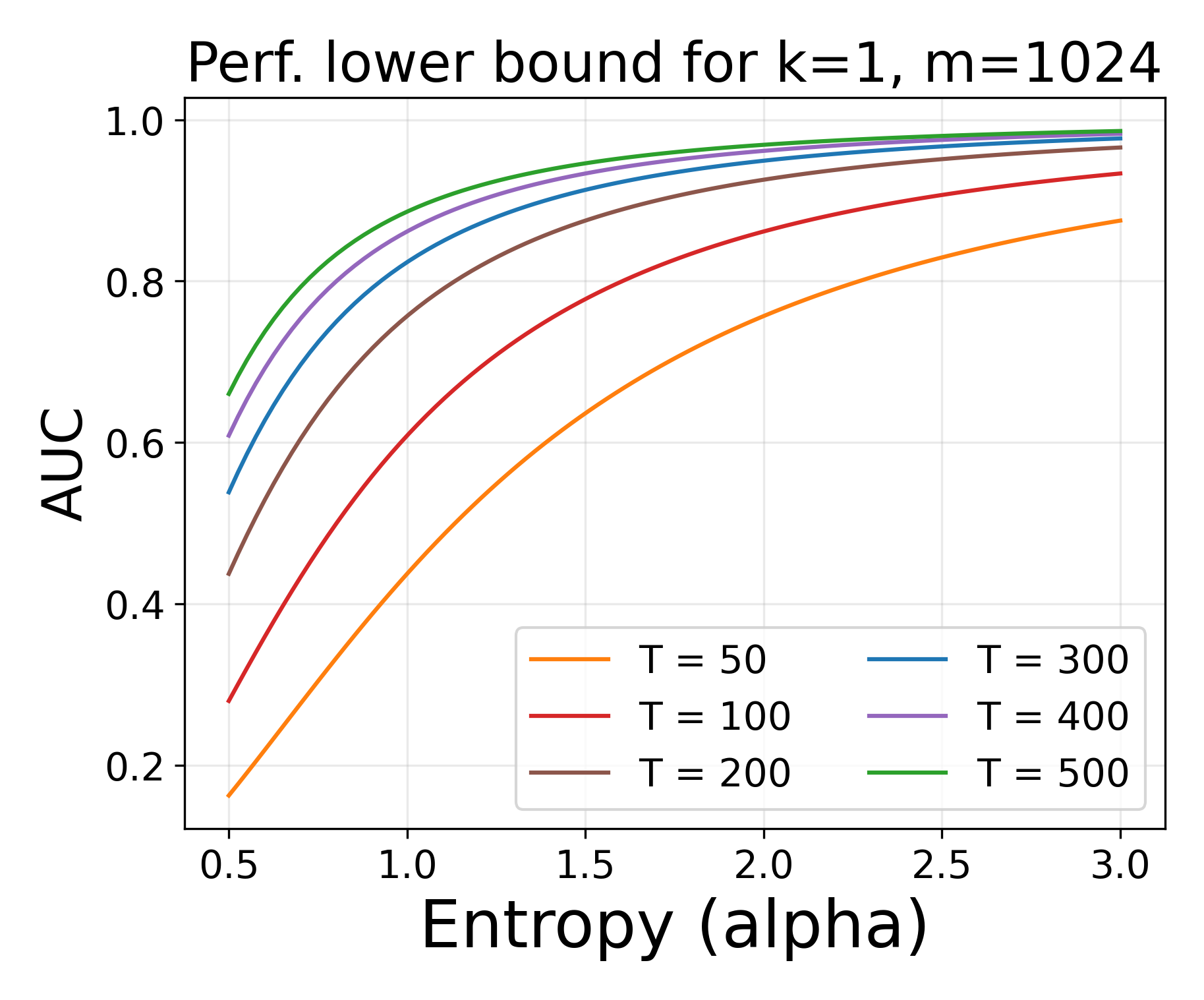
Theorem 4.2 connects detection performance to the language model’s underlying distribution, number of sampled tokens , and number of test samples . More entropy and more test samples guarantee higher performance. When the model is extremely confident, and so does our lower bound. Note that because measures the entropy of the empirical distribution arising from sampling tokens, it depends on both the underlying next-token probability distribution as well as . Concretely, when conditioned on the next-token probabilities , . The largest is achieved when the nonzero ’s are 1, which can occur when the underlying distribution is uniform (maximal uncertainty) and/or is not large. In this case, and our bound goes to . This quantity has very sharp diminishing returns with respect to , so there may be little value in increasing beyond a certain point. When , the bound goes to , which increases very quickly with . A mere 50 test tokens guarantees at least ROC-AUC. We study the interplay of the various factors on our lower bound more carefully in the Appendix.
The intuitions here carry over to other choices of and , though formal bounds can be tricky to obtain because of difficulty quantifying the alternative distribution. The null distribution is easy — -values are under , and as a result, we have a straightforward equality on the false positive rate.
Theorem 4.3 (False positive rate).
No matter the choice of watermarking settings, assuming that the unique test -grams are independent, we have the following equality on the false positive rate of Detect, using decision threshold .
This also holds for DetectRecursive if we further assume the -values across secret keys are independent.
Selecting distinct independent secret keys (and ignoring hash collisions that arise across calls to Detect within DetectRecursive), will help attain the necessary independence.
Although the alternative score distribution is generally intractable, with the strong assumption that there are no duplicate -grams across the candidate sequences, then for a special choice of , we can write the alternative in closed form and formulate the optimal detection test.
Theorem 4.4 (Optimal detection for Gamma).
Assume that candidate sequences are unique with length and that the -grams are independent and contain no duplicates. Suppose we choose (flat scheme), for any rate parameter . Let with pdf , with pdf , and the PRF values of the test tokens (unique -grams), assumed to be independent. Then, , under the null that the text was watermarked using our procedure and otherwise. The uniformly most powerful test is the log-likelihood ratio test (LRT) with score
Furthermore, for any decision threshold on score , we have that:
| FPR (Type-I error) | |||
| FNR (Type-II error) | |||
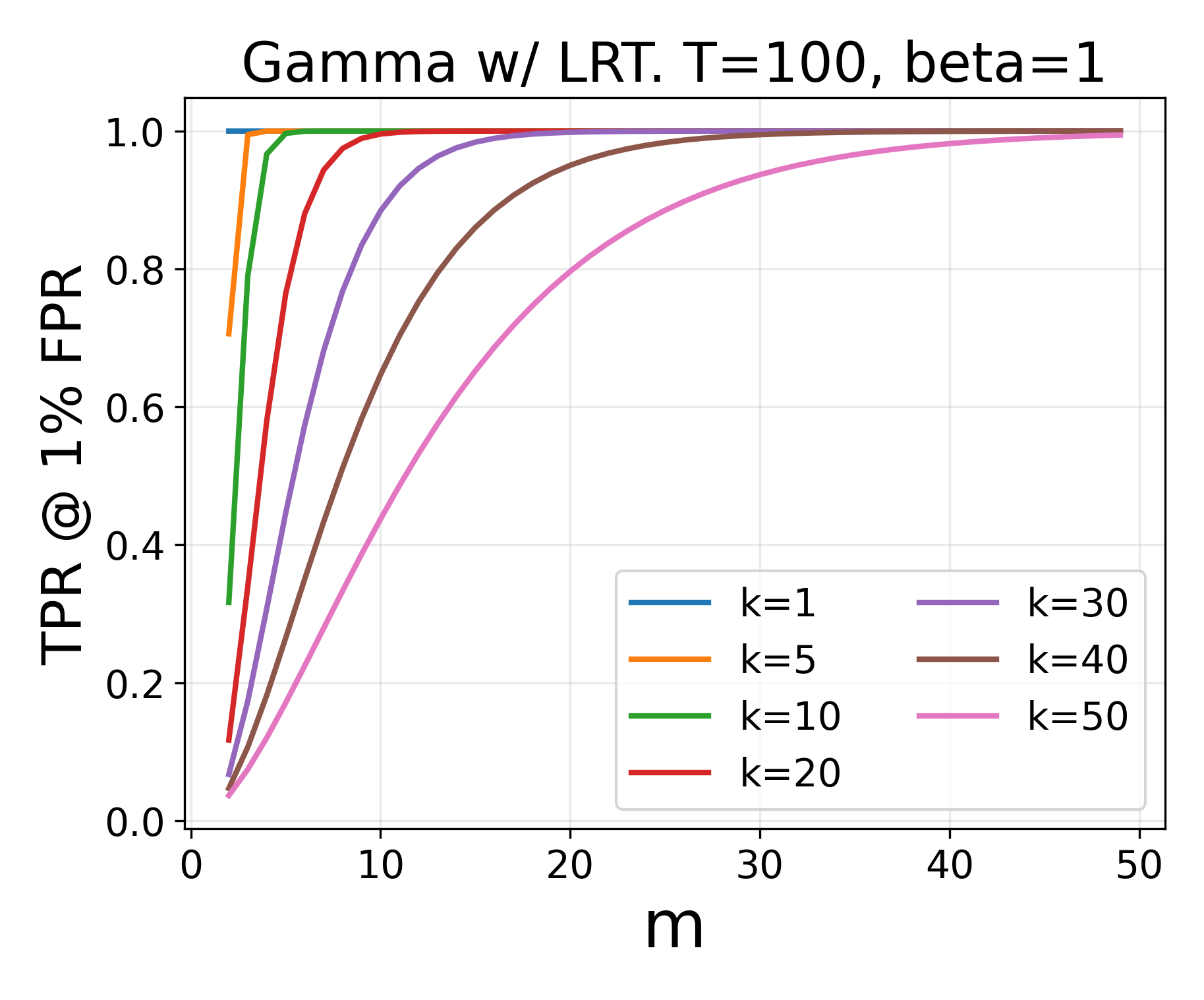
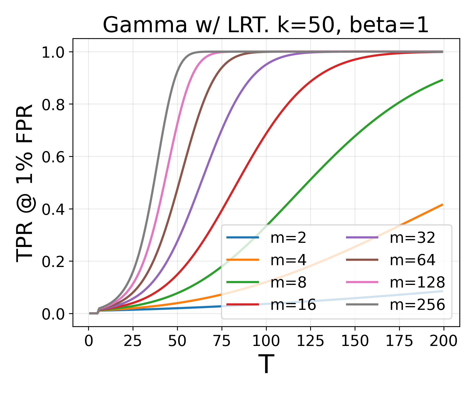
In the Appendix, we use Theorem 4.4 to study the impact of , , and on TPR at fixed FPR. For example, with , , , , we can achieve TPR at FPR.
For other choices of , we can estimate via simulation. If we assume candidate sequences have the same length with no duplicate -grams, then we can fill an matrix with i.i.d. draws from and pick the first element of the row with the largest row-sum (among the ). We do this until we have sufficiently large (e.g. 10,000) samples from . We apply a Gaussian kernel-density estimator where the bandwidth is chosen using Scott’s rule (Scott, 2015) to estimate for test value . Despite having in closed-form, for consistency, we can also estimate it non-parametrically by drawing from .
5 Experiments
In this section, we compare the performance of our scheme with that of prior work.
5.1 Models, Datasets, and Hyperparameters
Models and Datasets. Our main model and dataset is Mistral-7B-instruct (Jiang et al., 2023) hosted on Huggingface222https://huggingface.co/mistralai/Mistral-7B-Instruct-v0.1 with bfloat16 quantization, and databricks-dolly-15k333https://huggingface.co/datasets/databricks/databricks-dolly-15k (Conover et al., 2023), an open source dataset of instruction-following examples for brainstorming, classification, closed QA, generation, information extraction, open QA, and summarization. We use prompts from the brainstorming, generation, open QA (i.e. general QA), and summarization categories, whose human responses are at least 50 tokens long (save one example, which was removed because the prompt was extremely long). For each of the 5233 total prompts, we generate two non-watermarked responses — a stochastic one using temperature 1, and the greedy / argmax decoding — along with a watermarked one for each scheme. We always force a minimum (maximum) of 250 (300) new tokens by disabling the stop token for the first 250 tokens, re-enabling it, and stopping the generation at 300, regardless of whether the stop token was encountered. To simulate real-world use, we de-tokenize the outputs to obtain plain text, and re-tokenize them during scoring. We study performance as a function of token length by truncating to the first tokens.
For completeness, we also present the key results when Gemma-7B-instruct444https://huggingface.co/google/gemma-7b-it with bfloat16 quantization is applied to the test split of eli5-category555https://huggingface.co/datasets/rexarski/eli5_category. Prompts are formed by concatenating the the title and selftitle fields. Only examples with non-empty title and whose prompt contains a ? are kept — for a total of 4885 examples.
Hyperparameters. We consider the following choices of CDFs / . (1) and . (2) and . (3) and . (4) and .
5.2 Evaluation Metrics
We evaluate performance using three criteria.
Detectability. How well can we discriminate between non-watermarked and watermarked text? We choose non-watermarked text to be text generated by the same model, just without watermarking applied during decoding. There are three reasons for choosing the negative class in this way. Firstly, it makes controlling for text length easier as we can generate as many tokens as we do for watermarked samples — in contrast, human responses are of varying lengths. Secondly, watermarked text has far more token / -gram overlap with its non-watermarked counterpart than the human reference, which makes detection more challenging. Lastly, since one intended use case of our scheme is for third-party users of a shared LLM service, users may want to distinguish between their watermarked text and non-watermarked text generated by the same LLM service.
Our primary one-number metric is ROC-AUC for this balanced binary classification task. Since performance at low FPR is often more useful in practice, we report the partial ROC-AUC (pAUC) for FPR a target FPR (taken to be 1%), which we find to be more meaningful than TPR at the target FPR. We look at performance as a function of length by truncating the positive and negatives samples to lengths . To understand aggregate performance, we pool all different length samples together and compute one ROC-AUC. Here, it is paramount that the detection score be length-aware to ensure that a single decision threshold can be used across lengths.
Distortion. Our scheme, along with most of the baselines, boasts a distortion-free property. This property comes with assumptions that are often violated in practice, for example by reuse of the secret key across watermarking calls. We quantify how faithful the watermarking procedure is to the underlying generative model by computing both the perplexity and likelihood of watermarked text under the generator (without watermarking). We include likelihood as the log-probabilities used in calculating perplexity can over-emphasize outliers.
Quality. Watermarking may distort the text per the model, but does the distortion tangibly affect the quality of the text? Quality can be challenging to define and measure — one proxy is likelihood under a much larger model than the generator. Alternatively, one can run standard benchmark NLP tasks and use classic metrics like exact match, etc. We instead opt for using Gemini-1.5-Pro as an LLM judge and compute pairwise win rates for each watermark strategy against no watermarking (greedy decoding). We do this in two ways for each scheme — (1) we compute win rates using a single response for each prompt and (2) we first ask the LLM judge to pick the best of 3 responses for each prompt and compute win rates using the best response. (2) represents the common practice of sampling a few generations from the LLM and selecting the best one using some criterion. It captures diversity, as methods that can express an answer in a few different good ways will have an advantage. A caveat with win rates is that they may not reflect the degree by which one method is better or worse. For instance, if one strategy’s output was always marginally worse than no watermarking, the win rate would be 0% — the same as if it were much worse.
5.3 Adversarial Attacks
An adversary in possession of watermarked text (but who lacks knowledge of the secret key) may try to evade detection. We study how detectability degrades under two attack strategies —- random token replacement and paraphrasing.
Random token replacement. Here, we take the watermarked tokens and a random -percent of them are corrupted by replacing each with a random different token. is taken to be . This attack strategy is cheap for the adversary to carry out but will significantly degrade the quality of the text.
Paraphrasing. In this attack, the adversary attempts to evade detection by paraphrasing the watermarked text. We use Gemini-1.5-Pro to paraphrase each non-truncated watermarked generation. Details are deferred to the Appendix.
| PPL | WR | WR (3) | AUC | pAUC | C. AUC | C. pAUC | P. AUC | P. pAUC | |
| Max Std. Error | 0.03 | - | - | 0.1 | 0.3 | 0.2 | 0.3 | - | - |
| Greedy Decoding | 1.37 | - | - | - | - | - | - | - | - |
| Random Sampling | 3.50 | 49.6 | 65.3 | - | - | - | - | - | - |
| Aaronson | 2.81 | 45.3 | 45.3 | 71.7 | 65.5 | 65.6 | 60.3 | 53.9 | 50.5 |
| Aaronson Cor. | 2.81 | 45.3 | 45.3 | 97.9 | 83.6 | 94.8 | 73.2 | 58.8 | 50.7 |
| Kuditipudi | 3.55 | 50.3 | 67.3 | 87.8 | 76.6 | 87.2 | 74.4 | 75.9 | 53.2 |
| Kirchenbauer | 3.39 | 49.6 | 66.6 | 73.2 | 52.0 | 71.0 | 51.4 | 49.0 | 49.8 |
| 3.37 | 50.1 | 67.0 | 86.9 | 60.6 | 83.7 | 57.1 | 52.9 | 49.9 | |
| 3.69 | 47.9 | 64.1 | 97.0 | 83.3 | 95.4 | 77.4 | 58.4 | 50.3 | |
| 4.67 | 41.5 | 58.4 | 99.3 | 94.4 | 98.6 | 90.9 | 63.4 | 51.5 | |
| 5.81 | 26.0 | 41.2 | 99.8 | 98.4 | 99.6 | 96.8 | 66.4 | 52.7 | |
| Flat | 3.46 | 50.0 | 66.4 | 90.2 | 68.8 | 82.0 | 58.7 | 50.5 | 50.3 |
| 3.36 | 50.8 | 67.0 | 95.8 | 82.9 | 90.3 | 70.5 | 51.3 | 50.6 | |
| 3.20 | 47.7 | 64.5 | 97.7 | 89.7 | 93.9 | 79.1 | 52.7 | 51.1 | |
| 3.06 | 48.4 | 65.3 | 97.8 | 90.2 | 94.2 | 80.0 | 53.0 | 50.8 | |
| 2.63 | 47.7 | 62.5 | 97.7 | 90.0 | 94.1 | 79.7 | 54.6 | 51.3 | |
| 2.61 | 47.7 | 62.2 | 97.7 | 90.0 | 94.0 | 79.7 | 52.8 | 51.1 | |
| Flat | 4.10 | 46.1 | 62.2 | 83.4 | 55.8 | 73.6 | 52.0 | 49.0 | 50.0 |
| 4.06 | 45.2 | 61.5 | 93.8 | 72.7 | 85.7 | 59.4 | 51.3 | 50.3 | |
| 3.86 | 44.6 | 60.6 | 97.8 | 87.0 | 93.1 | 73.5 | 54.3 | 50.7 | |
| 3.80 | 43.0 | 60.8 | 98.2 | 89.0 | 94.0 | 76.7 | 55.0 | 50.8 | |
| Flat | 3.79 | 48.5 | 64.2 | 69.6 | 50.7 | 62.2 | 50.3 | 47.0 | 50.0 |
| 3.76 | 47.7 | 63.9 | 82.9 | 53.5 | 71.9 | 51.3 | 49.4 | 50.0 | |
| 3.72 | 48.3 | 64.2 | 92.7 | 66.7 | 83.1 | 55.6 | 50.5 | 50.1 | |
| 3.67 | 47.3 | 63.9 | 94.2 | 71.6 | 85.5 | 58.1 | 51.1 | 50.5 | |
| Rec. | 3.41 | 49.0 | 65.0 | 93.4 | 75.5 | 86.3 | 63.2 | 48.4 | 50.4 |
| 3.33 | 49.2 | 66.2 | 95.4 | 82.9 | 90.6 | 71.8 | 53.4 | 50.8 | |
| 3.29 | 48.4 | 64.3 | 96.3 | 85.0 | 91.6 | 73.5 | 49.4 | 50.8 | |
| 3.05 | 48.3 | 64.5 | 97.2 | 87.9 | 92.6 | 76.5 | 50.4 | 51.2 | |
| Rec. | 4.13 | 45.7 | 61.3 | 88.6 | 61.7 | 78.8 | 53.8 | 48.0 | 50.0 |
| 4.13 | 43.7 | 59.7 | 93.4 | 74.0 | 86.8 | 61.6 | 52.9 | 50.4 | |
| 4.06 | 42.9 | 59.5 | 94.8 | 76.9 | 88.1 | 63.2 | 50.6 | 50.3 | |
| Rec. | 3.79 | 48.2 | 63.8 | 74.2 | 51.2 | 65.1 | 50.5 | 46.5 | 49.9 |
| 3.77 | 47.0 | 64.0 | 81.2 | 54.5 | 73.3 | 51.9 | 51.4 | 50.2 | |
| 3.79 | 47.2 | 63.3 | 83.3 | 55.7 | 74.4 | 52.2 | 49.4 | 50.0 |
5.4 Baselines
The watermark schemes we consider here operate token-by-token in the autoregressive decoding loop. Let be the next-token probability distribution. Higher detection scores indicate higher confidence that the query text is watermarked.
Aaronson (A). Aaronson (2023) computes a PRN for each token in the vocabulary as , where is the preceding -gram, is the secret key and is a cryptographic hash. Token is selected, where . At test time, -grams are extracted from the query test and the detection score is , where . is set to 4. This choice strikes a good balance between generation quality / diversity and robustness to attacks. The scheme boasts a distortion-free property, but the generated text is a deterministic function of the prompt — i.e. only one generation is possible conditioned on a particular prompt.
Remark.
If and , then our watermark encoding can be viewed as a stochastic version of Aaronson (2023)’s. As , , where and are the probability and observed occurrences of token .
Aaronson Corrected (AC). Aaronson (2023)’s detection score is not length-aware and consequently a single decision threshold across scores involving various lengths results in poor performance, as we later show. Observing that is a sum of log -values, , or equivalently, under the null that all test tokens are non-watermarked. We propose the new corrected detection score, . For completeness we also experiment with a -value computed in the way we do for our method — concretely as, . Note that both transformations are monotonic so they have no effect on ROC-AUC when T is fixed.
Kirchenbauer (KB). Kirchenbauer et al. (2023a) uses the previous tokens to pseudorandomly partition the vocabulary for the next token into two lists: a green list of size and a red list consisting of the remainder. A positive bias of is added to the logits of the green list tokens while those of the red list are left unchanged. This has the effect of modifying so that green list tokens are more probable. The score for a text consisting of tokens, of which were found to be green is, . We incorporate the latest updates to the algorithm,666https://github.com/jwkirchenbauer/lm-watermarking such as including the current token in the -gram and skipping duplicate -grams at test time. We set , , and .
Kuditipudi (K). A drawback of using the last tokens as a basis for the PRF is that changing just one of them changes the output and hurts detection. Kuditipudi et al. (2023) addresses this limitation as follows. Consider a secret, finite ordered list of seeds of length . Start watermarking by selecting a position in the seed list uniformly at random and apply the selection rule of Aaronson (2023) with the PRNG seeded to the current value. Advance to the next seed in the list (wrap-around if you are at the end) and repeat. Scoring is done by conducting a permutation test evaluating how compatible the query text is with the specific list of seeds used during encoding as opposed to any other random list of seeds of the same length. As the random starting position is not known during scoring, an alignment score based on the Levenshtein distance is given that considers alignments of various subsequences of the text and seeds. The proposed method is quite similar to Aaronson (2023) with the difference of using a fixed list of seeds (instead of input tokens to determine the seed) and using a permutation test for scoring. The upside is robustness to token substitution attacks; the downside is significantly higher computational cost for scoring. Larger offers more diversity and quality in generation but comes with costlier and weaker detection. The scheme is distortion-free. Following their work, we let and accelerate the permutation test by pre-computing 5000 reference values for the secret list using snippets from the train set of C4-realnewslike (Raffel et al., 2019) at the various target lengths we evaluate on.
5.5 Experimental Results
Table 1 shows results for baselines and our scheme using and -values for scoring, as detailed in Algorithms 1 and 2. For the recursive scheme, depth is (i.e. for each imaginary watermarker). Here, the negative class is non-watermarked argmax/greedy generations. Results for using stochastic (temperature 1) generations as the negative as well as the average likelihood scores are presented in Table 5 (Appendix); the trends remain the same. We summarize our observations on Mistral-7B-instruct on databricks-dolly-15k, which also hold for Gemma-7B-instruct on eli5-category (presented in the Appendix).
5.5.1 Overall performance of our flat and recursive schemes
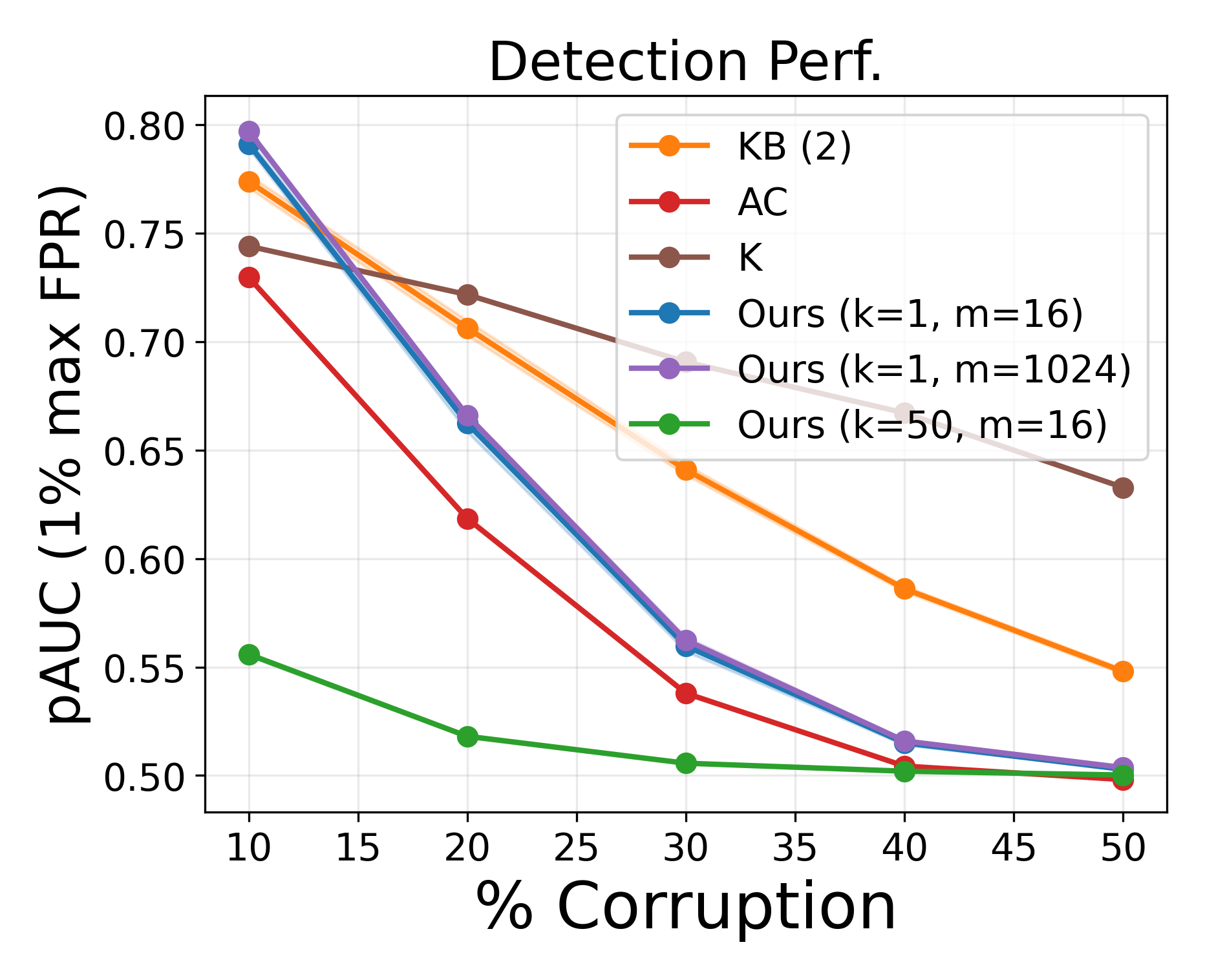
Our scheme is a competitive option for white-box watermarking. Is it better to use our method or alternatives in the white-box setting? When , we are able to achieve better perplexity (2.61 vs. 2.81), better diversity (62.2% vs. 45.3% on best-of-3 win rates) and comparable detection performance than Aaronson (2023). Furthermore, it has better perplexity (2.61 vs. 3.55) and detection performance (97.7% vs. 87.8% AUC) than Kuditipudi et al. (2023). By cranking up , Kirchenbauer et al. (2023a) can achieve strong detection but at the expense of perplexity. When matched on perplexity, we achieve better detection. For example, achieves 3.39 PPL and 73.2% AUC compared to our 2.61 PPL and 97.7% AUC. Gemma-7B-instruct on eli5-category with outperforms Kuditipudi et al. (2023) and is on-par with Aaronson (2023) (see Appendix). Kirchenbauer et al. (2023a) with gives 1.649 PPL and 61.6% AUC whereas gets us 1.610 PPL with 93.2% AUC and even 1.645 PPL with 89.7% AUC when (black-box).
Flat watermarking outperforms recursive. Across metrics and settings we see that the flat scheme outperforms its recursive counterpart, suggesting it is more effective when a strong signal is embedded using a single key rather than when multiple weak signals are embedded with different keys. For example, when flat (recursive) PPL and AUC are 3.06 (3.29) and 97.8% (96.3%) respectively.
5.5.2 Effects of Hyperparameters
Increasing improves perplexity but hurts diversity. Across ’s, we observe that perplexity decreases as increases, but that win rates, especially when best-of-3 generations are used, decrease. For example, when , increasing from 2 to 1024 decreases perplexity from 3.46 to 2.61 but also drops the best-of-3 win rate from 66.4% to 62.2%. As remarked earlier, as , and our scheme becomes less diverse — deterministic conditioned on the prompt, like Aaronson’s. On the flip side, large reduces sampling noise which drives down perplexity.
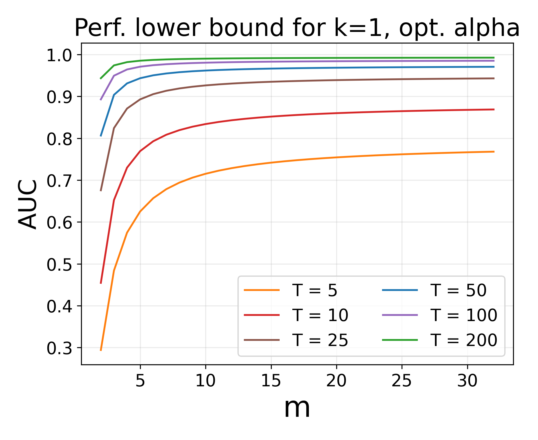
Increasing improves detection but has diminishing returns. Across the board we see that detection improves as increases, but there are diminishing returns. For example, when , our AUC increases from 90.2% to 95.8% as goes from 2 to 4, but flattens out when hits 16. This corroborates our theoretical intuition from Theorem 4.2 which is further explored in Figure 4 (Appendix).
For fixed , increasing hurts detection performance. For fixed and target generation length , increasing gives us fewer opportunities (fewer calls to WatermarkSingle) to inject the watermark signal, and detection consequently suffers. For example, when , AUC drops from 97.8% to 94.2% when increases from 1 to 50.
slightly outperforms alternative distributions. Flat distributions may offer better robustness to attacks. In Table 4 (Appendix), we see that fares comparably to and slightly outperforms both on detection and perplexity. For example, when , and have AUCs of 69.6% and 68.1% respectively. Furthermore, we find evidence that offers better protection to attacks. For example, when , the AUC for ( degrades from 94.2% (94.5%) to 85.5% (84.5%) in the presence of 10% random token corruption. We provide some intuition for why flat distributions like may be more robust than those with quickly decaying tails. Consider shaping the continuous so it approaches (i.e. ), where is very small. Suppose is large and is small. Then, the winning sequence will have extremely few (if any) of its ’s equal to . If the text is unmodified and these few -grams are kept intact, we are fine, but if they are corrupted in an attack, then the watermarking signal is effectively lost. In other words, flat distributions smear the watermarking signal over more tokens than do sharper distributions, which localize the signal to few lucky token positions. However, whereas scoring with when involves computing -fold convolutions or cardinal B-splines, when , is easier to compute for very large ; specifically, .
5.5.3 Observations on detection
Length correction of Aaronson (2023) is crucial. Recall that the ROC-AUCs presented in Table 1 are computed over a pool of different lengths. Our -value-based score for Aaronson (2023) improves detection significantly; for example, AUC goes from 71.7% to 97.9%. Table 7 (Appendix) shows that the sum-based -value correction fares a bit worse, which was a little surprisingly given that this worked the best for our scheme, even for the case.
Sum-based -values outperform Fisher ones. In Table 2 (Appendix), we observe that replacing our sum-based -value (where is that ) by a Fisher combination of token-level -values hurts detection performance. For example, when , AUC degrades from 90.2% to 86.3%. Note that when , this setting corresponds exactly to a stochastic version of Aaronson (2023).
Likelihood-ratio scoring does well for large and small , when its assumptions are more realistic. In Table 3 (Appendix), we observe that likelihood-based scoring — both when the distribution is Gamma and the exact likelihood ratio test (LRT) is used and under KDE with alternative distributions — performs the best when the assumptions of no duplicate sequences or -grams hold better. This happens when the sequences are long (large ) and when fewer sequences are sampled (small ). For example, when , AUC degrades monotonically from 78.1% to 55.4% as increases from to . In contrast, AUC under the -value-based scoring increases monotonically with , from 90.2% to 97.7%. Larger increases the number of duplicate sequences sampled, increasing the importance of the latent exponent used in the scoring and deviating us further from the LRT assumptions. However, LRT has the potential to be an effective alternative when is large. For example, when and , Uniform KDE-based LRT gives AUC of 95.5% compared to -value’s 94.2%.
Detection performance improves sharply with test samples . Figure 1 shows the effect of on AUC. We see sharp improvements w.r.t. to , even when is large and is small, highlighting the power of more test samples to counteract a weaker watermark signal.
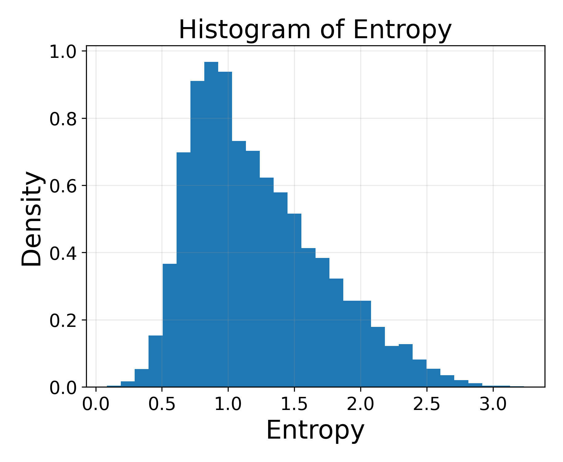
Entropy improves detection performance. In Figure 1 we bucket prompts based on the entropy of their non-watermarked response and then look at detection AUC on samples in each bucket. As we expect, detection improves when the prompts confer more entropy in the response. This trend is more stark for our method.
Paraphrasing can be extremely effective at destroying watermarks. We observe that paraphrasing can effectively erase the watermark as detection performance for most methods is near random. Kuditipudi et al. (2023) and Kirchenbauer et al. (2023a) with large do better on AUC (but not so much on pAUC). Furthermore, in Figures 1 and 2 (Appendix) we observe that large amounts of random token corruption hurts our scheme and Aaronson (2023)’s more than it that of Kirchenbauer et al. (2023a) or Kuditipudi et al. (2023).
6 Conclusion
In this work, we present a framework for watermarking language models that requires nothing more than a way to sample from them. Our framework is general and extensible, supporting various real world use-cases, including the setting where the next-token probabilities are in fact available. We study its various components and the trade-offs that arise, provide formal guarantees for the theoretically-inclined as well as concrete recommendations for the practitioner.
Acknowledgements
The authors would like to thank Rob McAdam, Abhi Shelat, Matteo Frigo, Ashkan Soleymani, John Kirchenbauer, and Mukund Sundararajan for insightful discussions without which this work would not be possible.
References
- Aaronson (2023) Scott Aaronson. Watermarking of large language models. Large Language Models and Transformers Workshop at Simons Institute for the Theory of Computing, 2023.
- Carlini et al. (2024) Nicholas Carlini, Daniel Paleka, Krishnamurthy Dj Dvijotham, Thomas Steinke, Jonathan Hayase, A Feder Cooper, Katherine Lee, Matthew Jagielski, Milad Nasr, Arthur Conmy, et al. Stealing part of a production language model. arXiv preprint arXiv:2403.06634, 2024.
- Chang et al. (2024) Yapei Chang, Kalpesh Krishna, Amir Houmansadr, John Wieting, and Mohit Iyyer. Postmark: A robust blackbox watermark for large language models. arXiv preprint arXiv:2406.14517, 2024.
- Christ & Gunn (2024) Miranda Christ and Sam Gunn. Pseudorandom error-correcting codes. arXiv preprint arXiv:2402.09370, 2024.
- Christ et al. (2023) Miranda Christ, Sam Gunn, and Or Zamir. Undetectable watermarks for language models. arXiv preprint arXiv:2306.09194, 2023.
- Conover et al. (2023) Mike Conover, Matt Hayes, Ankit Mathur, Jianwei Xie, Jun Wan, Sam Shah, Ali Ghodsi, Patrick Wendell, Matei Zaharia, and Reynold Xin. Free dolly: Introducing the world’s first truly open instruction-tuned llm, 2023. URL https://www.databricks.com/blog/2023/04/12/dolly-first-open-commercially-viable-instruction-tuned-llm.
- Devlin (2018) Jacob Devlin. Bert: Pre-training of deep bidirectional transformers for language understanding. arXiv preprint arXiv:1810.04805, 2018.
- Fernandez et al. (2023) Pierre Fernandez, Antoine Chaffin, Karim Tit, Vivien Chappelier, and Teddy Furon. Three bricks to consolidate watermarks for large language models. In 2023 IEEE International Workshop on Information Forensics and Security (WIFS), pp. 1–6. IEEE, 2023.
- Gu et al. (2023) Chenchen Gu, Xiang Lisa Li, Percy Liang, and Tatsunori Hashimoto. On the learnability of watermarks for language models. arXiv preprint arXiv:2312.04469, 2023.
- Hou et al. (2023) Abe Bohan Hou, Jingyu Zhang, Tianxing He, Yichen Wang, Yung-Sung Chuang, Hongwei Wang, Lingfeng Shen, Benjamin Van Durme, Daniel Khashabi, and Yulia Tsvetkov. Semstamp: A semantic watermark with paraphrastic robustness for text generation. arXiv preprint arXiv:2310.03991, 2023.
- Huang et al. (2023) Baihe Huang, Banghua Zhu, Hanlin Zhu, Jason D Lee, Jiantao Jiao, and Michael I Jordan. Towards optimal statistical watermarking. arXiv preprint arXiv:2312.07930, 2023.
- Jiang et al. (2023) Albert Q Jiang, Alexandre Sablayrolles, Arthur Mensch, Chris Bamford, Devendra Singh Chaplot, Diego de las Casas, Florian Bressand, Gianna Lengyel, Guillaume Lample, Lucile Saulnier, et al. Mistral 7b. arXiv preprint arXiv:2310.06825, 2023.
- Kirchenbauer et al. (2023a) John Kirchenbauer, Jonas Geiping, Yuxin Wen, Jonathan Katz, Ian Miers, and Tom Goldstein. A watermark for large language models. arXiv preprint arXiv:2301.10226, 2023a.
- Kirchenbauer et al. (2023b) John Kirchenbauer, Jonas Geiping, Yuxin Wen, Manli Shu, Khalid Saifullah, Kezhi Kong, Kasun Fernando, Aniruddha Saha, Micah Goldblum, and Tom Goldstein. On the reliability of watermarks for large language models. arXiv preprint arXiv:2306.04634, 2023b.
- Krishna et al. (2024) Kalpesh Krishna, Yixiao Song, Marzena Karpinska, John Wieting, and Mohit Iyyer. Paraphrasing evades detectors of ai-generated text, but retrieval is an effective defense. Advances in Neural Information Processing Systems, 36, 2024.
- Kuditipudi et al. (2023) Rohith Kuditipudi, John Thickstun, Tatsunori Hashimoto, and Percy Liang. Robust distortion-free watermarks for language models. arXiv preprint arXiv:2307.15593, 2023.
- Lee et al. (2023) Taehyun Lee, Seokhee Hong, Jaewoo Ahn, Ilgee Hong, Hwaran Lee, Sangdoo Yun, Jamin Shin, and Gunhee Kim. Who wrote this code? watermarking for code generation. arXiv preprint arXiv:2305.15060, 2023.
- Liu et al. (2023a) Aiwei Liu, Leyi Pan, Xuming Hu, Shu’ang Li, Lijie Wen, Irwin King, and Philip S Yu. An unforgeable publicly verifiable watermark for large language models. arXiv preprint arXiv:2307.16230, 2023a.
- Liu et al. (2023b) Aiwei Liu, Leyi Pan, Xuming Hu, Shiao Meng, and Lijie Wen. A semantic invariant robust watermark for large language models. arXiv preprint arXiv:2310.06356, 2023b.
- Raffel et al. (2019) Colin Raffel, Noam Shazeer, Adam Roberts, Katherine Lee, Sharan Narang, Michael Matena, Yanqi Zhou, Wei Li, and Peter J. Liu. Exploring the limits of transfer learning with a unified text-to-text transformer. arXiv e-prints, 2019.
- Ren et al. (2023) Jie Ren, Han Xu, Yiding Liu, Yingqian Cui, Shuaiqiang Wang, Dawei Yin, and Jiliang Tang. A robust semantics-based watermark for large language model against paraphrasing. arXiv preprint arXiv:2311.08721, 2023.
- Scott (2015) David W Scott. Multivariate density estimation: theory, practice, and visualization. John Wiley & Sons, 2015.
- Thibaud et al. (2024) Gloaguen Thibaud, Jovanović Nikola, Staab Robin, and Vechev Martin. Black-box detection of language model watermarks. arXiv preprint arXiv:2405.20777, 2024.
- Venugopal et al. (2011) Ashish Venugopal, Jakob Uszkoreit, David Talbot, Franz Josef Och, and Juri Ganitkevitch. Watermarking the outputs of structured prediction with an application in statistical machine translation. In Proceedings of the 2011 Conference on Empirical Methods in Natural Language Processing, pp. 1363–1372, 2011.
- Yang et al. (2023) Xi Yang, Kejiang Chen, Weiming Zhang, Chang Liu, Yuang Qi, Jie Zhang, Han Fang, and Nenghai Yu. Watermarking text generated by black-box language models. arXiv preprint arXiv:2305.08883, 2023.
- Yoo et al. (2023) KiYoon Yoo, Wonhyuk Ahn, Jiho Jang, and Nojun Kwak. Robust multi-bit natural language watermarking through invariant features. In Proceedings of the 61st Annual Meeting of the Association for Computational Linguistics (Volume 1: Long Papers), pp. 2092–2115, 2023.
- Zhang et al. (2023) Hanlin Zhang, Benjamin L Edelman, Danilo Francati, Daniele Venturi, Giuseppe Ateniese, and Boaz Barak. Watermarks in the sand: Impossibility of strong watermarking for generative models. arXiv preprint arXiv:2311.04378, 2023.
- Zhao et al. (2023) Xuandong Zhao, Prabhanjan Ananth, Lei Li, and Yu-Xiang Wang. Provable robust watermarking for ai-generated text. arXiv preprint arXiv:2306.17439, 2023.
Appendix A Appendix
A.1 Additional Experimental Details
Prompting strategies for Gemini. We use Gemini for paraphrasing and as an LLM judge. Occasionally, Gemini will refuse to return a response due to safety filters that cannot be bypassed. We use the following prompt to compute win rates:
“Is (A) or (B) a better response to PROMPT? Answer with either (A) or (B). (A): GREEDY RESPONSE. (B): WATERMARKED RESPONSE.”
For determining the best response, we use:
“Is (A), (B), or (C) the best responses to PROMPT? Answer with either (A), (B), (C). (A): RESPONSE 1. (B): RESPONSE 2. (C): RESPONSE 3.”
In both cases, we search for the first identifier (i.e. “(A)”, “(B)”, “(C)”). If one is not found or if Gemini does not return a response, the example is not used in the win rate calculation or the first response is chosen.
For paraphrasing, we use the following:
“Paraphrase the following: RESPONSE”.
We skip examples for which Gemini does not return a response.
A.2 Omitted Experimental Results
Figure 2 shows the effect of varying the amount of random token corruption on detection pAUC. We observe the same trend as for AUC. Figure 3 plots a histogram of the entropy of the underlying next-token probability distribution under temperature 1 random sampling without watermarking across our dataset. We see the entropy is concentrated between 0.5 and 3 nats. We plot the AUC lower bound predicted by Theorem 4.2 () sweeping our entropy term across this range, with the understanding that for sufficiently large , our is a good estimator of the true underlying entropy. In Figure 4 we look at the impact of and on our AUC bound when the optimal is plugged in. We see sharp diminishing returns w.r.t. (performance saturates after around for all ’s). We empirically observe this saturation in Table 1, where AUC saturates at 97.7% at — that is, increasing beyond 16 has negligible impact. Furthermore, we observe that the bound increases sharply with , corroborating the trend we see empirically in Figure 1.
Given a next-token distribution over the vocabulary, we can estimate via simulation. In Figure 5 we plot the effect of on , our simulated entropy, for two distributions — uniform and Zipf — over a 32k token vocabulary. Neither may be realistic in practice, but the exercise is still informative as we observe that follows pretty well for even large ’s when is uniform. As expected, is smaller when is Zipf (lower entropy) and deviates from for large .
Figure 7 plots the performance that Theorem 4.4 predicts when using the optimal likelihood ratio test with the Gamma distribution.
Table 6 shows perplexity and detection performance for Gemma-7B-instruct on the eli5-category dataset. The trends here are as before. Figure 6 shows the impact of number of test samples on detection.
| PPL | LH | AUC | pAUC | C. AUC | C. pAUC | |
| Max Std. Error | 0.03 | 0.002 | 0.1 | 0.1 | 0.2 | 0.1 |
| Unif. Fisher -value | ||||||
| Flat | 3.46 | 0.597 | 86.3 | 62.3 | 75.8 | 54.7 |
| 3.36 | 0.604 | 94.8 | 79.0 | 87.6 | 66.4 | |
| 3.20 | 0.618 | 97.9 | 90.0 | 94.0 | 80.2 | |
| 3.06 | 0.629 | 98.2 | 91.7 | 94.9 | 82.7 | |
| 2.63 | 0.668 | 98.5 | 93.0 | 95.7 | 85.5 | |
| 2.61 | 0.670 | 98.5 | 93.2 | 95.7 | 85.8 | |
| Flat | 4.10 | 0.568 | 78.9 | 53.1 | 67.4 | 51.0 |
| 4.06 | 0.572 | 91.2 | 65.3 | 80.5 | 55.0 | |
| 3.86 | 0.583 | 97.1 | 82.8 | 90.9 | 68.1 | |
| 3.80 | 0.587 | 97.9 | 86.3 | 92.7 | 72.7 | |
| Flat | 3.79 | 0.581 | 65.5 | 50.5 | 57.1 | 50.2 |
| 3.76 | 0.584 | 78.4 | 52.0 | 66.1 | 50.7 | |
| 3.72 | 0.586 | 89.8 | 60.2 | 77.9 | 53.1 | |
| 3.67 | 0.589 | 92.0 | 64.7 | 80.7 | 54.5 |
| PPL | LH | AUC | pAUC | C. AUC | C. pAUC | |
| Max Std. Error | 0.03 | 0.002 | 0.1 | 0.3 | 0.2 | 0.1 |
| Unif. KDE LRT | ||||||
| Flat | 3.46 | 0.597 | 78.1 | 57.7 | 64.4 | 51.5 |
| 3.36 | 0.604 | 73.9 | 56.0 | 60.7 | 51.2 | |
| 3.20 | 0.618 | 66.6 | 53.9 | 56.7 | 51.3 | |
| 3.06 | 0.629 | 64.0 | 53.6 | 55.2 | 51.3 | |
| 2.63 | 0.668 | 56.2 | 51.3 | 50.4 | 50.3 | |
| 2.61 | 0.670 | 55.4 | 51.1 | 49.9 | 50.2 | |
| Flat | 4.10 | 0.568 | 84.1 | 58.0 | 72.8 | 53.1 |
| 4.06 | 0.572 | 94.8 | 72.9 | 83.9 | 58.7 | |
| 3.86 | 0.583 | 97.8 | 85.1 | 88.3 | 64.2 | |
| 3.80 | 0.587 | 97.3 | 85.6 | 86.9 | 64.0 | |
| Flat | 3.79 | 0.581 | 69.0 | 51.6 | 60.9 | 50.9 |
| 3.76 | 0.584 | 83.1 | 55.6 | 71.0 | 52.4 | |
| 3.72 | 0.586 | 94.0 | 68.2 | 81.8 | 56.2 | |
| 3.67 | 0.589 | 95.5 | 72.5 | 84.0 | 57.9 | |
| Gamma Exact LRT | ||||||
| Flat | 3.45 | 0.598 | 76.6 | 57.0 | 63.8 | 51.6 |
| 3.44 | 0.600 | 74.4 | 55.2 | 61.5 | 51.2 | |
| 3.17 | 0.623 | 68.3 | 53.6 | 57.8 | 51.3 | |
| 3.04 | 0.634 | 65.5 | 53.5 | 56.2 | 51.5 | |
| Flat | 4.07 | 0.570 | 82.9 | 58.4 | 70.3 | 52.8 |
| 4.01 | 0.573 | 89.4 | 67.5 | 73.4 | 54.1 | |
| 3.96 | 0.577 | 85.1 | 61.4 | 68.0 | 51.7 | |
| 3.93 | 0.580 | 82.1 | 57.7 | 65.7 | 51.2 |
| PPL | LH | AUC | pAUC | C. AUC | C. pAUC | |
| Max Std. Error | 0.04 | 0.002 | 0.1 | 0.2 | 0.1 | 0.2 |
| Flat | 3.47 | 0.597 | 90.4 | 68.7 | 81.7 | 58.5 |
| 3.36 | 0.605 | 95.9 | 83.0 | 90.2 | 70.7 | |
| 3.15 | 0.622 | 98.0 | 90.6 | 94.2 | 80.4 | |
| 3.05 | 0.631 | 98.2 | 91.8 | 94.9 | 82.2 | |
| 2.72 | 0.661 | 98.5 | 92.9 | 95.4 | 83.8 | |
| 2.70 | 0.663 | 98.5 | 93.0 | 95.4 | 84.1 | |
| Flat | 4.13 | 0.567 | 84.1 | 56.3 | 73.3 | 52.1 |
| 4.02 | 0.573 | 94.2 | 73.3 | 85.8 | 59.8 | |
| 3.93 | 0.579 | 98.0 | 87.9 | 93.2 | 74.5 | |
| 3.84 | 0.584 | 98.4 | 90.0 | 94.1 | 77.7 | |
| Flat | 3.82 | 0.580 | 71.0 | 50.9 | 62.5 | 50.4 |
| 3.73 | 0.585 | 83.8 | 53.9 | 72.4 | 51.5 | |
| 3.69 | 0.588 | 93.0 | 67.5 | 83.1 | 55.9 | |
| 3.67 | 0.589 | 94.5 | 72.7 | 85.6 | 58.6 | |
| Flat | 3.45 | 0.597 | 86.2 | 62.1 | 75.5 | 54.5 |
| 3.39 | 0.602 | 94.8 | 79.1 | 87.8 | 66.8 | |
| 3.20 | 0.617 | 97.9 | 90.1 | 93.9 | 80.1 | |
| 3.08 | 0.627 | 98.2 | 91.7 | 94.9 | 82.9 | |
| 2.98 | 0.644 | 98.7 | 95.2 | 96.7 | 89.6 | |
| 3.03 | 0.641 | 98.8 | 95.7 | 97.0 | 90.5 | |
| Flat | 4.12 | 0.567 | 81.6 | 54.4 | 69.8 | 51.4 |
| 4.04 | 0.573 | 93.5 | 70.3 | 84.0 | 57.7 | |
| 3.84 | 0.585 | 98.1 | 87.5 | 93.1 | 74.1 | |
| 3.65 | 0.596 | 98.7 | 90.6 | 94.7 | 78.6 | |
| Flat | 3.77 | 0.583 | 68.1 | 50.6 | 58.7 | 50.2 |
| 3.74 | 0.585 | 82.0 | 52.9 | 69.4 | 51.0 | |
| 3.68 | 0.588 | 92.9 | 65.6 | 81.9 | 55.0 | |
| 3.65 | 0.591 | 94.5 | 71.5 | 84.5 | 57.7 |
| LH | AUC | pAUC | C. AUC | C. pAUC | P. AUC | P. pAUC | |
| Greedy Decoding | 0.814 | - | - | - | - | - | - |
| Random Sampling | 0.593 | - | - | - | - | - | - |
| Aaronson | 0.654 | 71.8 | 67.7 | 65.7 | 62.6 | 53.9 | 50.5 |
| Aaronson Cor. | 0.654 | 98.3 | 92.9 | 95.4 | 84.7 | 58.8 | 50.7 |
| Kirchenbauer | 0.596 | 70.7 | 51.7 | 68.3 | 51.2 | 49.0 | 49.8 |
| 0.594 | 85.4 | 59.9 | 81.9 | 56.5 | 52.9 | 49.9 | |
| 0.569 | 96.6 | 82.5 | 94.8 | 76.5 | 58.4 | 50.3 | |
| 0.522 | 99.1 | 94.0 | 98.4 | 90.4 | 63.4 | 51.5 | |
| 0.493 | 99.8 | 98.2 | 99.6 | 96.6 | 66.4 | 52.7 | |
| Kuditipudi | 0.592 | 85.8 | 76.5 | 85.1 | 74.3 | 75.9 | 53.2 |
| Flat | 0.597 | 90.5 | 69.7 | 82.6 | 59.4 | 50.5 | 50.3 |
| 0.604 | 96.0 | 83.7 | 90.6 | 71.4 | 51.3 | 50.6 | |
| 0.618 | 97.7 | 90.2 | 94.1 | 79.9 | 52.7 | 51.1 | |
| 0.629 | 97.9 | 90.7 | 94.4 | 80.8 | 53.0 | 50.8 | |
| 0.668 | 97.8 | 90.5 | 94.3 | 80.5 | 54.6 | 51.3 | |
| 0.670 | 97.8 | 90.5 | 94.2 | 80.5 | 52.8 | 51.1 | |
| Flat | 0.568 | 84.0 | 56.5 | 74.3 | 52.3 | 49.0 | 50.0 |
| 0.572 | 94.1 | 73.8 | 86.2 | 60.2 | 51.3 | 50.3 | |
| 0.583 | 97.9 | 87.7 | 93.2 | 74.2 | 54.3 | 50.7 | |
| 0.587 | 98.3 | 89.7 | 94.2 | 77.7 | 55.0 | 50.8 | |
| Flat | 0.581 | 70.5 | 50.9 | 63.1 | 50.5 | 47.0 | 50.0 |
| 0.584 | 83.5 | 54.1 | 72.7 | 51.6 | 49.4 | 50.0 | |
| 0.586 | 93.0 | 67.9 | 83.7 | 56.3 | 50.5 | 50.1 | |
| 0.589 | 94.5 | 72.9 | 86.0 | 59.0 | 51.1 | 50.5 | |
| Rec. | 0.601 | 93.9 | 78.2 | 87.3 | 65.8 | 48.4 | 50.4 |
| 0.607 | 95.4 | 83.5 | 90.8 | 72.5 | 53.4 | 50.8 | |
| 0.612 | 96.5 | 85.8 | 92.0 | 74.5 | 49.4 | 50.8 | |
| 512 | 0.632 | 97.4 | 88.6 | 92.9 | 77.5 | 50.4 | 51.2 |
| Rec. | 0.567 | 89.6 | 64.9 | 80.3 | 55.6 | 48.0 | 50.0 |
| 0.568 | 93.6 | 74.8 | 87.0 | 62.4 | 52.9 | 50.4 | |
| 0.573 | 95.1 | 78.0 | 88.6 | 64.4 | 50.6 | 50.3 | |
| Rec. | 0.582 | 75.9 | 52.2 | 67.0 | 51.0 | 46.5 | 49.9 |
| 0.583 | 81.5 | 55.0 | 73.7 | 52.2 | 51.4 | 50.2 | |
| 0.582 | 84.0 | 56.6 | 75.3 | 52.6 | 49.4 | 50.0 |
| PPL | LH | AUC | pAUC | |
| Greedy Decoding | 1.313 | 0.872 | - | - |
| Random Sampling | 1.627 | 0.811 | - | - |
| Aaronson | 1.619 | 0.814 | 61.0 | 57.8 |
| Aaronson Cor. | 1.619 | 0.814 | 93.0 | 70.9 |
| Kirchenbauer | 1.649 | 0.808 | 61.6 | 50.7 |
| 1.673 | 0.803 | 72.1 | 52.3 | |
| 1.836 | 0.782 | 87.8 | 63.0 | |
| 2.159 | 0.743 | 95.3 | 78.5 | |
| 2.847 | 0.683 | 98.3 | 90.0 | |
| Kuditipudi | 1.615 | 0.814 | 58.4 | 51.0 |
| Flat | 1.631 | 0.810 | 77.1 | 53.6 |
| 1.623 | 0.811 | 87.0 | 61.7 | |
| 1.621 | 0.812 | 92.4 | 70.3 | |
| 1.615 | 0.812 | 92.8 | 71.9 | |
| 1.610 | 0.814 | 93.2 | 73.1 | |
| 1.610 | 0.814 | 93.2 | 72.9 | |
| Flat | 1.657 | 0.807 | 89.4 | 61.7 |
| 1.653 | 0.808 | 94.7 | 75.0 | |
| Flat | 1.652 | 0.808 | 80.5 | 52.6 |
| 1.645 | 0.810 | 89.7 | 60.4 | |
| Rec. | 1.623 | 0.813 | 82.1 | 57.0 |
| 1.621 | 0.812 | 87.5 | 63.0 | |
| 1.630 | 0.810 | 88.1 | 63.9 | |
| 1.615 | 0.815 | 90.0 | 66.7 | |
| Rec. | 1.665 | 0.805 | 84.0 | 56.2 |
| 1.662 | 0.806 | 89.6 | 64.4 | |
| Rec. | 1.664 | 0.806 | 73.2 | 51.2 |
| 1.653 | 0.808 | 79.4 | 53.5 |
| AUC | pAUC | C. AUC | C. pAUC | P. AUC | P. pAUC | |
| Aaronson Cor. (sum -value) | 97.1 | 75.2 | 92.5 | 62.9 | 57.3 | 50.1 |
A.3 Omitted Proofs
Lemma A.1.
Assume all draws from are i.i.d. with distribution and that the unique seeds across -grams and sequences, are conditionally independent given the counts of the sampled sequences. Then the output of any number of calls to WatermarkSingle with LM using key are also i.i.d. with distribution .
Proof.
For concreteness, let be the number of calls to WatermarkSingle, where the -th call draws samples from . First we show (mutual) independence. We note that because , , , are all fixed, non-random quantities, the watermark selection process embodied in Algorithm 1 can be seen as a deterministic function that takes input sequences and outputs one of them. The randomness in the deduplication of -grams is a non-issue since it is independent across calls. Since functions of independent random variables are independent and is independent, so is . This proves independence.
Now, we prove that the outputs are identically distributed with the same distribution as their inputs. To do this, consider the -th call in isolation and for ease of notation, let and . Let be the unique sequences and corresponding counts. Note that the need not be independent (it is easy to come up with a counter-example). Let be the integer seeds for after deduplication. Conditioned on , is independent and so consists of i.i.d. draws from by virtue of pseudorandomness. As is also continuous, we have that when conditioned on , for , by the inverse-sampling theorem.
Let be any sequence. We wish to show that . Let . The independence of the ’s follows from the independence of the ’s, and thus . Clearly, . If then obviously one of the ’s is , and we can, without loss of generality, label and , so that . Now,
Let . It is a known fact that if , then . Now we can apply what is often referred to the "Gumbel-Max trick" in machine learning. Conditioned on ,
Thus,
Putting it all together, we have that
We have shown that the outputs of WatermarkSingle are mutually independent and carry the same distribution as their inputs. ∎
Remark.
The proof of Lemma A.1 treats the secret key as fixed (possibly unknown); treating it as random changes the story, as we illustrate with the following toy example.
Suppose that regardless of the conditioning prompt, the LM outputs one of two sequences — or with equal probability. Let for . If is very large, then it becomes very likely that , (modulo the labeling) and and so . The outputs to two sequential calls to WatermarkSingle should not be independent, because the output and key are dependent and the key is shared across calls. Concretely, if the output to the first call is we learn that our scheme with key prefers over , and so we will likely output in the second call. In contrast, if we had not observed the first call (and our prior on the key had not been updated), we may have returned each sequence with equal probability.
Proof of Theorem 4.1.
We first show that WatermarkSingle and WatermarkRecursive are distortion-free and then that autoregressive calls to them as done by Watermark preserves this property.
To show WatermarkSingle is distortion-free, we observe that the LM argument supplied is the true underlying language model and that our stochastic samples from the model are i.i.d., so we can apply Lemma A.1 directly.
Distortion-free for WatermarkRecursive follows easily from induction on , the number of keys (and hence the number of recursive calls). When , the LM is the true underlying language model, so the outputs are i.i.d. from . We get by combining Lemma A.1 with the inductive step — that the outputs of WatermarkRecursive with keys are i.i.d. from .
Finally, we show that autoregressive decoding where sequences no longer than tokens are generated one at a time via watermarking continues to be distortion-free.
To do this, we introduce two sets of random variables: represents -sized chunks of the model’s response when watermarking is not employed — that is, represents non-watermarked response tokens for indices to . Unused chunks can be set to a sentinel value like . represents the same collection but when Watermark is employed. Let be a sequence of any length. Partition into contiguous -sized chunks . Note that may have length less than if the stop-token was reached in that chunk, but all other chunks have exactly tokens. With as the original prompt, we need to show , where and are the watermarked and non-watermarked responses of any length.
| Because WatermarkSingle and WatermarkRecursive are distortion-free: | ||||
∎
Proof of Theorem 4.3.
First consider the flat scheme. Under the null, given our assumption of independence, , so and the result follows. For the recursive scheme, we know from the flat scheme and from assumed independence that , where is the -value associated with the -th key. Thus, so that . ∎
Lemma A.2.
Assume the conditions of Theorem 4.2. Conditioned on the counts of each token in the vocabulary, and which token id was selected (i.e. is the argmax), .
Proof of Lemma A.2.
Let , where . Then, and
By nice properties of the Exponential, we have that
, so
Differentiating this w.r.t to , we recover the pdf of . ∎
Proof of Theorem 4.2.
is . The detection score is with under and when conditioned on the counts and the argmax token ids , under . Redefine and to be under and respectively.
where since is the sum of i.i.d. ’s. Our task now is to find a lower-bound for . Noting independence across tokens and that , we can use Popoviciu’s bound on variance to obtain,
Plugging in the expectation of a Beta and recalling that when conditioned on , the probability that token in the vocabulary is the argmax token at step is , we have
With tedious calculation, it can be shown that
Thus,
With bounds on expectation and variance, we proceed to upper-bound the error. Firstly, we have that,
where the penultimate line follows from Cantelli’s inequality. Thus, we have that
∎
Proof of Theorem 4.4.
Let be the PRF value for some -gram from the text we wish to text. Let with pdf and with pdf . By definition, under . By our assumptions, and . So, , where the second-to-last equality follows from the monotonicity of . . , because the minimum of Exponentials is Exponential. Thus, and under . Now let refer to the test-time PRF values. From the independence of test -grams, the log-likelihood ratio test has score and the fact that it is the uniformly most powerful test follows directly from the Neyman–Pearson lemma. We now have that,
∎