TPP-LLM: Modeling Temporal Point Processes by Efficiently Fine-Tuning Large Language Models

Abstract

Temporal point processes (TPPs) are widely used to model the timing and occurrence of events in domains such as social networks, transportation systems, and e-commerce. In this paper, we introduce TPP-LLM, a novel framework that integrates large language models (LLMs) with TPPs to capture both the semantic and temporal aspects of event sequences. Unlike traditional methods that rely on categorical event type representations, TPP-LLM directly utilizes the textual descriptions of event types, enabling the model to capture rich semantic information embedded in the text. While LLMs excel at understanding event semantics, they are less adept at capturing temporal patterns. To address this, TPP-LLM incorporates temporal embeddings and employs parameter-efficient fine-tuning (PEFT) methods to effectively learn temporal dynamics without extensive retraining. This approach improves both predictive accuracy and computational efficiency. Experimental results across diverse real-world datasets demonstrate that TPP-LLM outperforms state-of-the-art baselines in sequence modeling and event prediction, highlighting the benefits of combining LLMs with TPPs.

1 Introduction

Temporal point processes (TPPs) (Shchur et al., 2021) are powerful tools for modeling the occurrence of events over time, with widespread applications in domains such as social networks, urban dynamics, transportation, natural disasters, and e-commerce. The challenge of predicting both the type and timing of future events based on historical sequences has led to the development of increasingly sophisticated models. Traditional TPP models often rely on handcrafted features or specific assumptions about temporal dependencies, which limit their ability to capture complex event patterns in real-world datasets. Recent advances, such as neural TPPs, have leveraged the representational power of deep learning to overcome some of these limitations, but many still require extensive task-specific training from scratch.

With the rise of powerful large language models (LLMs), such as GPT-4 (Achiam et al., 2023) and Llama-3 (Dubey et al., 2024), new opportunities have emerged for using LLMs to understand and predict event sequences by capturing rich semantic and contextual information. Inspired by their success in text-based tasks (Zhao et al., 2023) and time series prediction (Zhou et al., 2023; Jin et al., 2023a; Zhang et al., 2024b), we propose TPP-LLM (Figure 1), a novel framework that integrates LLMs with TPPs to model both the temporal and semantic aspects of event sequences. By leveraging pretrained LLMs, TPP-LLM directly utilizes textual descriptions of event types, moving beyond traditional methods that rely on categorical representations. To ensure the model captures temporal dynamics, we incorporate temporal embeddings alongside these event descriptions. To efficiently adapt LLMs for TPP modeling, we employ low-rank adaptation (LoRA) (Hu et al., 2021), a parameter-efficient fine-tuning (PEFT) (Liu et al., 2022) method, allowing us to adjust a small subset of LLM parameters, reducing computational cost while maintaining high performance. Through extensive experiments on real-world datasets, we demonstrate that TPP-LLM consistently outperforms state-of-the-art baselines in sequence modeling and next event prediction.

The main contributions of this paper are as follows: (1) We introduce a novel approach that integrates LLMs with TPPs to improve event sequence modeling by leveraging textual event descriptions and temporal embeddings. (2) We demonstrate the effectiveness of PEFT for modeling TPPs, allowing TPP-LLM to adapt pretrained LLMs without the need for full model retraining from scratch. (3) We conduct extensive experiments on multiple real-world datasets, showing that TPP-LLM achieves superior performance compared to existing neural TPP models. In the following sections, we discuss the related work, describe our methodology in detail, present the experimental results, and conclude with future directions for research.

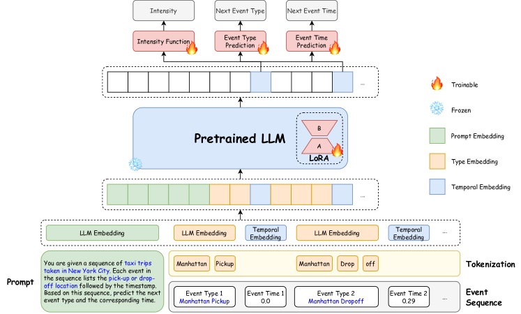
Figure 1: The TPP-LLM framework for event sequence prediction. Textual event descriptions are tokenized and processed through a pretrained LLM to capture semantic information, while temporal embeddings represent event timings. These are combined and passed through the LLM to generate history vectors. Low-rank adaptation (LoRA) optimizes the model for event sequences, with a trainable intensity function and head layers for predicting next events.

2 Related Work

Neural Temporal Point Processes. Recent advances in neural temporal point processes (TPPs) have introduced models that leverage deep learning techniques to capture complex temporal dependencies and event interactions. Many of these models use recurrent neural networks (RNNs) (Hochreiter, 1997) or self-attention mechanisms (Vaswani et al., 2017) to model event intensities based on event history. For example, RMTPP (Du et al., 2016) and NHP (Mei & Eisner, 2017) use RNNs to learn temporal influences, while more recent approaches like SAHP (Zhang et al., 2020) and THP (Zuo et al., 2020) utilize self-attention to capture long-term dependencies. Other models, such as those based on neural ODEs (Chen et al., 2020), normalizing flows (Shchur et al., 2019), attention mechanisms (Yang et al., 2022), diffusion processes (Yuan et al., 2023), meta learning (Bae et al., 2023), and Mamba models (Gao et al., 2024), offer flexible and high-fidelity modeling of discrete events in continuous time. These methods have significantly improved the performance of TPPs by modeling complex interactions and dynamic event relationships.

Large Language Models for Event Sequences. Recent work has explored integrating large language models (LLMs) into event sequence prediction tasks (Jin et al., 2023b). Shi et al. (2024) propose LAMP, a framework that leverages LLMs for abductive reasoning to improve event sequence prediction. Xue et al. (2023b) introduce PromptTPP, which incorporates continual learning into neural temporal point processes to enable adaptive and efficient learning of streaming event sequences. Song et al. (2024) present LaTee, a model utilizing an amortized expectation-maximization framework with logic trees as latent variables and a learnable GFlowNet to generate logic tree samples for more effective event reasoning.

3 Preliminaries

In this section, we introduce the necessary background on temporal point processes and their extensions using neural networks for modeling complex event sequences.

3.1 Temporal Point Processes

Temporal point processes (TPPs) (Hawkes, 1971; Laub et al., 2015) are a class of stochastic processes used to model the occurrence of discrete events over continuous time. A marked TPP extends this framework by associating each event with both a time of occurrence and a type (mark), making it highly applicable in domains where understanding both event types and their timing is critical.

In a marked TPP, a sequence of events over an observation window $[0,T]$ is represented as: $\mathcal{S}=\{(t_{1},k_{1}),(t_{2},k_{2}),\dots,(t_{n},k_{n})\}$, where $t_{i}$ represents the time of the $i$-th event and $k_{i}\in\mathcal{K}$ represents the corresponding event type from a discrete set $\mathcal{K}=\{1,2,\dots,K\}$. The goal is to model the probability of the next event’s time and type, given the history of previous events.

The key function in a TPP is the conditional intensity function $\lambda(t,k|\mathcal{H}_{t})$, which defines the instantaneous rate at which an event of type $k$ occurs at time $t$, conditioned on the history $\mathcal{H}_{t}$. Formally, it is defined as:

$$\lambda(t,k|\mathcal{H}_{t})=\lim_{\Delta t\to 0}\frac{\mathbb{E}[N(t+\Delta t)-N(t)|\mathcal{H}_{t}]}{\Delta t},$$ (1)

where $\mathcal{H}_{t}=\{(t_{j},k_{j}):t_{j}<t\}$ represents the history of previous events up to time $t$, and $N(t)$ is the counting process representing the number of events that have occurred up to time $t$. This intensity function provides the expected number of events occurring in a small time interval $[t,t+\Delta t)$, conditioned on the past. The joint probability density $p(t,k|\mathcal{H}_{t})$ represents the likelihood of the next event occurring at time $t$ with type $k$, conditioned on the history $\mathcal{H}_{t}$. It is expressed as: $p(t,k|\mathcal{H}_{t})=\lambda(t,k|\mathcal{H}_{t})\exp\left(-\int_{t_{i}}^{t}\sum_{k^{\prime}\in\mathcal{K}}\lambda(s,k^{\prime}|\mathcal{H}_{s})\,\mathrm{d}s\right)$, where the integral accounts for no events occurring between the last event at $t_{i}$ and the current time $t$, capturing both event timing and type dependencies.

To evaluate the fit of a TPP model to observed data, the log-likelihood function is commonly used. The log-likelihood of observing a sequence of events $\mathcal{S}$ under a marked TPP is given by:

$$\mathcal{L}(\mathcal{S})=\sum_{i=1}^{n}\log\lambda(t_{i},k_{i}|\mathcal{H}_{t_{i}})-\int_{0}^{T}\sum_{k\in\mathcal{K}}\lambda(t,k|\mathcal{H}_{t})\,\mathrm{d}t,$$ (2)

where the first term sums over the observed events, and the second term integrates over time and all possible event types $k$ to account for the likelihood of no events occurring between observations.

3.2 Neural Temporal Point Processes

Recent advances in TPPs have introduced neural-based models that leverage the representational power of deep learning to capture complex event sequences. These models typically parameterize the conditional intensity function $\lambda(t,k|\mathcal{H}_{t})$ using neural networks, enabling them to learn both temporal dependencies and event type distributions directly from data.

In neural TPPs, for each event $(t_{i},k_{i})$, an embedding $\bm{e}_{i}\in\mathbb{R}^{D}$ is computed through embedding layers based on the event time $t_{i}$ and the event type $k_{i}$. The hidden state $\bm{h}_{t}$, which represents the history up to time $t$, is then updated based on the current event’s embedding and the previous hidden state $\bm{h}_{i-1}$. This update can be formulated as: $\bm{h}_{i}=f_{\text{update}}(\bm{h}_{i-1},\bm{e}_{i})$, where $f_{\text{update}}$ is a neural network, often implemented as a recurrent neural network (RNN) (Hochreiter, 1997) or a more advanced attention-based mechanism (Vaswani et al., 2017). With the updated hidden state $\bm{h}_{i}$, the next event time $t_{i+1}$ and event type $k_{i+1}$ are sampled from the probability distribution conditioned on $\bm{h}_{i}$: $t_{i+1},k_{i+1}\sim P(t_{i+1},k_{i+1}|\bm{h}_{i})$. Different neural TPP models employ various architectures for the state update function $f$. Early approaches (Du et al., 2016; Mei & Eisner, 2017) use RNNs to capture temporal dependencies between events, while more recent models (Zhang et al., 2020; Zuo et al., 2020; Yang et al., 2022) replace the recurrent structure with attention-based layers, allowing for better long-range interactions. These neural-based methods enhance the flexibility of TPPs, learning event dependencies from complex datasets in a data-driven manner.

4 Methodology

In this section, we introduce our proposed framework, TPP-LLM, which leverages large language models (LLMs) to model temporal point processes (TPPs). TPP-LLM, illustrated in Figure 1, integrates pretrained LLMs to capture the semantic richness of event types and employs temporal embeddings to handle the temporal dynamics of event sequences.

4.1 Event and Prompt Embeddings

TPP-LLM models the sequence of events $\mathcal{S}=\{(t_{1},k_{1}),(t_{2},k_{2}),\dots,(t_{n},k_{n})\}$, where each event $e_{i}$ consists of a time $t_{i}$ and a corresponding event type $k_{i}$. Unlike conventional TPP models, which use discrete event types, TPP-LLM directly processes the textual descriptions of event types using a pretrained LLM. This enables the model to capture richer semantic information from the event text while learning temporal dependencies.

The event type $k_{i}$ is represented as a sequence of tokens. Let $x_{i}=\{x_{i,1},x_{i,2},\dots,x_{i,L_{i}}\}$ be the sequence of tokens for event type $k_{i}$, where $L_{i}$ is the length of the tokenized event type. Each token $x_{i,j}$ is mapped to an embedding $\bm{x}_{i,j}\in\mathbb{R}^{D}$ through the pretrained LLM’s embedding layer $\bm{E}\in\mathbb{R}^{V\times D}$, where $V$ is the vocabulary size and $D$ is the embedding dimension. In addition to the event type representation, TPP-LLM incorporates a temporal embedding to capture the time dynamics. Each event time $t_{i}$ is mapped to a temporal embedding $\bm{t}_{i}\in\mathbb{R}^{D}$ using an embedding layer: $\bm{t}_{i}=f_{\text{temporal}}(t_{i})$, where $f_{\text{temporal}}$ can be a linear layer or a positional encoding. In this research, we utilize the temporal positional encoding (Zuo et al., 2020):

$$[\bm{t}_{i}]_{j}=\begin{cases}\cos\left(\frac{t_{j}}{10000^{(i-1)/D}}\right),&\text{when }i\text{ is odd},\\ \sin\left(\frac{t_{j}}{10000^{i/D}}\right),&\text{when }i\text{ is even}.\end{cases}$$ (3)

Other encoding methods (Zhang et al., 2020; Gao & Dai, 2024) can also be applied.

To model the joint dynamics of event types and their timing, we combine the event type representation $\bm{X}_{i}=[\bm{x}_{i,1},\bm{x}_{i,2},\dots,\bm{x}_{i,L_{i}}]\in\mathbb{R}^{L_{i}\times D}$ with the temporal embedding $\bm{t}_{i}\in\mathbb{R}^{D}$. The concatenated representation for each event $(t_{i},k_{i})$ is given by: $\bm{E}_{i}=\left[\bm{x}_{i,1},\bm{x}_{i,2},\dots,\bm{x}_{i,L_{i}},\bm{t}_{i}\right]$ or $\left[\bm{t}_{i},\bm{x}_{i,1},\bm{x}_{i,2},\dots,\bm{x}_{i,L_{i}}\right]\in\mathbb{R}^{(L_{i}+1)\times D}$, depending on the event type and time order.

In addition to the event-specific embeddings, we also prepend a prompt as a sequence of tokens, which is similarly transformed into embeddings via the LLM’s embedding layer: $\bm{P}=[\bm{p}_{1},\bm{p}_{2},\dots,\bm{p}_{L_{p}}]\in\mathbb{R}^{L_{p}\times D}$. The prompt embeddings, along with the concatenated event type and temporal embeddings, form a unified sequence of embeddings: $\bm{X}=[\bm{P},\bm{E}_{1},\bm{E}_{2},\dots,\bm{E}_{n}]\in\mathbb{R}^{(L_{p}+\sum_{i}L_{i}+n)\times D}$, where $\bm{P}$ represents the prompt embeddings and $\bm{E}_{i}$ represents the event type and time embeddings of one event.

4.2 History Vectors and Intensity Function

The entire sequence $\bm{X}$ is then passed through the LLM to obtain contextualized hidden states for each token: $\bm{H}=\text{LLM}(\bm{X})$. After processing, we extract the hidden states corresponding to the last embedding vector of each event. For example, the hidden state of the event $i$ is $\bm{h}_{i}=\bm{H}_{L_{P}+\sum_{j\leq i}L_{j}+i}\in\mathbb{R}^{H}$. The selected hidden states $\bm{h}_{i}$ represent the event history up to time $t_{i}$ (inclusive): $\mathcal{H}_{t_{i}}^{\prime}=\{(t_{j},k_{j}):t_{j}\leq t_{i}\}$. These history vectors are then used for modeling TPPs.

In our model, the intensity function is parameterized using the history vector $\bm{h}_{i}$, which encodes the event history from the initial time to time $t_{i}$. To compute the intensity function between $t_{i}$ and $t_{i+1}$, we apply the linear transformation to the hidden state $\bm{h}_{i}$. For the event type $k$, the intensity function (Zuo et al., 2020; Gao & Dai, 2024) is modeled as:

$$\lambda_{k}(t|\mathcal{H}_{t})=\lambda(t,k|\mathcal{H}_{t})=f_{k}(\alpha_{k}(t-t_{i})+\bm{w}_{k}^{\mathsf{T}}\bm{h}_{i}+b_{k}),$$ (4)

where $f_{k}=\log(1+\exp(x))$ is the softplus function, $\alpha_{k}\in\mathbb{R}$, $\bm{w}_{k}\in\mathbb{R}^{H}$, and $b_{k}\in\mathbb{R}$ are the learnable parameters. The softplus activation ensures the intensity function is non-negative.

4.3 Event Prediction

For each event $(t_{i},k_{i})$, the history vector $\bm{h}_{i}$ from the LLM output encodes the event history $\mathcal{H}_{t_{i}}$, which includes both the event type and temporal dynamics up to time $t_{i}$. Following previous research (Zuo et al., 2020; Gao & Dai, 2024), we utilize this hidden representation to predict both the next event type $k_{i+1}$ and time $t_{i+1}$ through separate layers. To predict the event type, we apply a linear layer followed by a softmax activation to the hidden state $\bm{h}_{i}$, mapping it to a probability distribution over the possible event types: $\hat{\bm{p}}_{i+1}=\hat{\bm{p}}(k_{i+1}|\mathcal{H}_{t_{i}}^{\prime})=\text{softmax}(\bm{W}_{\text{type}}\bm{h}_{i}+\bm{b}_{\text{type}})$, where $\bm{W}_{\text{type}}\in\mathbb{R}^{K\times H}$ and $\bm{b}_{\text{type}}\in\mathbb{R}^{K}$ are the weights and bias of the linear layer, $K$ is the number of event types, and $H$ is the hidden state dimension. The predicted event type $\hat{k}_{i+1}$ is predicted as the type with the maximum probability: $\hat{k}_{i+1}=\arg\max_{k}\hat{\bm{p}}_{i+1}$. Similarly, to predict the next event time, we apply another linear layer to the hidden state $\bm{h}_{i}$, producing a scalar value that represents the next time: $\hat{t}_{i+1}=\bm{w}_{\text{time}}^{\mathsf{T}}\bm{h}_{i}+b_{\text{time}}$, where $\bm{w}_{\text{time}}\in\mathbb{R}^{H}$ and $b_{\text{time}}\in\mathbb{R}$ are the weights and bias for this layer.

4.4 Fine-Tuning

To efficiently adapt the pretrained LLM to the TPP task, we employ low-rank adaptation (LoRA) (Hu et al., 2021), a parameter-efficient fine-tuning (PEFT) (Liu et al., 2022) method. Instead of fine-tuning all the parameters of the LLM, low-rank matrices are introduced to LLM weights. Specifically, we modify the weight matrix of one target module: $W^{\prime}=W+BA$, where $W$ is the original weight, and $A$, $B$ are learnable low-rank matrices. By fine-tuning only these low-rank matrices, we significantly reduce the number of trainable parameters, making the adaptation more efficient without compromising performance. In addition to LoRA, other PEFT methods (Liu et al., 2022; Zhang et al., 2023) can also be applied to further optimize the fine-tuning process.

To fine-tune the LLM alongside the additional head layers, we define a combined loss function that includes the log-likelihood of observed events, event type prediction loss, and event time prediction loss. The likelihood function Equation 2 based on the conditional intensity function is adapted to:

$$\mathcal{L}(\mathcal{S})=\sum_{i=1}^{n}\log\lambda(t_{i},k_{i}|\mathcal{H}_{t_{i}})-\int_{t_{1}}^{t_{n}}\sum_{k\in\mathcal{K}}\lambda(t,k|\mathcal{H}_{t})\,\mathrm{d}t,$$ (5)

where the non-event integral can be computed by Monte Carlo or numerical integration methods (Zuo et al., 2020). The event type loss is defined as the cross-entropy between true and predicted event types: $\mathcal{L}_{\text{type}}(\mathcal{S})=\sum_{i=2}^{n}-\bm{k}_{i}^{\mathsf{T}}\log(\hat{\bm{p}}_{i})=\sum_{i=2}^{n}-\log([\hat{\bm{p}}_{i}]_{k_{i}})$, where $\bm{k}_{i}$ is the one-hot encoding for the ground-truth $k_{i}$. The event time loss is defined as the mean squared error between true and predicted event times: $\mathcal{L}_{\text{time}}(\mathcal{S})=\sum_{i=2}^{n}\left(t_{i}-\hat{t}_{i}\right)^{2}$. The training objective is defined as the sum of the negative log-likelihood, along with the event type and time losses, over all sequences $\mathcal{S}_{i}$:

$$\sum_{i=1}^{N}\ell(\mathcal{S}_{i})=\sum_{i=1}^{N}\left(-\mathcal{L}(\mathcal{S}_{i})+\beta_{\text{type}}\mathcal{L}_{\text{type}}(\mathcal{S}_{i})+\beta_{\text{time}}\mathcal{L}_{\text{time}}(\mathcal{S}_{i})\right),$$ (6)

where $\beta_{\text{type}}$ and $\beta_{\text{time}}$ are coefficients for the event type and time losses.

5 Experiments

In this section, we present the experimental evaluation of our proposed TPP-LLM model. We detail the datasets, prompts used, baseline models, experimental settings, results, and ablation analysis.

5.1 Datasets

We conduct experiments on five real-world datasets: Stack Overflow, Chicago Crime, NYC Taxi Trip, U.S. Earthquake, and Amazon Review. Their statistics are shown in Table 1. The datasets span various applications and are widely used in prior TPP research, making them well-suited for evaluating the performance of our model. However, since the currently available versions lack the corresponding event type texts required by TPP-LLM, we preprocess data to include these critical textual descriptions. These diverse datasets allow us to assess the model’s generalization capabilities across different domains, handling sequences with varying lengths, event types, and temporal resolutions. More detailed information is available in Appendix A.

Table 1: Datasets statistics overview for event sequences.

Dataset	# of Types	# of Events	# of Seq.	Avg. Seq. Length	Time Unit
Stack Overflow	25	187,836	3,336	56.31	month
Chicago Crime	20	202,333	4,033	50.17	month
NYC Taxi Trip	8	362,374	2,957	122.55	hour
U.S. Earthquake	3	29,521	3,009	9.81	day
Amazon Review	18	127,054	2,245	56.59	week

5.2 Prompt Design

We design the prompt to provide a structured guide for the model, helping it understand the task and the sequence of events effectively. The prompt includes essential details such as the sequence context and specifics about event types, allowing the model to focus on the key components it needs to process for accurate predictions. The general structure of the prompt is as follows: “{Sequence Description} {Event Description} {Task Description}” with the task description tailored to the prediction task. When event type precedes time in the embedding sequences, the task is framed as: “Based on this sequence, predict the next event type and the corresponding time.” Alternatively, when event time comes first, the task becomes: “Based on this sequence, predict the next event time and the corresponding type.” The specific sequence and event descriptions for datasets used in our experiments are listed in Appendix C.

5.3 Baselines and Evaluation Metrics

We compare our model, TPP-LLM, with several state-of-the-art (SOTA) baselines to evaluate its performance across different tasks. The baselines include the Neural Hawkes Process (NHP) (Mei & Eisner, 2017), Self-Attentive Hawkes Process (SAHP) (Zhang et al., 2020), Transformer Hawkes Process (THP) (Zuo et al., 2020), and Attentive Neural Hawkes Process (AttNHP) (Yang et al., 2022). These models represent leading approaches in neural TPP modeling. Detailed descriptions of the baselines are provided in Appendix B.

To assess model performance, we use the following evaluation metrics: The log-likelihood measures how well the model fits the observed event sequence $\mathcal{S}$, which is computed as Equation 5 with the intensity function. Accuracy is used to evaluate the event type prediction, measuring the proportion of correctly predicted event types: $\text{Accuracy}=\frac{1}{n}\sum_{i=1}^{n}\mathds{1}(k_{i}=\hat{k}_{i})$, where $k_{i}$ is the true event type, $\hat{k}_{i}$ is the predicted event type, and $\mathds{1}$ is the indicator function. Root mean squared error (RMSE) is used to measure the error in predicting the event times. It is calculated as: $\text{RMSE}=\sqrt{\frac{1}{n}\sum_{i=1}^{n}(t_{i}-\hat{t}_{i})^{2}}$, where $t_{i}$ is the true event time and $\hat{t}_{i}$ is the predicted event time.

5.4 Experimental Setup

We conduct experiments using two foundation models for TPP-LLM: TinyLlama-1.1B-Chat-v1.0 (Zhang et al., 2024a) and Gemma-2-2B-IT (Team et al., 2024), both of which are quantized to 4-bit precision (Dettmers et al., 2024) for efficient GPU memory usage. To capture temporal dynamics, we use temporal positional encoding (Zuo et al., 2020), and event type embeddings are processed first, followed by the temporal embedding for each event. The non-event integral term in the log-likelihood is handled using Monte Carlo integration (Zuo et al., 2020) with 20 samples per time interval, applied consistently across all models. For fine-tuning, we employ LoRA (Hu et al., 2021) by adapting weight matrices in attention modules, with dropout applied but without bias. The Adam optimizer (Kingma, 2014) is used for optimizing both the LoRA layers and prediction layers. Baselines implemented in the EasyTPP framework (Xue et al., 2023a) are utilized, with hyperparameters adapted from it for a fair comparison. Experiments results are averaged over five runs with early stopping, and additional hyperparameters are provided in Appendix D. We utilize a single NVIDIA A10 or A100 GPU for baselines and a single H100 GPU for TPP-LLM.

5.5 Experiment Results

We evaluate TPP-LLM against baselines across five real-world datasets. Two TPP-LLM models are included: TPP-Llama (TinyLlama-1.1B-Chat-v1.0) and TPP-Gemma (Gemma-2-2B-IT).

Log-Likelihood Performance. In terms of log-likelihood (Table 2), TPP-LLM models (TPP-Llama and TPP-Gemma) demonstrate competitive performance across most datasets. TPP-Llama achieves the best performance on Stack Overflow, while AttNHP outperforms all models on Chicago Crime, NYC Taxi Trip, and Amazon Review. However, TPP-LLM models still perform strongly, with ranking second on most datasets, except for U.S. Earthquake, where SAHP achieves the top score. These results highlight TPP-LLM’s ability to model complex event sequences effectively, particularly benefiting from the LLM’s ability to capture event semantics. Despite being outperformed on some datasets, TPP-LLM models remain highly competitive overall.

Table 2: Performance comparison of log-likelihood across different datasets.

Model	StackOverflow	Crime	Taxi	Earthquake	Amazon
NHP	-2.005	-2.604	0.366	-0.450	-1.196
SAHP	-6.320	-6.069	-0.228	0.193	-4.201
THP	-1.877	-2.493	0.217	-0.513	-1.083
AttNHP	-1.798	-2.432	0.446	-0.481	-0.959
TPP-Llama	-1.777	-2.451	0.271	-0.475	-1.011
TPP-Gemma	-1.785	-2.480	0.332	-0.479	-1.075

Event Type Prediction Accuracy. For next event type prediction accuracy (Table 3 and Figure 2), TPP-LLM outperforms or matches the performance of baselines across all datasets. TPP-Llama achieves the highest accuracy on Stack Overflow and Amazon Review, while TPP-Gemma excels on NYC Taxi Trip and U.S. Earthquake. Both variants demonstrate substantial improvements over other baselines, particularly when dealing with datasets like Stack Overflow and Amazon Review, where rich event-type semantics can be leveraged by LLMs to improve prediction accuracy. This highlights TPP-LLM’s capacity to integrate event text information into the prediction process, providing a clear advantage over traditional TPP models.

Table 3: Performance comparison of next event type prediction accuracy and event time prediction RMSE across different datasets.

Model	StackOverflow	Crime	Taxi	Earthquake	Amazon
NHP	42.18%/0.629	25.20%/0.736	90.78%/0.960	62.58%/0.389	65.97%/0.721
SAHP	38.63%/0.588	21.39%/0.691	88.02%/0.881	60.11%/0.271	65.93%/0.662
THP	43.81%/0.629	26.70%/0.745	90.85%/0.924	62.39%/0.377	68.56%/0.733
AttNHP	39.12%/0.581	26.97%/0.679	83.76%/0.904	61.87%/0.386	68.90%/0.658
TPP-Llama	44.20%/0.477	26.86%/0.562	91.37%/0.884	62.70%/0.288	69.22%/0.580
TPP-Gemma	43.94%/0.474	24.54%/0.565	91.46%/0.840	63.12%/0.286	67.71%/0.578

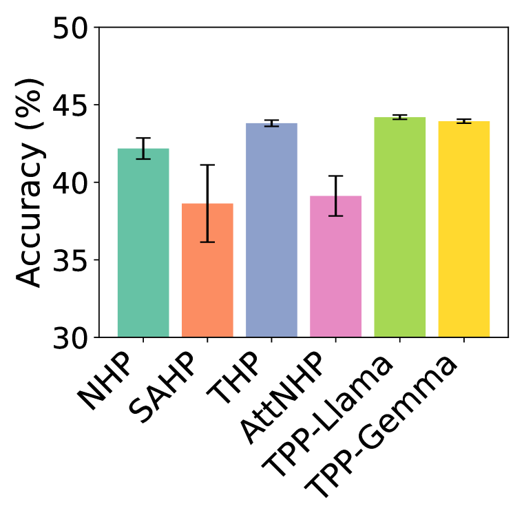
(a) Stack Overflow

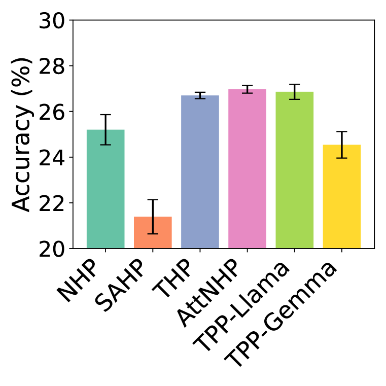
(b) Chicago Crime

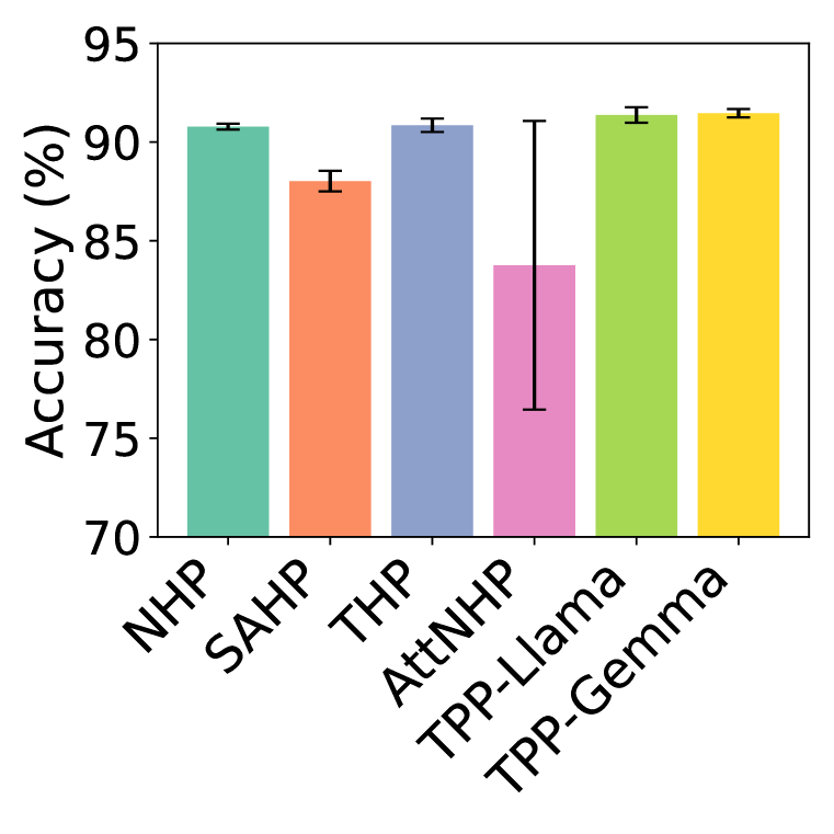
(c) NYC Taxi Trip

(d) U.S. Earthquake

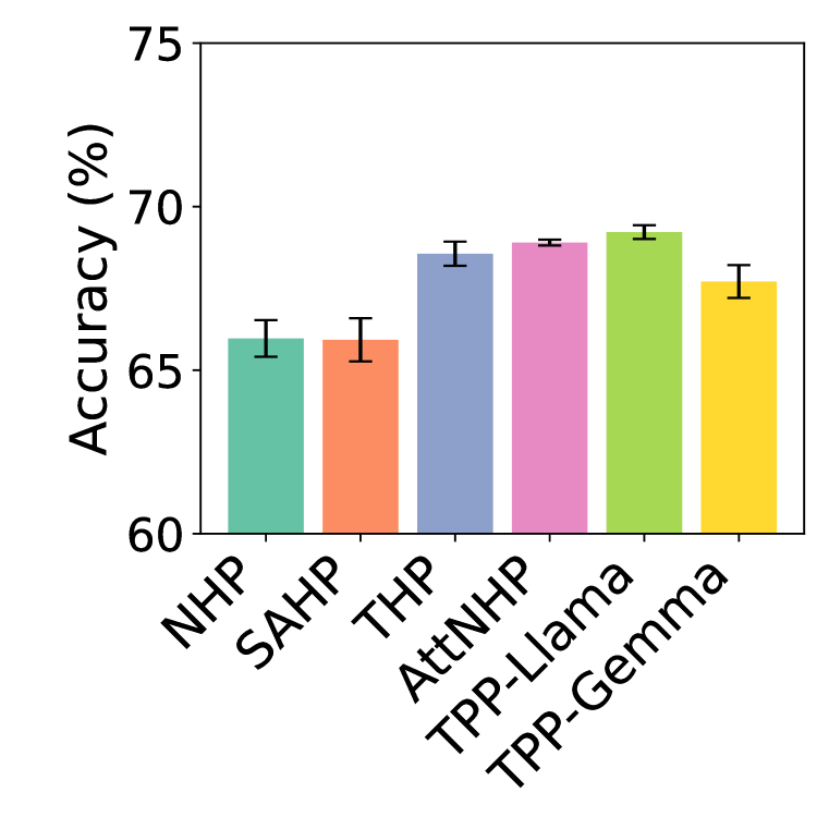
(e) Amazon Review

Figure 2: Performance comparison of next event type prediction accuracy across five different datasets. Each subplot shows the accuracy of six models with error bars.

Event Time Prediction RMSE. When evaluating next event time prediction (Table 3 and Figure 3), TPP-LLM once again delivers strong results. TPP-Gemma achieves the lowest RMSE on Stack Overflow, NYC Taxi Trip, and Amazon Review , while TPP-Llama performs best on Chicago Crime. Both variants significantly outperform baselines, particularly in datasets like Stack Overflow, Chicago Crime, and Amazon Review, where temporal patterns are less regular. This suggests that the LLM-based temporal embeddings in TPP-LLM are effective at capturing temporal dynamics, leading to more accurate event time predictions.

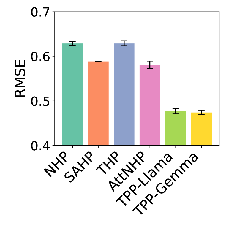
(a) Stack Overflow

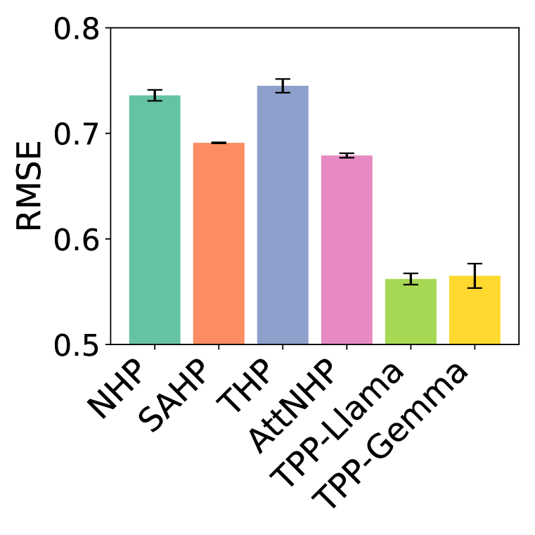
(b) Chicago Crime

(c) NYC Taxi Trip

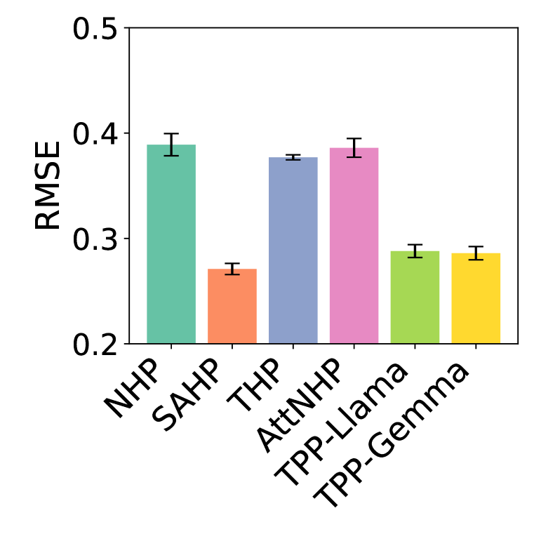
(d) U.S. Earthquake

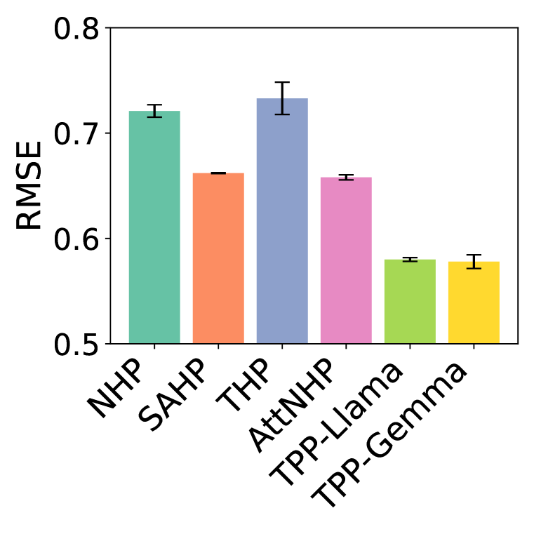
(e) Amazon Review

Figure 3: Performance comparison of next event time prediction RMSE across five different datasets. Each subplot shows the RMSE of six models with error bars.

Overall, TPP-LLM demonstrates strong and consistent performance across all datasets. The inclusion of LLMs for event text processing and understanding allows the model to utilize richer contextual information, leading to better event type prediction accuracy. Additionally, the integration of temporal embeddings helps capture complex temporal dependencies, reflected in the model’s strong RMSE performance for event time predictions. The results confirm that TPP-LLM is an effective and adaptable model for various TPP tasks, achieving leading performance in real-world scenarios.

5.6 Few-Shot Learning

In the few-shot experiments using only 2% of the training data, TPP-LLM models (TPP-Llama and TPP-Gemma) perform strongly across datasets. For log-likelihood (Table 4), TPP-Llama excels on Stack Overflow and Amazon Review, while TPP-Gemma leads on NYC Taxi Trip. AttNHP performs best on Chicago Crime and U.S. Earthquake, with TPP-Llama remaining competitive. In terms of next event type accuracy (Table 5), TPP-Gemma dominates on Stack Overflow, NYC Taxi Trip, and Amazon Review, while TPP-Llama tops U.S. Earthquake. Both TPP-LLM models significantly outperform baselines like NHP and SAHP. For next event time RMSE (Table 5), TPP-Gemma leads on Stack Overflow and Chicago Crime, with SAHP and NHP showing competitive results on other datasets. These findings highlight TPP-LLM’s strong adaptability in few-shot scenarios, effectively leveraging pretrained knowledge.

Table 4: Performance comparison of log-likelihood across different datasets on the 2% training set.

Model	StackOverflow	Crime	Taxi	Earthquake	Amazon
NHP	-6.515	-6.202	-1.236	-0.697	-4.106
SAHP	-6.839	-6.301	-1.173	-0.615	-4.567
THP	-2.683	-2.926	-0.878	-0.625	-1.768
AttNHP	-2.070	-2.594	-0.670	-0.521	-1.474
TPP-Llama	-2.026	-2.668	-0.098	-0.539	-1.469
TPP-Gemma	-2.068	-2.716	0.051	-0.600	-1.630

Table 5: Performance comparison of next event type prediction accuracy and event time prediction RMSE across different datasets on the 2% training set.

Model	StackOverflow	Crime	Taxi	Earthquake	Amazon
NHP	35.23%/0.587	8.27%/0.692	87.70%/0.898	60.36%/0.482	65.08%/0.659
SAHP	37.12%/0.589	6.72%/0.692	45.53%/0.895	59.84%/0.374	65.33%/0.666
THP	35.51%/0.783	19.87%/0.875	46.15%/0.909	54.09%/0.388	65.33%/0.712
AttNHP	41.26%/0.635	25.23%/0.726	47.95%/0.911	61.70%/0.374	65.33%/0.718
TPP-Llama	41.07%/0.567	22.92%/0.647	90.13%/1.118	61.93%/0.613	65.33%/0.833
TPP-Gemma	41.26%/0.514	20.84%/0.604	90.58%/1.103	61.84%/0.538	65.42%/0.683

5.7 Ablation Studies

To understand the contribution of different components in TPP-LLM, we conduct a series of ablation studies. By systematically removing or altering key parts of the model, we analyze how each element affects overall performance and identify which configurations lead to the best results.

5.7.1 Foundation Models

The performance comparison in Table 6 shows the impact of different LLMs on TPP-LLM’s performance. TinyLlama-1.1B-Chat-v1.0 and TinyLlama-1.1B-Intermediate show similar log-likelihood and accuracy scores, with Chat slightly outperforming on next event type prediction for Stack Overflow and U.S. Earthquake. Gemma-2-2B-IT achieves the best RMSE for event time prediction on NYC Taxi Trip and U.S. Earthquake, highlighting its strength in modeling temporal dynamics. Overall, both TinyLlama and Gemma perform competitively, with each excelling in different metrics. The consistent performance across models underscores the robustness of TPP-LLM.

Table 6: Performance comparison of log-likelihood, next event type prediction accuracy, and next event time prediction RMSE across different datasets with various foundation models.

Foundation Model	StackOverflow	Taxi	Earthquake
TinyLlama-1.1B-Intermediate	-1.777/44.17%/0.477	0.313/91.56%/0.847	-0.476/62.65%/0.299
TinyLlama-1.1B-Chat-v1.0	-1.777/44.20%/0.477	0.271/91.37%/0.884	-0.475/62.70%/0.288
Gemma-2-2B	-1.787/44.09%/0.475	0.334/91.52%/0.841	-0.481/62.45%/0.299
Gemma-2-2B-IT	-1.785/43.94%/0.474	0.332/91.46%/0.840	-0.479/63.12%/0.286

5.7.2 Temporal Embeddings

As shown in Table 7, the choice of embedding type and order affects model performance. Positional encoding generally outperforms linear embedding across most metrics. When event time embeddings are processed first, positional encoding achieves the best next event type prediction accuracy and competitive RMSE values. Linear embedding also performs well, with the best log-likelihood on U.S. Earthquake when event time comes first. The results suggest that processing event time before type improves event type prediction, while placing time last enhances time prediction accuracy. These findings highlight the importance of embedding order in model design.

Table 7: Performance comparison of log-likelihood, next event type prediction accuracy, and next event time prediction RMSE across different datasets with various temporal embeddings.

Embedding	First	StackOverflow	Earthquake
Positional	Event Type	-1.777/44.20%/0.477	-0.475/62.70%/0.288
Positional	Event Time	-1.763/44.47%/0.477	-0.475/63.15%/0.307
Linear	Event Type	-1.768/44.15%/0.478	-0.474/62.65%/0.297
Linear	Event Time	-1.768/44.20%/0.477	-0.467/63.01%/0.343

5.7.3 Prompt Settings

Table 8 shows that using a structured prompt (denoted as “Y”) generally improves log-likelihood scores for both TinyLlama models on Stack Overflow, though omitting the prompt (“N”) yields slightly better event type prediction accuracy, especially on U.S. Earthquake. RMSE results are mixed, with prompts providing a small advantage on Stack Overflow but not on U.S. Earthquake. While prompts offer modest log-likelihood gains, their impact on accuracy and RMSE is inconsistent. However, adding prompts enhances the model’s flexibility, particularly for multi-task scenarios.

Table 8: Performance comparison of log-likelihood, next event type prediction accuracy, and next event time prediction RMSE across different datasets with various prompt settings.

Foundation Model	Prompt	StackOverflow	Earthquake
TinyLlama-1.1B-Intermediate	Y	-1.777/44.17%/0.477	-0.476/62.65%/0.299
TinyLlama-1.1B-Intermediate	N	-1.780/44.24%/0.478	-0.471/62.84%/0.291
TinyLlama-1.1B-Chat-v1.0	Y	-1.777/44.20%/0.477	-0.475/62.70%/0.288
TinyLlama-1.1B-Chat-v1.0	N	-1.781/44.11%/0.476	-0.478/62.64%/0.304

5.7.4 Fine-Tuning Settings

Table 9 and Figure 4 illustrate the impact of different LoRA rank configurations on performance. Without fine-tuning (only training the head layers), the model suffers significant drops in log-likelihood and accuracy, highlighting the need for adapting the pretrained LLM. Higher LoRA ranks generally improve results, with rank 32 achieving the best accuracy and log-likelihood on U.S. Earthquake, while lower ranks perform well in terms of log-likelihood and event time prediction. Fine-tuning with LoRA consistently enhances performance, with higher ranks benefiting more complex tasks and lower ranks offering competitive results with less computational cost.

Table 9: Performance comparison of log-likelihood, next event type prediction accuracy, and next event time prediction RMSE across different datasets with various fine-tuning settings.

Fine-Tuning	StackOverflow	Earthquake
None	-1.891/42.43%/0.484	-0.497/62.95%/0.306
LoRA (rank 4)	-1.774/44.18%/0.474	-0.486/62.78%/0.291
LoRA (rank 8)	-1.767/44.20%/0.484	-0.480/63.19%/0.296
LoRA (rank 16)	-1.777/44.20%/0.477	-0.475/62.70%/0.288
LoRA (rank 32)	-1.771/44.39%/0.482	-0.475/63.24%/0.292

(a) Log-likelihood

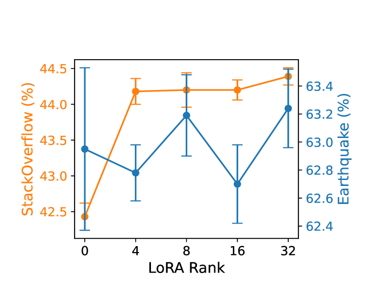
(b) Accuracy

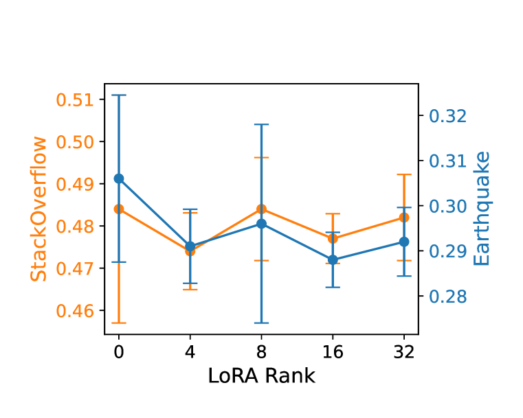
(c) RMSE

Figure 4: Performance comparison of log-likelihood, accuracy, and RMSE for different LoRA ranks with corresponding error bars across the Stack Overflow and U.S. Earthquake datasets.

6 Conclusion

In this paper, we introduced TPP-LLM, a novel framework for modeling temporal point processes (TPP) by leveraging the pretrained knowledge of large language models (LLMs). By integrating LLMs with temporal embeddings, our approach effectively captures both the event semantics and the temporal dynamics of complex event sequences. Through extensive experiments on real-world datasets, we demonstrated that TPP-LLM outperforms state-of-the-art baselines in terms of sequence modeling and next event prediction. Additionally, our ablation studies revealed the contributions of foundation models, temporal embeddings, prompt design, and fine-tuning strategies to overall performance. The robustness of TPP-LLM across diverse datasets and tasks highlights its potential for broader applications in TPP modeling. Future work could explore alternative fine-tuning techniques and embedding strategies, as well as extend this approach to multi-task settings.

Reproducibility Statement

We have made several efforts to ensure the reproducibility of our findings by providing detailed documentation of the experimental setup and methodologies. Detailed descriptions of the datasets used in our experiments, including the preprocessing steps and sequence structure, can be found in Appendix A. The code used for implementing our TPP-LLM model, including the fine-tuning mechanisms, is made available on the GitHub repository. Model architecture details, training procedures, and hyperparameter settings, are provided in Section 5 and Appendix D, enabling the replication of experiments. Additionally, the theoretical foundations of our model are fully explained in Section 3 and 4. This comprehensive approach is intended to facilitate the reproduction of our results and to support further research building on our work.

Appendix A Dataset Details

In this appendix, we provide additional information on the datasets used in our experiments, including detailed preprocessing steps and a breakdown of event types for each dataset.

Table 10: Numbers of sequences in train, validation, and test splits of datasets.

Dataset	# of Seq.	# of Train Seq.	# of Val Seq.	# of Test Seq.
Stack Overflow	3,336	2,668	334	334
Chicago Crime	4,033	3,226	403	404
NYC Taxi Trip	2,957	2,365	296	296
U.S. Earthquake	3,009	2,407	301	301
Amazon Review	2,245	1,796	224	225

A.1 Dataset Summaries

Stack Overflow. We use the badge subset from the Stack Overflow dataset, focusing on non-tag affiliated badges that can be awarded multiple times between January 1, 2022, and December 31, 2023. The dataset includes users with 40-100 badges and badges awarded at least 200 times, resulting in 3,336 sequences with 187,836 events and 25 event types.

Chicago Crime. The Chicago crime dataset covers incidents from January 1, 2022, to December 31, 2023. We focus on the top 20 primary crime types and blocks with 30-120 crime counts. This yields 4,033 sequences with 202,333 events and 20 event types.

NYC Taxi Trip. The NYC taxi dataset spans May 1-7, 2013, excluding trips from or to Staten Island. We keep sequences with 100-160 events, ensuring consecutive events occur within 12 hours. The final dataset contains 2,957 sequences with 362,374 events and 8 location types.

U.S. Earthquake. The United States Earthquake dataset includes earthquakes from January 1, 2020, to December 31, 2023, with events classified as “Large”, “Medium”, or “Small”. We keep sequences with 5-30 events and maximum 24-hour time intervals. The dataset comprises 3,009 sequences with 29,521 events across 3 magnitude types.

Amazon Review. The Amazon review dataset includes reviews from January 1, 2018, to June 30, 2018. After combining same-day reviews in the same category, we focus on users with 40-200 category reviews across 17 categories (plus an “Other” category). This results in 2,245 sequences with 127,054 events across 18 category types.

A.2 Dataset Prepossessing

Stack Overflow. Stack Overflow is a popular question-answering website and online platform where developers and programmers ask and answer technical questions, share knowledge, and solve coding problems collaboratively. We select the badge subset of the Stack Overflow dataset, which includes user IDs, badge names, and others. For data preprocessing methods, we refer to the paper by Du et al. (2016). There are 94 types of non-tag affiliated badges as of March 31, 2024. These badges are designed to recognize a user’s contributions and achievements within the community without being tied to specific tags or categories. We employ badges database schema to parse the data. We select data spanning from January 1, 2022, to December 31, 2023 and keep only the first record if there are duplicates for the same user at the same time due to technical issues. There are 39 badges that can be awarded multiple times by one user. We then select users who have earned between 40 badges and 100 badges and those badges that have been awarded at least 200 times to the selected users. We group the sequences by user. Finally, there are 3,336 sequences with 187,836 events and 25 event types.

Chicago Crime. Chicago crime dataset includes reported crime incidents, excluding murders, that occurred in the City of Chicago. We remove records with missing values in the date, block, or primary crime type fields. Then, we keep only the first record for duplicates with the same block, date, and primary crime type between January 1, 2022 and December 31, 2023. Next, we select the top 20 most frequently occurring primary crime types and choose blocks with crime counts between 30 and 120. We group the sequences by block. Finally, we obtain 4,033 sequences with 202,333 events and 20 event types.

NYC Taxi Trip. NYC taxi trip dataset contains detailed records of taxi trips in New York City, including information such as pick-up and drop-off locations, times, and other relevant details. We first drop any records with missing values and remove duplicate entries, retaining only the first occurrence of each. Additionally, we exclude trips with zero longitude or latitude coordinates. We select data with pickup times spanning from May 1, 2013, to May 7, 2013, and exclude any trips originating from or ending in Staten Island. We divide the sequence based on hack license, ensuring that any two consecutive events are within 12 hours. We select sequences with event counts between 100 and 160. Finally, we obtain 2,957 sequences with 362,374 events and 8 location types.

U.S. Earthquake. The United States earthquake dataset includes information on the time, latitude, longitude, and magnitude of earthquakes spanning from January 1, 2020 to December 31, 2023. We remove records with missing values in the time, coordinate (latitude and longitude), or magnitude fields, and then keep only the first record for duplicates with the same time, coordinate, and magnitude. We divide the sequence based on coordinates with nearest integers, ensuring that any two consecutive events are within 24 hours. If not, a new sequence is started. Then, we only keep the data with Richter magnitude scale (Local magnitude scale, ML) and select sequences with event counts between 5 and 30. We classify the magnitude into three categories, inspired by Zuo et al. (2020). When the magnitude is between 1 (inclusive) and 2 (exclusive), the event is classified as “Medium”; if the magnitude is greater than or equal to 2, it is classified as “Large.” Magnitudes smaller than 1 are classified as “Small.” In total, we identified 3,009 sequences consisting of 29,521 events across three magnitude types.

Amazon Review. Amazon review dataset (Ni et al., 2019) includes reviews, product metadata, and links. We first combine events if a user submits multiple reviews in the same category on the same day. Then, we select data spanning from January 1, 2018 to June 30, 2018. From this dataset, we focus on users who wrote between 40 and 200 category reviews and select the top 17 categories reviewed by these users. We combine all other categories into a single “Other” category. Finally, we obtain 2,245 sequences with 127,054 events across 18 category types.

A.3 Event Types

In this subsection, we provide a detailed mapping of event types to their corresponding textual descriptions for each dataset in Table 11-15. These event types represent the various categories of events modeled in our experiments, allowing the model to capture diverse patterns across different domains.

Table 11: Event IDs and corresponding event types for Stack Overflow dataset.

ID	Event Type	ID	Event Type
0	Yearling	13	Favorite Question
1	Necromancer	14	Populist
2	Enlightened	15	Announcer
3	Guru	16	Booster
4	Nice Question	17	Publicist
5	Good Question	18	Revival
6	Great Question	19	Caucus
7	Nice Answer	20	Constituent
8	Good Answer	21	Custodian
9	Great Answer	22	Steward
10	Popular Question	23	Socratic
11	Notable Question	24	Lifejacket
12	Famous Question

Table 12: Event IDs and corresponding event types for Chicago Crime dataset.

ID	Event Type	ID	Event Type
0	Theft	10	Burglary
1	Weapons Violation	11	Robbery
2	Sex Offense	12	Arson
3	Deceptive Practice	13	Offense Involving Children
4	Motor Vehicle Theft	14	Criminal Sexual Assault
5	Criminal Trespass	15	Interference With Public Officer
6	Criminal Damage	16	Narcotics
7	Battery	17	Stalking
8	Other Offense	18	Public Peace Violation
9	Assault	19	Homicide

Table 13: Event IDs and corresponding event types for NYC Taxi Trip dataset.

ID	Event Type	ID	Event Type
0	Manhattan Pickup	4	Bronx Dropoff
1	Manhattan Dropoff	5	Brooklyn Pickup
2	Queens Dropoff	6	Brooklyn Dropoff
3	Queens Pickup	7	Bronx Pickup

Table 14: Event IDs and corresponding event types for U.S. Earthquake Dataset.

ID	Event Type
0	Large
1	Medium
2	Small

Table 15: Event IDs and corresponding event types for Amazon Review dataset.

ID	Event Type	ID	Event Type
0	Other	9	Office Products
1	Tools and Home Improvement	10	Books
2	Pet Supplies	11	Home and Kitchen
3	Arts Crafts and Sewing	12	Sports and Outdoors
4	Electronics	13	Patio Lawn and Garden
5	Automotive	14	Movies and TV
6	Industrial and Scientific	15	Clothing Shoes and Jewelry
7	Grocery and Gourmet Food	16	Kindle Store
8	Toys and Games	17	Cell Phones and Accessories

Appendix B Baseline Details

Neural Hawkes Process (NHP) (Mei & Eisner, 2017) is a generative model that uses a continuous-time LSTM to dynamically adjust the intensity of multiple event types based on the sequence of past events, enabling accurate predictions of future event types and timings. Self-Attentive Hawkes Process (SAHP) (Zhang et al., 2020) enhances Hawkes processes by using self-attention to model event dynamics, incorporating time intervals into positional encoding, and improving predictive accuracy and interpretability compared to RNN-based models. Transformer Hawkes Process (THP) (Zuo et al., 2020) leverages the self-attention mechanism to efficiently capture long-term dependencies in event sequence data, improving prediction accuracy and likelihood over recurrent neural network-based models. Attentive Hawkes Process (AttNHP) (Yang et al., 2022) replaces LSTM-based architectures with attention-based models to more efficiently capture event sequences and participant embeddings, maintaining or improving prediction accuracy compared to previous neuro-symbolic and attention-based approaches.

Appendix C Prompt Details

In this section, we provide the detailed prompts designed for each dataset, illustrating how the event sequences are structured based on whether the event type or event time appears first. Table 16 outlines the sequence descriptions and event formatting for each dataset.

Table 16: Prompts designed for each dataset, showing how event sequences are structured with either event type first or event time first.

Dataset	Sequence Description	Event Description
		Event Type First	Event Time First
Stack Overflow	You are given a sequence of badge awards earned by a user on the Stack Overflow platform.	Each event in the sequence lists the badge name followed by the timestamp.	Each event in the sequence lists the timestamp followed by the badge name.
Chicago Crime	You are given a sequence of reported crime incidents that occurred in the City of Chicago.	Each event in the sequence lists the crime type followed by the timestamp.	Each event in the sequence lists the timestamp followed by the crime type.
NYC Taxi Trip	You are given a sequence of taxi trips taken in New York City.	Each event in the sequence lists the pick-up or drop-off location followed by the timestamp.	Each event in the sequence lists the timestamp followed by the pick-up or drop-off location.
U.S. Earthquake	You are given a sequence of earthquake events recorded in the United States.	Each event in the sequence lists the magnitude classification (large or small) followed by the timestamp.	Each event in the sequence lists the timestamp followed by the magnitude classification (large or small).
Amazon Review	You are given a sequence of product category reviews written by a user on the Amazon platform.	Each event in the sequence lists the product category followed by the timestamp.	Each event in the sequence lists the timestamp followed by the product category.

Appendix D Model Hyperparameters

This section details the hyperparameters used for the various models in our experiments. Table 17 summarizes the key hyperparameter configurations for each baseline (NHP, SAHP, THP, AttNHP) and our proposed model, TPP-LLM. For TPP-LLM, we include specific settings for LoRA fine-tuning, such as the rank, alpha, and dropout parameters, as well as the target attention modules.

Table 17: Hyperparameter configurations used for various models in the experiments. The hidden size, embedding dimension, and other model structure parameters of TPP-LLM depend on the foundation model.

Hyperparameter	NHP	SAHP	THP	AttNHP	TPP-LLM
hidden_size	64	64	64	64	-
time_emb_size	16	16	16	16	-
num_layers	2	2	2	2	-
num_heads	-	2	2	2	-
batch_size	128	128	128	8	8
max_epoch	10	20	20	8	20
learning_rate	1e-3	1e-3	1e-3	1e-3	5e-4
num_integral_samples	20	20	20	20	20
lora_rank	-	-	-	-	16
lora_alpha	-	-	-	-	16
lora_dropout	-	-	-	-	0.05
target_modules	-	-	-	-	Q, K, V, O
beta_type	-	-	-	-	1
beta_time	-	-	-	-	1

Appendix E Experiment Result Details

E.1 Standard Deviations for Full-Training Results

This subsection reports the standard deviations for log-likelihood (Table 18), next event type prediction accuracy (Table 19), and next event time prediction RMSE (Table 20) from the full-training experiments. These results help assess the consistency of model performance across different datasets.

Table 18: Performance comparison of standard deviations in log-likelihood across different datasets.

Model	StackOverflow	Crime	Taxi	Earthquake	Amazon
NHP	0.0094	0.0134	0.0074	0.0019	0.0236
SAHP	0.0781	0.0140	0.0765	0.0140	0.1167
THP	0.0100	0.0046	0.0794	0.0084	0.0192
AttNHP	0.0095	0.0025	0.0353	0.0070	0.0205
TPP-Llama	0.0137	0.0160	0.0497	0.0075	0.0392
TPP-Gemma	0.0118	0.0098	0.0086	0.0024	0.0380

Table 19: Performance comparison of standard deviations in next event type prediction accuracy across different datasets.

Model	StackOverflow	Crime	Taxi	Earthquake	Amazon
NHP	0.0068	0.0066	0.0015	0.0019	0.0056
SAHP	0.0249	0.0075	0.0052	0.0097	0.0066
THP	0.0020	0.0014	0.0034	0.0035	0.0037
AttNHP	0.0129	0.0017	0.0731	0.0039	0.0009
TPP-Llama	0.0014	0.0033	0.0039	0.0028	0.0021
TPP-Gemma	0.0013	0.0058	0.0021	0.0030	0.0050

Table 20: Performance comparison of standard deviations in next event time prediction RMSE across different datasets.

Model	StackOverflow	Crime	Taxi	Earthquake	Amazon
NHP	0.0048	0.0052	0.0075	0.0105	0.0059
SAHP	0.0003	0.0005	0.0021	0.0053	0.0004
THP	0.0056	0.0065	0.0179	0.0024	0.0153
AttNHP	0.0079	0.0021	0.0054	0.0089	0.0024
TPP-Llama	0.0059	0.0053	0.0490	0.0061	0.0018
TPP-Gemma	0.0047	0.0116	0.0065	0.0063	0.0065

E.2 Standard Deviations for Few-Shot Results

This subsection presents the standard deviations for log-likelihood (Table 21), accuracy (Table 22), and RMSE (Table 23) from the few-shot learning experiments. These values provide insight into how stable the models are when trained on limited data.

Table 21: Performance comparison of standard deviations in log-likelihood performance across different datasets on the 2% training set.

Model	StackOverflow	Crime	Taxi	Earthquake	Amazon
NHP	0.1837	0.0899	0.0299	0.0247	0.2063
SAHP	0.0083	0.0061	0.0098	0.0252	0.0042
THP	0.1024	0.0935	0.3683	0.0288	0.0581
AttNHP	0.0254	0.0056	0.0050	0.0173	0.0231
TPP-Llama	0.0107	0.0367	0.2542	0.0173	0.0889
TPP-Gemma	0.0305	0.0283	0.1136	0.0624	0.1998

Table 22: Performance comparison of standard deviations in next event type prediction accuracy across different datasets on the 2% training set.

Model	StackOverflow	Crime	Taxi	Earthquake	Amazon
NHP	0.0181	0.0636	0.0169	0.0061	0.0069
SAHP	0.0189	0.0728	0.0039	0.0277	0.0003
THP	0.0117	0.0048	0.0002	0.0716	0.0000
AttNHP	0.0014	0.0020	0.0136	0.0077	0.0001
TPP-Llama	0.0022	0.0156	0.0069	0.0036	0.0055
TPP-Gemma	0.0046	0.0101	0.0033	0.0084	0.0055

Table 23: Performance comparison of standard deviations in next event time prediction RMSE across different datasets on the 2% training set.

Model	StackOverflow	Crime	Taxi	Earthquake	Amazon
NHP	0.0012	0.0007	0.0012	0.0265	0.0017
SAHP	0.0005	0.0005	0.0007	0.0196	0.0009
THP	0.1179	0.0806	0.0032	0.0215	0.0602
AttNHP	0.0121	0.0140	0.0042	0.0221	0.0400
TPP-Llama	0.0268	0.0497	0.0942	0.1706	0.1026
TPP-Gemma	0.0211	0.0149	0.1693	0.1511	0.0346

E.3 Standard Deviations for Fine-Tuning Results

This section provides a detailed comparison of standard deviations for log-likelihood (Table 24), event type prediction accuracy (Table 25), and event time RMSE (Table 26) across different fine-tuning settings. Tables below highlight the performance across datasets when using various LoRA ranks and no fine-tuning.

Table 24: Performance comparison of standard deviations in log-likelihood performance across different datasets with various fine-tuning settings.

Fine-Tuning	StackOverflow	Earthquake
None	0.0292	0.0138
LoRA (rank 4)	0.0131	0.0049
LoRA (rank 8)	0.0059	0.0087
LoRA (rank 16)	0.0137	0.0075
LoRA (rank 32)	0.0079	0.0055

Table 25: Performance comparison of standard deviations in next event type prediction accuracy across different datasets with various fine-tuning settings.

Fine-Tuning	StackOverflow	Earthquake
None	0.0019	0.0058
LoRA (rank 4)	0.0018	0.0020
LoRA (rank 8)	0.0024	0.0029
LoRA (rank 16)	0.0014	0.0028
LoRA (rank 32)	0.0012	0.0028

Table 26: Performance comparison of standard deviations in next event time prediction RMSE across different datasets with various fine-tuning settings.

Fine-Tuning	StackOverflow	Earthquake
None	0.0270	0.0185
LoRA (rank 4)	0.0091	0.0082
LoRA (rank 8)	0.0122	0.0220
LoRA (rank 16)	0.0059	0.0061
LoRA (rank 32)	0.0102	0.0076

References

- Achiam et al. (2023) Josh Achiam, Steven Adler, Sandhini Agarwal, Lama Ahmad, Ilge Akkaya, Florencia Leoni Aleman, Diogo Almeida, Janko Altenschmidt, Sam Altman, Shyamal Anadkat, et al. Gpt-4 technical report. arXiv preprint arXiv:2303.08774, 2023.
- Bae et al. (2023) Wonho Bae, Mohamed Osama Ahmed, Frederick Tung, and Gabriel L Oliveira. Meta temporal point processes. arXiv preprint arXiv:2301.12023, 2023.
- Chen et al. (2020) Ricky TQ Chen, Brandon Amos, and Maximilian Nickel. Neural spatio-temporal point processes. arXiv preprint arXiv:2011.04583, 2020.
- Dettmers et al. (2024) Tim Dettmers, Artidoro Pagnoni, Ari Holtzman, and Luke Zettlemoyer. Qlora: Efficient finetuning of quantized llms. Advances in Neural Information Processing Systems, 36, 2024.
- Du et al. (2016) Nan Du, Hanjun Dai, Rakshit Trivedi, Utkarsh Upadhyay, Manuel Gomez-Rodriguez, and Le Song. Recurrent marked temporal point processes: Embedding event history to vector. In Proceedings of the 22nd ACM SIGKDD international conference on knowledge discovery and data mining, pp. 1555–1564, 2016.
- Dubey et al. (2024) Abhimanyu Dubey, Abhinav Jauhri, Abhinav Pandey, Abhishek Kadian, Ahmad Al-Dahle, Aiesha Letman, Akhil Mathur, Alan Schelten, Amy Yang, Angela Fan, et al. The llama 3 herd of models. arXiv preprint arXiv:2407.21783, 2024.
- Gao & Dai (2024) Anningzhe Gao and Shan Dai. Rothp: Rotary position embedding-based transformer hawkes process. arXiv preprint arXiv:2405.06985, 2024.
- Gao et al. (2024) Anningzhe Gao, Shan Dai, and Yan Hu. Mamba hawkes process. arXiv preprint arXiv:2407.05302, 2024.
- Hawkes (1971) Alan G Hawkes. Spectra of some self-exciting and mutually exciting point processes. Biometrika, 58(1):83–90, 1971.
- Hochreiter (1997) S Hochreiter. Long short-term memory. Neural Computation MIT-Press, 1997.
- Hu et al. (2021) Edward J Hu, Yelong Shen, Phillip Wallis, Zeyuan Allen-Zhu, Yuanzhi Li, Shean Wang, Lu Wang, and Weizhu Chen. Lora: Low-rank adaptation of large language models. arXiv preprint arXiv:2106.09685, 2021.
- Jin et al. (2023a) Ming Jin, Shiyu Wang, Lintao Ma, Zhixuan Chu, James Y Zhang, Xiaoming Shi, Pin-Yu Chen, Yuxuan Liang, Yuan-Fang Li, Shirui Pan, et al. Time-llm: Time series forecasting by reprogramming large language models. arXiv preprint arXiv:2310.01728, 2023a.
- Jin et al. (2023b) Ming Jin, Qingsong Wen, Yuxuan Liang, Chaoli Zhang, Siqiao Xue, Xue Wang, James Zhang, Yi Wang, Haifeng Chen, Xiaoli Li, et al. Large models for time series and spatio-temporal data: A survey and outlook. arXiv preprint arXiv:2310.10196, 2023b.
- Kingma (2014) Diederik P Kingma. Adam: A method for stochastic optimization. arXiv preprint arXiv:1412.6980, 2014.
- Laub et al. (2015) Patrick J Laub, Thomas Taimre, and Philip K Pollett. Hawkes processes. arXiv preprint arXiv:1507.02822, 2015.
- Liu et al. (2022) Haokun Liu, Derek Tam, Mohammed Muqeeth, Jay Mohta, Tenghao Huang, Mohit Bansal, and Colin A Raffel. Few-shot parameter-efficient fine-tuning is better and cheaper than in-context learning. Advances in Neural Information Processing Systems, 35:1950–1965, 2022.
- Mei & Eisner (2017) Hongyuan Mei and Jason M Eisner. The neural hawkes process: A neurally self-modulating multivariate point process. Advances in neural information processing systems, 30, 2017.
- Ni et al. (2019) Jianmo Ni, Jiacheng Li, and Julian McAuley. Justifying recommendations using distantly-labeled reviews and fine-grained aspects. In Proceedings of the 2019 conference on empirical methods in natural language processing and the 9th international joint conference on natural language processing (EMNLP-IJCNLP), pp. 188–197, 2019.
- Shchur et al. (2019) Oleksandr Shchur, Marin Biloš, and Stephan Günnemann. Intensity-free learning of temporal point processes. arXiv preprint arXiv:1909.12127, 2019.
- Shchur et al. (2021) Oleksandr Shchur, Ali Caner Türkmen, Tim Januschowski, and Stephan Günnemann. Neural temporal point processes: A review. arXiv preprint arXiv:2104.03528, 2021.
- Shi et al. (2024) Xiaoming Shi, Siqiao Xue, Kangrui Wang, Fan Zhou, James Zhang, Jun Zhou, Chenhao Tan, and Hongyuan Mei. Language models can improve event prediction by few-shot abductive reasoning. Advances in Neural Information Processing Systems, 36, 2024.
- Song et al. (2024) Zitao Song, Chao Yang, Chaojie Wang, Bo An, and Shuang Li. Latent logic tree extraction for event sequence explanation from llms. arXiv preprint arXiv:2406.01124, 2024.
- Team et al. (2024) Gemma Team, Morgane Riviere, Shreya Pathak, Pier Giuseppe Sessa, Cassidy Hardin, Surya Bhupatiraju, Léonard Hussenot, Thomas Mesnard, Bobak Shahriari, Alexandre Ramé, et al. Gemma 2: Improving open language models at a practical size. arXiv preprint arXiv:2408.00118, 2024.
- Vaswani et al. (2017) Ashish Vaswani, Noam Shazeer, Niki Parmar, Jakob Uszkoreit, Llion Jones, Aidan N Gomez, Łukasz Kaiser, and Illia Polosukhin. Attention is all you need. Advances in neural information processing systems, 30, 2017.
- Xue et al. (2023a) Siqiao Xue, Xiaoming Shi, Zhixuan Chu, Yan Wang, Hongyan Hao, Fan Zhou, Caigao JIANG, Chen Pan, James Y Zhang, Qingsong Wen, et al. Easytpp: Towards open benchmarking temporal point processes. In The Twelfth International Conference on Learning Representations, 2023a.
- Xue et al. (2023b) Siqiao Xue, Yan Wang, Zhixuan Chu, Xiaoming Shi, Caigao Jiang, Hongyan Hao, Gangwei Jiang, Xiaoyun Feng, James Zhang, and Jun Zhou. Prompt-augmented temporal point process for streaming event sequence. Advances in Neural Information Processing Systems, 36:18885–18905, 2023b.
- Yang et al. (2022) Chenghao Yang, Hongyuan Mei, and Jason Eisner. Transformer embeddings of irregularly spaced events and their participants. In Proceedings of the Tenth International Conference on Learning Representations (ICLR), 2022.
- Yuan et al. (2023) Yuan Yuan, Jingtao Ding, Chenyang Shao, Depeng Jin, and Yong Li. Spatio-temporal diffusion point processes. In Proceedings of the 29th ACM SIGKDD Conference on Knowledge Discovery and Data Mining, pp. 3173–3184, 2023.
- Zhang et al. (2024a) Peiyuan Zhang, Guangtao Zeng, Tianduo Wang, and Wei Lu. Tinyllama: An open-source small language model. arXiv preprint arXiv:2401.02385, 2024a.
- Zhang et al. (2020) Qiang Zhang, Aldo Lipani, Omer Kirnap, and Emine Yilmaz. Self-attentive hawkes process. In International conference on machine learning, pp. 11183–11193. PMLR, 2020.
- Zhang et al. (2023) Renrui Zhang, Jiaming Han, Chris Liu, Peng Gao, Aojun Zhou, Xiangfei Hu, Shilin Yan, Pan Lu, Hongsheng Li, and Yu Qiao. Llama-adapter: Efficient fine-tuning of language models with zero-init attention. arXiv preprint arXiv:2303.16199, 2023.
- Zhang et al. (2024b) Xiyuan Zhang, Ranak Roy Chowdhury, Rajesh K Gupta, and Jingbo Shang. Large language models for time series: A survey. arXiv preprint arXiv:2402.01801, 2024b.
- Zhao et al. (2023) Wayne Xin Zhao, Kun Zhou, Junyi Li, Tianyi Tang, Xiaolei Wang, Yupeng Hou, Yingqian Min, Beichen Zhang, Junjie Zhang, Zican Dong, et al. A survey of large language models. arXiv preprint arXiv:2303.18223, 2023.
- Zhou et al. (2023) Tian Zhou, Peisong Niu, Liang Sun, Rong Jin, et al. One fits all: Power general time series analysis by pretrained lm. Advances in neural information processing systems, 36:43322–43355, 2023.
- Zuo et al. (2020) Simiao Zuo, Haoming Jiang, Zichong Li, Tuo Zhao, and Hongyuan Zha. Transformer hawkes process. In International conference on machine learning, pp. 11692–11702. PMLR, 2020.