Non-parametric reconstruction of cosmological observables using Gaussian Processes Regression.

Abstract

The current accelerated expansion of the Universe remains ones of the most intriguing topics in modern cosmology, driving the search for innovative statistical techniques. Recent advancements in machine learning have significantly enhanced its application across various scientific fields, including physics, and particularly cosmology, where data analysis plays a crucial role in problem-solving. In this work, a non-parametric regression method with Gaussian processes is presented along with several applications to reconstruct some cosmological observables, such as the deceleration parameter and the dark energy equation of state, in order to contribute with some information that helps to clarify the behavior of the Universe. It was found that the results are consistent with $\Lambda$CDM and the predicted value of the Hubble parameter at redshift zero is $H_{0}=68.798\pm 6.340(1\sigma)\text{ km}\text{ Mpc}^{-1}\text{ s}^{-1}$.

I Introduction

Nowadays it is becoming more common to hear that we are currently living in the Golden Age of Cosmology, whose origin goes back to the early 90’s when the Cosmic Background Explorer (COBE) satellite was launched in order to provide information of the Cosmic Microwave Background Boggess et al. (1992). This event marked the beginning of a series of outstanding discoveries such as the necessity to incorporate the Dark Matter (DM) and Dark Energy (DE) components to account for the structure formation and the current accelerated expansion of the Universe, which later on gave rise to the standard cosmological model or Lambda Cold Dark Matter (LCDM) (more on this model later). This Golden Age is also characterized by the huge amount of observations and data obtained as a result of several world-wide collaborations, such as Planck Akrami et al. (2018), SDSS York et al. (2000), SNLS Astier et al. (2006), DESI Levi et al. (2019), JWST Gardner et al. (2023) and Euclid Laureijs et al. (2011), to mention a few. This was definitely a remarkable achievement since it provided the community with valuable information to work with, but it also came with a set of obstacles, such as how to process and analyze the avalanche of new data. Fortunately, around the same time, a new field of mathematics was starting to grow in strength: Machine Learning.

Machine Learning (ML) is the subfield of Artificial Intelligence dedicated to the mathematical modeling of data. It is a method to find solutions to problems by using computers, which differs from regular programming since the latter takes data and rules to return results. In contrast, ML takes data and results to deduce the rules that relate them. A ML system is said to be trained rather than programmed Chollet (2017). ML can be broadly categorized into three types: supervised, unsupervised, and reinforcement learning Theobald (2017). It can handle a wide variety of problems, but the main goal is to learn the process of mapping inputs into outputs, which can then be used to predict the outputs for new, unseen, inputs. These algorithms have been widely compared against traditional techniques in related fields, obtaining promising results in terms of efficiency and performance in favor of ML Sarker (2021); Ray (2019); Qiu et al. (2016); Mahesh (2020); Dhall et al. (2020). The main advantage of ML algorithms is that they can automate repetitive tasks such as data cleaning and pattern recognition that might require direct human intervention with traditional methods.

On the other hand, in the construction of predictive models, ML is particularly useful for scientific research, since the applications allowed the development of non-parametric models of physical quantities for which their analytical expression is not entirely clear. That is, ML algorithms allow to predict the behavior of some observable quantities, even when an exact model of them is not fully specified müller2016introduction. Some useful and popular supervised learning methods that have been applied to Cosmology are:

Artificial Neural Networks (ANN): Named so because of their analogy to the behavior of the human brain. ANN are made up of layers of sets of units called neurons that individually process data inputs. Each neuron is connected to the others through links with weights that are evaluated by an activation function, discarding the worst options and prioritizing the best ones. ANN are commonly used to solve classification and pattern recognition problems in images, speech, or signals. ANN have also predictive applications in the financial Sewell (2023) or atmospheric Abhishek et al. (2012) sector. The field of Cosmology is no stranger to Neural Networks, just to mention a few examples we have: CosmicNet I Albers et al. (2019) and CosmicNet II Günther et al. (2022), which are used to accelerate Einstein-Boltzmann solvers; physically-informed neural networks as a replacement for numerical solvers for differential equations in cosmological codes Chantada et al. (2022, 2023); a more suited application consists on using ANN directly with data to non-parametically reconstruct certain cosmological quantities such as the Hubble parameter and structure formation through $f\sigma_{8}$ Gómez-Vargas et al. (2023a), deceleration parameter Mukherjee et al. (2022), rotation curves Garcia-Arroyo et al. (2024); on scalar-tensor theories Dialektopoulos et al. (2024); or to test the cosmic distance ladder Mukherjee et al. (2024a); Shah et al. (2024); to emulate functions such as the power spectrum Agarwal et al. (2012, 2014); Costanza et al. (2024) or to speed up computational process Gómez-Vargas and Vázquez (2024); Nygaard et al. (2023); Sikder et al. (2023); Jense et al. (2024), along with Genetic Algorithms Gómez-Vargas et al. (2023b); for an introduction of ANN in Cosmology, see Olvera et al. (2022).

Decision Trees and Random Forests (RF): Essentially, Decision Trees learn a hierarchy of if/else questions and reach an appropriate decision. Decision trees can be used in marketing campaigns Liu and Yang (2022) or diagnosis of diseases Podgorelec et al. (2002) to mention a few examples. Random Forests are based on a set of Decision Trees that are uncorrelated and merged to create more accurate data predictions. These types of algorithms are often used to solve classification problems Pedregosa et al. (2011), which can be of great use in the field of Cosmology. Some examples are: Gravitational Waves’ classification Shah et al. (2023); Baker et al. (2015), joint redshift-stellar mass probability distribution functions Mucesh et al. (2021) and N-body simulations Conceição et al. (2024); Chacón et al. (2022, 2023).

k-Nearest Neighbors (k-NN): This algorithm consists of storing the training dataset and formulating a method that finds the closest data values to make predictions for a new test data point. It is possibly the simplest ML method and has a wide spectrum of applications, such as the creation of customized recommended systems Ji (2021). Given the ease with which k-NN finds groups/agglomerations, its use in cosmology has focused on topics related to structure formation such as galaxy-clustering Banerjee and Abel (2021); Banerjee et al. (2022); Yuan et al. (2023); Wang et al. (2022).

There is another ML technique, which works as the basis for this paper and it is known as Gaussian Process Regression (GPR). Over the last decade, GPR has become particularly popular in cosmology for testing the concordance model Nair et al. (2015); Rana et al. (2017); Mukherjee and Mukherjee (2021); Mukherjee et al. (2023), cosmographic studies Shafieloo et al. (2012a); Mukherjee and Banerjee (2021a); Jesus et al. (2022), reconstruction of parameters that characterize the cosmic expansion Shafieloo et al. (2012b); Mukherjee and Sen (2024); Mukherjee et al. (2024b), reconstructing dark energy Holsclaw et al. (2011); Seikel et al. (2012a); Zhang and Li (2018), constraining spatial curvature Yang and Gong (2021); Dhawan et al. (2021); Mukherjee and Banerjee (2022a), exploring the interaction between dark matter and dark energy Yang et al. (2015); Mukherjee and Banerjee (2021b); Cai et al. (2017); Bonilla et al. (2022); Escamilla et al. (2023), testing modified theories of gravity Zhou et al. (2019); Belgacem et al. (2020); Yang (2021); Levi Said et al. (2021); Bernardo and Levi Said (2021); Dialektopoulos et al. (2024), testing consistency among datasets Keeley et al. (2021), emulating the matter power spectrum Ho et al. (2021), thermodynamic viability analysis Banerjee et al. (2023a, b), probing the cosmic reionization history Adak et al. (2024); Krishak and Hazra (2021); Mukherjee et al. (2024c) and classification and identification of blended galaxies Buchanan et al. (2022); among many other research fields that take advantage of the ML capabilities for analyzing and classifying images, videos and numerical data. For a pedagogical introduction to GPR, one can refer to the Gaussian process website. Over the course of this work a GPR will be defined and then tested by applying it to the prediction of observable quantities in Cosmology. Therefore, the main objective of this work is to provide a basic introduction to Gaussian Processes (GPs) and to present some applications of this method through examples.

II Gaussian Processes

In this section we present some of the relevant concepts before delving into the GPR:

• Random Variable: a variable whose values depend on a random event, could be continuous or discrete, for example: when rolling two 6-sided dice the result will be two outcomes $n_{1}$ and $n_{2}$. In this case, a discrete random variable $X$ can be the sum of the result of rolling both dice, i.e. $X(n_{1},n_{2})=n_{1}+n_{2}$.

• Correlation: also called “dependence”, it is a statistical relationship between two random variables. For example, when comparing the height of a person with that of their parents, in general, it will be observed that the descendants have heights similar to the progenitors, this means that there is a connection or positive correlation between both heights. In general, the presence of consequences does not imply causality.

• Probability distribution: a function that assigns to each event, defined on the random variable, the probability that said event occurs. They can be discrete or continuous. A widely used one is the binomial probability distribution (where there are two possible mutually exclusive events):

  $$P(X=k)=\frac{n!}{k!(n-k)!}p^{k}(1-p)^{k},$$ (1)

  where $k$ is the number of times an event has occurred, $p$ the probability that said event occurs, and $n$ the number of total events.

• Normal distribution: also called Gaussian distribution, it is a type of continuous probability distribution with the form:

  $$f(x)=\frac{1}{\sigma\sqrt{2\pi}}e^{-\frac{1}{2}(\frac{x-\mu}{\sigma})^{2}},$$ (2)

  where $\mu$ is the mean and $\sigma$ the standard deviation.

• Random process: also called stochastic process, it is an object made up of several random variables. An example of a stochastic process is the random walker since each step the walker takes is a random variable. The random variables are not necessarily independent of each other, since there may be correlations as in the Markov chains where the next step in the chain depends on the immediately preceding one.

Let $x$ be a random variable and $f(x)$ its probability distribution. For a normally distributed random variable, with mean $\mu$ and variance $\sigma$, the Gaussian distribution can be characterized as:

$$f(x)\sim N(\mu,\sigma^{2}).$$ (3)

If we now have an arbitrary number of random variables $x_{1},...,x_{n}$, then the distribution becomes a multivariate normal distribution, which can be denoted as:

$$\bar{f}=[f(x_{1}),...,f(x_{n})]\sim\bar{N}(\bar{\mu},K(x,x^{\prime})),$$ (4)

where $\bar{\mu}=(\mu(x_{1}),\mu(x_{2}),...,\mu(x_{n}))$ is the vector that contains the means of the random variables and

$$\small K(x,x^{\prime})=\begin{pmatrix}K(x_{1},x_{1})&K(x_{1},x_{2})&\cdots&K(x_{1},x_{n})\\ K(x_{2},x_{1})&K(x_{2},x_{2})&\cdots&K(x_{2},x_{n})\\ \vdots&\vdots&\ddots&\vdots\\ K(x_{n},x_{1})&K(x_{n},x_{2})&\cdots&K(x_{n},x_{n})\end{pmatrix},$$ (5)

is a matrix with the covariances among the variables. Note that each diagonal element is the covariance of a random variable with itself, which equals its variance.

This reasoning can be extended to the case of a continuous random variable $x$ where each value of $x$ is a random variable. In this case, the mean vector becomes a function that returns the mean of the Gaussian distribution that defines $x$ and the covariance matrix has to be a function that gives the covariance between two continuous random variables $x$ and $x^{\prime}$. This generalization of a normal distribution for continuous random variables is known as a Gaussian Process. Therefore, a GP is an infinite collection of random variables which is defined by a mean function $\mu(x)$ and a covariance function $k(x,x^{\prime})$, also known as the kernel of the process. Usually, the mean $\mu(x)$ is taken to be zero for simplicity, but it can be different with analogous calculations.

There are several types of kernels such as the rational quadratic, exponential or Matern (which will be further explained in later sections). For example, one of the most commonly used covariance functions due to its simplicity and infinite differentiability is the squared exponential kernel, which can be written as:

$$k(x_{i},x_{j})=e^{-\theta(x_{i}-x_{j})^{2}},$$ (6)

where the parameter $\theta$ indicates how the correlation is spread, as shown in Figure 1. The larger the value of $\theta$, the stronger the correlation between variables.

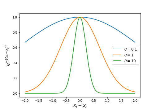
Figure 1: Changes in the correlation when varying the $\theta$ value.

II.1 Gaussian Process Regression.

In order to train a Gaussian Process Regression (GPR) model, a dataset of $n$ points $\{(x_{1},y_{1}),(x_{2},y_{2}),...,(x_{n},y_{n})\}$ is needed. Let us define the vectors $\vec{x}=(x_{1},x_{2},...,x_{n})$ and $\vec{y}=(y_{1},y_{2},...,y_{n})$. The aim of a GPR is to find the posterior probability distribution for the values of the independent variable $P(\vec{w}|\vec{y},\vec{x})$, where $\vec{w}$ is a vector of weights that defines the model. The posterior is computed by the Bayes’ Rule:

$$P(\vec{w}|\vec{y},\vec{x})=\frac{P(\vec{y}|\vec{x},\vec{w})P(\vec{w})}{P(\vec{y}|\vec{x})}.$$ (7)

Here: $P(\vec{w})$ is referred to as the prior which is a probability distribution that contains information about $\vec{w}$ before the observed data; $P(\vec{y}|\vec{x},\vec{w})$ is named the likelihood and it relates information about the prior distribution with the data; the marginal likelihood $P(\vec{y}|\vec{x})$ is a constant of normalization that guarantees the posterior is a probability ($0\leq P(\vec{w}|\vec{y},\vec{x})\leq 1$) and it is given by the integral of the numerator over all possible values of $\vec{w}$:

$$P(\vec{y}|\vec{x})=\int{P(\vec{y}|\vec{x},\vec{w})P(\vec{w})}d\vec{w}.$$ (8)

Note that Bayes’ Rule is not restricted to Gaussian distributions, however, in the context of GPR, the prior and posterior are both a GP and the data is Gaussian (each value is determined by a mean and a standard deviation). For this particular case, the prior and posterior are called conjugate distributions with respect to the likelihood function.

The GPR consists in making predictions based on the training data set (also called observables), assuming the observations are distributed around a model $f$ with an additive noise $\varepsilon$, which is assumed to be Gaussian with zero mean and variance $\sigma^{2}_{n}$:

$$\begin{matrix}\vec{y}=f(\vec{x})+\varepsilon,\\ \text{cov}{(\vec{y})}=K(\vec{x},\vec{x})+\sigma_{n}^{2}I,\end{matrix}$$ (9)

where $I$ is the identity matrix and $K(\vec{x},\vec{x})$ is the covariance matrix obtained when evaluating the kernel in the corresponding training points, that is $[K(\vec{x},\vec{x})]_{ij}=k(x_{i},x_{j})$.

Therefore, it is required to find the test outputs $\vec{f}_{*}$, which are the values of the model at the test points $\vec{x}_{*}\equiv\left({x_{1}}_{*},{x_{2}}_{*},\cdots,{x_{n}}_{*}\right)$. The posterior distribution of Eq. (7) can be derived by conditioning the prior on the training observations, such that the conditional distribution of $\vec{f}_{*}$ only contains those functions from the prior that are consistent with the data set. Using the conditioning and marginalizing properties of the Gaussian distribution on the joint distribution for $\vec{f}_{*}$ and $\vec{y}$, it can be proven Rasmussen and Williams (2006) that the mean and covariance of the predictions for the test set $\vec{x}_{*}$ is:

$$\begin{matrix}\bar{\vec{f}}_{*}=\vec{K}_{*}^{\top}(\vec{K}+\sigma_{n}^{2}\vec{I})^{-1}\vec{y}\,,\\ \text{cov}(\vec{f}_{*})=\vec{K}_{**}-\vec{K}_{*}^{\top}\left(\vec{K}+\sigma_{n}^{2}\vec{I}\right)^{-1}\vec{K}_{*}\,.\end{matrix}$$ (10)

The notation $\vec{K}=K(\vec{x},\vec{x})$, $\vec{K}_{*}=K(\vec{x},\vec{x}_{*})$ and $\vec{K}_{**}=K(\vec{x}_{*},\vec{x}_{*})$ is introduced to simplify the calculations.

II.2 Maximum likelihood estimation.

Assuming the cases in the training set are independent of each other, the probability density of the observations given a set of parameters $\vec{w}$, which is the likelihood from Eq. (7), can be expressed as a product of individual densities

$$P(\vec{y}|\vec{x},\vec{w})=\prod_{i=1}^{n}p(y_{i}|x_{i},\vec{w})\,,$$ (11)

where $n$ is the number of input training points. Therefore, using the fact that the product of Gaussian distributions is also Gaussian, the marginal likelihood from Eq. (8), in logarithmic form, becomes the log marginal likelihood

$$\footnotesize\log{P(\vec{y}|\vec{x})}=-\frac{1}{2}\vec{y}^{T}(\vec{K}+\sigma_{n}^{2}\vec{I})^{-1}\vec{y}-\frac{1}{2}\log{|\vec{K}+\sigma_{n}^{2}\vec{I}|}-\frac{n}{2}\log{2\pi}.$$ (12)

Optimal values of the parameters can be estimated by maximizing the log marginal likelihood. This training method used in GPR is known as the maximum likelihood estimation Rasmussen and Williams (2006). The maximizing can be performed by any optimizing algorithm, such as gradient descent or Markov Chain Monte Carlo.

III GP Kernel.

As seen so far, a fundamental feature of GPR which plays an important role, in the fitting of a model, is the kernel. A kernel (or covariance function) describes the covariance (correlation) of the random variables of the GP. Together with the mean function, the kernel completely defines a GP. In principle, any function that relates two points based on the distances between them can be a kernel, but it must satisfy certain conditions in order to represent a covariance function. For a function to be a valid kernel, the associated resulting matrix in Eq. (5) must be positive definite, which implies that it has to be symmetric and invertible.

The covariance function of the variables $x$ and $x^{\prime}$ is said to be stationary if it is a function only of $x-x^{\prime}$, since it is invariant under translations, and non-stationary otherwise. Moreover, if it is a function only of $|x-x^{\prime}|$ it is isotropic since it is invariant under rigid transformations.

As mentioned previously, it is necessary to choose a suitable kernel type for each particular problem. The process of creating a kernel from scratch is not always trivial, so it is usual to invoke some predefined in order to model a diversity of processes. Some of the most used kernels are Pedregosa et al. (2011):

• Radial Basis Function.

  $$k(x,x^{\prime})=\exp{\left(-\frac{d(x,x^{\prime})^{2}}{2l^{2}}\right)},$$ (13)

  where $d(x,x^{\prime})$ represents the euclidean distance between $x$ and $x^{\prime}$ and $l>0$ is known as the length parameter. Sometimes it is written in terms of a value $\theta$ that depends on the length parameter, such as in Eq. (6). It is knwon as Radial Basis Function because it depends only on the radial distance.

• Matern.

  $$\scriptsize k(x,x^{\prime})=\frac{1}{\Gamma(\nu)2^{\nu-1}}\left(\frac{\sqrt{2\nu}}{l}d(x,x^{\prime})\right)^{\nu}K_{\nu}\left(\frac{\sqrt{2\nu}}{l}d(x,x^{\prime})\right),$$ (14)

  where $K_{\nu}$ is a modified Bessel function, $\Gamma$ is the Gamma function, $l$ is the characteristic length and $\nu$ is a number that controls the smoothnes of the function. For $\nu=1/2$, the Matern kernel becomes an RBF function and some important values of $\nu$ are $\nu=1.5$ and $\nu=2.5$, which give a once and twice differentiable function, respectively.

• Exponential Sine Squared (periodic kernel).

  $$k(x,x^{\prime})=\exp{\left(-\frac{2\sin^{2}{(\pi d(x,x^{\prime})/p)}}{l^{2}}\right)},$$ (15)

  where $p>0$ is the periodicity parameter.

• Dot Product.

  $$k(x,x^{\prime})=\sigma_{0}^{2}+x\cdot x^{\prime},$$ (16)

  where $\sigma_{0}$ is a parameter that controls the inhomogeneity of the kernel.

• Rational Quadratic.

  $$k(x,x^{\prime})=\left(1+\frac{d(x,x^{\prime})^{2}}{2\alpha l^{2}}\right)^{-\alpha},$$ (17)

  where $\alpha$ is known as the scale mixture parameter.

Each of the values that can be varied within the kernel, such as $l$, $\sigma_{0}$, etc. are called hyperparameters. It is said that GPR is a non-parametric technique because the number of hyperparameters is infinite. The reader might have noticed that all kernels described above are stationary (dependent on $|x-x^{\prime}|$), except Dot Product. This dependence on distance alone makes stationary kernels more rigid, while also presenting poor predictive power when outside the scope of the used data when compared with their non-stationary counterparts. Non-stationary kernels are more flexible, which allows for a better estimate outside the scope covered by the observations. Nevertheless they are rarely used given the high number of hyperparameters to optimize, higher complexity, high computational costs and a greater risk of overfitting when compared against stationary ones Paciorek and Schervish (2003, 2006); Noack and Sethian (2022); Noack et al. (2024). In this work we will use exclusively stationary kernels and Dot Product, although we think that the idea of using non-stationary ones for cosmological observations might be worth visiting in a future work.

Since the kernel is a key feature of GPR, modifying it might produce different models. Therefore, it is necessary to establish which kernel is the best option for a particular model. In a real problem, such as those presented in Cosmology, the kind of relationship between two variables is not always previously known. In these cases, the kernel that results in the best fit after regression may be chosen from a set of default kernels.

III.1 Kernel selection through $\chi^{2}$.

A robust statistical tool, known as the $\chi^{2}$ test, could be employed to determine which model, derived from various kernels, fits best a specific dataset, thereby enhancing the regression analysis. This test evaluates the congruence between two datasets by assessing whether a significant discrepancy exists between the observed data values and the model’s predictions.

The method consists in defining the objective function $\chi^{2}$ as:

$$\chi^{2}=\sum_{i,j}\big{(}y_{i}-f(x_{i})\big{)}C_{ij}^{-1}\big{(}y_{j}-f(x_{j})\big{)},$$ (18)

where $(x_{i},y_{i})$ are the data points (or training set), $C_{ij}$ is the covariance matrix and $f(x_{i})$ are the values of the model at the independent variable of the data points. When the covariance matrix is diagonal we obtain a simplified case for the $\chi^{2}$ as:

$$\chi^{2}=\sum_{i}{\frac{[y_{i}-f(x_{i})]^{2}}{\sigma_{y_{i}}^{2}}},$$ (19)

where $\sigma_{y_{i}}^{2}$ is the variance and the $i$th element in the diagonal of $C_{ij}$. The GPR produces a model data set that can be interpreted as a function $f$ of the independent variable $x$. Given an observable $(x_{i},y_{i})$, the numerator of Eq. (19) represents the squared distance between the observable and the model for the same value of $x_{i}$. By computing this difference over all the available observations (and as such calculating the $\chi^{2}$ function) we can get an idea on how well model $f$ fits the data.

If the value of $\chi^{2}$ is obtained for models built with different kernels, the best fit will be the one that minimizes this objective function. Notice that this method is different from the maximum likelihood estimation explained in Section II.2, since it is not used to determine the hyperparameters as in the training. In this case, the models of regression have been determined previously for different kernels and tested to find the best model in terms of the covariance function.

III.2 A generic example.

In this section, regression models based on Gaussian Processes are constructed from a mock dataset exhibiting a straight-line behavior. Fortunately, nowadays there is a broad range of standard developed code and libraries that facilitate performing a Gaussian Process Regression, such as GPy GPy (2012), GPflow van der Wilk et al. (2020), GPyTorch Gardner et al. (2018), PyMC Abril-Pla1 et al. (2023), scikit-learn Pedregosa et al. (2011) and GaPP Seikel et al. (2012b). The latter two are the ones used during the course of this example and the complete step-by-step procedure can be found at the public repository Ugalde (2023). To further simplify, the construction of a GPR model consists of 3 steps: 1) specify the prior distribution via the kernel, 2) find the hyperparameters that maximize Eq. (12) and 3) evaluate predictions with Eqs. (10) using the optimal hyperparameters and observables.

We will use the function GaussianProcessRegressor(), which initializes a GP prior for regression with a specified kernel and its parameters. The method fit() returns the same GaussianProcessRegressor() object fitted to the observables using the maximum likelihood estimation. This method takes two lists as parameters that correspond to the observational data variables $\vec{x}$ and $\vec{y}$. Finally, the predict() method returns the means and standard deviations of the predictions using Eqs. (10).

In the first of our examples of regression, the variances $\sigma_{y_{i}}^{2}$ or noises of the observational data are ignored. This approach assumes that the data measurements are exact, therefore implying there are no uncertainties or error bars associated to them.

A mock data set scattered around a linear equation $Y=mX+b$ with $m=3$ and $b=-4$ is created by adding a random value between $-15$ and $15$ to $10$ evaluations of the equation at different values of $X\in[0,10]$. The aim of the GPR is to reproduce the graph of the line that originated the set.

In this case, the $\chi^{2}$ test cannot be used to find an optimal kernel, since Eq. (18) is undefined, thus an alternative method to determine the kernel must be used. The predictions of the model using a specific kernel at different values of $X$ will be compared via the sum of squared euclidean distances to the points of the original linear relationship at the corresponding $X$-values scaled by the number of data points, $n$. The result is called Mean Squared Error (MSE) and can be written as:

$${\rm MSE}=\frac{1}{n}\sum_{i}{[y_{i}-f(x_{i})]^{2}}.$$ (20)

The regression model that minimizes the MSE is the one that most resembles the desired line. At this point, without loss of generality, the kernel used in this GPR is the Matern (Eq. (14)).

Figure 2 shows the observational mock dataset (black points), the model predictions (blue solid line), the line from which the data was obtained (red dash) and the confidence zones (in lilac colors) that correspond to $2\sigma$ and $3\sigma$, respectively. These confidence intervals will be used for all the regression models along this work.

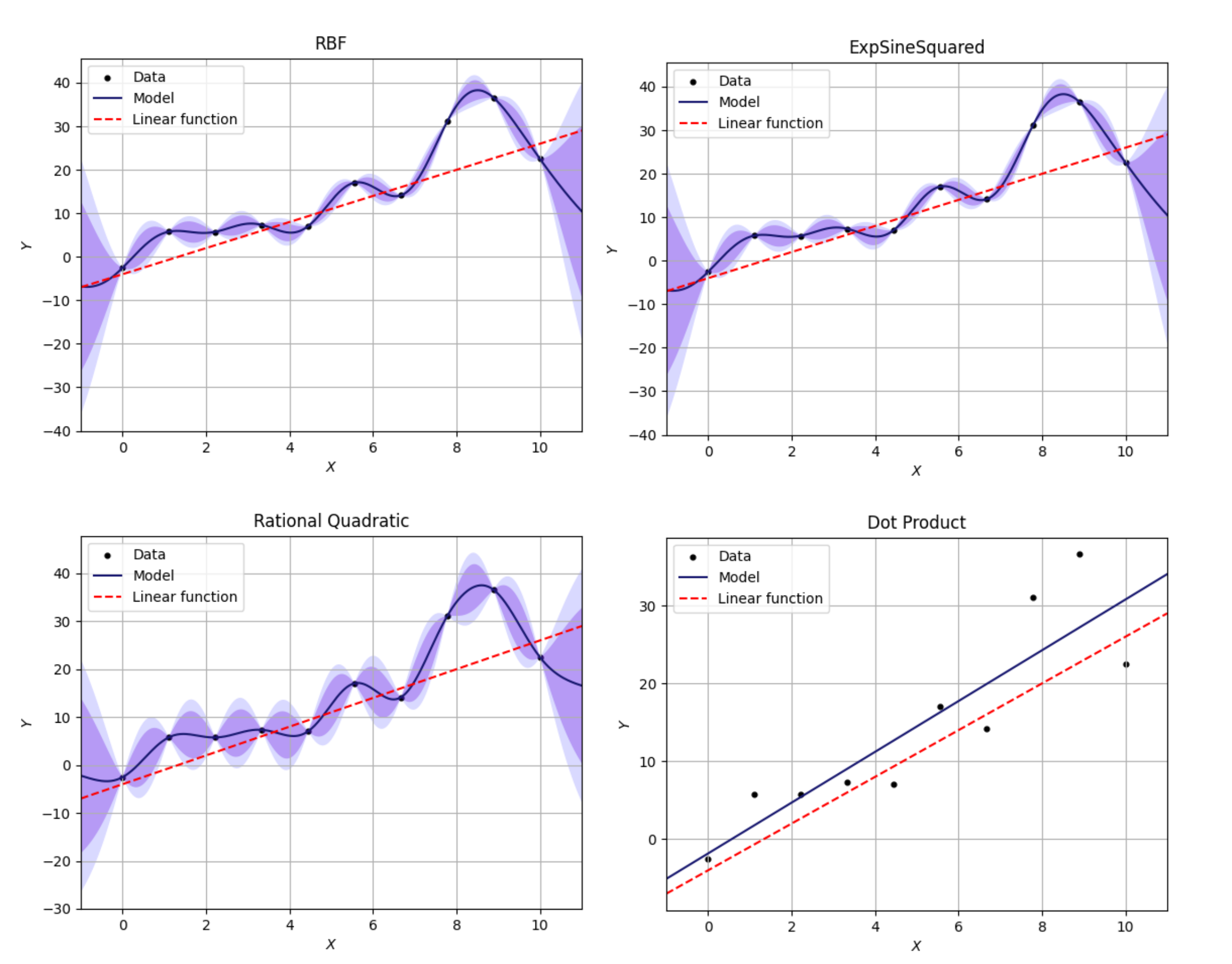
Figure 15: Models obtained from different kernels for the same linear regression with null variances.

The kernel used for this example (Figure 2) was the Matern, as we tested different ones and the results achieved are quite similar, however, as can be seen in Figure 3, this is not the kernel that minimizes the MSE, which corresponds to the Dot Product kernel. The linear regression models for each kernel are shown in Figure 15. Notice that the Dot Product kernel produces a linear regression model, so it is usually the best choice when fitting a straight line. In contrast, for the rest of the kernels, the uncertainty reduces to zero when the model is evaluated at the observations. This can be interpreted as the model overfitting the data, which is expected given that the mock data presents no variances Ó Colgáin and Sheikh-Jabbari (2021). To mitigate overfitting, one approach is to introduce an additional hyperparameter, $\sigma_{n}$, for noise modeling. This hyperparameter accounts for the observational noise, preventing the model from fitting the data too precisely. However, adding $\sigma_{n}$ increases the model complexity, requiring careful tuning to balance the bias and variance Rasmussen and Williams (2006).

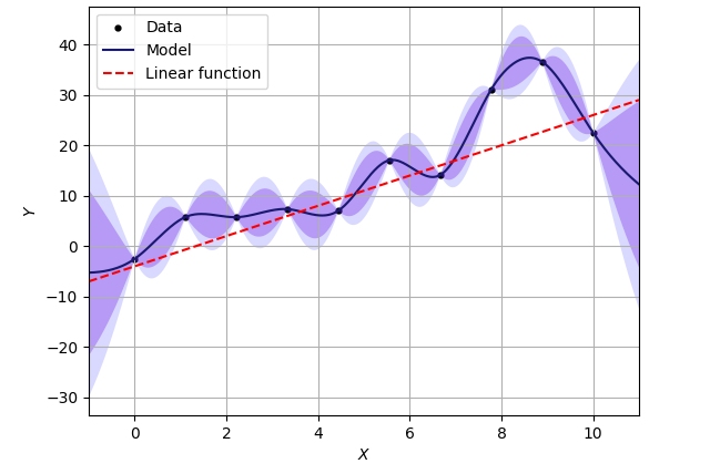
Figure 2: Linear model with null variances in the data. A Matern kernel was used for the reconstruction. It is evident that there is an overestimation of the confidence zone because our data lacks errors.

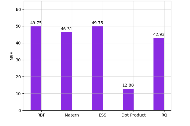
Figure 3: Comparison of Mean Squared Errors for models with different kernels.

On the other hand, when the observables do have uncertainties (which is the case that most closely resembles real data), the variances must be added to the diagonal of the kernel matrix as shown in Eq. (9). If these uncertainties come in the form of a non-diagonal covariance matrix then it is also added to the kernel so that:

$$\text{cov}{(\vec{y})}=\vec{K}+\vec{C},$$ (21)

with $\vec{C}$ being the covariance matrix of the data. The GaussianProcessRegressor() function is able to get as an input an array alpha whose size is equal to the number of data that corresponds to the variances associated with each observation. The outcome of this approach, illustrated in Figure 4, demonstrates that the prediction more closely resembles a straight line, especially when compared to the scenario with a mock dataset with null variances.

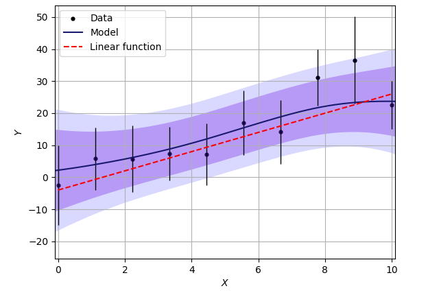
Figure 4: Linear model with variances in the data. An almost linear behavior is observed as we no longer have overfitting.

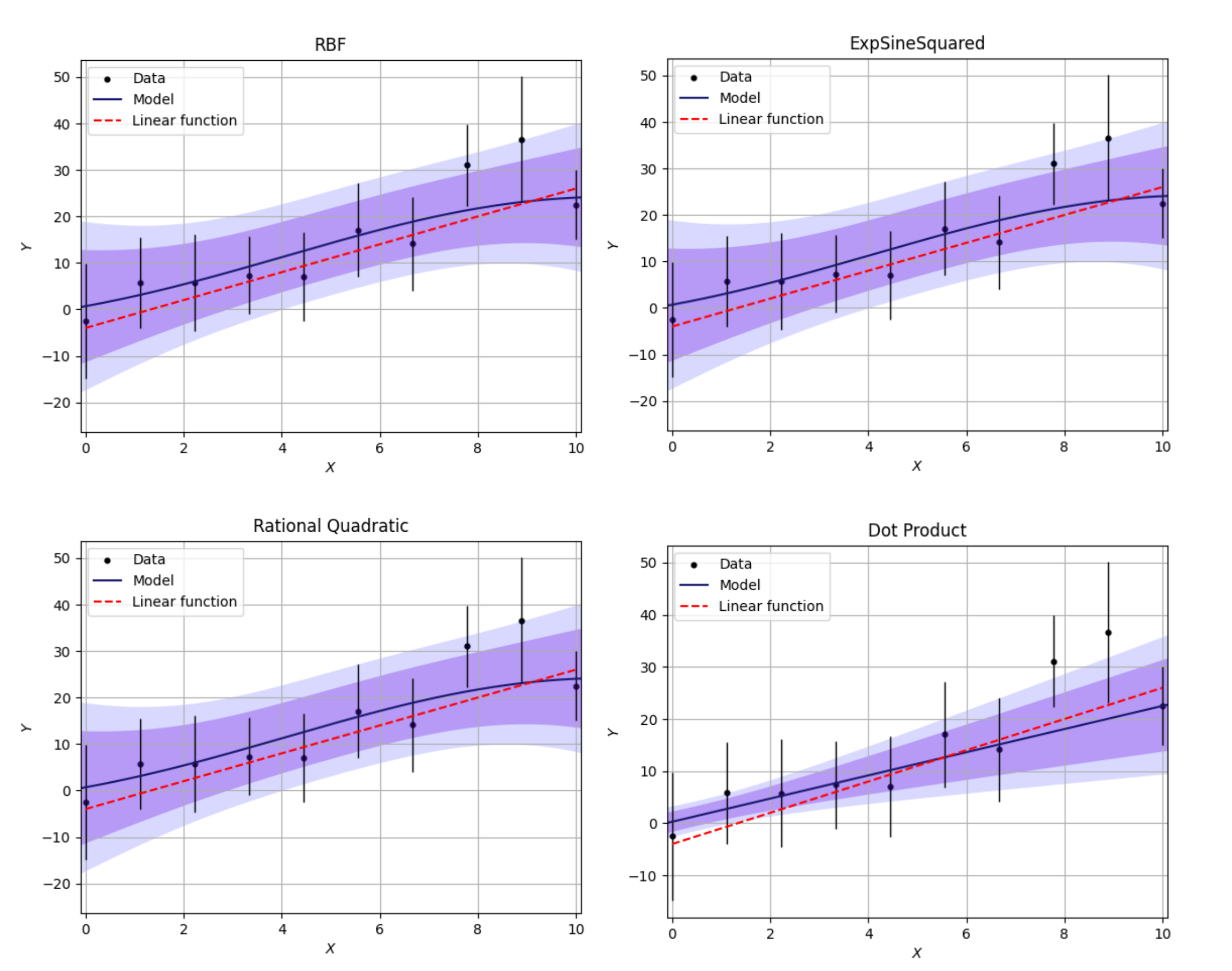
Figure 16: Linear regression models from different kernels with non-zero variances.

In this scenario, a $\chi^{2}$ test can be employed to determine the kernel that generates the optimal model. This involves creating a model for each kernel test, computing the $\chi^{2}$ value for each model, and selecting the one with the lowest $\chi^{2}$. In Figure 5 we plot the results of this test and by analyzing it it can be concluded that the model that yields the best fit to our data is the one utilizing a Matern kernel, as it produces the lowest value of the objective function. It is crucial to note that the model with the lowest $\chi^{2}$ is not necessarily the best one, as excessively minimizing $\chi^{2}$ can lead to overfitting. The linear regression models for each kernel are shown in Figure 16

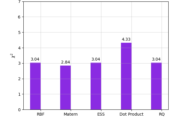
Figure 5: Values of $\chi^{2}$ for linear models with different kernels.

III.3 Derivatives of a GP.

The RBF kernel (Eq. (13)) is infinitely differentiable and the derivative of a GP is also a GP, which allows to reconstruct the derivatives of a function from data. In order to reconstruct the derivative, not only the covariance between the observational data is required but also the covariance between the function and its derivative and among the derivatives of the reconstruction. All of them can be calculated from the derivative of the kernel function as described in Seikel et al. (2012c).

As in Section II.1, it can be proven that the mean and covariance of the prediction for the first derivative of this function at test points $\vec{x}_{*}\equiv\left({x_{1}}_{*},{x_{2}}_{*},\cdots,{x_{n}}_{*}\right)$ using a differentiable kernel $k(x_{i},x_{j})$ are:

$$\begin{matrix}\bar{\vec{f}^{\prime}_{*}}=\vec{K}_{*}^{\prime\top}(\vec{K}+\sigma_{n}^{2}\vec{I})^{-1}\vec{y}\,,\\ \text{cov}(\vec{f}^{\prime}_{*})=\vec{K}^{\prime\prime}_{**}-\vec{K}_{*}^{\prime\top}\left(\vec{K}+\sigma_{n}^{2}\vec{I}\right)^{-1}\vec{K}_{*}^{\prime}\,.\end{matrix}$$ (22)

Here, $\vec{K}_{*}^{\prime}=K^{\prime}(\vec{x},\vec{x}_{*})=\frac{\partial k(x_{i},{x_{j}}_{*})}{\partial{x_{j}}_{*}}$ and $\vec{K}^{\prime\prime}_{**}=K^{\prime\prime}(\vec{x}_{*},\vec{x}_{*})=\frac{\partial^{2}k({x_{i}}_{*},{x_{j}}_{*})}{\partial{x_{i}}_{*}\partial{x_{j}}_{*}}$ are introduced to simplify the notation.

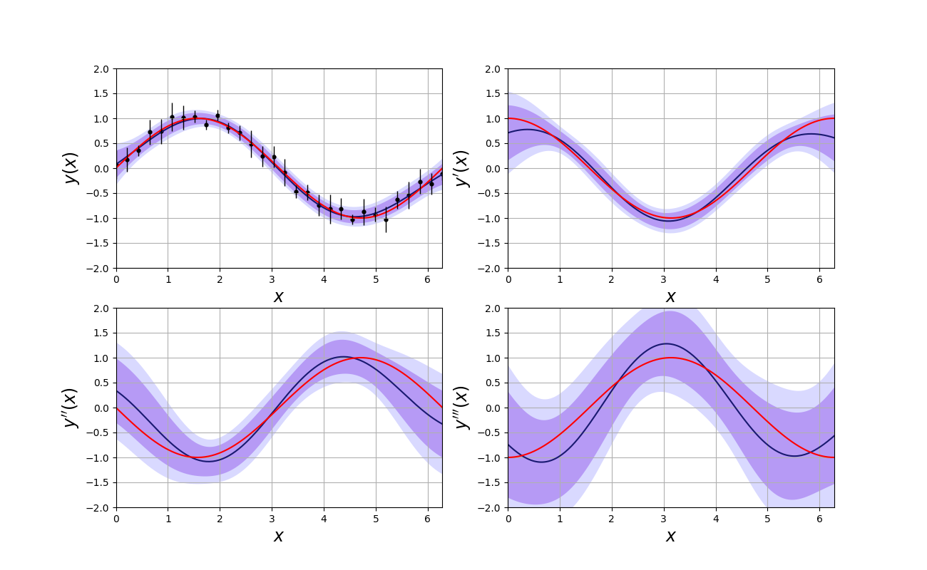
Figure 6: Reconstruction of an example test function $f(x)=\sin{x}$ and its derivatives on $[0,2\pi]$ from a mock data set. The red lines represent the analytical function or derivative and the blue lines are the predictions.

As can be inferred from these equations, the derivative of the kernel must exist in order to compute the predictions of a derivative using GPR. Therefore, an infinitely differentiable covariance function is useful when reconstructing a derivative from data, this is why an RBF kernel (Eq. (13)) is preferred among others in this type of problems. If an RBF kernel is used, the procedure can be generalized to any derivative of the model and, in particular, the package GaPP Seikel et al. (2012b) allows to compute up to the third derivative of a function quickly.

In order to verify the reliability of the code, a mock data set of values scattered around a sinusoidal function $y(x)=\sin(x)$ was created by adding a random value between $-0.15$ and $0.15$ for different values of $x$. Then the standard deviation (the error bar) of each data point was emulated by a random number between $0.1$ and $0.3$. The reconstructions of the function and its derivatives are shown in Figure 6. The red lines represent the analytical function (the sine function or its derivatives as appropriate) and the blue lines are the regression models. The confidence zones correspond to the intervals delimited by $2\sigma$ ($95\%$) and $3\sigma$ ($99\%$), where $\sigma$ are the standard deviations of the predictions. Note that the analytical function is in the $2\sigma$ interval for all the cases, which indicates that the regression is considerably accurate.

Figure 6 shows only the scatter plot of the mock data set because the observables for the derivatives do not exist. This is an advantage of the technique, since it is possible to find the $n$th-derivative of a function only from data values of such function.

IV Cosmology

Let us start by considering the Universe being homogeneous on scales larger than $150\text{ Mpc}$, which means that the distribution of its components does not depend on the position of the observer, despite the fact that at short distances the density of matter is perceived as random. Likewise, let us also assume the Universe is isotropic, which implies that its properties are the same regardless of the direction from which they are observed. The assumption of these two characteristics (homogeneity and isotropy at large scales) is known as the Cosmological Principle and it has been adopted to set restrictions on a great variety of alternative cosmological theories.

It is firmly established by observations that our Universe expands Sharov and Novikov (1993). The standard Big Bang model proposes that the Universe emerged about $15$ billion years ago and it has been expanding and cooling since then. Measurements using Type IA supernovae as standard candles have proven that the expansion of the Universe is also accelerating Perlmutter et al. (1999); Riess et al. (1998) and such acceleration is only possible if a substantial fraction of the total energy density is a kind of energy with a negative pressure Copeland et al. (2006). This energy component is referred to as Dark Energy (DE) given its unknown nature and origin. Furthermore, along with DE, another key component, known as Dark Matter (DM), is necessary to explain observations regarding structure formation. Given the enigmatic nature of both DE and DM, predicting the Universe’s long-term future remains an elusive task. Consequently, DE and DM represent two of the most compelling and complex challenges in contemporary cosmology.

The expansion of the Universe is described by the Friedmann equations, obtained as solutions of the Einstein field equations for the Friedman-Lemaitre-Robertson-Walker (FLRW) metric and a perfect fluid with density $\rho$ and pressure $p$. The equations in standard form are:

$$H^{2}=\left(\frac{\dot{a}}{a}\right)^{2}=\frac{8\pi G}{3}\rho-\frac{kc^{2}}{a^{2}},$$

$$\frac{\ddot{a}}{a}=-\frac{4\pi G}{3}\left(\rho+\frac{3p}{c^{2}}\right),$$ (23)

where $a$ is known as the scale factor, which is a dimensionless function of time and is related to the size of the Universe; $\dot{a}$ and $\ddot{a}$ denote the first and second derivative of $a$ with respect to the cosmic time; $H$ is the Hubble parameter, which describes how fast the Universe is expanding; $G$ is the gravitational constant; $c\approx 3\times 10^{5}\text{ km}/\text{s}$ is the speed of light in vacuum and $k$ is the curvature parameter, which determines the shape of the Universe Mukhanov (2005).

One of the most favored models by evidence is the $\Lambda$CDM. This model proposes that the DM component of the Universe is a non-relativistic (cold) that only interacts gravitationally, while the DE is due to an unknown component represented by the cosmological constant $\Lambda$. As mentioned previously, DE is an exotic component in the energy budget of the Universe, which is theorized to be responsible for its accelerated expansion. Most cosmological models consider DE to be a perfect fluid, which means that it is incompressible and with zero viscosity. Then it follows that, for a perfect fluid, its equation of state (EoS) is characterized by a dimensionless value $w$. In the case of barotropic fluids $w$ given by the proportionality function between its pressure $p$ and energy density $\rho$:

$${p}=c^{2}w{\rho}.$$

For perfect fluids such as baryonic matter and relativistic matter (radiation) their EoS’s are $w=0$ and $w=1/3$, respectively. Understanding the behavior of the Dark Energy’s equation of state is a focal point of contemporary cosmology. It is established that the pressure exerted by DE must be negative, given its role in driving cosmic expansion instead of contraction. Furthermore, accelerated expansion is predicted to occur when the equation of state parameter falls below $-1/3$. When working with the $\Lambda$CDM model one assumes that $w=-1$ for the DE, giving its characteristic behavior of a cosmological constant.

For the standard cosmological model, taking into consideration the equations of state for every component when solving Eq. 23, the Hubble parameter obtained from the first Friedmann equation in terms of the present values of the density parameters $\Omega_{i}$ is:

$$\small{H(z)=H_{0}\sqrt{\Omega_{r,0}a^{-4}+\Omega_{m,0}a^{-3}+\Omega_{k,0}a^{-2}+\Omega_{\Lambda,0}}},\,$$ (24)

where the density parameters are $\Omega_{r,0}$ for radiation, $\Omega_{m,0}$ for the matter sector, which includes DM and baryons, $\Omega_{k,0}$ to account for the spatial curvature, $\Omega_{\Lambda,0}$ to describe the vacuum density in the form of a cosmological constant (this represents the DE component) and $H_{0}$ the Hubble parameter, known as the Hubble constant. The subscript “0” means that they are evaluated at the present time. For a spatially flat model ($\Omega_{k}=k=0$) we have $\Omega_{m}+\Omega_{r}+\Omega_{\Lambda}=1$.

In order to determine a concept of distance between two objects in the Universe, it is convenient to present some common definitions of distance measures in Cosmology Peebles (1993); Hogg (1999), these include:

1. Comoving distance: Due to the homogeneity of the Universe, it is possible to define a coordinate system that considers the expansion of the Universe. The distance between two objects in this system remains constant, so the comoving distance is defined as

$$d_{C}(z)=d_{H}\int_{0}^{z}{dz^{\prime}\frac{H_{0}}{H(z^{\prime})}},$$ (25)

where $d_{H}=\frac{c}{H_{0}}$ is the Hubble distance.

2. Transverse comoving distance: When considering the curvature intrinsic to the geometry of space-time, expressed by the parameter $\Omega_{k}$, the transversal comoving distance is defined as,

$$d_{M}=\begin{cases}\frac{d_{H}}{\sqrt{\Omega_{k}}}\sinh{\left(\frac{\sqrt{\Omega_{k}}d_{C}(z)}{d_{H}}\right)}&\text{ if }\Omega_{k}>0,\\ d_{C}(z)&\text{ if }\Omega_{k}=0,\\ \frac{d_{H}}{\sqrt{-\Omega_{k}}}\sin{\left(\frac{\sqrt{-\Omega_{k}}d_{C}(z)}{d_{H}}\right)}&\text{ if }\Omega_{k}<0,\end{cases}$$ (26)

which is equal to the comoving distance in the case of a flat space-time, i.e. for $\Omega_{k}=0$.

3. Luminosity distance: Comparing the absolute and apparent magnitudes between two objects, that is, the actual brightness emitted by an object compared to the brightness observed from Earth, the luminosity distance is defined, which is written in terms of the transverse comoving distance as:

$$d_{L}(z)=(1+z)d_{M}(z).$$ (27)

From the above equations, the normalized comoving distance is also obtained as,

$$D(z)=\frac{1}{d_{H}}\left(\frac{1}{1+z}\right)d_{L}(z).$$ (28)

In the particular case of a flat Universe, a simple expression for the derivative of the normalized comoving distance can be obtained:

$$D^{\prime}(z)=\frac{H_{0}}{H(z)}.$$ (29)

The cosmological quantities are broadly categorized into two groups - the physical (dynamical) quantities like the DE equation of state parameter $w$, vs the kinematical (cosmographical) quantities that are defined as time derivatives of the scale factor $a$, for example, the Hubble $H$, deceleration $q$ and jerk $j$ parameters. The deceleration parameter is defined as:

$$q=-\frac{\ddot{a}a}{\dot{a}^{2}},$$ (30)

which can be written in terms of the derivatives of $D(z)$ with respect to the redshift $z$, as

$$q(z)=-1-\frac{D^{\prime\prime}(z)}{D^{\prime}(z)}(1+z),$$ (31)

or, in terms of $H(z)$ and its derivative $H^{\prime}(z)$, as

$$q(z)=-1-\frac{H^{\prime}(z)}{H(z)}(1+z)\,.$$ (32)

The deceleration parameter is a measure of the acceleration of the expansion of space, and it is said to be accelerating when $q$ becomes negative Peebles (1993).

Furthermore, with DE having a time-varying dynamical equation of state $w(z)$ (ignoring the contribution from spatial curvature and radiation), we can write the Hubble parameter $H(z)$ by integrating the Friedmann equation (23) as,

$$\frac{H^{2}(z)}{H_{0}^{2}}=\Omega_{m,0}(1+z)^{3}+(1-\Omega_{m,0})e^{3\int_{0}^{z}\frac{1+w(x)}{1+x}dx}.$$ (33)

On differentiating the above equation one can arrive at this expression for the DE equation of state $w(z)$, as

$$w(z)=\frac{2(1+z)H(z)H^{\prime}(z)-3H^{2}(z)}{3H^{2}(z)-\Omega_{m,0}H_{0}^{2}(1+z)^{3}}\,.$$ (34)

As the deceleration parameter $q$ is now estimated and found to be evolving, we focus on the next higher-order derivative, the jerk parameter $j$, defined as

$$j=\frac{\dddot{a}}{aH^{3}}\,.$$ (35)

It can be rewritten as a function of redshift $z$, in terms of the Hubble parameter $H$ along with its derivatives $H^{\prime}(z)$ and $H^{\prime\prime}(z)$, as

$$j(z)=1-2(1+z)\frac{H^{\prime}}{H}+(1+z)^{2}\left(\frac{H^{\prime\prime}}{H}+\frac{H^{\prime 2}}{H^{2}}\right)\,.$$ (36)

For the $\Lambda$CDM model $j$ is exactly unity. So, any non-monotonic evolution of $j$ can help in understanding the nature of dark energy in the absence of any convincing physical theory Alam et al. (2003); Sahni et al. (2003).

Figure 7: Hubble parameter reconstruction model using a Matern kernel.

V Cosmological functions with GPR

V.1 Hubble parameter

In Cosmology, the aim is to find a mathematical description that explains the characteristics of the Universe and predicts its evolution over time. Thus determining the dependency of $H$ as a function of $z$ is one of the main topics of study in Cosmology.

For the above, the regression method with GP is a very useful tool as it allows to reconstruct the evolutionary model from certain observational data. In this case, the data will be Hubble parameter observations for different redshifts from cosmic chronometers as an alternative to the commonly used data from Type Ia Supernovae. There is a set of $31$ data points for $H(z)$ obtained by different authors, which have been gathered and used in many works, such as Gómez-Valent and Amendola (2018) and Vagnozzi et al. (2021). Using the developed code that contains variances and the Hubble parameter data, the model shown in Figure 7 is obtained.

The curve for $H(z)$ in the $\Lambda$CDM model was created from Eq. (24) and the values for the density parameters given by Planck results Akrami et al. (2018), were obtained under the assumption of a flat Universe as $\Lambda$CDM.

Various models were tested with different kernels as shown in Figure 9. The model that minimizes $\chi^{2}$ for $H(z)$ was produced by a Matern kernel with the default initial characteristic length of $l=1$ and an order of $\nu=1.5$. The optimized hyperparameter after the training is $l=4.1$.

Evaluating the model for $z=0$, a value for the Hubble constant of $H(0)=68.798\pm 6.340(1\sigma)\text{ km}\text{ Mpc}^{-1}\text{ s}^{-1}$ is obtained as can be seen at Ugalde (2023).

V.2 Dark Energy equation of state

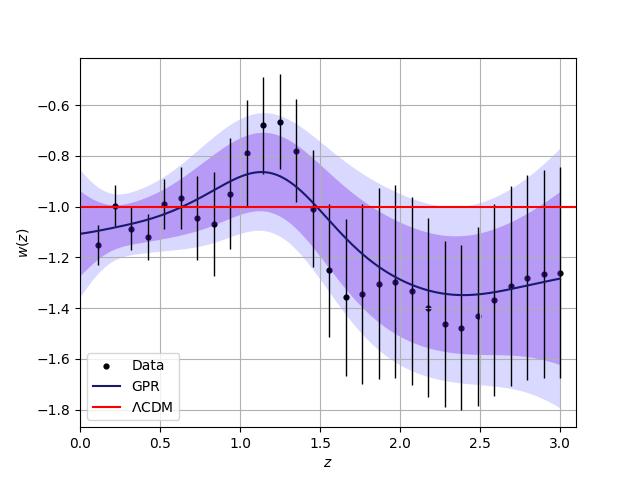
Figure 8: Reconstruction model for the dark energy equation of state.

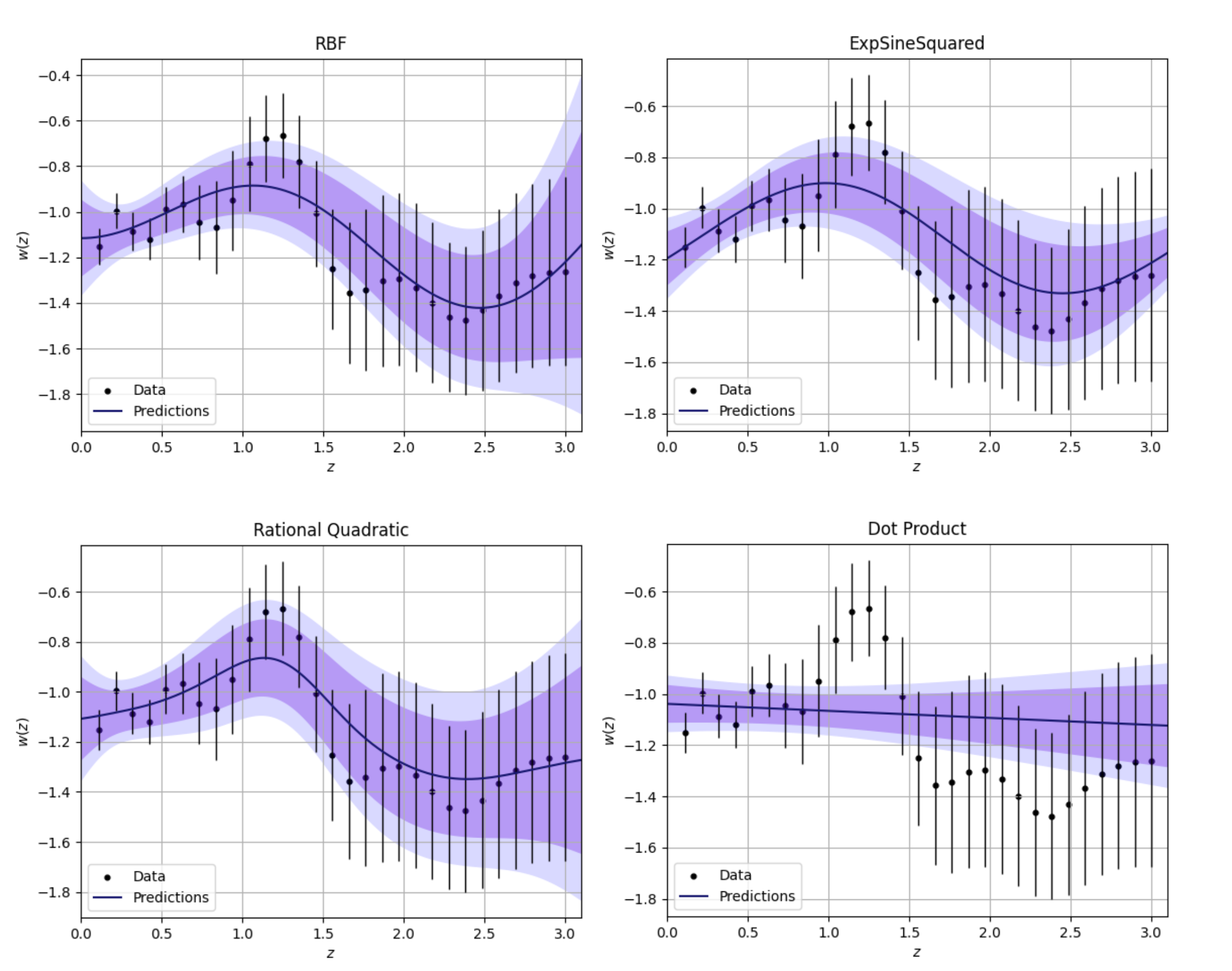
Figure 18: Regression models of Dark Energy for different kernels.

If the DE is considered as a dynamic component, then its EoS should be different from $-1$ (so as to differentiate itself from $\Lambda$CDM), or it could present a dependence on redshift as $w(z)$. As a proof of the concept and using the previously established methods, we will use a mock dataset from the dark energy equation of state as a function of $z$ to reconstruct it. As such, a non-parametric model of $w(z)$ with GPR using a RQ kernel will be obtained (Figure 8). In Figure 9, a comparison of the values of $\chi^{2}$ for models obtained using different kernels is shown and the different model can be seen in Figure 18. Note that when reconstructing $H(z)$, the RQ kernel was the best option since it returned the minimum values. As already stated earlier, the $\Lambda$CDM model EoS for DE is proposed as a constant of value $-1$, so if there are cracks in the standard model then our reconstruction should find deviations from this value. In our case, it was found that a $w=-1$ is well within 1$\sigma$ bounds of the reconstruction using GPR, which can be interpreted as weak evidence against $\Lambda$CDM.

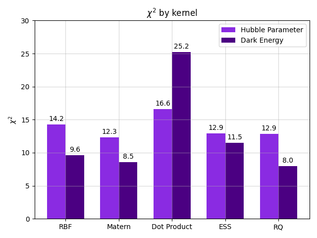
Figure 9: Comparison between the $\chi^{2}$ values for models of Hubble parameter and dark energy equation of state with different kernels

V.3 Reconstruction of the deceleration parameter

By using $H(z)$ data from cosmic chronometers, the predicted value of $H_{0}=68.798\text{ km}\text{ Mpc}^{-1}\text{ s}^{-1}$ and Eq. (29), we can obtain a derived dataset of $D^{\prime}(z)$. To obtain the variances/errors of this new dataset it is straightforward to use the approximation of a ratio distribution for uncorrelated variables. So far, the Matern kernel has presented the most suitable models (at least regarding the $\chi^{2}$ obtained), henceforth this kernel will be used for the reconstruction. The resulting GPR prediction for $D^{\prime}(z)$ from the derived dataset and a comparison with the $\Lambda$CDM values computed by combining Eq. (29) and Eq. (24) with the corresponding density parameters and the value of $H_{0}=67.32\text{ km}\text{ Mpc}^{-1}\text{ s}^{-1}$ from Planck results Akrami et al. (2018) are shown in Figure 10.

From the same dataset of $D^{\prime}(z)$ the derivative $D^{\prime\prime}(z)$ is reconstructed using the GaPP package as explained in Section III. On the other hand, Eq. (29) can be differentiated analytically and evaluated for the $\Lambda$CDM density parameters to obtain $D^{\prime\prime}(z)$. Figure 11 shows the predictions for $D^{\prime\prime}(z)$ and a comparison with $\Lambda$CDM. Finally, from Eq. (31) and the GPR predictions of $D^{\prime}(z)$ and $D^{\prime\prime}(z)$ a model of the deceleration parameter is produced as in the previous cases. The regression is compared with $\Lambda$CDM in Figure 12. We see again some agreement between our reconstruction and the standard model, although an important thing to note is that there is a region where $\Lambda$CDM remains outside the 1$\sigma$ contour and it is really close to being outside the 2$\sigma$ one. This could indicate some actual evidence in favor of our reconstruction or at least highlight a tension existing within $\Lambda$CDM. Similar discrepancies have been noted in previous studies, where deviations from $\Lambda$CDM behavior were observed in various cosmological datasets Lin et al. (2019); Gómez-Valent (2019); Haridasu et al. (2018); Mukherjee and Banerjee (2022b). These findings suggest potential new physics beyond the standard cosmological model or the need for refined cosmological parameters which calls for further investigation.

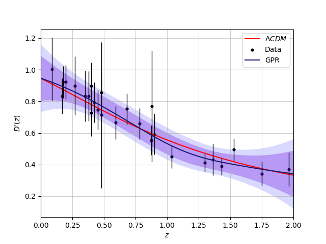
Figure 10: Reconstruction of the first derivative of the normalized comoving distance.

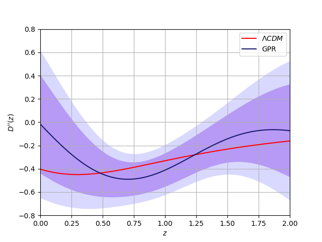
Figure 11: Reconstruction of the second derivative of the normalized comoving distance.

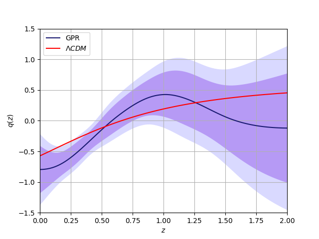
Figure 12: Reconstruction of the deceleration parameter.

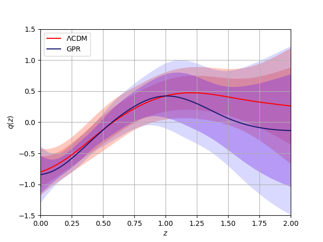
Figure 13: Comparison between the reconstruction of $q(z)$ and $\Lambda$CDM model using a mock data set.

V.4 Deceleration parameter reconstruction with a mock data set from $\Lambda$CDM

If the observables are indeed produced by the $\Lambda$CDM model (that is to say that the standard model is the “real” one), a regression using artificial data that was produced by the $\Lambda$CDM model should be quite similar to the model obtained from the “real” data. To verify this, we produced a mock dataset of $H(z)$ around the values obtained by evaluating Eq. (24) for the density parameters given by $\Lambda$CDM cosmology from Planck results Akrami et al. (2018). Then, the whole procedure to obtain $q(z)$ was repeated but this time using the mock dataset so that a comparison with the previous reconstruction could be made. The result and comparison is shown in Figure 13. As expected, the mock data set regression model is into the $2\sigma$ confidence level of the reconstruction from the observations. This indicates that, even if the standard model does not reproduce the observables exactly or does it with some caveats, it can emulate the general observed behavior pretty well.

V.5 Reconstruction of the jerk parameter

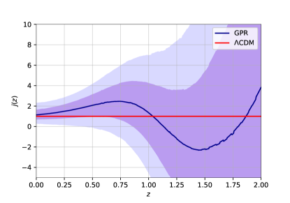
Figure 14: Comparison between the reconstruction of $j(z)$ and $\Lambda$CDM model.

From the same $D^{\prime}(z)$ dataset, derived in Section V.3, one can further reconstruct the third derivative $D^{\prime\prime\prime}(z)$ along with the second derivative $D^{\prime\prime}(z)$ employing the GaPP package as explained in Section III. With these reconstructed functions, the evolution for the cosmological jerk parameter can be obtained from Eq. (36), as a function of the redshift $z$. This regression is compared with the $\Lambda$CDM case in Figure 14. We find that our reconstruction includes the $\Lambda$CDM model (i.e., $j=1$) within the $1\sigma$ confidence level. The mean of the reconstructed function clearly indicates that $j$ has a non-monotonic evolution, which is in agreement with the previous findings Mukherjee and Banerjee (2021b).

V.6 Using GPR as an interpolation in a Model-Independent way

Throughout this work, we have demonstrated how a GPR can be utilized in a non-parametric manner to study cosmological quantities. However, there is an alternative approach to leverage the properties of a GPR which we would like to mention. This method also employs a Gaussian Process but in a model-independent manner, as it involves inferring parameter values using datasets and Bayesian statistics. By doing so, we can directly compare our model-independent reconstruction against the standard model using Bayesian evidence and maximum log-likelihood.

The GPR in this approach is done over “nodes”. These nodes can vary in height (their ordinate position), and these “variable heights” work as the new parameters of the reconstruction Alberto Vazquez et al. (2012); Hee et al. (2017). For $n$ nodes we have $n$ variable heights and, as such, $n$ new parameters which need to be inferred. This method has been used before with the equation of state of Dark Energy Gerardi et al. (2019), the interaction kernel of an IDE (interacting Dark Energy) model Escamilla et al. (2023), and the cosmic reionization history Krishak and Hazra (2021); Mukherjee et al. (2024c).

VI Discussion and Conclusions

Although Gaussian Process Regression (GPR) does not yield an explicit form of the relationship between variables, it remains a robust method for making predictions given a particular set of observables. It reconstructs functions effectively without needing prior assumptions about their behavior, leveraging libraries like GaPP to predict higher derivatives, such as $D^{\prime\prime}(z)$ and $H^{\prime}(z)$, which is particularly valuable in cosmological analyses.

GPR has been extensively applied in cosmology, spanning from reconstructing the dark energy equation of state $w(z)$ to cosmographical studies. This flexibility allows GPR to adapt to diverse datasets, making it a powerful tool for probing dark energy and other cosmological phenomena. In gravitational wave cosmology, GPR has been instrumental in reconstructing the luminosity distance from simulated data, enabling non-parametric inference of the Hubble parameter and forecasting deviations from the standard $\Lambda$CDM model. Additionally, GPR has been employed in large-scale structure studies, such as reconstructing the growth rate of cosmic structures $f\sigma_{8}(z)$ from redshift space distortions. These applications highlight GPR’s versatility in handling diverse cosmological datasets and addressing critical questions within the cosmological context.

However, GPR is constrained by the range of observed data, limiting its predictive accuracy outside this interval. Furthermore, uncertainties in derivative function reconstructions increase beyond the data range, which can impact the reliability of extrapolations. The choice of kernel function in GPR is pivotal, influencing prediction means and covariances significantly. Despite methods like cross-validation and Bayesian model selection to aid kernel selection, the optimal choice remains non-trivial, affecting the quality of reconstructions.

Comparing GPR with other parametric and non-parametric methods, principal component analysis Liu et al. (2019) (PCA), logarithmic parametrization Mamon and Das (2017), rational parametrization Gadbail et al. (2022), Bayesian methods Bing and Li-Xin (2020), reveals trade-offs between flexibility and interpretability. While PCA simplifies data dimensionality effectively, it may overlook intricate data complexities that GPR can capture. Bayesian methods provide comprehensive probabilistic frameworks but often require detailed prior information and intensive computational resources.

In summary, Gaussian Processes offer a powerful and flexible tool for cosmological analyses, enabling model-independent reconstructions and effective uncertainty handling. Despite computational challenges and kernel sensitivity, their widespread application in cosmology demonstrates their potential to provide nuanced insights into the evolutionary history of our Universe.

Appendix

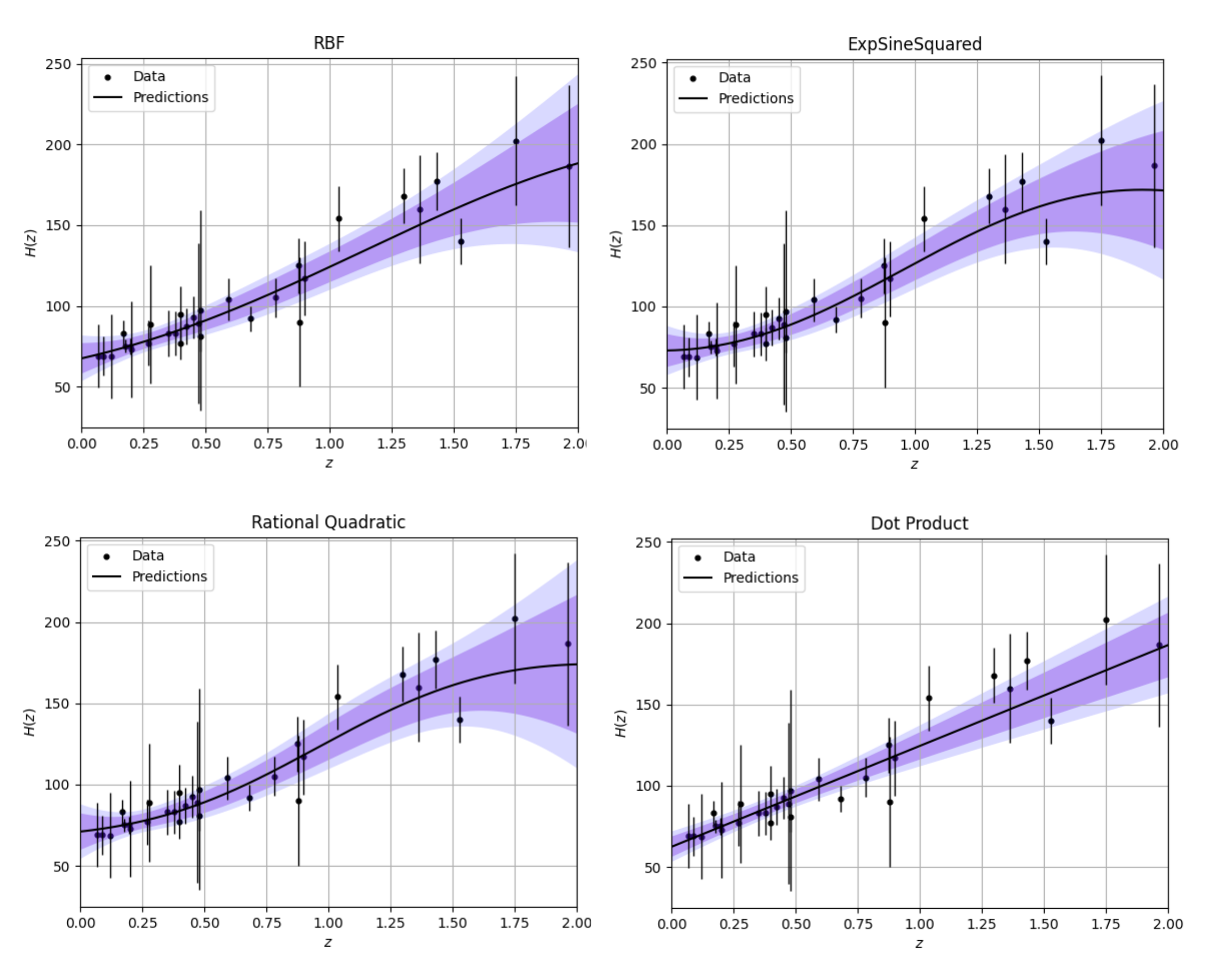
Figure 17: Regression models of Hubble Parameter for different kernels.

References

- Boggess et al. (1992) N. W. Boggess, J. C. Mather, R. Weiss, C. L. Bennett, E. a. Cheng, E. Dwek, S. Gulkis, M. G. Hauser, M. A. Janssen, T. Kelsall, et al., Astrophysical Journal, Part 1 (ISSN 0004-637X), vol. 397, no. 2, p. 420-429. 397, 420 (1992).
- Akrami et al. (2018) Y. Akrami et al., Constraints on inflation (2018).
- York et al. (2000) D. G. York, J. Adelman, J. E. Anderson Jr, S. F. Anderson, J. Annis, N. A. Bahcall, J. Bakken, R. Barkhouser, S. Bastian, E. Berman, et al., The Astronomical Journal 120, 1579 (2000).
- Astier et al. (2006) P. Astier, J. Guy, N. Regnault, R. Pain, E. Aubourg, D. Balam, S. Basa, R. Carlberg, S. Fabbro, D. Fouchez, et al., Astronomy & Astrophysics 447, 31 (2006).
- Levi et al. (2019) M. E. Levi, L. E. Allen, A. Raichoor, C. Baltay, S. BenZvi, F. Beutler, A. Bolton, F. J. Castander, C.-H. Chuang, A. Cooper, et al., arXiv preprint arXiv:1907.10688 (2019).
- Gardner et al. (2023) J. P. Gardner, J. C. Mather, R. Abbott, J. S. Abell, M. Abernathy, F. E. Abney, J. G. Abraham, R. Abraham, Y. M. Abul-Huda, S. Acton, et al., Publications of the Astronomical Society of the Pacific 135, 068001 (2023).
- Laureijs et al. (2011) R. Laureijs, J. Amiaux, S. Arduini, J.-L. Augueres, J. Brinchmann, R. Cole, M. Cropper, C. Dabin, L. Duvet, A. Ealet, et al., arXiv preprint arXiv:1110.3193 (2011).
- Chollet (2017) F. Chollet, Deep Learning with Python (Manning, 2017).
- Theobald (2017) O. Theobald, Machine Learning for Absolute Beginners: A Plain English Introduction, Ai, Data Science, Python & Statistics for Beginners (Scatterplot Press, 2017).
- Sarker (2021) I. H. Sarker, SN computer science 2, 160 (2021).
- Ray (2019) S. Ray, in 2019 International conference on machine learning, big data, cloud and parallel computing (COMITCon) (IEEE, 2019) pp. 35–39.
- Qiu et al. (2016) J. Qiu, Q. Wu, G. Ding, Y. Xu, and S. Feng, EURASIP Journal on Advances in Signal Processing 2016, 1 (2016).
- Mahesh (2020) B. Mahesh, International Journal of Science and Research (IJSR).[Internet] 9, 381 (2020).
- Dhall et al. (2020) D. Dhall, R. Kaur, and M. Juneja, Proceedings of ICRIC 2019: Recent innovations in computing , 47 (2020).
- Sewell (2023) M. Sewell, “Financial applications of neural networks,” <http://machine-learning.martinsewell.com/ann/finance.html> (2023).
- Abhishek et al. (2012) K. Abhishek, M. Singh, S. Ghosh, and A. Anand, Procedia Technology 4, 311 (2012), 2nd International Conference on Computer, Communication, Control and Information Technology( C3IT-2012) on February 25 - 26, 2012.
- Albers et al. (2019) J. Albers, C. Fidler, J. Lesgourgues, N. Schöneberg, and J. Torrado, Journal of Cosmology and Astroparticle Physics 2019, 028 (2019).
- Günther et al. (2022) S. Günther, J. Lesgourgues, G. Samaras, N. Schöneberg, F. Stadtmann, C. Fidler, and J. Torrado, Journal of Cosmology and Astroparticle Physics 2022, 035 (2022).
- Chantada et al. (2022) A. T. Chantada, S. J. Landau, P. Protopapas, C. G. Scóccola, and C. Garraffo, arXiv preprint arXiv:2205.02945 (2022).
- Chantada et al. (2023) A. T. Chantada, S. J. Landau, P. Protopapas, C. G. Scóccola, and C. Garraffo, arXiv preprint arXiv:2311.15955 (2023).
- Gómez-Vargas et al. (2023a) I. Gómez-Vargas, R. M. Esquivel, R. García-Salcedo, and J. A. Vázquez, Eur. Phys. J. C 83, 304 (2023a), arXiv:2104.00595 [astro-ph.CO] .
- Mukherjee et al. (2022) P. Mukherjee, J. Levi Said, and J. Mifsud, JCAP 12, 029 (2022), arXiv:2209.01113 [astro-ph.CO] .
- Garcia-Arroyo et al. (2024) G. Garcia-Arroyo, I. Gómez-Vargas, and J. A. Vázquez, (2024), arXiv:2404.05833 [astro-ph.GA] .
- Dialektopoulos et al. (2024) K. F. Dialektopoulos, P. Mukherjee, J. Levi Said, and J. Mifsud, Phys. Dark Univ. 43, 101383 (2024), arXiv:2305.15500 [gr-qc] .
- Mukherjee et al. (2024a) P. Mukherjee, K. F. Dialektopoulos, J. Levi Said, and J. Mifsud, (2024a), arXiv:2402.10502 [astro-ph.CO] .
- Shah et al. (2024) R. Shah, S. Saha, P. Mukherjee, U. Garain, and S. Pal, (2024), arXiv:2401.17029 [astro-ph.CO] .
- Agarwal et al. (2012) S. Agarwal, F. B. Abdalla, H. A. Feldman, O. Lahav, and S. A. Thomas, Mon. Not. Roy. Astron. Soc. 424, 1409 (2012), arXiv:1203.1695 [astro-ph.CO] .
- Agarwal et al. (2014) S. Agarwal, F. B. Abdalla, H. A. Feldman, O. Lahav, and S. A. Thomas, Mon. Not. Roy. Astron. Soc. 439, 2102 (2014), arXiv:1312.2101 [astro-ph.CO] .
- Costanza et al. (2024) B. Costanza, C. G. Scóccola, and M. Zaldarriaga, JCAP 04, 041 (2024), arXiv:2312.09943 [astro-ph.CO] .
- Gómez-Vargas and Vázquez (2024) I. Gómez-Vargas and J. A. Vázquez, (2024), arXiv:2405.03293 [astro-ph.IM] .
- Nygaard et al. (2023) A. Nygaard, E. B. Holm, S. Hannestad, and T. Tram, JCAP 05, 025 (2023), arXiv:2205.15726 [astro-ph.IM] .
- Sikder et al. (2023) S. Sikder, R. Barkana, I. Reis, and A. Fialkov, Mon. Not. Roy. Astron. Soc. 527, 9977 (2023), arXiv:2201.08205 [astro-ph.CO] .
- Jense et al. (2024) H. T. Jense, I. Harrison, E. Calabrese, A. Spurio Mancini, B. Bolliet, J. Dunkley, and J. C. Hill, (2024), arXiv:2405.07903 [astro-ph.CO] .
- Gómez-Vargas et al. (2023b) I. Gómez-Vargas, J. B. Andrade, and J. A. Vázquez, Phys. Rev. D 107, 043509 (2023b), arXiv:2209.02685 [astro-ph.IM] .
- Olvera et al. (2022) J. d. D. R. Olvera, I. Gómez-Vargas, and J. A. Vázquez, Universe 8, 120 (2022), arXiv:2112.12645 [astro-ph.CO] .
- Liu and Yang (2022) Y. Liu and S. Yang, Journal of Mathematics 2022 (2022), 10.1155/2022/6469054.
- Podgorelec et al. (2002) V. Podgorelec, P. Kokol, B. Stiglic, and I. Rozman, Journal of medical systems (2002).
- Pedregosa et al. (2011) F. Pedregosa, G. Varoquaux, A. Gramfort, V. Michel, B. Thirion, O. Grisel, M. Blondel, P. Prettenhofer, R. Weiss, V. Dubourg, J. Vanderplas, A. Passos, D. Cournapeau, M. Brucher, M. Perrot, and E. Duchesnay, Journal of Machine Learning Research 12, 2825 (2011).
- Shah et al. (2023) N. Shah, A. M. Knee, J. McIver, and D. C. Stenning, Classical and Quantum Gravity 40, 235008 (2023).
- Baker et al. (2015) P. T. Baker, S. Caudill, K. A. Hodge, D. Talukder, C. Capano, and N. J. Cornish, Physical Review D 91, 062004 (2015).
- Mucesh et al. (2021) S. Mucesh, W. G. Hartley, A. Palmese, O. Lahav, L. Whiteway, A. Bluck, A. Alarcon, A. Amon, K. Bechtol, G. Bernstein, et al., Monthly Notices of the Royal Astronomical Society 502, 2770 (2021).
- Conceição et al. (2024) M. Conceição, A. Krone-Martins, A. da Silva, and Á. Moliné, Astronomy & Astrophysics 681, A123 (2024).
- Chacón et al. (2022) J. Chacón, J. A. Vázquez, and E. Almaraz, Astron. Comput. 38, 100527 (2022), arXiv:2106.06587 [astro-ph.CO] .
- Chacón et al. (2023) J. Chacón, I. Gómez-Vargas, R. M. Méndez, and J. A. Vázquez, Phys. Rev. D 107, 123515 (2023), arXiv:2303.09098 [astro-ph.CO] .
- Ji (2021) S. Ji, “knn_recommender_system,” <https://github.com/jisilvia/kNN_Recommender_ System> (2021).
- Banerjee and Abel (2021) A. Banerjee and T. Abel, Monthly Notices of the Royal Astronomical Society 500, 5479 (2021).
- Banerjee et al. (2022) A. Banerjee, N. Kokron, and T. Abel, Monthly Notices of the Royal Astronomical Society 511, 2765 (2022).
- Yuan et al. (2023) S. Yuan, A. Zamora, and T. Abel, Monthly Notices of the Royal Astronomical Society 522, 3935 (2023).
- Wang et al. (2022) Y. Wang, A. Banerjee, and T. Abel, Monthly Notices of the Royal Astronomical Society 514, 3828 (2022).
- Nair et al. (2015) R. Nair, S. Jhingan, and D. Jain, Phys. Lett. B 745, 64 (2015), arXiv:1501.00796 [astro-ph.CO] .
- Rana et al. (2017) A. Rana, D. Jain, S. Mahajan, A. Mukherjee, and R. F. L. Holanda, JCAP 07, 010 (2017), arXiv:1705.04549 [astro-ph.CO] .
- Mukherjee and Mukherjee (2021) P. Mukherjee and A. Mukherjee, Mon. Not. Roy. Astron. Soc. 504, 3938 (2021), arXiv:2104.06066 [astro-ph.CO] .
- Mukherjee et al. (2023) P. Mukherjee, G. Rodrigues, and C. Bengaly, arXiv:2302.00867 (2023), 10.48550/arXiv.2302.00867, arXiv:2302.00867 [astro-ph.CO] .
- Shafieloo et al. (2012a) A. Shafieloo, A. G. Kim, and E. V. Linder, Phys. Rev. D 85, 123530 (2012a).
- Mukherjee and Banerjee (2021a) P. Mukherjee and N. Banerjee, Eur. Phys. J. C 81, 36 (2021a), arXiv:2007.10124 [astro-ph.CO] .
- Jesus et al. (2022) J. F. Jesus, D. Benndorf, S. H. Pereira, and A. A. Escobal, arXiv:2212.12346 (2022), 10.48550/arXiv.2212.12346, arXiv:2212.12346 [astro-ph.CO] .
- Shafieloo et al. (2012b) A. Shafieloo, A. G. Kim, and E. V. Linder, Physical Review D (2012b).
- Mukherjee and Sen (2024) P. Mukherjee and A. A. Sen, (2024), arXiv:2405.19178 [astro-ph.CO] .
- Mukherjee et al. (2024b) P. Mukherjee, R. Shah, A. Bhaumik, and S. Pal, Astrophys. J. 960, 61 (2024b), arXiv:2303.05169 [astro-ph.CO] .
- Holsclaw et al. (2011) T. Holsclaw, U. Alam, B. Sanso, H. Lee, K. Heitmann, S. Habib, and D. Higdon, Phys. Rev. D 84, 083501 (2011).
- Seikel et al. (2012a) M. Seikel, C. Clarkson, and M. Smith, JCAP 06, 036 (2012a).
- Zhang and Li (2018) M.-J. Zhang and H. Li, Eur. Phys. J. C 78, 460 (2018), arXiv:1806.02981 [astro-ph.CO] .
- Yang and Gong (2021) Y. Yang and Y. Gong, Mon. Not. Roy. Astron. Soc. 504, 3092 (2021), arXiv:2007.05714 [astro-ph.CO] .
- Dhawan et al. (2021) S. Dhawan, J. Alsing, and S. Vagnozzi, Mon. Not. Roy. Astron. Soc. 506, L1 (2021), arXiv:2104.02485 [astro-ph.CO] .
- Mukherjee and Banerjee (2022a) P. Mukherjee and N. Banerjee, Phys. Rev. D 105, 063516 (2022a), arXiv:2202.07886 [astro-ph.CO] .
- Yang et al. (2015) T. Yang, Z.-K. Guo, and R.-G. Cai, Phys. Rev. D 91, 123533 (2015), arXiv:1505.04443 [astro-ph.CO] .
- Mukherjee and Banerjee (2021b) P. Mukherjee and N. Banerjee, Phys. Rev. D 103, 123530 (2021b).
- Cai et al. (2017) R.-G. Cai, N. Tamanini, and T. Yang, JCAP 05, 031 (2017).
- Bonilla et al. (2022) A. Bonilla, S. Kumar, R. C. Nunes, and S. Pan, Mon. Not. Roy. Astron. Soc. 512, 4231 (2022), arXiv:2102.06149 [astro-ph.CO] .
- Escamilla et al. (2023) L. A. Escamilla, O. Akarsu, E. Di Valentino, and J. A. Vazquez, JCAP 11, 051 (2023), arXiv:2305.16290 [astro-ph.CO] .
- Zhou et al. (2019) L. Zhou, X. Fu, Z. Peng, and J. Chen, Phys. Rev. D 100, 123539 (2019).
- Belgacem et al. (2020) E. Belgacem, S. Foffa, M. Maggiore, and T. Yang, Phys. Rev. D 101, 063505 (2020).
- Yang (2021) T. Yang, JCAP 05, 044 (2021).
- Levi Said et al. (2021) J. Levi Said, J. Mifsud, J. Sultana, and K. Z. Adami, JCAP 06, 015 (2021), arXiv:2103.05021 [astro-ph.CO] .
- Bernardo and Levi Said (2021) R. C. Bernardo and J. Levi Said, JCAP 09, 014 (2021), arXiv:2105.12970 [astro-ph.CO] .
- Keeley et al. (2021) R. E. Keeley, A. Shafieloo, G.-B. Zhao, J. A. Vazquez, and H. Koo (eBOSS), Astron. J. 161, 151 (2021), arXiv:2010.03234 [astro-ph.CO] .
- Ho et al. (2021) M.-F. Ho, S. Bird, and C. R. Shelton, Monthly Notices of the Royal Astronomical Society 509, 2551 (2021).
- Banerjee et al. (2023a) N. Banerjee, P. Mukherjee, and D. Pavón, JCAP 11, 092 (2023a), arXiv:2309.12298 [astro-ph.CO] .
- Banerjee et al. (2023b) N. Banerjee, P. Mukherjee, and D. Pavón, Mon. Not. Roy. Astron. Soc. 521, 5473 (2023b), arXiv:2301.09823 [astro-ph.CO] .
- Adak et al. (2024) D. Adak, D. K. Hazra, S. Mitra, and A. Krishak, (2024), arXiv:2405.10180 [astro-ph.GA] .
- Krishak and Hazra (2021) A. Krishak and D. K. Hazra, Astrophys. J. 922, 95 (2021), arXiv:2106.01728 [astro-ph.CO] .
- Mukherjee et al. (2024c) P. Mukherjee, A. Dey, and S. Pal, (2024c), arXiv:2407.19481 [astro-ph.CO] .
- Buchanan et al. (2022) J. J. Buchanan, M. D. Schneider, R. E. Armstrong, A. L. Muyskens, B. W. Priest, and R. J. Dana, The Astrophysical Journal 924, 94 (2022).
- Rasmussen and Williams (2006) C. E. Rasmussen and C. K. I. Williams, Gaussian processes for machine learning., Adaptive computation and machine learning (MIT Press, 2006) pp. I–XVIII, 1–248.
- Paciorek and Schervish (2003) C. Paciorek and M. Schervish, Advances in neural information processing systems 16 (2003).
- Paciorek and Schervish (2006) C. J. Paciorek and M. J. Schervish, Environmetrics: The official journal of the International Environmetrics Society 17, 483 (2006).
- Noack and Sethian (2022) M. M. Noack and J. A. Sethian, Communications in Applied Mathematics and Computational Science 17, 131 (2022).
- Noack et al. (2024) M. M. Noack, H. Luo, and M. D. Risser, APL Machine Learning 2 (2024).
- GPy (2012) GPy, “GPy: A gaussian process framework in python,” <http://github.com/SheffieldML/GPy> (since 2012).
- van der Wilk et al. (2020) M. van der Wilk, V. Dutordoir, S. John, A. Artemev, V. Adam, and J. Hensman, arXiv:2003.01115 (2020).
- Gardner et al. (2018) J. R. Gardner, G. Pleiss, D. Bindel, K. Q. Weinberger, and A. G. Wilson, in Advances in Neural Information Processing Systems (2018).
- Abril-Pla1 et al. (2023) O. Abril-Pla1, V. Andreani, C. Carroll, L. Dong, C. J. Fonnesbeck, M. Kochurov, R. Kumar, J. Lao, C. C. Luhmann, O. A. Martin, M. Osthege, R. Vieira, T. Wiecki, and R. Zinko, “Pymc: A modern and comprehensive probabilistic programming framework in Python,” (2023).
- Seikel et al. (2012b) M. Seikel, C. Clarkson, and M. Smith, Journal of Cosmology and Astroparticle Physics 2012, 036–036 (2012b).
- Ugalde (2023) J. Ugalde, “Gp_in_cosmology,” <https://github.com/JesusUg2497/GP_in_Cosmo logy> (2023).
- Ó Colgáin and Sheikh-Jabbari (2021) E. Ó Colgáin and M. M. Sheikh-Jabbari, Eur. Phys. J. C 81, 892 (2021), arXiv:2101.08565 [astro-ph.CO] .
- Seikel et al. (2012c) M. Seikel, C. Clarkson, and M. Smith, Journal of Cosmology and Astroparticle Physics 2012, 036 (2012c).
- Sharov and Novikov (1993) A. S. Sharov and I. D. Novikov, Edwin Hubble, the discoverer of the big bang universe (Cambridge University Press, 1993).
- Perlmutter et al. (1999) S. Perlmutter, G. Aldering, G. Goldhaber, R. Knop, P. Nugent, P. G. Castro, S. Deustua, S. Fabbro, A. Goobar, D. E. Groom, et al., The Astrophysical Journal 517, 565 (1999).
- Riess et al. (1998) A. G. Riess, A. V. Filippenko, P. Challis, A. Clocchiatti, A. Diercks, P. M. Garnavich, R. L. Gilliland, C. J. Hogan, S. Jha, R. P. Kirshner, et al., The astronomical journal 116, 1009 (1998).
- Copeland et al. (2006) E. J. Copeland, M. Sami, and S. Tsujikawa, International Journal of Modern Physics D 15, 1753 (2006).
- Mukhanov (2005) V. Mukhanov, Physical Foundations of Cosmology, Physical Foundations of Cosmology (Cambridge University Press, 2005).
- Peebles (1993) P. Peebles, Principles of Physical Cosmology, Princeton Series in Physics (Princeton University Press, 1993).
- Hogg (1999) D. W. Hogg, (1999), arXiv:astro-ph/9905116 .
- Alam et al. (2003) U. Alam, V. Sahni, T. D. Saini, and A. A. Starobinsky, Mon. Not. Roy. Astron. Soc. 344, 1057 (2003), arXiv:astro-ph/0303009 .
- Sahni et al. (2003) V. Sahni, T. D. Saini, A. A. Starobinsky, and U. Alam, JETP Lett. 77, 201 (2003), arXiv:astro-ph/0201498 .
- Gómez-Valent and Amendola (2018) A. Gómez-Valent and L. Amendola, Journal of Cosmology and Astroparticle Physics 2018, 051–051 (2018).
- Vagnozzi et al. (2021) S. Vagnozzi, A. Loeb, and M. Moresco, The Astrophysical Journal 908, 84 (2021).
- Escamilla and Vazquez (2023) L. A. Escamilla and J. A. Vazquez, Eur. Phys. J. C 83, 251 (2023), arXiv:2111.10457 [astro-ph.CO] .
- Kendall et al. (1994) M. Kendall, A. Stuart, J. Ord, S. Arnold, and A. O’Hagan, Kendall’s Advanced Theory of Statistics, Classical Inference and the Linear Model, A Hodder Arnold Publication No. v. 2 (Wiley, 1994).
- Lin et al. (2019) H.-N. Lin, X. Li, and L. Tang, Chin. Phys. C 43, 075101 (2019), arXiv:1905.11593 [gr-qc] .
- Gómez-Valent (2019) A. Gómez-Valent, JCAP 05, 026 (2019), arXiv:1810.02278 [astro-ph.CO] .
- Haridasu et al. (2018) B. S. Haridasu, V. V. Luković, M. Moresco, and N. Vittorio, JCAP 10, 015 (2018), arXiv:1805.03595 [astro-ph.CO] .
- Mukherjee and Banerjee (2022b) P. Mukherjee and N. Banerjee, Phys. Dark Univ. 36, 100998 (2022b), arXiv:2007.15941 [astro-ph.CO] .
- Alberto Vazquez et al. (2012) J. Alberto Vazquez, M. Bridges, M. P. Hobson, and A. N. Lasenby, JCAP 09, 020 (2012), arXiv:1205.0847 [astro-ph.CO] .
- Hee et al. (2017) S. Hee, J. A. Vázquez, W. J. Handley, M. P. Hobson, and A. N. Lasenby, Mon. Not. Roy. Astron. Soc. 466, 369 (2017), arXiv:1607.00270 [astro-ph.CO] .
- Gerardi et al. (2019) F. Gerardi, M. Martinelli, and A. Silvestri, Journal of Cosmology and Astroparticle Physics 2019, 042 (2019).
- Liu et al. (2019) Z.-E. Liu, H.-F. Qin, J. Zhang, T.-J. Zhang, and H.-R. Yu, Physics of the Dark Universe 26, 100379 (2019).
- Mamon and Das (2017) A. A. Mamon and S. Das, The European Physical Journal C 77 (2017), 10.1140/epjc/s10052-017-5066-4.
- Gadbail et al. (2022) G. N. Gadbail, S. Mandal, and P. K. Sahoo, Physics 4, 1403 (2022).
- Bing and Li-Xin (2020) X. Bing and X. Li-Xin, Astrophysics and Space Science (2020).