Active learning of deterministic transducers with outputs in arbitrary monoids

Abstract

We study monoidal transducers, transition systems arising as deterministic automata whose transitions also produce outputs in an arbitrary monoid, for instance allowing outputs to commute or to cancel out. We use the categorical framework for minimization and learning of Colcombet, Petrişan and Stabile to recover the notion of minimal transducer recognizing a language, and give necessary and sufficient conditions on the output monoid for this minimal transducer to exist and be unique (up to isomorphism). The categorical framework then provides an abstract algorithm for learning it using membership and equivalence queries, and we discuss practical aspects of this algorithm’s implementation.

1 Introduction

Transducers are (possibly infinite) transition systems that take input words over an input alphabet and translate them to some output words over an output alphabet. They are numerous ways to implement them, but here we focus on subsequential transducers, i.e deterministic automata whose transitions also produce an output (see Figure 1 for an example). They are used in diverse fields such as compilers [FCL10], linguistics [KK94], or natural language processing [KM09].

Two subsequential transducers are considered equivalent when they recognize the same subsequential function, that is if, given the same input, they always produce the same output. A natural question is thus whether there is a (unique) minimal transducer recognizing a given function (a transducer with a minimal number of states and which produces its ouput as early as possible), and whether this minimal transducer is computable. The answer to both these questions is positive when there exists a finite subsequential transducer recognizing this function: the minimal transducer can then for example be computed through minimization [Cho03].

Active learning of transducers.

Another method for computing a minimal transducer is to learn it through Vilar’s algorithm [Vil96], a generalization to transducers of Angluin’s L*-algorithm, which learns the minimal deterministic automaton recognizing a language [Ang87]. Vilar’s algorithm thus relies on the existence of an oracle which may answer two types of queries, namely:

• membership queries: when queried with an input word, the oracle answers with the corresponding expected output word;

• equivalence queries: when queried with a hypothesis transducer, the oracle answers whether this transducer recognizes the target function, and, if not, provides a counter-example input word for which this transducer is wrong.

The basic idea of the algorithm is to use the membership queries to infer partial knowledge of the target function on a finite subset of input words, and, when some closure and consistency conditions are fulfilled, use this partial knowledge to build a hypothesis transducer to submit to the oracle through an equivalence query: the oracle then either confirms this transducer is the right one, or provides a counter-example input word on which more knowledge of the target function should be inferred.

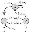
(a) A monoidal transducer $\mathcal{A}$

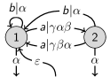
(b) A hypothesis transducer built when learning $\mathcal{A}$

Figure 1: Two transducers: unlike automata, the transitions are also labelled with output words.

Consider for instance the partial function recognized by the minimal transducer $\mathcal{A}$ of Figure 1(a) over the input alphabet $A=\{a,b\}$ and output alphabet $\Sigma=\{\alpha,\beta,\gamma\}$. We write this function $\mathcal{L}({\triangleright}{-}{\triangleleft}):A^{*}\rightarrow\Sigma^{*}\sqcup\{\bot\}$, and let $e\in A^{*}$ and $\epsilon\in\Sigma^{*}$ stand for the respective empty words over these two alphabets. To learn $\mathcal{A}$, the algorithm maintains a subset $Q\subset A^{*}$ of prefixes of input words and a subset $T\subset A^{*}$ of suffixes of input words, and keeps track of the restriction of $\mathcal{L}({\triangleright}{-}{\triangleleft})$ to words in $QT\cup QAT$. The prefixes in $Q$ will be made into states of the hypothesis transducer, and two prefixes $q,q^{\prime}\in Q$ will correspond to two different states if there is a suffix $t\in T$ such that $\mathcal{L}({\triangleright}{qt}{\triangleleft})\neq\mathcal{L}({\triangleright}{q^{\prime}t}{\triangleleft})$. Informally, closure then holds when for any state $q\in Q$ and input letter $a\in A$ an $a$-transition to some state $q^{\prime}\in Q$ can always be built; consistency holds when there is always at most one consistent choice for such a $q^{\prime}$ and when the newly-built $a$-transition can be equipped with an output word. The execution of the learning algorithm for the function recognized by $\mathcal{A}$ would thus look like the following.

The algorithm starts with $Q=T=\{e\}$ only consisting of the empty input word. In a hypothesis transducer, we would want $e\in Q$ to correspond to the initial state, and the output value produced by the initial transition to be the longest common prefix $\Lambda(e)$ of each $\mathcal{L}({\triangleright}{et}{\triangleleft})$ for $t\in T$, here $\Lambda(e)=\alpha$. But the longest common prefix $\Lambda(a)$ of each $\mathcal{L}({\triangleright}{at}{\triangleleft})$ for $t\in T$ is $\gamma\alpha\beta\alpha$, of which $\Lambda(e)$ is not a prefix: it is not possible to make the output of the first $a$-transition so that following the initial transition and then the $a$-transition produces a prefix of $\Lambda(a)$! This is a first kind of consistency issue, which we solve by adding $a$ to $T$, turning $\Lambda(e)$ into the empty output word $\epsilon$ and $\Lambda(a)$ into $\gamma\alpha\beta$.

Now $Q=\{e\}$ and $T=\{e,a\}$. The initial transition should go into the state corresponding to $e$ and output $\Lambda(e)=\epsilon$, the final transition from this state should output $\Lambda(e)^{-1}\mathcal{L}({\triangleright}{e}{\triangleleft})=\alpha$, the $a$-transition from this state should output $\Lambda(e)^{-1}\Lambda(a)=\gamma\alpha\beta$, and this $a$-transition followed by a final transition should output $\Lambda(e)^{-1}\mathcal{L}({\triangleright}{a}{\triangleleft})=\gamma\alpha\beta\alpha$. This $a$-transition should moreover lead to a state from which another $a$-transition followed by a final transition outputs $\Lambda(a)^{-1}\mathcal{L}({\triangleright}{aa}{\triangleleft})=\gamma\beta\alpha^{2}$: in particular, it cannot lead back to the state corresponding to $e$, because $\gamma\beta\alpha^{2}\neq\gamma\alpha\beta\alpha$. But this state is the only state accounted for by $Q$, so now we have no candidate for its successor when following the $a$-transition! This is a closure issue, which we solve by adding $a$ to $Q$, the corresponding new state then being the candidate successor we were looking for.

Once $Q=T=\{e,a\}$, there are no closure nor consistency issues and we may thus build the hypothesis transducer given by Figure 1(b): it coincides with $\mathcal{A}$ on $QA\cup QAT$. Submitting it to the oracle we learn that this transducer is not the one we are looking for, and we get as counter-example the input word $bb$, which indeed satisfies $\mathcal{L}(\triangleright bb\triangleleft)=\bot$ and yet for which our hypothesis transducer produced the output word $\alpha^{3}$: we thus add $bb$ and its prefixes to $Q$.

With $Q=\{e,a,b,bb\}$ and $T=\{e,a\}$ there is another kind of consistency issue, because the states corresponding to $e$ and $b$ are not distinguished by $T$ ($\Lambda(e)^{-1}\mathcal{L}({\triangleright}{et}{\triangleleft})=\Lambda(b)^{-1}\mathcal{L}({\triangleright}{bt}{\triangleleft})$ for all $t\in T$) and should thus be merged in the hypothesis transducer, yet this is not the case of their candidate successors when following an additional $b$-transition ($\mathcal{L}({\triangleright}{ebe}{\triangleleft})=\alpha$ yet $\mathcal{L}({\triangleright}{bbe}{\triangleleft})=\bot$ is undefined)! This issue is solved by adding $b$ to $T$, after which there are again no closure nor consistency issues and we may thus build $\mathcal{A}$ as our new hypothesis transducer. The algorithm finally stops as the oracle confirms that we found the right transducer.

Transducers with outputs in arbitrary monoids.

In the example above we assumed the output of the transducer consisted of words over the output alphabet $\Sigma=\{\alpha,\beta,\gamma\}$, that is of elements of the free monoid $\Sigma^{*}$. But in some contexts it may be relevant to assume that certain output words can be swapped or can cancel each other out. In other words, transducers may be considered to be monoidal and have output not in a free monoid, but in a quotient of a free monoid. An example of a non-trivial family of monoids that should be interesting to use as the output of a transducer is the family of trace monoids, that are used in concurrency theory to model sequences of executions where some jobs are independent of one another and may thus be run asynchronously: transducers with outputs in trace monoids could be used to programatically schedule jobs. Algebraically, trace monoids are just free monoids where some pairs of letters are allowed to commute. For instance, the transducers of Figure 1 could be considered under the assumption that $\alpha\beta=\beta\alpha$, in which case the states $1$ and $2$ would have the same behavior.

This raises the question of the existence and computability of a minimal monoidal transducer recognizing a function with output in an arbitrary monoid. In [Ger18], Gerdjikov gave some conditions on the output monoid for minimal monoidal transducers to exist and be unique up to isomorphism, along with a minimization algorithm that generalizes the one for (non-monoidal) transducers. This question had also been addressed in [Eis03], although in a less satisfying way as the minimization algorithm relied on the existence of stronger oracles. Yet, to the best of the author’s knowledge, no work has addressed the problem of learning minimal monoidal transducers through membership and equivalence queries.

As all monoids are quotients of free monoids, a first solution would of course be to consider the target function to have output in a free monoid, learn the minimal (non-monoidal) transducer recognizing this function using Vilar’s algorithm, and only then consider the resulting transducer to have output in a non-free monoid and minimize it using Gerdjikov’s minimization algorithm. But this solution is unsatisfactory as, during the learning phase, it may introduce states that will be optimized away during the minimization phase. For instance, learning the function recognized by the transducer $\mathcal{A}$ of Figure 1(a) with the assumption that $\alpha\beta=\beta\alpha$ would first produce $\mathcal{A}$ itself before having its states $1$ and $2$ merged during the minimization phase. Worse still, it is possible to find a partial function with output in a finitely generated quotient monoid $\Sigma^{*}/{\sim}$ and recognized by a finite monoidal transducer, and yet so that, when this function is considered to have output in $\Sigma^{*}$, Vilar’s algorithm may not even terminate if, when answering membership queries, the oracle does not carefully choose the representatives in $\Sigma^{*}$ of each equivalence class in $\Sigma^{*}/{\sim}$:

Lemma 1.

Let $A=\{a\}$, $\Sigma=\{\alpha,\beta,\gamma\}$, let $\Sigma^{*}/{\sim}$ be the monoid given by the presentation $\langle\Sigma\mid\alpha\beta=\beta\alpha\rangle$ and let $\pi:\Sigma^{*}\rightarrow\Sigma^{*}/{\sim}$ be the corresponding quotient. Consider the function $f:A^{*}\rightarrow\Sigma^{*}/{\sim}$ that maps $a^{n}$ to $\alpha^{n}\beta^{n}\gamma=(\alpha\beta)^{n}\gamma$.

$f$ is recognized by a finite transducer with outputs in $\Sigma^{*}/{\sim}$, yet learning a transducer that recognizes any function $f^{\prime}:A^{*}\rightarrow\Sigma^{*}$ such that $f=f^{\prime}\circ\pi$ with Vilar’s algorithm will never terminate if the oracle replies to the membership query for $a^{n}$ with $\alpha^{n}\beta^{n}\gamma\in\Sigma^{*}$ (which differs from $(\alpha\beta)^{n}\gamma$ in $\Sigma^{*}$ but not in $\Sigma^{*}/{\sim}$).

Proof 1.1.

$f$ is recognized by the $(\Sigma^{*}/{\sim})$-transducer (Section 3.2) with one state $s$ that is initial, initial value $\upsilon_{0}=\epsilon$, transition function $a\odot s=(\alpha\beta,s)$ and termination function $t(s)=\gamma$.

Consider now the run of Vilar’s algorithm (Algorithm 2 with $M=\Sigma^{*}$ and ${M}^{\times}=\{e\}$) with the oracle answering the membership query for $a^{n}$ with $f^{\prime}(a^{n})=\alpha^{n}\beta^{n}\gamma$. We start with $Q=T=\{e\}$, $\Lambda(e)=\gamma$, $\Lambda(a)=\alpha\beta\gamma$ and $R(e,e)=R(a,e)=\epsilon$, where $\Lambda(w)$ for $w\in Q\cup QA$ is the longest common prefix of the $\{f^{\prime}(wt)\mid t\in T\}$ and $R(w,t)$ is the suffix such that $f^{\prime}(wt)=\Lambda(w)R(w,t)$.

Since $\Lambda(e)=\gamma$ is not a prefix of $\Lambda(a)=\alpha\beta\gamma$, there is a consistency issue and we add $a$ to $T$. Taking $n=0$, we are now in the configuration $C_{n}$ given by $Q=Q_{n}=\{a^{k}\mid k\leq n\}$, $T=\{e,a\}$, and $\Lambda(a^{k})=\alpha^{k}$, $R(a^{k},e)=\beta^{k}\gamma$ and $R(a^{k},a)=\alpha\beta^{k+1}\gamma$ for every $k\leq n+1$ (since the oracle replies to the membership query for $a^{k}$ with $\alpha^{k}\beta^{k}\gamma$ and to that for $a^{k}a$ with $\alpha^{k+1}\beta^{k+1}\gamma$).

Suppose now we are in the configuration $C_{n}$ for some $n\in\mathbb{N}$. Then there is a closure issue, since for all $k\leq n$, $R(a^{k},e)=\beta^{k}\gamma\neq\beta^{n+1}\gamma=R(a^{n+1},e)$. We thus add $a^{n+1}$ to $Q$. To compute $\Lambda(a^{n+2})$, $R(a^{n+2},e)$ and $R(a^{n+2},a)$, we make a membership query for $a^{n+3}$: the oracle answers with $f^{\prime}(a^{n+3})=\alpha^{n+3}\beta^{n+3}\gamma$. The longest common prefix of $f^{\prime}(a^{n+2})=\Lambda(a^{n+1})R(a^{n+1},a)=\alpha^{n+2}\beta^{n+2}\gamma$ and $f^{\prime}(a^{n+2}a)=\alpha^{n+3}\beta^{n+3}\gamma$ is thus $\alpha^{n+2}$, and the corresponding suffixes are $R(a^{n+2},e)=\beta^{n+2}\gamma$ and $R(a^{n+2},a)=\alpha\beta^{n+3}\gamma$: we are now in the configuration $C_{n+1}$.

Hence the run of the algorithm never terminates and never even reaches an equivalence query, as it must first go through all the configurations $C_{n}$ for $n\in\mathbb{N}$.

The idea of finding such an example was suggested by an anonymous reviewer whom the author thanks.

A more satisfactory solution would hence do away with the minimization phase and instead use the assumptions on the output monoid during the learning phase to directly produce the minimal monoidal transducer.

Structure and contributions.

In this work we thus study the problem of generalizing Vilar’s algorithm to monoidal transducers. To this aim, we first recall in Section 2 the categorical framework of Colcombet, Petrişan and Stabile for learning minimal transition systems [CPS20]. This framework encompasses both Angluin’s and Vilar’s algorithms, as well as a similar algorithm for weighted automata [BV94, BV96]. We use this specific framework because, while others exist, they either do not encompass transducers or require stronger assumptions [BKR19, US20, vSS20]. In Section 3 we then instantiate this framework to retrieve monoidal transducers as transition systems whose state-spaces live in a certain category (Section 3.2). Studying the existence of specific structures in this category — namely, powers of the terminal object (Section 3.3) and factorization systems (Section 3.4) — we then give conditions for the framework to apply and hence for the minimal monoidal transducers to exist and be computable.

This paper’s contributions are thus the following:

• necessary and sufficient conditions on the output monoid for the categorical framework of Colcombet, Petrişan and Stabile to apply to monoidal transducers are given;

• these conditions mostly overlap those of Gerdjikov, but are nonetheless not equivalent: in particular, they extend the class of output monoids for which minimization is known to be possible, although with a possibly worse complexity bound;

• practical details on the implementation of the abstract monoidal transducer-learning algorithm that results from the categorical framework are given;

• in particular, additional structure on the category in which the framework is provides a neat categorical explanation to both the different kinds of consistency issues that arise in the learning algorithm and the main steps that are taken in every transducer minimization algorithm.

2 Categorical approach to learning minimal automata

In this section we recall (and extend) the definitions and results of Colcombet, Petrişan and Stabile [PC20, CPS21]. We assume basic knowledge of category theory [ML78], but we also focus on the example of deterministic complete automata and on the counter-example of non-deterministic automata. We do not explain it here but the framework also applies to weighted automata [BV94, BV96, Sch61] and (non-monoidal) transducers (as generalized in Section 3).

2.1 Automata and languages as functors

Consider the graph $\smash{\mathtt{in}\xrightarrow[]{\triangleright}\overset{{\text{\normalsize$\overset{a}{\curvearrowleft}$}}}{\mathtt{st}}\xrightarrow[]{\triangleleft}\mathtt{out}}$ where $a$ ranges in the input alphabet $A$, and let $\mathcal{I}$, the input category, be the category that it generates: the objects are the vertices of this graph and the morphisms paths between two vertices. $\mathcal{I}$ represents the basic structure of automata as transition systems: $\mathtt{st}$ represents the state-space, $\triangleright$ the initial configuration, each $a:\mathtt{st}\rightarrow\mathtt{st}$ the transition along the corresponding letter, and $\triangleleft$ the output values associated to each state. An automaton is then an instantiation of $\mathcal{I}$ in some output category:

[$(\mathcal{C},X,Y)$-automaton] Given an output category $\mathcal{C}$, a $(\mathcal{C},X,Y)$-automaton is a functor $\mathcal{A}:\mathcal{I}\rightarrow\mathcal{C}$ such that $\mathcal{A}(\mathtt{in})=X$ and $\mathcal{A}(\mathtt{out})=Y$.

[(non-)deterministic automata] If $1=\{*\}$ and $2=\{\bot,\top\}$, a $(\mathbf{Set},1,2)$-automaton $\mathcal{A}$ is a (possibly infinite) deterministic complete automaton: it is given by a state-set $S=\mathcal{A}(\mathtt{st})$, transition functions $\mathcal{A}(a):S\rightarrow S$ for each $a\in A$, an initial state $s_{0}=\mathcal{A}(\triangleright)(*)\in S$ and a set of accepting states $F=\{s\in S\mid\mathcal{A}(\triangleleft)(s)=\top\}\subseteq S$. Similarly, a $(\mathbf{Rel},1,1)$-automaton (where $\mathbf{Rel}$ is the category of sets and relations between them) is a (possibly infinite) non-deterministic automaton: it is given by a state-set $S=\mathcal{A}(\mathtt{st})$, transition relations $\mathcal{A}(a)\subseteq S\times S$, a set of initial states $\mathcal{A}(\triangleright)\subseteq 1\times S\cong S$ and a set of accepting states $\mathcal{A}(\triangleleft)\subseteq S\times 1\cong S$.

[$(\mathcal{C},X,Y)$-language] In the same way, we define a language to be a functor $\mathcal{L}:\mathcal{O}\rightarrow\mathcal{C}$, where $\mathcal{O}$, the category of observable inputs, is the full subcategory of $\mathcal{I}$ on $\mathtt{in}$ and $\mathtt{out}$. In other words, a language is the data of two objects $X=\mathcal{L}(\mathtt{in})$ and $Y=\mathcal{L}(\mathtt{out})$ in $\mathcal{C}$ (in which case we speak of a $(\mathcal{C},X,Y)$-language), and, for each word $w\in A^{*}$, of a morphism $\mathcal{L}(\triangleright w\triangleleft):X\rightarrow Y$. In particular, composing an automaton $\mathcal{A}:\mathcal{I}\rightarrow\mathcal{C}$ with the embedding $\iota:\mathcal{O}\hookrightarrow\mathcal{I}$, we get the language $\mathcal{L}_{\mathcal{A}}=\mathcal{A}\circ\iota$ recognized by $\mathcal{A}$.

[languages] The language recognized by a $(\mathbf{Set},1,2)$-automaton $\mathcal{A}$ is the language recognized by the corresponding complete deterministic automaton: for a given $w\in A^{*}$, $\mathcal{L}_{\mathcal{A}}(\triangleright w\triangleleft)(*)=\top$ if and only if $w$ belongs to the language, and the equality $\mathcal{L}_{\mathcal{A}}(\triangleright w\triangleleft)=\mathcal{A}(\triangleright w\triangleleft)=\mathcal{A}(\triangleright)\mathcal{A}(w)\mathcal{A}(\triangleleft)$ means that we can decide whether $w$ is in the language by checking whether the state we get in by following $w$ from the initial state is accepting. Such a language could also be seen as a set of relations $\mathcal{L}(\triangleright w\triangleleft)\subseteq 1\times 1$, where $*$ is related to itself if and only if $w$ belongs to $\mathcal{L}$. The language recognized by a $(\mathbf{Rel},1,1)$-automaton is thus the language recognized by the corresponding non-deterministic automaton.

[category of automata recognizing a language] Given a category $\mathcal{C}$ and a language $\mathcal{L}:\mathcal{O}\rightarrow\mathcal{C}$, we define the category $\mathbf{Auto}(\mathcal{L})$ whose objects are $(\mathcal{C},\mathcal{L}(\mathtt{in}),\mathcal{L}(\mathtt{out}))$-automata $\mathcal{A}$ recognizing $\mathcal{L}$, and whose morphisms $\mathcal{A}\rightarrow\mathcal{A}^{\prime}$ are natural transformations whose components on $\mathcal{L}(\mathtt{in})$ and $\mathcal{L}(\mathtt{out})$ are the identity. In other words, a morphism of automata is given by a morphism $f:\mathcal{A}(\mathtt{st})\rightarrow\mathcal{A}^{\prime}(\mathtt{st})$ in $\mathcal{C}$ such that $\mathcal{A}^{\prime}(\triangleright)=f\circ\mathcal{A}(\triangleright)$ (it preserves the initial configuration), $\mathcal{A}^{\prime}(a)\circ f=f\circ\mathcal{A}(a)$ (it commutes with the transitions), and $\mathcal{A}^{\prime}(\triangleleft)\circ f=\mathcal{A}(\triangleleft)$ (it preserves the output values).

2.2 Factorization systems and the minimal automaton recognizing a language

[factorization system] In a category $\mathcal{C}$, a factorization system $(\mathcal{E},\mathcal{M})$ is the data of a class of $\mathcal{E}$-morphisms (represented with $\twoheadrightarrow$) and a class of $\mathcal{M}$-morphisms (represented with $\rightarrowtail$) $\mathcal{M}$ such that

• every arrow $f$ in $\mathcal{C}$ may be factored as $f=m\circ e$ with $m\in\mathcal{M}$ and $e\in\mathcal{E}$;

• $\mathcal{E}$ and $\mathcal{M}$ are both stable under composition;

• for every commuting diagram as below where $m\in\mathcal{M}$ and $e\in\mathcal{E}$ there is a unique diagonal fill-in $d:Y_{1}\rightarrow Y_{2}$ such that $u=d\circ e$ and $v=m\circ d$.

In $\mathbf{Set}$ surjective and injective functions form a factorization system $(\mathrm{Surj},\mathrm{Inj})$ such that a map $f:X\rightarrow Y$ factors through its image $f(X)\subseteq Y$. In $\mathbf{Rel}$ a factorization system is given by $\mathcal{E}$-morphisms those relations $r:X\rightarrow Y$ such that every $y\in Y$ is related to some $x\in X$ by $r$, and $\mathcal{M}$-morphisms the graphs of injective functions (i.e. $m\in\mathcal{M}$ if and only if there is an injective function $f$ such that $(x,y)\in m\iff y=f(x)$). A relation $r:X\rightarrow Y$ then factors through the subset $\{y\in Y\mid\exists x\in X,(x,y)\in R\}\subseteq Y$.

Lemma 2 (factorization system on $\mathbf{Auto}(\mathcal{L})$ [PC20, Lemma 2.8]).

Given $\mathcal{L}:\mathcal{I}\rightarrow\mathcal{C}$ and $(\mathcal{E},\mathcal{M})$ a factorization system on $\mathcal{C}$, $\mathbf{Auto}(\mathcal{L})$ has a factorization given by those natural transformations whose components are respectively $\mathcal{E}$- and $\mathcal{M}$-morphisms.

Because of this last result, we use $(\mathcal{E},\mathcal{M})$ to refer both to a factorization on $\mathcal{C}$ and to its extensions to categories of automata.

[minimal object] When a category $\mathcal{C}$, equipped with a factorization system $(\mathcal{E},\mathcal{M})$, has both an initial object $I$ and a final object $F$ (for every object $X$ there is exactly one morphism $I\rightarrow X$ and one morphism $X\rightarrow F$), we define its $(\mathcal{E},\mathcal{M})$-minimal object $\operatorname{Min}{}$ to be the one that $(\mathcal{E},\mathcal{M})$-factors the unique arrow $I\rightarrow F$ as $I\twoheadrightarrow\operatorname{Min}{}\rightarrowtail F$. For every object $X$ we also define $\operatorname{Reach}X$ and $\operatorname{Obs}X$ by the $(\mathcal{E},\mathcal{M})$-factorizations $I\twoheadrightarrow\operatorname{Reach}X\rightarrowtail X$ and $X\twoheadrightarrow\operatorname{Obs}X\rightarrowtail F$.

Proposition 3 (uniqueness of the minimal object [PC20, Lemma 2.3]).

The minimal object of a category $\mathcal{C}$ is unique up to isomorphism, so that for every other object $X$, $\operatorname{Min}\cong\operatorname{Obs}(\operatorname{Reach}X)\cong\operatorname{Reach}(\operatorname{Obs}X)$: there are in particular spans $X\leftarrowtail\operatorname{Reach}X\twoheadrightarrow\operatorname{Min}$ and co-spans $\operatorname{Min}\rightarrowtail\operatorname{Obs}X\twoheadleftarrow X$. It is in that last sense that $\operatorname{Min}$ is $(\mathcal{E},\mathcal{M})$-smaller than every other object $X$, and is thus minimal.

[initial, final and minimal automata [PC20, Example 3.1]] Since $\mathbf{Set}$ is complete and cocomplete, the category of $(\mathbf{Set},1,2)$-automata recognizing a language $\mathcal{L}:\mathcal{I}\rightarrow\mathbf{Set}$ has an initial, a final and a minimal object. The initial automaton has state-set $A^{*}$, initial state $\epsilon\in A^{*}$, transition functions $\delta_{a}(w)=wa$ and accepting states the $w\in A^{*}$ such that $w$ is in $\mathcal{L}$. Similarly, the final automaton has state-set $2^{A^{*}}$, initial state $\mathcal{L}$, transition functions $\delta_{a}(L)=a^{-1}L$ and accepting states the $L\in 2^{A^{*}}$ such that $\epsilon$ is in $L$. The minimal automaton for the factorization system of Section 2.2 thus has the Myhill-Nerode equivalence classes for its states. It is unique up to isomorphism and its $(\mathcal{E},\mathcal{M})$-minimality ensures that it is the complete deterministic automaton with the smallest state-set that recognizes $\mathcal{L}$: it is in particular finite as soon as $\mathcal{L}$ is recognized by a finite automaton.

On the contrary, there is no good notion of a unique minimal non-deterministic automaton recognizing a regular ($(\mathbf{Rel},1,1)$-) language $\mathcal{L}$. $\mathbf{Auto}(\mathcal{L})$ does have an initial and a final object: the initial automaton is the initial deterministic automaton recognizing $\mathcal{L}$, and the final automaton is the (non-deterministic) transpose of this initial automaton. But there is no factorization system that gives rise to a meaningful minimal object: for instance, the minimal object for the factorization system described in Section 2.2 has for state-set the set of suffixes of words in $\mathcal{L}$.

Notice how in Proposition 3 the initial and final $(\mathbf{Set},1,2)$-automata have for respective state-sets $A^{*}$, the disjoint union of $|A^{*}|$ copies of $1$, and $2^{A^{*}}$, the cartesian product of $|A^{*}|$ copies of $2$. A similar result holds for non-deterministic automata and generalizes as Theorem 4, itself summarized by the diagram below, where $\kappa$ and $\pi$ are the canonical inclusion and projections and $[-]$ and $\langle-\rangle$ are the copairing and pairing of arrows.

Theorem 4 ([PC20, Lemma 3.2]).

Given a countable alphabet $A$ and a language $\mathcal{L}:\mathcal{I}\rightarrow\mathcal{C}$,

• if $\mathcal{C}$ has all countable copowers of $\mathcal{L}(\mathtt{in})$ then $\mathbf{Auto}(\mathcal{L})$ has an initial object $\mathcal{A}^{init}(\mathcal{L})$ with $\mathcal{A}^{init}(\mathcal{L})(\mathtt{st})=\coprod_{A^{*}}\mathcal{L}(\mathtt{in})$;

• dually if $\mathcal{C}$ has all countable powers of $\mathcal{L}(\mathtt{out})$ then $\mathbf{Auto}(\mathcal{L})$ has a final object $\mathcal{A}^{final}(\mathcal{L})$ with $\mathcal{A}^{final}(\mathcal{L})(\mathtt{st})=\prod_{A^{*}}\mathcal{L}(\mathtt{out})$;

• hence when both of the previous items hold and $\mathcal{C}$ comes equipped with a factorization system $(\mathcal{E},\mathcal{M})$, $\mathbf{Auto}(\mathcal{L})$ has an $(\mathcal{E},\mathcal{M})$-minimal object $\operatorname{Min}\mathcal{L}$.

We now have all the ingredients to define algorithms for computing the minimal automaton recognizing a language. But since we will also want to prove the termination of these algorithms, we need an additional notion of finiteness.

[$\mathcal{E}$-artinian and $\mathcal{M}$-noetherian objects [CPS20, Definition 24]] In a category $\mathcal{C}$ equipped with a factorization system $(\mathcal{E},\mathcal{M})$, an object $X$ is said to be $\mathcal{M}$-noetherian if every strict chain of $\mathcal{M}$-subobjects is finite: if $(x_{n}:X_{n}\rightarrowtail X)_{n\in\mathbb{N}}$ and $(m_{n}:X_{n}\rightarrowtail X_{n+1})$ form the commutative diagram

then only finitely many of the $m_{n}$’s may not be isomorphisms. Dually, $X$ is $\mathcal{E}$-artinian if $X^{\mathrm{op}}$ is $\mathcal{E}^{\mathrm{op}}$-noetherian in $\mathcal{C}^{\mathrm{op}}$, that is if every strict cochain of $\mathcal{E}$-quotients of $X$ is finite.

While Colcombet, Petrişan and Stabile do not give complexity results for their algorithm, it is straightforward to do so, hence we extend their definition so that it also measures the size of an object in $\mathcal{C}$.

[co-$\mathcal{E}$- and $\mathcal{M}$-lengths] For a fixed $x_{0}:X_{0}\rightarrowtail X$, we call $\mathcal{M}$-length of $x_{0}$, written $\operatorname{length}_{\mathcal{M}}x_{0}$, the (possibly infinite) supremum of the lengths (the number of pairs of consecutive subobjects) of strict chains of $\mathcal{M}$-subobjects of $X$ that start with $x_{0}$. Dually, we call co-$\mathcal{E}$-length of an $\mathcal{E}$-quotient $x_{0}:X\twoheadrightarrow X_{0}$ the (possibly infinite) quantity $\operatorname{colength}_{\mathcal{E}}x_{0}=\operatorname{length}_{\mathcal{E}^{\mathrm{op}}}x_{0}^{\mathrm{op}}$.

In $\mathbf{Set}$, $X$ is finite if and only if it is $\mathrm{Inj}$-noetherian iff it is $\mathrm{Surj}$-artinian, and in that case for $Y\subseteq X$ we have $\operatorname{colength}_{\mathrm{Surj}}(X\twoheadrightarrow Y)=\operatorname{length}_{\mathrm{Inj}}(Y\rightarrowtail X)=|X-Y|$. Note that the co-$E$- and $\mathcal{M}$-lengths need not be equal: see for instance the factorization system we define for monoidal transducers in Section 3.4, for which the co-$\mathcal{E}$- and $\mathcal{M}$-lengths are computed in Lemmas 18 and 19.

2.3 Learning

In this section, we fix a language $\mathcal{L}:\mathcal{O}\rightarrow\mathcal{C}$ and a factorization system $(\mathcal{E},\mathcal{M})$ of $\mathcal{C}$ that extends to $\mathbf{Auto}(\mathcal{L})$, and we assume that $\mathcal{C}$ has countable copowers of $\mathcal{L}(\mathtt{in})$ and countable powers of $\mathcal{L}(\mathtt{out})$ so that Theorem 4 applies. Our goal is to compute $\operatorname{Min}\mathcal{L}$ with the help of an oracle answering two types of queries: the function $\textsc{Eval}_{\mathcal{L}}$ processes membership queries, and, for a given input word $w\in A^{*}$, outputs $\mathcal{L}(\triangleright w\triangleleft)$; while $\textsc{Equiv}_{\mathcal{L}}$ processes equivalence queries, and, for a given hypothesis $(\mathcal{C},\mathcal{L}(\mathtt{in}),\mathcal{L}(\mathtt{out}))$-automaton $\mathcal{A}$, decides whether $\mathcal{A}$ recognizes $\mathcal{L}$, and, if not, outputs a counter-example $w\in A^{*}$ such that $\mathcal{L}(\triangleright w\triangleleft)\neq(\mathcal{A}\circ\iota)(\triangleright w\triangleleft)$.

For $(\mathbf{Set},1,2)$-automata, if the language is regular this problem is solved using Angluin’s L* algorithm [Ang87]. It works by maintaining a set of prefixes $Q$ and of suffixes $T$ and, using $\textsc{Eval}_{\mathcal{L}}$, incrementally building a table $L:Q\times(A\cup\{\epsilon\})\times T\rightarrow 2$ that represents partial knowledge of $\mathcal{L}$ until it can be made into a (minimal) automaton. This automaton is then submitted to $\textsc{Equiv}_{\mathcal{L}}$ when some closure and consistency conditions hold: if the automaton is accepted it must be $\operatorname{Min}\mathcal{L}$, otherwise the counter-example is added to $Q$ and the algorithm loops over. The FunL* algorithm (Algorithm 1, algorithm 1) generalizes this to arbitrary $(\mathcal{C},\mathcal{L}(\mathtt{in}),\mathcal{L}(\mathtt{out}))$, and in particular also encompasses Vilar’s algorithm for learning (non-monoidal) transducers, which was described in Section 1 [CPS20].

Instead of maintaining a table, the FunL* algorithm maintains a biautomaton: if $Q\subseteq A^{*}$ is prefix-closed ($wa\in Q\Rightarrow w\in Q$) and $T\subseteq A^{*}$ is suffix-closed ($aw\in T\Rightarrow w\in T$), a $(Q,T)$-biautomaton is, similarly to an automaton, a functor $\mathcal{A}:\mathcal{I}_{Q,T}\rightarrow\mathcal{C}$, where $\mathcal{I}_{Q,T}$ is now the category freely generated by the graph where $a$, $q$ and $t$ respectively range in $A$, $Q$ and $T$, and where we also require the diagrams below to commute, the left one whenever $qa\in Q$ and the right one whenever $at\in T$.

A $(Q,T)$-biautomaton may thus process a prefix in $Q$ and get in a state in $\mathcal{A}(\mathtt{st}_{1})$, follow a transition along $A\cup\{\epsilon\}$ to go in $\mathcal{A}(\mathtt{st}_{2})$, and output a value for each suffix in $T$. The category of biautomata recognizing $\mathcal{L}_{Q,T}$ ($\mathcal{L}$ restricted to words in $QT\cup QAT$) is written $\mathbf{Auto}_{Q,T}(\mathcal{L})$. A result similar to Theorem 4 also holds for biautomata [CPS20, Lemma 18], and the initial and final biautomata are then made of finite copowers of $\mathcal{L}(\mathtt{in})$ and finite powers of $\mathcal{L}(\mathtt{out})$ (when these exist). Writing $\left.{Q}\middle/{T}\right.$ for the $(\mathcal{E},\mathcal{M})$-factorization of the canonical morphism $\langle[\mathcal{L}(\triangleright qt\triangleleft)]_{q\in Q}\rangle_{t\in T}:\coprod_{Q}\mathcal{L}(\mathtt{in})\rightarrow\prod_{T}\mathcal{L}(\mathtt{out})$, the minimal biautomaton recognizing $\mathcal{L}_{Q,T}$ then has state-spaces $(\operatorname{Min}\mathcal{L}_{Q,T})(\mathtt{st}_{1})=\left.{Q}\middle/{(T\cup AT)}\right.$ and $(\operatorname{Min}\mathcal{L}_{Q,T})(\mathtt{st}_{2})=\left.{(Q\cup QA)}\middle/{T}\right.$. The table, represented by the morphism $\langle[\mathcal{L}(\triangleright qt\triangleleft)]_{q\in Q}\rangle_{t\in T}$, may be fully computed using $\textsc{Eval}_{\mathcal{L}}$, and hence so can be the minimal $(Q,T)$-biautomaton.

A biautomaton $\mathcal{B}$ can then be merged into a hypothesis $(\mathcal{C},\mathcal{L}(\mathtt{in}),\mathcal{L}(\mathtt{out}))$-automaton precisely when $\mathcal{B}(\epsilon)$ is an isomorphism, i.e. both an $\mathcal{E}$- and an $\mathcal{M}$-morphism (a factorization system necessarily satisfies that $\mathrm{Iso}=\mathcal{E}\cap\mathcal{M}$): this encompasses respectively the closure and consistency conditions that need to hold in the L*-algorithm (and its variants) for the table that is maintained to be merged into a hypothesis automaton.

Theorem 5 ([CPS20, Theorem 26]).

Algorithm 1 is correct. If $(\operatorname{Min}\mathcal{L})(\mathtt{st})$ is $\mathcal{M}$-noetherian and $\mathcal{E}$-artinian, the algorithm also terminates.

While Colcombet, Petrişan and Stabile do not give a bound on the actual running time of their algorithm, it is straightforward to extend their proof to show that the number of updates to $Q$ and $T$ (hence in particular of calls to $\textsc{Equiv}_{\mathcal{L}}$) is linear in the size of $(\operatorname{Min}\mathcal{L})(\mathtt{st})$, itself defined through Theorem 4.

Algorithm 1 The FunL*-algorithm

0:  $\textsc{Eval}_{\mathcal{L}}$ and $\textsc{Equiv}_{\mathcal{L}}$

0:  $\operatorname{Min}(\mathcal{L})$

1:  $Q=T=\{\epsilon\}$

2:  loop

3:     while $\epsilon_{Q,T}^{min}$ is not an isomorphism do

4:        if $\epsilon_{Q,T}^{min}$ is not an $\mathcal{E}$-morphism then

5:           find $qa\in QA$ such that $\left.{Q}\middle/{T}\right.\rightarrowtail\left.{(Q\cup\{qa\})}\middle/{T}\right.$ is not an $\mathcal{E}$-morphism; add it to $Q$

6:        else if $\epsilon_{Q,T}^{min}$ is not an $\mathcal{M}$-morphism then

7:           find $at\in AT$ such that $\left.{Q}\middle/{(T\cup\{at\})}\right.\twoheadrightarrow\left.{Q}\middle/{T}\right.$ is not an $\mathcal{M}$-morphism; add it to $T$

8:        end if

9:     end while

10:     merge $\operatorname{Min}\mathcal{L}_{Q,T}$ into $\mathcal{H}_{Q,T}\mathcal{L}$

11:     if $\textsc{Equiv}_{\mathcal{L}}(\mathcal{H}_{Q,T}\mathcal{L})$ outputs some counter-example $w$ then

12:        add $w$ and its prefixes to $Q$

13:     else

14:        return  $\mathcal{H}_{Q,T}\mathcal{L}$

15:     end if

16:  end loop

3 The category of monoidal transducers

We now study a specific family of transition systems, monoidal transducers, through the lens of category theory, so as to be able to apply the framework of Colcombet, Petrişan and Stabile. In Section 3.1, we first rapidly recall the notion of monoid. We then define the category of monoidal transducers recognizing a language in Section 3.2, and study how it fits into the framework of Section 2: the initial transducer is given in Corollary 8, conditions for the final transducer to exist are described in Section 3.3, and factorization systems are tackled in Section 3.4.

3.1 Monoids

Let us first recall definitions relating to monoids, and fix some notations. Most of these are standard in the monoid literature, only coprime-cancellativity (Section 3.1) and noetherianity (Section 3.1) are uncommon.

[monoid] A monoid $(M,\epsilon_{M},{\otimes_{M}})$ is a set $M$ equipped with a binary operation ${\otimes_{M}}$ (often called the product) that is associative ($\forall u,v,w\in M,u\otimes_{M}(v\otimes_{M}w)=(u\otimes_{M}v)\otimes_{M}w$) and has $\epsilon_{M}$ as unit element ($\forall u\in M,u\otimes_{M}\epsilon_{M}=\epsilon_{M}\otimes_{M}u=u$). When non-ambiguous, it is simply written $(M,\epsilon,{\otimes})$ or even $M$, and the symbol for the binary operation may be omitted.

The dual of $(M,\epsilon,{\otimes})$, written $({M}^{op},{\epsilon}^{op},{\otimes}^{op})$, has underlying set ${M}^{op}=M$ and identity ${\epsilon}^{op}=\epsilon$, but symmetric binary operation: $\forall u,v\in M,u\otimes^{op}v=v\otimes u$.

The dual of a monoid is mainly used here for the sake of conciseness: whenever we define some “left-property”, the corresponding “right-property” is defined as the left-property but in the dual monoid. Note that when $M$ is commutative it is its own dual and the left- and right-properties coincide.

[invertibility] An element $x$ of a monoid $M$ is right-invertible when there is a $y\in M$ such that $xy=\epsilon$, and $y$ is then called the right-inverse of $x$. It is left-invertible when it is right-invertible in ${M}^{op}$, and the corresponding right-inverse is called its left-inverse. When $x$ is both right- and left-invertible, we say it is invertible. In that case its right- and left-inverse are equal: this defines its inverse, written ${x}^{-1}$. The set of invertible elements of $M$ is written ${M}^{\times}$.

Two families $(u_{i})_{i\in I}$ and $(v_{i})_{i\in I}$ indexed by some non-empty set $I$ are equal up to invertibles on the left when there is some invertible $x\in M$ such that $\forall i\in I,u_{i}=xv_{i}$.

[divisibility] An element $u$ of a monoid $M$ left-divides a family $w=(w_{i})_{i\in I}$ of $M$ indexed by some set $I$ when there is a family $(v_{i})_{i\in I}$ such that $\forall i\in I,uv_{i}=w_{i}$, and we say that $u$ is a left-divisor of $w$. It right-divides it when it left-divides it in ${M}^{op}$, and in that case $u$ is called a right-divisor of $w$.

A greatest common left-divisor (or left-gcd) of the family $w$ is a left-divisor of $w$ that is left-divided by all others left-divisors of $w$.

A family $w$ is said to be left-coprime when it has $\epsilon$ as a left-gcd, i.e. when all its left-divisors (or equivalently one of its left-gcds, if there is one) are right-invertible.

We speak of greatest common left-divisors because, while there may be many such elements for a fixed family $\omega$, they all left-divide one another and are thus equivalent in some sense.

[cancellativity] A monoid $M$ is said to be left-cancellative when for any families $(u_{i})_{i\in I}$ and $(v_{i})_{i\in I}$ of $M$ indexed by some set $I$ and for any $w\in M$, $u=v$ as soon as $wu_{i}=wv_{i}$ for all $i\in I$. If this only implies $u_{i}=xv_{i}$ for some $x\in{M}^{\times}$, we instead say that $M$ is left-cancellative up to invertibles on the left.

Similarly, $M$ is said to be right-coprime-cancellative when for any $u,v\in M$ and any left-coprime family $(w_{i})_{i\in I}$ indexed by some set $I$, $u=v$ as soon as $uw_{i}=vw_{i}$ for all $i\in I$.

[noetherianity] A monoid $M$ is right-noetherian when for any sequences $(u_{n})_{n\in\mathbb{N}}$ and $(v_{n})_{n\in\mathbb{N}}$ of $M$ such that $v_{n}=v_{n+1}u_{n}$ for all $n\in\mathbb{N}$, there is some $n\in\mathbb{N}$ such that $u_{n}$ is invertible.

In this case, we write $\operatorname{rk}v$ for the rank of $v$, the (possibly infinite) supremum of the numbers of non-invertibles in a sequence $(u_{n})_{n\in\mathbb{N}}$ that satisfies $v_{n}=v_{n+1}u_{n}$ for a sequence $(v_{n})_{n\in\mathbb{N}}$ with $v_{0}=v$.

In other words, a monoid is right-noetherian when it has no strict infinite chains of right-divisors (in the definition above, each $u_{n}\cdots u_{0}$ right-divides $v_{0}$). Note that $\operatorname{rk}(uv)\leq\operatorname{rk}u+\operatorname{rk}v$, and $\operatorname{rk}:M\rightarrow\mathbb{N}$, and if this is an equality $M$ is said to be graded.

Noetherianity will be used to ensure that fixed-point algorithms terminate, hence we will often assume that the monoids we work with satisfy some noetherianity properties. We therefore state two additional lemmas making it easier to work with noetherian monoids. They both assume $M$ to be right-noetherian but the dual results also stand.

Lemma 6.

$M$ is right-noetherian if and only if for any sequences $(u_{n})_{n\in\mathbb{N}}$ and $(v_{n})_{n\in\mathbb{N}}$ of $M$ such that $v_{n}=v_{n+1}u_{n}$ for all $n\in\mathbb{N}$, there is some $n\in\mathbb{N}$ such that for all $i\geq n$, $u_{i}$ is invertible.

Proof 3.1.

The reverse implication is trivial. Now assume $M$ right-noetherian, and consider $(u_{n})_{n\in\mathbb{N}}$ and $(v_{n})_{n\in\mathbb{N}}$ such that $v_{n}=v_{n+1}u_{n}$ for all $n\in\mathbb{N}$. Consider the set $I=\{i_{0}<i_{1}<\ldots\}$ of all the indices $i$ such that $u_{i}$ is not invertible and, letting $i_{-1}=-1$, define $u_{n}^{\prime}=u_{i_{n}}\cdots u_{i_{n-1}+1}$ and $v_{n}^{\prime}=v_{i_{n}+1}$ for all $n\in\mathbb{N}$. Then $u_{n}^{\prime}$ is never invertible because $u_{i_{n}}$ is not but $u_{i_{n}-1},\ldots,u_{i_{n-1}+1}$ are (by definition), yet we still have by induction that $v_{n}^{\prime}=v_{n+1}^{\prime}u_{n}^{\prime}$. Since $M$ is left-noetherian, $I$ must be finite hence there is some $n\in\mathbb{N}$ such that for all $i\geq n$, $m_{i}$ is invertible.

Lemma 7.

If $M$ is right-noetherian then all its right- and left-invertibles are invertible.

Proof 3.2.

Assume $M$ right-noetherian and consider some $x$ that is right-invertible with $x_{r}$ its right-inverse. For $n\in\mathbb{N}$, set $u_{2n}=x_{r}$, $v_{2n}=\epsilon$ and $u_{2n+1}=v_{2n+1}=x$. Then $v_{n}=v_{n+1}u_{n}$ for all $n\in\mathbb{N}$ hence by right-noetherianity $x$ is invertible. If $x$ is left-invertible instead, its left-inverse is right-invertible hence invertible and therefore so is $x$.

The canonical example of a monoid is the free monoid $A^{*}$ over an alphabet $A$, whose elements are words with letters in $A$, whose product is the concatenation of words and whose unit is the empty word. Notice that the alphabet $A$ may be infinite. The left-divisibility relation is the prefix one, and the left-gcd is the longest common prefix.

The free commutative monoid $A^{\oast}$ over $A$ has elements the functions $A\rightarrow\mathbb{N}$ with finite support, product $(f\otimes g)(a)=f(a)+g(a)$ and unit the zero function $a\mapsto 0$. It is commutative ($f\otimes g=g\otimes f$) hence is its own dual: the divisibility relation is the pointwise order inherited from $\mathbb{N}$ and the greatest common divisor is the pointwise infimum.

These two monoids are examples of trace monoids over some $A$, defined as quotients of $A^{*}$ by commutativity relations on letters (for $A^{\oast}$, all the pairs of letters are required to commute, and for $A^{*}$ none are). Trace monoids have no non-trivial right- or left-invertible elements, are all left-cancellative, right-coprime-cancellative and right-noetherian, and the rank of a word is simply its number of letters.

Another family of examples is that of groups, monoids where all elements are invertible. Again, all groups are left-cancellative, right-coprime-cancellative and right-noetherian.

A final monoid of interest is $(E,{\vee},\bot)$ for $E$ any join-semilattice with a bottom element $\bot$. In this commutative monoid, the divisibility relation is the partial order on $E$, and the gcd, when it exists, is the infimum. This example shows that a monoid can be coprime-cancellative without being cancellative nor noetherian: this is for instance the case when $E=\mathbb{R}_{+}$ (this counter-example was pointed out to the author by Thomas Colcombet).

3.2 Monoidal transducers as functors

In the rest of this paper we fix a countable input alphabet $A$ and an output monoid $(M,\epsilon,\otimes)$. To differentiate between elements of $A^{*}$ and elements of $M$, we write the former with Latin letters ($a,b,c,\ldots$ for letters and $u,v,w,\ldots$ for words) and the latter with Greek letters ($\alpha,\beta,\gamma,\ldots$ for generating elements and $\upsilon,\nu,\omega,\ldots$ for general elements). In particular the empty word over $A$ is denoted $e$ while the unit of $M$ is still written $\epsilon$. We now define our main object of study, $M$-monoidal transducers.

[monoidal transducer] A monoidal transducer is a tuple $(S,(\upsilon_{0},s_{0}),t,(-\odot a)_{a\in A})$ where $S$ is a set of states; $(\upsilon_{0},s_{0})\in M\times S\sqcup\{\bot\}$ is the (possibly undefined) pair of the initialization value and initial state; $t:S\rightarrow M\sqcup\{\bot\}$ is the partial termination function; $s\odot a\in M\times S\sqcup\{\bot\}$ for $a\in A$ may be undefined, and its two components, $-\ocircle a:S\rightarrow M\sqcup\{\bot\}$ and $-\cdot a:S\rightarrow S\sqcup\{\bot\}$, are respectively called the partial production function and the partial transition function along $a$.

Figure 2 is a graphical representation of a monoidal transducer that takes its input in the alphabet $A=\{a,b\}$ and has output in any monoid that is a quotient of $\Sigma^{*}$, with $\Sigma=\{\alpha,\beta\}$. Formally, it is given by $S=\{1,2,3,4\}$; $(\upsilon_{0},s_{0})=(\epsilon,1)$; $t(1)=\alpha$, $t(2)=\bot$, $t(3)=\alpha$ and $t(4)=\epsilon$; and finally $1\odot a=(\epsilon,2)$, $1\odot b=(\beta,3)$, $3\odot b=(\beta,3)$ as well as $s\odot c=\bot$ for any other $s\in S$ and $c\in A$. This transducer recognizes the function given by $L(b^{n})=\beta^{n}\alpha$ (seen in the corresponding quotient monoid, so for instance $L(b^{n})=\alpha\beta^{n}$ when $M=\Sigma^{\oast}$) for all $n\in\mathbb{N}$ and $L(w)=\bot$ otherwise. Other examples are given by Figure 1.

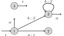
Figure 2: A monoidal transducer $\mathcal{B}$

To apply the framework of Section 2 we first need to model monoidal transducers as functors. We thus design a tailored output category that in particular matches the one for classical transducers when $M$ is a free monoid [PC20, Section 4]. We write $\mathcal{T}_{M}$ for the monad on $\mathbf{Set}$ given by $\mathcal{T}_{M}X=M\times X+1=(M\times X)\sqcup\{\bot\}$ (in Haskell, this monad is the composite of the Maybe monad and a Writer monad). Its unit $\eta:\operatorname{Id}\Rightarrow\mathcal{T}_{M}$ is given by $\eta_{X}(x)=(\epsilon,x)$ and its multiplication $\mu:\mathcal{T}_{M}^{2}\Rightarrow\mathcal{T}_{M}$ is given by $\mu_{X}((\upsilon,(\nu,x)))=(\nu\upsilon,x)$, $\mu_{X}((\upsilon,\bot))=\bot$ and $\mu_{X}(\bot)=\bot$. Recall that the Kleisli category $\mathbf{Kl}(\mathcal{T}_{M})$ for the monad $\mathcal{T}_{M}$ has sets for objects and arrows $X\mathrel{\leavevmode\hbox to22.32pt{\vbox to5.54pt{\text{[drawing]}}}}Y$ (notice the different symbol) those functions $f^{\dagger}:\mathcal{T}_{M}X\rightarrow\mathcal{T}_{M}Y$ such that $f^{\dagger}(\bot)=\bot$, $f^{\dagger}(\upsilon,x)=(\upsilon\nu,y)$ when $f^{\dagger}(\epsilon,x)=(\nu,y)$ and $f^{\dagger}(\upsilon,x)=\bot$ when $f(\epsilon,x)=\bot$: in particular, such an arrow is entirely determined by its restriction $f:X\rightarrow\mathcal{T}_{M}Y$, and we will freely switch between these two points of view for the sake of conciseness. The identity on $X$ is then given by the identity function $\operatorname{id}_{\mathcal{T}_{M}X}=\eta_{X}^{\dagger}:\mathcal{T}_{M}X\rightarrow\mathcal{T}_{M}X$, and the composition of two arrows $X\mathrel{\leavevmode\hbox to20.39pt{\vbox to5.54pt{\text{[drawing]}}}}Y\mathrel{\leavevmode\hbox to20.39pt{\vbox to5.54pt{\text{[drawing]}}}}Z$ is given by the composition of the underlying functions $\mathcal{T}_{M}X\rightarrow\mathcal{T}_{M}Y\rightarrow\mathcal{T}_{M}Z$.

$M$-transducers are in one-to-one correspondance with $(\mathbf{Kl}(\mathcal{T}_{M}),1,1)$-automata, i.e. functors $\mathcal{A}:\mathcal{I}\rightarrow\mathbf{Kl}(\mathcal{T}_{M})$ such that $\mathcal{A}(\mathtt{in})=\mathcal{A}(\mathtt{out})=1$: $(S,(\upsilon_{0},s_{0}),t,(-\odot a)_{a\in A})$ is modelled by the functor $\mathcal{A}:\mathcal{I}\rightarrow\mathbf{Kl}(\mathcal{T}_{M})$ given by $\mathcal{A}(\mathtt{st})=S$, $\mathcal{A}(\triangleright)=*\mapsto(\upsilon_{0},s_{0}):1\rightarrow M\times S+1$, $\mathcal{A}(w)=s\mapsto s\odot w=(((s\odot a_{1})\odot^{\dagger}a_{2})\odot^{\dagger}\cdots)\odot^{\dagger}a_{n}:S\rightarrow M\times S+1$ for $w=a_{1}\cdots a_{n}\in A^{*}$, and $\mathcal{A}(\triangleleft)=t:S\rightarrow M+1\cong M\times 1+1$.

We write $\mathbf{Trans}_{M}$ for the category of $(\mathbf{Kl}(\mathcal{T}_{M}),1,1)$-automata: the objects are $M$-transducers seen as functors and the morphisms are natural transformations between them. Given a $(\mathbf{Kl}(\mathcal{T}_{M}),1,1)$-language $\mathcal{L}:\mathcal{O}\rightarrow\mathbf{Kl}(\mathcal{T}_{M})$, we write $\mathbf{Trans}_{M}(\mathcal{L})$ for the subcategory of $M$-transducers $\mathcal{A}:\mathcal{I}\rightarrow\mathbf{Kl}(\mathcal{T}_{M})$ that recognize $\mathcal{L}$, i.e. such that $\mathcal{A}\circ\iota=\mathcal{L}$.

Under this correspondance, the language recognized by a transducer $(S,(\upsilon_{0},s_{0}),t,\odot)$ is thus a function $L:A^{*}\rightarrow M+1$ given by $L(w)=t^{\dagger}((\upsilon_{0},s_{0})\odot^{\dagger}w)$, and a morphism between two transducers $(S_{1},(\upsilon_{1},s_{1}),t_{1},{\odot_{1}})$ and $(S_{2},(\upsilon_{2},s_{2}),t_{2},{\odot_{2}})$ is a function $f:S_{1}\rightarrow M\times S_{2}+1$ such that $f^{\dagger}(\upsilon_{1},s_{1})=(\upsilon_{2},s_{2})$, $t_{1}(s)=t_{2}^{\dagger}(f(s))$ and $f^{\dagger}(s\odot a)=f^{\dagger}(s)\odot^{\dagger}a$.

When $M=B^{*}$ for some alphabet $B$, $M$-transducers coincide with the classical notion of transducers and the minimal transducer is given by Lemma 2 [Cho03, PC20]. To study the notion of minimal monoidal transducer, it is thus natural to try to follow this framework as well.

3.3 The initial and final monoidal transducers recognizing a function

To apply the framework of Section 2 to $(\mathbf{Kl}(\mathcal{T}_{M}),1,1)$-automata, we need three ingredients in $\mathbf{Kl}(\mathcal{T}_{M})$: countable copowers of $1$, countable powers of $1$, and a factorization system.

We start with the first ingredient, countable copowers of $1$. Since $\mathbf{Set}$ has arbitrary coproducts, $\mathbf{Kl}(\mathcal{T}_{M})$ has arbitrary coproducts as well as any Kleisli category for a monad over a category with coproducts does [Szi83, Proposition 2.2]. Hence Theorem 4 applies:

Corollary 8 (initial transducer).

For any $(\mathbf{Kl}(\mathcal{T}_{M}),1,1)$-language $\mathcal{L}$, $\mathbf{Trans}_{M}(\mathcal{L})$ has an initial object $\mathcal{A}^{init}(\mathcal{L})$ with state-set $S^{init}=A^{*}$, initial state $s_{0}^{init}=e$, initialization value $\upsilon_{0}^{init}=\epsilon$, termination function $t^{init}(w)=\mathcal{L}(\triangleright w\triangleleft)(*)$ and transition function $w\odot^{init}a=(\epsilon,wa)$. Given any other transducer $\mathcal{A}=(S,(\upsilon_{0},s_{0}),t,{\odot})$ recognizing $\mathcal{L}$, the unique transducer morphism $f:\mathcal{A}^{init}(\mathcal{L})\Longrightarrow\mathcal{A}$ is given by the function $f:A^{*}\rightarrow M\times S+1$ such that $f(w)=\mathcal{A}(\triangleright w)(*)=(\upsilon_{0},s_{0})\odot^{\dagger}w$.

Similarly, to get a final transducer in $\mathbf{Trans}_{M}(\mathcal{L})$ for some $\mathcal{L}$, Theorem 4 tells us that it is enough for $\mathbf{Kl}(\mathcal{T}_{M})$ to have all countable powers of $1$. This is in particular what happens for classical transducers, when $M$ is a free monoid [PC20, Lemma 4.7]. Hence we study conditions on the monoid $M$ for $\mathbf{Kl}(\mathcal{T}_{M})$ to have these powers.

To this means, given a countable set $I$ we consider partial functions $\Lambda:I\rightarrow M+1$. We write $\bot^{I}$ for the nowhere defined function $i\mapsto\bot$ and $(M+1)_{*}^{I}=(M+1)^{I}-\{\bot^{I}\}$ for the set of partial functions that are defined somewhere. If $I\subseteq J$, $(M+1)_{*}^{I}$ may thus be identified with the subset of partial functions of $(M+1)_{*}^{J}$ that are undefined on $J-I$. We extend the product ${\otimes}:M^{2}\rightarrow M$ of $M$ to a function $M\times(M+1)_{*}^{I}\rightarrow(M+1)_{*}^{I}$ by setting $(\upsilon\otimes\Lambda)(i)=\upsilon\otimes\Lambda(i)$ for $i\in I$ such that $\Lambda(i)\neq\bot$ and $(\upsilon\otimes\Lambda)(i)=\bot$ otherwise.The universal property of the product then translates as:

Proposition 9.

The following are equivalent:

1. [label=(0), series=countable_products_lgcd_red]

2. $\mathbf{Kl}(\mathcal{T}_{M})$ has all countable powers of $1$;

3. there are two functions $\operatorname{lgcd}:(M+1)_{*}^{\mathbb{N}}\rightarrow M$ and $\operatorname{red}:(M+1)_{*}^{\mathbb{N}}\rightarrow(M+1)_{*}^{\mathbb{N}}$ such that

   1. for all $\Lambda\in(M+1)_{*}^{\mathbb{N}}$, $\Lambda=\operatorname{lgcd}(\Lambda)\operatorname{red}(\Lambda)$;

   2. for all $\Gamma,\Lambda\in(M+1)_{*}^{\mathbb{N}}$ and $\upsilon,\nu\in M$, if $\upsilon\operatorname{red}(\Gamma)=\nu\operatorname{red}(\Lambda)$ then $\upsilon=\nu$ and $\operatorname{red}\Gamma=\operatorname{red}\Lambda$;

4. $\mathbf{Kl}(\mathcal{T}_{M})$ has all countable products.

Moreover when these hold, since any countable set $I$ embeds into $\mathbb{N}$, $\operatorname{lgcd}$ and $\operatorname{red}$ can be extended to $(M+1)_{*}^{I}$. $\operatorname{lgcd}\Lambda$ is then a left-gcd of $(\Lambda(i))_{i\mid\Lambda(i)\neq\bot}$ and the product of $(X_{i})_{i\in I}$ for some $I\subseteq\mathbb{N}$ is the set of pairs $(\Lambda,(x_{i})_{i\in I})$ such that $\Lambda\in\operatorname{red}((M+1)_{*}^{I})$ and, for all $i\in I$, $x_{i}\in X_{i}$ if $\Lambda(i)\neq\bot$ and $x_{i}=\bot$ otherwise. In particular, the $I$-th power of $1$ is the set of irreducible partial functions $I\rightarrow M+1$:

$$\prod_{I}1=\operatorname{Irr}(I,M)=\{\operatorname{red}\Lambda\in(M+1)_{*}^{I}\mid\Lambda\in(M+1)_{*}^{I}\}$$

Proof 3.3.

$\ref{prop:countable_products_lgcd_red:item:products}\Rightarrow\ref{prop:countable_products_lgcd_red:item:powers_1}$ holds by definition.

Let us now show $\ref{prop:countable_products_lgcd_red:item:powers_1}\Rightarrow\ref{prop:countable_products_lgcd_red:item:lgcd_red}$. If $\Pi_{\mathbb{N}}1$ exists, then for any $\Lambda\in(M+1)_{*}^{\mathbb{N}}$ the cone $(\Lambda(n):1\rightarrow M+1)_{n\in\mathbb{N}}$ factors through some $h:1\rightarrow\Pi_{\mathbb{N}}$ given by some $h(*)=(\delta,x_{\Lambda})$, as if $h(*)=\bot$ then $\Lambda=\bot^{\mathbb{N}}$. We thus set $\operatorname{lgcd}\Lambda=\delta$ and $\operatorname{red}(\Lambda)(n)=\pi_{n}(x_{\Lambda})$ for all $n\in\mathbb{N}$, so that in particular $\operatorname{red}(\Lambda)\neq\bot^{\mathbb{N}}$. Since $\Lambda(n)=\pi_{n}\circ h$ for all $n\in\mathbb{N}$ we get that $\Lambda=\operatorname{lgcd}(\Lambda)\operatorname{red}(\Lambda)$, and if $\Xi=\upsilon\operatorname{red}(\Gamma)=\nu\operatorname{red}(\Lambda)$, then $(*\mapsto\Xi(n))_{n\in\mathbb{N}}$ factors through both $g(*)=(\upsilon,x_{\Gamma})$ and $h(*)=(\nu,x_{\Lambda})$: $g=h$ hence $u=v$ and $\operatorname{red}\Gamma=\operatorname{red}\Lambda$. $\operatorname{lgcd}$ and $\operatorname{red}$ thus satisfy conditions 2a and 2b.

In particular when these conditions are satisfied $\operatorname{lgcd}(\Lambda)\operatorname{red}(\Lambda)=\Lambda$ hence $\operatorname{lgcd}\Lambda$ left-divides $(\Lambda(i))_{i\mid\Lambda(i)\neq\bot}$ and if $\delta$ left-divides this family then $\Lambda=\delta\Gamma$ for some $\Gamma\neq\bot^{\mathbb{N}}$ hence $\Lambda=(\delta\operatorname{lgcd}(\Gamma))\operatorname{red}(\Gamma)$ and thus $\delta$ left-divides $\operatorname{lgcd}(\Lambda)=\delta\operatorname{lgcd}(\Gamma)$.

Finally, let us show $\ref{prop:countable_products_lgcd_red:item:lgcd_red}\Rightarrow\ref{prop:countable_products_lgcd_red:item:products}$ along with the formula for the product of a countable number of objects. Given $(X_{i})_{i\in I}$ indexed by some $I\subseteq\mathbb{N}$, define $\prod_{I}X_{i}$ as in the statement of the proposition and the projection $\pi_{j}:\prod_{I}X_{i}\mathrel{\leavevmode\hbox to20.39pt{\vbox to5.54pt{\text{[drawing]}}}}X_{j}$ by $\pi_{j}(\Lambda,(x_{i})_{i\in I})=(\Lambda(j),x_{j})$ if $\Lambda(j)\neq\bot$ and $\pi_{j}(\Lambda,(x_{i})_{i\in I})=\bot$ otherwise. Given a cone $(f_{i}:1\mathrel{\leavevmode\hbox to20.39pt{\vbox to5.54pt{\text{[drawing]}}}}X_{i})$ and some $i\in I$, write $f_{i}(*)=(\Lambda(i),x_{i})$ when $f_{i}\neq\bot$ and $\Lambda(i)=x_{i}=\bot$ otherwise. Define now $h:1\mathrel{\leavevmode\hbox to20.39pt{\vbox to5.54pt{\text{[drawing]}}}}\prod_{I}X_{i}$ by $h(*)=(\operatorname{lgcd}\Lambda,(\operatorname{red}\Lambda,(x_{i})_{i\in I}))$ if $\Lambda\neq\bot^{\mathbb{N}}$ and $h(*)=\bot$ otherwise. We immediately have that $f_{i}=\pi_{i}\circ h$ by condition 2a, and that $h$ is the only such function by condition 2b.

We also write $\operatorname{lgcd}(\bot^{\mathbb{N}})=\bot$, $\operatorname{red}(\bot^{\mathbb{N}})=\bot^{\mathbb{N}}=\bot$ and do not distinguish between $(\bot,\bot)$ and $\bot$. Also note that:

Lemma 10.

Conditions 2a and 2b are equivalent to saying that

1. [label=(0), resume=countable_products_lgcd_red]

2. 1. $\langle\operatorname{lgcd},\operatorname{red}\rangle$ is injective;

   2. for all $\Lambda\in(M+1)_{*}^{\mathbb{N}}$, $\operatorname{lgcd}(\operatorname{red}\Lambda)=\epsilon$ and $\operatorname{red}(\operatorname{red}\Lambda)=\operatorname{red}\Lambda$;

   3. for all $\Lambda\in(M+1)_{*}^{\mathbb{N}}$ and $\upsilon\in M$, $\operatorname{lgcd}(\upsilon\Lambda)=\upsilon\operatorname{lgcd}(\Lambda)$ and $\operatorname{red}(\upsilon\Lambda)=\operatorname{red}(\Lambda)$.

Proof 3.4.

Assuming conditions 2a and 2b, we get that

• 1a: if $\operatorname{lgcd}\Gamma=\operatorname{lgcd}\Lambda$ and $\operatorname{red}\Gamma=\operatorname{red}\Lambda$ then

  $$\Gamma=\operatorname{lgcd}(\Gamma)\operatorname{red}(\Gamma)=\operatorname{lgcd}(\Lambda)\operatorname{red}(\Lambda)=\Lambda$$

• 1b: $\operatorname{red}\Lambda=\operatorname{lgcd}(\operatorname{red}\Lambda)\operatorname{red}(\operatorname{red}\Lambda)$ hence $\operatorname{lgcd}(\operatorname{red}\Lambda)=\epsilon$ and $\operatorname{red}(\operatorname{red}\Lambda)=\operatorname{red}\Lambda$;

• 1c: $(\upsilon\operatorname{lgcd}(\Lambda))\operatorname{red}(\Lambda)=\upsilon\Lambda$ hence $\upsilon\operatorname{lgcd}(\Lambda)=\operatorname{lgcd}(\upsilon\Lambda)$ and $\operatorname{red}(u\Lambda)=\operatorname{red}\Lambda$.

And conversely, assuming conditions 1a, 1b and 1c, we get that

• 2a: by injectivity, $\Lambda=\operatorname{lgcd}(\Lambda)\operatorname{red}(\Lambda)$ since

  $$\operatorname{lgcd}(\operatorname{lgcd}(\Lambda)\operatorname{red}(\Lambda))=\operatorname{lgcd}(\Lambda)\operatorname{lgcd}(\operatorname{red}\Lambda)=\operatorname{lgcd}\Lambda$$

  and

  $$\operatorname{red}(\operatorname{lgcd}(\Lambda)\operatorname{red}(\Lambda))=\operatorname{red}(\operatorname{red}\Lambda)=\operatorname{red}\Lambda$$

• 2b: if $\upsilon\operatorname{red}(\Gamma)=\nu\operatorname{red}(\Lambda)$ then

  $$\upsilon=\upsilon\operatorname{lgcd}(\operatorname{red}\Gamma)=\operatorname{lgcd}(\upsilon\operatorname{red}(\Gamma))=\operatorname{lgcd}(\nu\operatorname{red}(\Lambda))=\nu\operatorname{lgcd}(\operatorname{red}\Lambda)=\nu$$

  and

  $$\operatorname{red}\Gamma=\operatorname{red}(\operatorname{red}\Gamma)=\operatorname{red}(\upsilon\operatorname{red}(\Gamma))=\operatorname{red}(\nu\operatorname{red}(\Lambda))=\operatorname{red}(\operatorname{red}\Lambda)=\operatorname{red}\Lambda$$

Corollary 11.

When the functions $\operatorname{lgcd}$ and $\operatorname{red}$ exist, the final transducer $\mathcal{A}^{final}(\mathcal{L})$ recognizing a $(\mathbf{Kl}(\mathcal{T}_{M}),1,1)$-language $\mathcal{L}$ exists and has state-set $S^{final}=\operatorname{Irr}(A^{*},M)$, initial state $s_{0}^{final}=\operatorname{red}\mathcal{L}$, initialization value $\upsilon_{0}^{final}=\operatorname{lgcd}\mathcal{L}$, termination function $t^{final}(\Lambda)=\Lambda(e)$ and transition function $\Lambda\odot^{final}a=(\operatorname{lgcd}({a}^{-1}\Lambda),\operatorname{red}({a}^{-1}\Lambda))$ where we write $({a}^{-1}\Lambda)(w)=\Lambda(aw)$ for $a\in A$. Given any other transducer $\mathcal{A}=(S,(\upsilon_{0},s_{0}),t,{\odot})$ recognizing $\mathcal{L}$, the unique transducer morphism $f:\mathcal{A}\Longrightarrow\mathcal{A}^{final}(\mathcal{L})$ is given by the function $f:S\rightarrow M\times\operatorname{Irr}(A^{*},M)+1$ such that $f(s)=(\operatorname{lgcd}\mathcal{L}_{s},\operatorname{red}\mathcal{L}_{s})$ where $\mathcal{L}_{s}(\triangleright w\triangleleft)(*)=\mathcal{A}(w\triangleleft)(s)$ is the function recognized by $\mathcal{A}$ from the state $s$.

In practice we will assume that $M$ is right-noetherian to ensure algorithms terminate. It is thus interesting to see what the existence of the powers of $1$ implies in this specific case (and in particular, by Lemma 7, when $M$ is such that all right- and left-invertibles are invertibles).

Lemma 12.

If right- and left-invertibles of $M$ are all invertibles and if $\mathbf{Kl}(\mathcal{T}_{M})$ has all countable powers of $1$ then $M$ is both left-cancellative up to invertibles on the left and right-coprime-cancellative, and all non-empty countable families of $M$ have a unique left-gcd up to invertibles on the right.

Proof 3.5.

Let us first show left-cancellativity up to invertibles. If $\upsilon\gamma_{i}=\upsilon\lambda_{i}$ for some $\upsilon\in M$ and two countable families $(\gamma_{i})_{i\in I},(\lambda_{i})_{i\in I}$ of elements of $M$ with $I\subseteq\mathbb{N}_{>0}$, then defining $\Gamma(0)=\Lambda(0)=\epsilon$, $\Gamma(i)=\gamma_{i}$ and $\Lambda(i)=\lambda_{i}$ for all $i\in I$ and $\Gamma(j)=\Lambda(j)=\bot$ for all $j\notin I$, we have that $\upsilon\Gamma=\upsilon\Lambda$. Hence $\operatorname{red}\Gamma=\operatorname{red}\Lambda$ and $\upsilon\operatorname{lgcd}(\Gamma)=\upsilon\operatorname{lgcd}(\Lambda)$. But $\operatorname{lgcd}\Gamma$ and $\operatorname{lgcd}\Lambda$ left-divide $\epsilon=\Gamma(0)=\Lambda(0)$ hence they are right-invertible and thus invertible: $\gamma_{i}$ and $\lambda_{i}=\operatorname{lgcd}(\Lambda){\operatorname{lgcd}(\Gamma)}^{-1}\gamma_{i}$ are equal up to an invertible (that does not depend on $i$) on the left.

Moreover, if $\upsilon\Lambda=\nu\Lambda$ for some $\Lambda$ such that $(\Lambda(i))_{i\mid\Lambda(i)\neq\bot}$ is left-coprime, then $\operatorname{lgcd}\Lambda$ is right-invertible (by definition of left-coprimality) and since

$$\upsilon\operatorname{lgcd}(\Lambda)=\operatorname{lgcd}(\upsilon\Lambda)=\operatorname{lgcd}(\nu\Lambda)=\nu\operatorname{lgcd}(\Lambda)$$

we get by left-invertibility of $\operatorname{lgcd}\Lambda$ that $\upsilon=\nu$.

Finally, consider $\delta$ a left-gcd of some non-empty countable family encoded as $\Lambda\in(M+1)_{*}^{\mathbb{N}}$. Then there is some $\upsilon$ such that $\delta=\operatorname{lgcd}(\Lambda)\upsilon$ (since $\operatorname{lgcd}(\Lambda)$ left-divides $\Lambda$) and some $\Gamma$ such that $\delta\Gamma=\Lambda$. Hence

$$\operatorname{lgcd}\Lambda=\operatorname{lgcd}(\delta\Gamma)=\delta\operatorname{lgcd}(\Gamma)=\operatorname{lgcd}(\Lambda)\upsilon\operatorname{lgcd}(\Gamma)$$

By left-cancellativity up to invertibles, $\upsilon\operatorname{lgcd}(\Gamma)\in{M}^{\times}$ so $\upsilon$ is right-invertible hence invertible: $\delta=\operatorname{lgcd}\Lambda$ up to invertibles on the right.

And conversely, these conditions on $M$ are enough for $\mathbf{Kl}(\mathcal{T}_{M})$ to have all countable powers of $1$ (even when $M$ is not noetherian), while being easier to show than properly defining the two functions $\operatorname{lgcd}$ and $\operatorname{red}$.

Lemma 13.

If $M$ is both left-cancellative up to invertibles on the left and right-coprime-cancellative, and all non-empty countable subsets of $M$ have a unique left-gcd up to invertibles on the right, then $\mathbf{Kl}(\mathcal{T}_{M})$ has all countable powers of $1$.

Proof 3.6.

Split the set of those $\Lambda\in(M+1)_{*}^{\mathbb{N}}$ such that $(\Lambda(i))_{i\mid\Lambda(i)\neq\bot}$ is left-coprime into the equivalence classes given by $\chi\Lambda\sim\Lambda$ for all $\chi\in{M}^{\times}$. Then, for each equivalence class $C$ pick a $\operatorname{red}C$ in $C$ (using the axiom of choice) and for all $\upsilon\in M$ define $\operatorname{lgcd}(\upsilon\operatorname{red}(C))=\upsilon$ and $\operatorname{red}(\upsilon\operatorname{red}(C))=\operatorname{red}C$ so that in particular $\operatorname{lgcd}(\operatorname{red}C)=\epsilon$ and $\operatorname{red}(\operatorname{red}C)=\operatorname{red}C$.

This is well-defined because if $\upsilon\operatorname{red}(C)=\nu\operatorname{red}(D)$ for $\upsilon,\nu\in M$ and two equivalence classes $C,D$, then if $\delta$ is a left-gcd of $\upsilon\operatorname{red}(C)$ we have that $\delta=\upsilon\upsilon^{\prime}$ for some $\upsilon^{\prime}$ (since $\upsilon$ left-divides $\upsilon\operatorname{red}(C)$) and there is some $\Lambda$ such that $\upsilon\operatorname{red}(C)=\upsilon\upsilon^{\prime}\Lambda$. But then by left-cancellativity up to invertibles, there is some $\chi\in{M}^{\times}$ such that $\upsilon^{\prime}\Lambda=\chi\operatorname{red}(C)$, hence ${\chi}^{-1}\upsilon^{\prime}$ left-divides $\operatorname{red}C$ and as such is right-invertible (it left-divides $\epsilon$, a left-gcd of $\operatorname{red}C$), making $\upsilon^{\prime}$ right-invertible as well. This shows that $\upsilon$ is a left-gcd of $\upsilon\operatorname{red}(C)=\nu\operatorname{red}(D)$ and we show similarly that this is also true of $\nu$, hence by unicity of the left-gcd there is a $\xi\in{M}^{\times}$ such that $\upsilon=\nu\xi$. Therefore by left-cancellativity up to invertibles there is another invertible $\xi^{\prime}\in{M}^{\times}$ such that $\xi\operatorname{red}(C)=\xi^{\prime}\operatorname{red}(D)$ hence by definition $C=D$ and, by right-coprime-cancellativity, $\upsilon=\nu$.

Moreover this defines $\operatorname{lgcd}\Lambda$ and $\operatorname{red}\Lambda$ for any $\Lambda$ because if $\delta$ is a left-gcd of $\Lambda$, then $\Lambda=\delta\Gamma$ for some left-coprime $\Gamma$ (if $\delta^{\prime}$ left-divides $\Gamma$ then $\delta\delta^{\prime}$ left-divides $\Lambda$ hence $\delta$, therefore $\delta^{\prime}$ is invertible by left-cancellativity up to invertibles) hence $\Lambda=\delta\chi\operatorname{red}(C)$ if $\Gamma\in C$ and $\Gamma=\chi\operatorname{red}(C)$.

We have thus defined two functions $\operatorname{lgcd}$ and $\operatorname{red}$ that immediately satisfy the conditions 2a and 2b of Proposition 9.

When $M$ is a group it is cancellative (because all elements are invertible) and all countable families have a unique left-gcd up to invertibles on the right ($\epsilon$ itself) hence Lemma 13 applies and $\mathbf{Trans}_{M}(\mathcal{L})$ always has a final object.

The same is true when $M$ is a trace monoid (the left-gcd then being the longest common prefix, whose existence is guaranteed by [CP85, Proposition 1.3]).

Conversely, the monoids given by join semi-lattices are not left-cancellative up to invertibles in general. In $\mathbb{R}_{+}$ for instance, there are ways to define the functions $\operatorname{lgcd}$ and $\operatorname{red}$ but they may not satisfy condition 1c, more precisely that $\operatorname{red}(\upsilon\Lambda)=\operatorname{red}\Lambda$. This is expected, as there may be several non-isomorphic ways to minimize automata with outputs in these monoids, which is incompatible with the framework of Lemma 2.

Lemma 13 provides sufficient conditions that are reminiscent of those developed in [Ger18] for the minimization of monoidal transducers. These conditions are stronger than ours but still similar: the output monoid is assumed to be both left- and right-cancellative, which in particular implies the unicity up to invertibles on the right of the left-gcd whose existence is also assumed. They do only require the existence of left-gcds for finite families (whereas we ask for left-gcds of countable families), which would not be enough for our sake since the categorical framework also encompasses the existence of minimal (infinite) automata for non-regular languages, but in practice our algorithms will only use binary left-gcds as well. We conjecture that, when only those binary left-gcds exist, the existence of a unique minimal transducer is explained categorically by the existence of a final transducer in the category of transducers whose states all recognize functions that are themselves recognized by finite transducers. Where the two sets of conditions really differ is in the conditions required for the termination of the algorithms: where we will require right-noetherianity of $M$, they require that if some $\nu$ left-divides both some $\omega$ and $\upsilon\omega$ for some $\upsilon$, then $\nu$ should also left-divide $\upsilon\nu$. This last condition leads to better complexity bounds than right-noetherianity, but misses some otherwise simple monoids that satisfy right-noetherianity, e.g. $\{\alpha,\beta\}^{*}$ but where we also let $\alpha$ and $\beta^{2}$ commute. Conversely, Gerdjikov’s main non-trivial example, the tropical monoid $(\mathbb{R}_{+},0,+)$, is not right-noetherian. It can still be dealt with in our context by considering submonoids (finitely) generated by the output values of a finite transducer’s transitions, these monoids themselves being right-noetherian.

3.4 Factorization systems

The last ingredient we need in order to be able to apply the framework of Section 2 is a factorization system on $\mathbf{Trans}_{M}(\mathcal{L})$. By Lemma 2, it is enough to find a factorization system on $\mathbf{Kl}(\mathcal{T}_{M})$.

When $M$ is a free monoid, define $\mathcal{E}=\mathrm{Surj}$ to be the class of those functions $f:X\rightarrow M\times Y+1$ that are surjective on $Y$ and $\mathcal{M}=\mathrm{Inj}\cap\mathrm{Eps}\cap\mathrm{Tot}$ to be the class of those functions $f:X\rightarrow M\times Y+1$ that are total ($f\in\mathrm{Tot}$), injective when corestricted to $Y$ ($f\in\mathrm{Inj}$), and only produce the empty word ($f\in\mathrm{Eps}$). Then the $(\mathcal{E},\mathcal{M})$-minimal transducer recognizing a function is the one defined by Choffrut [Cho03, PC20]: in particular, the fact that the minimal transducer $(\mathcal{E},\mathcal{M})$-divides all other transducers means (thanks to the surjectivity of $\mathcal{E}$-morphisms and the injectivity of $\mathcal{M}$-morphisms) that it has the smallest possible state-set and produces its outputs as early as possible.

It is thus natural to try and extend this factorization system to $\mathbf{Kl}(\mathcal{T}_{M})$ for arbitrary $M$. It is not enough by itself because isomorphisms may produce invertible elements that may be different from $\epsilon$: $\mathrm{Iso}\subsetneq\mathrm{Surj}\cap\mathrm{Inj}\cap\mathrm{Eps}\cap\mathrm{Tot}$, yet we need the intersection $\mathcal{E}\cap\mathcal{M}$ to be $\mathrm{Iso}$. $\mathcal{M}$-morphisms must thus be able to produce invertible elements as well. Formally, define therefore $\mathrm{Surj}$, $\mathrm{Inj}$, $\mathrm{Tot}$ and $\mathrm{Inv}$ as follows. For $f:X\rightarrow M\times Y+1$, write $f_{1}:X\rightarrow M+1$ for its projection on $M$ and $f_{2}:X\rightarrow Y+1$ for its projection on $Y$: we let $f\in\mathrm{Surj}$ whenever $f_{2}$ is surjective on $Y$, $f\in\mathrm{Inj}$ whenever $f_{2}$ is injective when corestricted to $Y$, $f\in\mathrm{Tot}$ whenever $f(x)\neq\bot$ for all $x\in X$ and $f\in\mathrm{Inv}$ whenever $f_{1}(x)$ is either $\bot$ or in ${M}^{\times}$. The point is that when replacing $\mathrm{Eps}$ with $\mathrm{Inv}$, we get back that

Lemma 14.

In $\mathbf{Kl}(\mathcal{T}_{M})$, $\mathrm{Iso}=\mathrm{Surj}\cap\mathrm{Inj}\cap\mathrm{Inv}\cap\mathrm{Tot}$, and these four classes are all closed under composition (within themselves).

Proof 3.7.

Closure under composition is immediate.

If $f:X\rightarrow M\times Y+1$ is in $\mathrm{Surj}\cap\mathrm{Inj}\cap\mathrm{Inv}\cap\mathrm{Tot}$, it can be restricted to a function $\langle f_{1},f_{2}\rangle:X\rightarrow M\times Y$ ($f\in\mathrm{Tot}$). $f_{2}$ must be bijective ($f\in\mathrm{Surj}\cap\mathrm{Inj}$) and $f_{1}(X)\subseteq{M}^{\times}$ ($f\in\mathrm{Inv}$). Hence $f$ has an inverse, given by $({f}^{-1})(y)=\left(({f_{1}({f_{2}}^{-1}(y))}^{-1},{f_{2}}^{-1}(y)\right)$.

Conversely, if $f:X\rightarrow M\times Y+1$ is an isomorphism it has an inverse ${f}^{-1}:Y\rightarrow M\times X+1$ such that $f\circ{f}^{-1}=\operatorname{id}_{Y}$ and ${f}^{-1}\circ f=\operatorname{id}_{X}$. For all $x\in X$, $({f}^{-1})^{\dagger}(f(x))=(\epsilon,x)$ hence $f(x)\neq\bot$: $f\in\mathrm{Tot}$, and similarly for ${f}^{-1}$. Writing $f=\langle f_{1},f_{2}\rangle$ and ${f}^{-1}=\langle({f}^{-1})_{1},({f}^{-1})_{2}\rangle$, we have that $f_{2}$ is a bijection with inverse ${f_{2}}^{-1}=({f}^{-1})_{2}$, hence $f\in\mathrm{Surj}\cap\mathrm{Inj}$. Finally, for all $x\in X$ we have that $f_{1}(x)({f}^{-1})_{1}(f_{2}(x))=\epsilon$ and conversely, hence $f_{1}(x)$ is invertible and $f\in\mathrm{Inv}$.

The different ways in which we may distribute these four classes into the two classes $\mathcal{E}$ and $\mathcal{M}$ leads to not just one but three interesting factorization systems:

Proposition 15.

$(\mathcal{E}_{1},\mathcal{M}_{1})=(\mathrm{Surj}\cap\mathrm{Inj}\cap\mathrm{Inv},\mathrm{Tot})$, $(\mathcal{E}_{2},\mathcal{M}_{2})=(\mathrm{Surj}\cap\mathrm{Inj},\mathrm{Inv}\cap\mathrm{Tot})$ and $(\mathcal{E}_{3},M_{3})=(\mathrm{Surj},\mathrm{Inj}\cap\mathrm{Inv}\cap\mathrm{Tot})$ are all factorization systems in $\mathbf{Kl}(\mathcal{T}_{M})$.

Proof 3.8.

By Lemma 14 we only need to show for each $i\in\{1,2,3\}$ that every $f:X\mathrel{\leavevmode\hbox to20.39pt{\vbox to5.54pt{\text{[drawing]}}}}Y$ may be factored as $m\circ e$ with $e\in\mathcal{E}_{i}$ and $m\in\mathcal{M}_{i}$, and that $\mathcal{E}_{i}$ and $\mathcal{M}_{i}$ satisfy the diagonal fill-in property of Section 2.2.

• $(\mathcal{E}_{1},\mathcal{M}_{1})$. Any $f:X\rightarrow M\times Y+1$ may be factored through $e:X\rightarrow M\times f^{-1}(M\times Y)+1$ (given by $e(x)=(\epsilon,x)$ if $e(x)\neq\bot$ and $e(x)=\bot$ otherwise) and $m:f^{-1}(M\times Y)\rightarrow M\times Y+1$ (given by $m(x)=e(x)$ when $e(x)\neq\bot$).

  Moreover, given a commuting diagram

  the only possible choice for a $\phi:Y_{1}\rightarrow M\times Y_{2}+1$ is given by $\phi(y_{1})=\bot$ if $v(y_{1})=\bot$ and $\phi(y_{1})=({\upsilon_{e}}^{-1}\upsilon_{u},y_{2})$ if $e(x)=(\upsilon_{e},y_{1})$, $u(x)=(\upsilon_{u},y_{2})$, $v(y_{1})=(\upsilon_{v},z)$, $m(y_{2})=(\upsilon_{m},z)$ and $\upsilon_{e}\upsilon_{v}=\upsilon_{u}\upsilon_{m}$. This definition does not depend on the choice of $x$ because of the bijectiveness property of $e$, and we immediately have the commuting diagram

  by definition.

• $(\mathcal{E}_{2},\mathcal{M}_{2})$. Any $f:X\rightarrow M\times Y+1$ may be factored through $e:X\rightarrow M\times f^{-1}(M\times Y)+1$ (given by $e(x)=(\upsilon,x)$ if $e(x)=(\upsilon,\--)$ and $e(x)=\bot$ otherwise) and $m:f^{-1}(M\times Y)\rightarrow M\times Y+1$ (given by $m(x)=(\epsilon,y)$ when $e(x)=(\--,y)$).

  Finally, given a commuting diagram

  the only possible choice for a $\phi:Y_{1}\rightarrow M\times Y_{2}+1$ is given by $\phi(y_{1})=\bot$ if $v(y_{1})=\bot$ and $\phi(y_{1})=(\upsilon_{v}{\upsilon_{m}}^{-1},y_{2})$ if $e(x)=(\upsilon_{e},y_{1})$, $u(x)=(\upsilon_{u},y_{2})$, $v(y_{1})=(\upsilon_{v},z)$, $m(y_{2})=(\upsilon_{m},z)$ and $\upsilon_{e}\upsilon_{v}=\upsilon_{u}\upsilon_{m}$. This definition does not depend on the choice of $x$ because of the bijectiveness property of $e$, and we immediately have the commuting diagram

  by definition.

• $(\mathcal{E}_{3},\mathcal{M}_{3})$. Any morphism $f:X\rightarrow M\times Y+1$ factors through $e:X\rightarrow M\times Z+1$ and $m:Z\rightarrow M\times Y+1$ with

  $$Z=\{y\in Y\mid\exists x\in X,f(x)=(\--,y)\}$$

  $e(x)=f(x)$ and $m(y)=(\epsilon,y)$.

  Finally, given a commuting diagram

  the only possible choice for a $\phi:Y_{1}\rightarrow M\times Y_{2}+1$ is given by $\phi(y_{1})=\bot$ if $v(y_{1})=\bot$ and $\phi(y_{1})=(\upsilon_{v}{\upsilon_{m}}^{-1},y_{2})$ if $e(x)=(\upsilon_{e},y_{1})$, $u(x)=(\upsilon_{u},y_{2})$, $v(y_{1})=(\upsilon_{v},z)$, $m(y_{2})=(\upsilon_{m},z)$ and $\upsilon_{e}\upsilon_{v}=\upsilon_{u}\upsilon_{m}$. This definition does not depend on the choice of $x$ because $m$ is injective on $Y$, and we immediately have the commuting diagram

  by definition.

The factorization system we choose to define the minimal $M$-transducer is $(\mathcal{E}_{3},\mathcal{M}_{3})=(\mathrm{Surj},\mathrm{Inj}\cap\mathrm{Inv}\cap\mathrm{Tot})$, because it generalizes the factorization system that defines the minimal transducer (with output in a free monoid). It will be our main factorization system, and as such from now on we reserve the notation $(\mathcal{E},\mathcal{M})$ for it.

Theorem 4 and Proposition 3 show that $(\mathcal{E},\mathcal{M})$ indeed gives rise to a useful notion of minimal transducer.

Corollary 16.

When $\mathbf{Kl}(\mathcal{T}_{M})$ has all countable powers of $1$, the $(\mathcal{E},\mathcal{M})$-minimal transducer recognizing a $(\mathbf{Kl}(\mathcal{T}_{M}),1,1)$-language $\mathcal{L}$ is well-defined and has state-set $S^{min}=\{\operatorname{red}({w}^{-1}\mathcal{L})\mid w\in A^{*}\}\cap(M+1)_{*}^{A^{*}}$, initial state $s_{0}^{min}=\operatorname{red}\mathcal{L}$, initialization value $\upsilon_{0}^{min}=\operatorname{lgcd}\mathcal{L}$, termination function $t^{min}(\Lambda)=\Lambda(e)$ and transition functions $\operatorname{red}({w}^{-1}\mathcal{L})\odot^{min}a=(\operatorname{lgcd}({(wa)}^{-1}\mathcal{L}),\operatorname{red}({(wa)}^{-1}\mathcal{L}))$. It is characterized by the property that all its states are reachable from the initial state and recognize distinct left-coprime functions.

Why are $(\mathcal{E}_{1},\mathcal{M}_{1})$ and $(\mathcal{E}_{2},\mathcal{M}_{2})$ also interesting then ? They do not give rise to useful notions of minimality, but they show that the computation of $\operatorname{Obs}$ can be split into substeps. Indeed, since $\mathcal{E}_{1}\subset\mathcal{E}_{2}\subset\mathcal{E}_{3}$ (and equivalently $\mathcal{M}_{1}\supset\mathcal{M}_{2}\supset\mathcal{M}_{3}$), $(\mathcal{E}_{i},\mathcal{M}_{i})_{1\leq i\leq 3}$ is a quaternary factorization system:

Corollary 17.

For every $\mathbf{Kl}(\mathcal{T}_{M})$-arrow $f:X\mathrel{\leavevmode\hbox to20.39pt{\vbox to5.54pt{\text{[drawing]}}}}Y$, there is a unique (up to isomorphisms) factorization of $f$ into

such that $f_{1}\in\mathcal{E}_{1}$, $f_{2}\in\mathcal{E}_{2}\cap\mathcal{M}_{1}$, $f_{3}\in\mathcal{E}_{3}\cap\mathcal{M}_{2}$ and $f_{4}\in\mathcal{M}_{3}$.

Note how we respectively write $\mathrel{\leavevmode\hbox to24.74pt{\vbox to12.89pt{\text{[drawing]}}}}$, $\mathrel{\leavevmode\hbox to24.74pt{\vbox to12.89pt{\text{[drawing]}}}}$, $\mathrel{\leavevmode\hbox to24.74pt{\vbox to12.89pt{\text{[drawing]}}}}$ and $\mathrel{\leavevmode\hbox to24.74pt{\vbox to12.89pt{\text{[drawing]}}}}$ for arrows in $\mathcal{E}_{1}$, $\mathcal{E}_{2}$, $\mathcal{M}_{1}$ and $\mathcal{M}_{2}$ (but stick with $\mathrel{\leavevmode\hbox to20.39pt{\vbox to5.54pt{\text{[drawing]}}}}$ and $\mathrel{\leavevmode\hbox to20.39pt{\vbox to5.54pt{\text{[drawing]}}}}$ for arrows in $\mathcal{E}=\mathcal{E}_{3}$ and $\mathcal{M}=\mathcal{M}_{3}$).

Intuitively, this results means that the computation of any $f$ can be factored into four parts: first forgetting some inputs ($f_{1}$ belongs to $\mathrm{Surj}\cap\mathrm{Inj}\cap\mathrm{Inv}$ but need not belong to $\mathrm{Tot}$), then producing non-invertible elements of the output monoid ($f_{2}$ belongs to $\mathrm{Surj}\cap\mathrm{Inj}\cap\mathrm{Tot}$ but need not belong to $\mathrm{Inv}$), then merging some inputs together ($f_{3}$ belongs to $\mathrm{Surj}\cap\mathrm{Inv}\cap\mathrm{Tot}$ but need not belong to $\mathrm{Inj}$) and finally embedding the result into a bigger set ($f_{4}$ belongs to $\mathrm{Inv}\cap\mathrm{Inj}\cap\mathrm{Tot}$ but need not belong to $\mathrm{Surj}$).

In particular, the $\mathcal{E}$-quotient $\operatorname{Reach}\mathcal{A}\mathrel{\leavevmode\hbox to20.39pt{\vbox to5.54pt{\text{[drawing]}}}}\operatorname{Obs}(\operatorname{Reach}\mathcal{A})$ factors as follows.

Given an $M$-transducer $\mathcal{A}$ recognizing the $(\mathbf{Kl}(\mathcal{T}_{M}),1,1)$-language $\mathcal{L}$, define $\operatorname{Total}\mathcal{A}$ and $\operatorname{Prefix}\mathcal{A}$ to be the $(\mathcal{E}_{1},\mathcal{M}_{1})$- and $(\mathcal{E}_{2},\mathcal{M}_{2})$-factorizations of the final arrow $\operatorname{Reach}\mathcal{A}\mathrel{\leavevmode\hbox to20.39pt{\vbox to5.54pt{\text{[drawing]}}}}\mathcal{A}^{final}(\mathcal{L})$:

In practice, if $\mathcal{A}=(S,(u_{0},s_{0}),t,{\odot})$,

• $\operatorname{Reach}\mathcal{A}$ has state-set the set of states in $S$ that are reachable from $s_{0}$;

• $\operatorname{Total}\mathcal{A}$ has state-set $S^{\prime}$ the set of states in $S$ that recognize a function defined for at least one word (in particular if $\mathcal{A}$ recognizes $\bot^{A^{*}}$ then $(u_{0},s_{0})$ is set to $\bot$);

• $\operatorname{Prefix}\mathcal{A}=(S^{\prime},(u_{0}\operatorname{lgcd}(\mathcal{L}_{s_{0}}),s_{0}),t^{\prime},{\odot^{\prime}})$, where $\mathcal{L}_{s}$ is the function recognized from a state $s\in S$ in $\mathcal{A}$, is obtained from $\operatorname{Total}\mathcal{A}$ by setting $t^{\prime}(s)={\operatorname{lgcd}(\mathcal{L}_{s})}^{-1}t(s)$ and $s\odot^{\prime}a=({\operatorname{lgcd}(\mathcal{L}_{s})}^{-1}(s\ocircle a)\operatorname{lgcd}(\mathcal{L}_{s\cdot a}),s\cdot a)$;

• $\operatorname{Min}\mathcal{L}\cong\operatorname{Obs}(\operatorname{Reach}\mathcal{A})$ is obtained from $\operatorname{Prefix}\mathcal{A}$ by merging two states $s_{1}$ and $s_{2}$ whenever they recognize functions that are equal up to invertibles on the left in $\operatorname{Prefix}\mathcal{A}$, that is when $\operatorname{red}(\mathcal{L}_{s_{1}})=\operatorname{red}(\mathcal{L}_{s_{2}})$ in $\mathcal{A}$.

In particular, these four steps (computing $\operatorname{Reach}\mathcal{A}$, $\operatorname{Total}\mathcal{A}$, $\operatorname{Prefix}\mathcal{A}$ and finally $\operatorname{Obs}\mathcal{A}$) match exactly the four steps into which all the algorithms for minimizing (possibly monoidal) transducers are decomposed [Bre98, Cho03, Eis03, Ger18, BC00].

For the transducer $\mathcal{B}$ of Figure 2 seen as a transducer with output in the free commutative monoid $\Sigma^{\oast}$, the corresponding minimal transducer $\operatorname{Min}\mathcal{L}$ is computed step-by-step in Figure 3.

Notice in particular how in Figure 3(b) both the functions recognized by the states $1$ and $3$ are left-divisible by $\alpha$ hence $\alpha$ is pulled back to the initialization value in Figure 3(c). This would not have happened had $M$ been the free monoid $\Sigma^{*}$, and the corresponding minimal transducer would have been different.

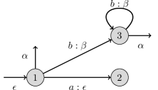
(a) $\operatorname{Reach}\mathcal{B}$

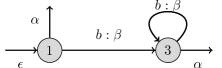
(b) $\operatorname{Total}\mathcal{B}$

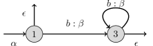
(c) $\operatorname{Prefix}\mathcal{B}$

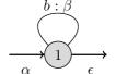
(d) $\operatorname{Obs}(\operatorname{Reach}\mathcal{B})$

Figure 3: Increasingly small transducers recognizing the same function as the transducer of Figure 2 when $M=\Sigma^{\oast}$

4 Active learning of minimal monoidal transducers

Let $M$ be a monoid satisfying the conditions of Lemma 13 and consider now a function $A^{*}\rightarrow M+1$ seen as a $(\mathbf{Kl}(\mathcal{T}_{M}),1,1)$-language $\mathcal{L}$. Theorem 4 tells us that the minimal $M$-transducer recognizing $\mathcal{L}$ exists, is unique up to isomorphism and is given by Corollary 16, but does not tell us whether this minimal transducer is computable. For this to hold we need that the product in $M$, the left-gcd of two elements in $M$ — written $\wedge$ — and the function LeftDivide — that takes as input $\delta,\upsilon\in M$ and outputs a $\nu$ such that $\upsilon=\delta\nu$ or fails if there is none — be all computable, and that equality up to invertibles on the left be decidable (and that the corresponding invertible be computable as well). We extend these operations to $M+1$ by means of $u\bot=\bot u=\bot$, $u\wedge\bot=\bot\wedge u=\bot$ and $\textsc{LeftDivide}(\delta,\bot)=\bot$. For the computations to terminate we additionally require that $\operatorname{Min}\mathcal{L}$ have finite state-set and $M$ be right-noetherian, so that $(\operatorname{Min}\mathcal{L})(\mathtt{st})$ is noetherian for the factorization system $(\mathrm{Surj},\mathrm{Inj}\cap\mathrm{Inv}\cap\mathrm{Tot})$ of Proposition 15:

Lemma 18.

An object $X$ of $\mathbf{Kl}(\mathcal{T}_{M})$ is $\mathcal{M}$-noetherian if and only if it is a finite set, in which case $\operatorname{length}_{\mathcal{M}}(m:Y\rightarrowtail X)=\left|X\right|-\left|Y\right|$.

Proof 4.1.

Let $(x_{i}:1\mathrel{\leavevmode\hbox to20.39pt{\vbox to5.54pt{\text{[drawing]}}}}X)_{i\in\mathbb{N}}$ be an infinite sequence of distincts elements of an infinite set $X$. Then the $m_{n}=[\kappa_{i}]_{i=0}^{n}:\coprod_{i=0}^{n}1\mathrel{\leavevmode\hbox to20.39pt{\vbox to5.54pt{\text{[drawing]}}}}\coprod_{i=0}^{n+1}1$ provide a counter-example to the $\mathcal{M}$-noetherianity of $X$ as none of them are isomorphisms (they are not surjective) yet $[x_{i}]_{i=0}^{n+1}\circ m_{n}=[x_{i}]_{i=0}^{n}$ and $[x_{i}]_{i=0}^{n}$ is always an $\mathcal{M}$-morphism. Hence infinite sets are never $\mathcal{M}$-noetherian. If $X$ and the sequence $(x_{i})_{i\in\mathbb{N}}$ were finite instead, this example would prove that $\operatorname{length}_{\mathcal{M}}(m:Y\rightarrowtail X)\geq\left|X\right|-\left|Y\right|$.

Conversely, a strict chain of $\mathcal{M}$-subobjects of $X$ is a strict chain of subsets $X_{0}\subsetneq X_{1}\subsetneq\cdots$ of $X$. In particular, the cardinality of these subsets is strictly increasing: if $X$ is finite, the chain must be finite as well, and its length at most $\left|X\right|-\left|X_{0}\right|$.

Lemma 19.

An object $X$ of $\mathbf{Kl}(\mathcal{T}_{M})$ is $\mathcal{E}$-artinian if and only if it is a finite set and either $M$ is right-noetherian or $X=\varnothing$, in which case $\operatorname{colength}_{\mathcal{E}}(e:X\mathrel{\leavevmode\hbox to20.39pt{\vbox to5.54pt{\text{[drawing]}}}}Y)=\left|X\right|-\left|Y\right|+\operatorname{rk}e$ where $\operatorname{rk}e=\sum_{e(x)=(\upsilon,y)}\operatorname{rk}\upsilon$.

Proof 4.2.

Let $(x_{i})_{i\in\mathbb{N}}$ be an infinite sequence of distincts elements of an infinite set $X$, and set $X_{n}=\{x_{i}\mid 0\leq i\leq n\}$. Let $e_{n}:X\mathrel{\leavevmode\hbox to20.39pt{\vbox to5.54pt{\text{[drawing]}}}}X_{n}$ be defined by $e(x_{i})=(\epsilon,x_{i})$ for $i\leq n$ and $e(x)=\bot$ otherwise, and let $e_{n}^{n+1}:X_{n+1}\mathrel{\leavevmode\hbox to20.39pt{\vbox to5.54pt{\text{[drawing]}}}}X_{n}$ be the restriction of $e_{n}$ to $X_{n+1}$. None of the $e_{n}^{n+1}$ are isomorphisms (they are not total) yet $e_{n}^{n+1}\circ e_{n+1}=e_{n}$: infinite sets are never $\mathcal{E}$-artinian.

Assume now $X$ is not empty and $M$ is not right-noetherian: there is an element $x_{*}\in X$ and two sequences $(\upsilon_{n})_{n\in\mathbb{N}}$ and $(\nu_{n})_{n\in\mathbb{N}}$ of elements of $M$ such that for all $n\in\mathbb{N}$, $\upsilon_{n}\notin{M}^{\times}$ and $\nu_{n}=\nu_{n+1}\upsilon_{n}$. Let $e_{n}:X\mathrel{\leavevmode\hbox to20.39pt{\vbox to5.54pt{\text{[drawing]}}}}1$ be defined by $e_{n}(x_{*})=(\nu_{n},*)$ and $e_{n}(x)=\bot$ for all other $x\in X$, and let $e_{n}^{n+1}:1\mathrel{\leavevmode\hbox to20.39pt{\vbox to5.54pt{\text{[drawing]}}}}1$ be defined by $e_{n}^{n+1}(*)=(\upsilon_{n},*)$. None of the $e_{n}^{n+1}$ are isomorphisms (they do not only produce invertible elements of $M$) yet $e_{n}^{n+1}\circ e_{n+1}=e_{n}$: non-empty sets are never $\mathcal{E}$-artinian when $M$ is not right-noetherian.

Conversely, if $X$ is empty then it is immediately $\mathcal{E}$-artinian: there is only one $\mathcal{E}$-morphism out of $X$, $\operatorname{id}_{X}$. Suppose now that $X$ is finite and $M$ right-noetherian, and consider a cochain $e_{n}^{n+1}:X_{n+1}\mathrel{\leavevmode\hbox to20.39pt{\vbox to5.54pt{\text{[drawing]}}}}X_{n}$ of $\mathcal{E}$-quotients $e_{n}:X\mathrel{\leavevmode\hbox to20.39pt{\vbox to5.54pt{\text{[drawing]}}}}X_{n}$. Since $X$ is finite, at most $\left|X\right|-\left|X_{0}\right|$ of the $\mathcal{E}$-quotients $X_{n+1}\mathrel{\leavevmode\hbox to20.39pt{\vbox to5.54pt{\text{[drawing]}}}}X_{n}$ witness a decrease of the cardinality from their domain to their codomain and are not in $\mathrm{Inj}\cap\mathrm{Tot}$. Fix now an $x\in X$ such that $e_{0}(x)\neq\bot$ and write $e_{n}(x)=(\nu_{n},x_{n})$ and $e_{n}^{n+1}(x_{n+1})=(\upsilon_{n},x_{n})$ (this is well-defined because $e_{n}^{n+1}\circ e_{n+1}=e_{n}$). Then $\nu_{n}=\nu_{n+1}\upsilon_{n}$ for all $n\in\mathbb{N}$, hence since $M$ is right-noetherian only a finite number of the $e_{n}^{n+1}$, at most $\operatorname{rk}\nu_{0}$, produce a non-invertible element on $x_{n+1}$. This is true for all $x\in X$, hence a finite number of the $e_{n}^{n+1}$, at most $\operatorname{rk}e_{0}$, are not in $\mathrm{Inv}$, and a finite number of them, at most $\left|X\right|-\left|X_{0}\right|+\operatorname{rk}e_{0}$, are not in $\mathrm{Iso}$: $X$ is $\mathcal{E}$-artinian and $\operatorname{colength}_{\mathcal{E}}(e_{0}:X\mathrel{\leavevmode\hbox to20.39pt{\vbox to5.54pt{\text{[drawing]}}}}X_{0})\leq\left|X\right|-\left|X_{0}\right|+\operatorname{rk}e_{0}$.

Finally, if $\operatorname{rk}e$ is finite, in light of this proof it is now easy to build a strict cochain of $\mathcal{E}$-quotients of $X$ starting with $e:X\mathrel{\leavevmode\hbox to20.39pt{\vbox to5.54pt{\text{[drawing]}}}}Y$ that has length exactly $\left|X\right|-\left|Y\right|+\operatorname{rk}e$. For each $\nu(x)\in M$ such that $e(x)=(\nu(x),y)$ for some $x\in X$ and $y\in Y$, write indeed $\upsilon_{1}(x),\ldots,\upsilon_{\operatorname{rk}\nu(x)}(x)$ for a sequence of non-invertible divisors of $\nu$ of maximum length. Each morphism between two consecutive $\mathcal{E}$-quotients in the cochain should either decrease the size of the quotient by $1$, or produce exactly one of the $\upsilon_{i}(x)$ on $x$ for exactly one $x\in X$. Similarly, if $\operatorname{rk}e$ is infinite there sequences of divisors of some $\nu(x)$ or arbitrary length and it is then easy to build strict cochains of $\mathcal{E}$-quotients of $X$ of arbitrary lengths.

The categorical framework of Section 2 can be extended with an abstract minimization algorithm [Ari23]. With the output category described in Section 3, an instance of this is in particular Gerdjikov’s algorithm for minimizing monoidal transducers [Ger18], and even shows that the latter is still valid under the conditions discussed in Section 3.3 and terminates as soon as $M$ is right-noetherian. However, we focus here on a second way to compute the minimal transducer recognizing $\mathcal{L}$, namely learning it through membership and equivalence queries, that is relying on a function $\textsc{Eval}_{\mathcal{L}}$ that outputs the value of $\mathcal{L}$ on input words and a function $\textsc{Equiv}_{\mathcal{L}}$ that checks whether the hypothesis transducer is $\operatorname{Min}\mathcal{L}$ or outputs a counterexample otherwise. Such an algorithm is an instance of the FunL* algorithm described in Section 2.3 and thus terminates as soon as $(\operatorname{Min}\mathcal{L})(\mathtt{st})$ is $(\mathcal{E},\mathcal{M})$-noetherian. We now give a practical description of this categorical algorithm: we explain how to keep track of the minimal biautomaton and how to check whether $\epsilon_{Q,T}^{min}$ is in $\mathcal{E}$ and $\mathcal{M}$. This is summarized by Algorithm 2 (algorithm 2).

The algorithm for learning the minimal monoidal transducer recognizing $\mathcal{L}$ is very similar to Vilar’s algorithm (described in Section 1), the main difference being that the longest common prefix is now the left-gcd and that, in some places, testing for equality is now testing for equality up to invertibles on the left. It maintains two sets $Q$ and $T$ that are respectively prefix-closed and suffix-closed, and tables $\Lambda:Q\times(A\cup\{e\})\rightarrow M+1$ and $R:Q\times(A\cup\{e\})\times T\rightarrow M+1$. They satisfy that, for all $a\in A\cup\{e\}$, $\Lambda(q,a)R(q,a,t)=\mathcal{L}(\triangleright qat\triangleleft)$ and $R(q,a,\cdot)$ is left-coprime, hence $\Lambda(q,a)$ is a left-gcd of $(\mathcal{L}(\triangleright qat\triangleleft))_{t\in T}$. The algorithm then extends $Q$ and $T$ until some closure and consistency conditions are satisfied, and builds a hypothesis transducer $\mathcal{H}(Q,T)$ using $\Lambda$ and $R$: its state-set $S$ can be constructed by, starting with $e\in Q$, picking as many $q\in Q$ such that $R(q,e,\cdot)$ is not $\bot^{T}$ and such that, for any other $q^{\prime}\in S$, $R(q,e,\cdot)$ and $R(q^{\prime},e,\cdot)$ are not equal up to invertibles on the left; it then has initial state $e\in Q$, initialization value $\Lambda(e,e)$, termination function $t=q\in S\mapsto R(q,e,e)$ and transition functions given by $q\odot a=(\textsc{LeftDivide}(\Lambda(q,e),\Lambda(q,a))\chi,q^{\prime})$ for $q,q^{\prime}\in S$ such that $R(q,a,\cdot)=\chi R(q^{\prime},e,\cdot)$. The algorithm then adds the counter-example given by $\textsc{Equiv}_{\mathcal{L}}(\mathcal{H}(Q,T))$ to $Q$ and builds a new hypothesis automaton until no counter-example is returned and $\mathcal{H}(Q,T)=\operatorname{Min}\mathcal{L}$.

Closure issues happen when $\epsilon_{Q,T}^{min}$ is not in $\mathcal{E}=\mathrm{Surj}$, that is when there is a $qa\in QA$ such that $R(q,a,\cdot)\neq\chi R(q^{\prime},e,\cdot)$ for every other $q^{\prime}\in Q$ and $\chi\in{M}^{\times}$, and in that case $qa$ should be added to $Q$. Consistency issues happen when the $\mathcal{E}$-factor of $\epsilon_{Q,T}^{min}$ is not in $\mathcal{M}=\mathrm{Inj}\cap\mathrm{Inv}\cap\mathrm{Tot}$, i.e. if it is not in $\mathrm{Tot}$, in $\mathrm{Tot}$ but not in $\mathrm{Inv}\cap\mathrm{Tot}$, or in $\mathrm{Inv}\cap\mathrm{Tot}$ but not in $\mathrm{Inj}\cap\mathrm{Inv}\cap\mathrm{Tot}$: the quaternary factorization system described in Section 3.4 thus also explains the different kinds of consistency issues we may face. In practice, there is hence a consistency issue if there is an $at\in AT$ such that respectively: either there is a $q\in Q$ such that $R(q,a,t)\neq\bot$ but $R(q,e,T)=\bot^{T}$; or there is a $q\in Q$ such that $\Lambda(q,e)$ does not left-divide $\Lambda(q,a)R(q,a,t)$; or there are some $q,q^{\prime}\in Q$ and $\chi\in{M}^{\times}$ such that $R(q,e,T)=\chi R(q^{\prime},e,T)$ but $\textsc{LeftDivide}(\Lambda(q,e),\Lambda(q,a)R(q,a,t))\neq\chi\textsc{LeftDivide}(\Lambda(q^{\prime},e),\Lambda(q^{\prime},a)R(q^{\prime},a,t))$. In each of these cases $at$ should be added to $T$.

Algorithm 2 The FunL*-algorithm for monoidal transducers

0:  $\textsc{Eval}_{\mathcal{L}}$ and $\textsc{Equiv}_{\mathcal{L}}$

0:  $\operatorname{Min}_{M}(\mathcal{L})$

1:  $Q=T=\{e\}$

2:  for $a\in A\cup\{e\}$ do

3:     $\Lambda(e,a)=\textsc{Eval}_{\mathcal{L}}(a)$

4:     $R(e,a,e)=\epsilon$

5:  end for

6:  loop

7:     if there is a $qa\in QA$ such that $\forall q^{\prime}\in Q,\chi\in{M}^{\times},R(q,a,\cdot)\neq\chi R(q^{\prime},e,\cdot)$ then

8:        add $qa$ to $Q$

9:     else if there is an $at\in AT$ such that

• either there is a $q\in Q$ such that $R(q,a,t)\neq\bot$ but $R(q,e,T)=\bot^{T}$;

• or there is a $q\in Q$ such that $\Lambda(q,e)$ does not left-divide $\Lambda(q,a)R(q,a,t)$;

• or there are $q,q^{\prime}\in Q$ and $\chi\in{M}^{\times}$ such that $R(q,e,T)=\chi R(q^{\prime},e,T)$ but $\textsc{LeftDivide}(\Lambda(q,e),\Lambda(q,a)R(q,a,t))\neq\chi\textsc{LeftDivide}(\Lambda(q^{\prime},e),\Lambda(q^{\prime},a)R(q^{\prime},a,t))$

 then

10:        add $at$ to $T$

11:     else

12:        build $\mathcal{H}(Q,T)=(S,(\upsilon_{0},s_{0}),t,{\odot})$ given by:

• $S\subseteq Q$ is built by starting with $e\in S$ and adding as many $q\in Q$ as long as $R(q,e,\cdot)\neq\bot$ and $\forall q^{\prime}\in S,\chi\in{M}^{\times},R(q,e,\cdot)\neq\chi R(q^{\prime},e,\cdot)$;

• $(\upsilon_{0},s_{0})=(\Lambda(e),e)$

• $q\odot a=(\textsc{LeftDivide}(\Lambda(q,e),\Lambda(q,a))\chi,q^{\prime})$ with $q\in S$, $\chi\in{M}^{\times}$ given by $R(q,a,\cdot)=\chi R(q^{\prime},e,\cdot)$

• $t(q)=R(q,e,e)$

13:        if $\textsc{Equiv}_{\mathcal{L}}(\mathcal{H}_{Q,T}(\mathcal{L}))$ outputs some counter-example $w$ then

14:           add $w$ and its prefixes to $Q$

15:        else

16:           return  $\mathcal{H}(Q,T)$

17:        end if

18:     end if

19:     update $\Lambda$ and $R$ using $\textsc{Eval}_{\mathcal{L}}$

20:  end loop

If $\mathcal{A}$ is a monoidal transducer, write $\left|\mathcal{A}\right|_{\mathtt{st}}=\left|\mathcal{A}(\mathtt{st})\right|$ and $\operatorname{rk}(\mathcal{A})=\sum_{s\in\mathcal{A}(\mathtt{st})}\operatorname{rk}(\operatorname{lgcd}(\mathcal{L}_{s}))$ (where $\mathcal{L}_{s}$ is the partial function recognized by $\mathcal{A}$ when $s\in\mathcal{A}(\mathtt{st})$ is chosen to be the initial state). The number of updates to $Q$ and $T$, hence in particular of calls to $\textsc{Equiv}_{\mathcal{L}}$, is bounded linearly by $\left|\operatorname{Min}\mathcal{L}\right|_{\mathtt{st}}$ and $\operatorname{rk}(\operatorname{Min}\mathcal{L})$ (although this latter quantity is not necessarily finite):

Theorem 20.

Algorithm 2 is correct and terminates as soon as $\operatorname{Min}\mathcal{L}$ has finite state-set and $M$ is right-noetherian. It makes at most $3\left|\operatorname{Min}\mathcal{L}\right|_{\mathtt{st}}+\operatorname{rk}(\operatorname{Min}\mathcal{L})$ updates to $Q$ (8 and 14) and at most $\operatorname{rk}(\operatorname{Min}\mathcal{L})+\left|\operatorname{Min}\mathcal{L}\right|_{\mathtt{st}}$ updates to $T$ (10).

Proof 4.3.

Notice first that Algorithm 2 is indeed the instance of Algorithm 1 in $\mathbf{Kl}(\mathcal{T}_{M})$: for all $q\in Q$ and $a\in A\cup\{\epsilon\}$, $\Lambda(q,a)$ is a left-gcd of $L(q,a,\cdot)=(\mathcal{L}(\triangleright qat\triangleleft))_{t\in T}=\Lambda(q,a)R(q,a,\cdot)$, hence $R(q,a,\cdot)$ is left-coprime and there is a $\chi\in{M}^{\times}$ such that $\Lambda(q,a){\chi}^{-1}=\operatorname{lgcd}(L(q,a,\cdot))$ and $\chi R(q,a,\cdot)=\operatorname{red}(L(q,a,\cdot))$. Hence $\left.{Q}\middle/{T}\right.=\{\operatorname{red}(L(q,e,\cdot))\mid q\in Q,L(q,e,\cdot)\neq\bot^{T}\}$ is the quotient of the set $\{R(q,e,\cdot)\mid q\in Q,R(q,e,\cdot)\neq\bot^{T}\}$ by equality up to invertibles on the left. It follows that $\left.{Q}\middle/{T}\right.\rightarrowtail\left.{(Q\cup\{qa\})}\middle/{T}\right.$ is an $\mathcal{E}$-morphism if and only if it is surjective, that is if and only if the condition on line 7 is not satisfied, and $\left.{Q}\middle/{(T\cup\{at\})}\right.\twoheadrightarrow\left.{Q}\middle/{T}\right.$ is an $\mathcal{M}$-morphism if and only if it is total, produces only invertibles elements and is injective, that is if and only if it respectively does not satisfy any of the three conditions on line 9.

The correction and termination is then given by Theorem 5, thanks to Lemmas 18 and 19. These two lemmas also provide the complexity bound of the algorithm, as Theorem 5 is proven in [CPS20] by showing that each addition to $T$ contributes to a morphism in a strict chain of $\mathcal{M}$-subobjects of $(\operatorname{Min}\mathcal{L})(\mathtt{st})$ starting with $\left.{\{\epsilon\}}\middle/{A^{*}}\right.\rightarrowtail\left.{A^{*}}\middle/{A^{*}}\right.=(\operatorname{Min}\mathcal{L})(\mathtt{st})$ [CPS20, Lemma 33], and each addition to $Q$ contributes to a morphism in a chain of $\mathcal{E}$-quotients of $(\operatorname{Min}\mathcal{L})(\mathtt{st})$ ending with $(\operatorname{Min}\mathcal{L})(\mathtt{st})=\left.{A^{*}}\middle/{A^{*}}\right.\twoheadrightarrow\left.{A^{*}}\middle/{\{\epsilon\}}\right.$ [CPS20, Lemma 33] and whose isomorphisms may only be contributed by the addition of a counter-example outputted by $\textsc{Equiv}_{\mathcal{L}}$ and are immediately followed by a non-isomorphism in the chain for $T$ or the cochain for $Q$ [CPS20, Lemma 36].

Our algorithm also differs from Vilar’s original one in a small additional way: the latter also keeps track of the left-gcds of every $\Lambda(q,\tilde{a})$ where $\tilde{a}$ ranges over $A\cup\{e\}$ and $q\in Q$ is fixed, and checks for consistency issues accordingly. This is a small optimization of the algorithm that does not follow immediately from the categorical framework. In Section 1 we thus actually provided an example run of our version of the algorithm when the output monoid is a free monoid. This also provides example runs of our algorithm for non-free output monoids, as quotienting the output monoid will only remove closure and consistency issues and make the run simpler. For instance letting $\alpha$ commute with $\beta$ for the transducer of Figure 1(a) would have removed the closure issue and the need to add $a$ to $Q$ while learning the corresponding monoidal transducer, and letting $\alpha$ also commute with $\gamma$ would have removed the first consistency issue to arise and the need to add $a$ to $T$.

5 Summary and future work

In this work, we instantiated Colcombet, Petrişan and Stabile’s active learning categorical framework with monoidal transducers. We gave some simple sufficient conditions on the output monoid for the minimal transducer to exist and be unique, which in particular extend Gerdjikov’s conditions for minimization to be possible [Ger18]. Finally, we described what the active learning algorithm of the categorical framework instantiated to in practice under these conditions, relying in particular on the quaternary factorization system in the output category.

This work was mainly a theoretical excursion and was not motivated by practical examples where monoidal transducers are used. One particular application that could be further explored is the use of transducers with outputs in trace monoids (and their learning) to programatically schedule jobs, as mentioned in the introduction. We also leave the search for other interesting examples for future work.

Some intermediate results of this work go beyond what the categorical framework currently provides and could be generalized. The use of a quaternary factorization system (or any $n$-ary factorization system) would split the algorithms into several substeps that should be easier to work with. Here our factorization systems seemed to arise as the image of the factorization system on $\mathbf{Set}$ through the monad $\mathcal{T}_{M}$; generalizing this to other monads could provide meaningful examples of factorization systems in any Kleisli category. Finally, we mentioned in Section 3.3 that a problem with the current framework is that it may only account for the minimization of both finite and infinite transition systems at the same time, and conjectured that we could restrict to only the finite case by working in a subcategory of well-behaved transducers: this subcategory is perhaps an instance of a general construction that has its own version of Theorem 4, so as to still have a generic way to build the initial, final and minimal objects.

References

- [Ang87] Dana Angluin. Learning regular sets from queries and counterexamples. Information and Computation, 75(2):87–106, November 1987. URL: https://www.sciencedirect.com/science/article/pii/0890540187900526, doi:10.1016/0890-5401(87)90052-6.
- [Ari23] Quentin Aristote. Functorial approach to minimizing and learning deterministic transducers with outputs in arbitrary monoids, November 2023. URL: https://ens.hal.science/hal-04172251v2.
- [Ari24] Quentin Aristote. Active Learning of Deterministic Transducers with Outputs in Arbitrary Monoids. In DROPS-IDN/v2/Document/10.4230/LIPIcs.CSL.2024.11. Schloss-Dagstuhl - Leibniz Zentrum für Informatik, 2024. URL: https://drops.dagstuhl.de/entities/document/10.4230/LIPIcs.CSL.2024.11, doi:10.4230/LIPIcs.CSL.2024.11.
- [BC00] Marie-Pierre Béal and Olivier Carton. Computing the prefix of an automaton. Informatique Théorique et Applications, 34(6):503, 2000. URL: https://hal.science/hal-00619217.
- [BKR19] Simone Barlocco, Clemens Kupke, and Jurriaan Rot. Coalgebra Learning via Duality. In Mikołaj Bojańczyk and Alex Simpson, editors, Foundations of Software Science and Computation Structures, Lecture Notes in Computer Science, pages 62–79, Cham, 2019. Springer International Publishing. doi:10.1007/978-3-030-17127-8_4.
- [Bre98] Dany Breslauer. The suffix tree of a tree and minimizing sequential transducers. Theoretical Computer Science, 191(1):131–144, January 1998. URL: https://www.sciencedirect.com/science/article/pii/S0304397596003192, doi:10.1016/S0304-3975(96)00319-2.
- [BV94] F. Bergadano and S. Varricchio. Learning behaviors of automata from multiplicity and equivalence queries. In M. Bonuccelli, P. Crescenzi, and R. Petreschi, editors, Algorithms and Complexity, Lecture Notes in Computer Science, pages 54–62, Berlin, Heidelberg, 1994. Springer. doi:10.1007/3-540-57811-0_6.
- [BV96] Francesco Bergadano and Stefano Varricchio. Learning Behaviors of Automata from Multiplicity and Equivalence Queries. SIAM Journal on Computing, 25(6):1268–1280, December 1996. URL: https://epubs.siam.org/doi/10.1137/S009753979326091X, doi:10.1137/S009753979326091X.
- [Cho03] Christian Choffrut. Minimizing subsequential transducers: A survey. Theoretical Computer Science, 292(1):131–143, January 2003. URL: https://www.sciencedirect.com/science/article/pii/S0304397501002195, doi:10.1016/S0304-3975(01)00219-5.
- [CP85] Robert Cori and Dominique Perrin. Automates et commutations partielles. RAIRO. Informatique théorique, 19(1):21–32, 1985. URL: https://www.rairo-ita.org/articles/ita/abs/1985/01/ita1985190100211/ita1985190100211.html, doi:10.1051/ita/1985190100211.
- [CPS20] Thomas Colcombet, Daniela Petrişan, and Riccardo Stabile. Learning automata and transducers: A categorical approach, October 2020. URL: http://arxiv.org/abs/2010.13675, arXiv:2010.13675, doi:10.48550/arXiv.2010.13675.
- [CPS21] Thomas Colcombet, Daniela Petrişan, and Riccardo Stabile. Learning Automata and Transducers: A Categorical Approach. In Christel Baier and Jean Goubault-Larrecq, editors, 29th EACSL Annual Conference on Computer Science Logic (CSL 2021), volume 183 of Leibniz International Proceedings in Informatics (LIPIcs), pages 15:1–15:17, Dagstuhl, Germany, 2021. Schloss Dagstuhl–Leibniz-Zentrum für Informatik. URL: https://drops.dagstuhl.de/opus/volltexte/2021/13449, doi:10.4230/LIPIcs.CSL.2021.15.
- [Eis03] Jason Eisner. Simpler and more general minimization for weighted finite-state automata. In Proceedings of the 2003 Conference of the North American Chapter of the Association for Computational Linguistics on Human Language Technology - Volume 1, NAACL ’03, pages 64–71, USA, May 2003. Association for Computational Linguistics. URL: https://dl.acm.org/doi/10.3115/1073445.1073454, doi:10.3115/1073445.1073454.
- [FCL10] Charles N. Fischer, Ron K. Cytron, and Richard J. LeBlanc. Crafting a Compiler. Crafting a Compiler with C. Addison-Wesley, Boston, 2010.
- [Ger18] Stefan Gerdjikov. A General Class of Monoids Supporting Canonisation and Minimisation of (Sub)sequential Transducers. In Shmuel Tomi Klein, Carlos Martín-Vide, and Dana Shapira, editors, Language and Automata Theory and Applications, Lecture Notes in Computer Science, pages 143–155, Cham, 2018. Springer International Publishing. doi:10.1007/978-3-319-77313-1_11.
- [KK94] Ronald M. Kaplan and Martin Kay. Regular Models of Phonological Rule Systems. Computational Linguistics, 20(3):331–378, 1994. URL: https://aclanthology.org/J94-3001.
- [KM09] Kevin Knight and Jonathan May. Applications of Weighted Automata in Natural Language Processing. In Manfred Droste, Werner Kuich, and Heiko Vogler, editors, Handbook of Weighted Automata, Monographs in Theoretical Computer Science. An EATCS Series, pages 571–596. Springer, Berlin, Heidelberg, 2009. doi:10.1007/978-3-642-01492-5_14.
- [ML78] Saunders Mac Lane. Categories for the Working Mathematician, volume 5 of Graduate Texts in Mathematics. Springer, New York, NY, 1978. URL: http://link.springer.com/10.1007/978-1-4757-4721-8, doi:10.1007/978-1-4757-4721-8.
- [PC20] Daniela Petrişan and Thomas Colcombet. Automata Minimization: A Functorial Approach. Logical Methods in Computer Science, Volume 16, Issue 1, March 2020. URL: https://lmcs.episciences.org/6213/pdf, doi:10.23638/LMCS-16(1:32)2020.
- [Sch61] M. P. Schützenberger. On the definition of a family of automata. Information and Control, 4(2):245–270, September 1961. URL: https://www.sciencedirect.com/science/article/pii/S001999586180020X, doi:10.1016/S0019-9958(61)80020-X.
- [Szi83] Jenö Szigeti. On limits and colimits in the Kleisli category. Cahiers de topologie et géométrie différentielle, 24(4):381–391, 1983. URL: http://www.numdam.org/item/?id=CTGDC_1983__24_4_381_0.
- [US20] Henning Urbat and Lutz Schröder. Automata Learning: An Algebraic Approach. In Proceedings of the 35th Annual ACM/IEEE Symposium on Logic in Computer Science, LICS ’20, pages 900–914, New York, NY, USA, July 2020. Association for Computing Machinery. URL: https://dl.acm.org/doi/10.1145/3373718.3394775, doi:10.1145/3373718.3394775.
- [Vil96] Juan Miguel Vilar. Query learning of subsequential transducers. In Laurent Miclet and Colin de la Higuera, editors, Grammatical Interference: Learning Syntax from Sentences, Lecture Notes in Computer Science, pages 72–83, Berlin, Heidelberg, 1996. Springer. doi:10.1007/BFb0033343.
- [vSS20] Gerco van Heerdt, Matteo Sammartino, and Alexandra Silva. Learning Automata with Side-Effects. In Daniela Petrişan and Jurriaan Rot, editors, Coalgebraic Methods in Computer Science, Lecture Notes in Computer Science, pages 68–89, Cham, 2020. Springer International Publishing. doi:10.1007/978-3-030-57201-3_5.