Unravelling New Physics Signals at the HL-LHC with Low-Energy Constraints
Abstract
Recent studies suggest that global fits of Parton Distribution Functions (PDFs)
might inadvertently ‘fit away’ signs of new physics in the high-energy tails of the distributions
measured at the high luminosity programme of the LHC (HL-LHC).
This could lead to spurious effects that might conceal key BSM signatures and
hinder the success of indirect searches for new physics.
In this letter, we demonstrate that future deep-inelastic scattering (DIS) measurements at the Electron-Ion Collider (EIC),
and at CERN via FASER and SND@LHC at LHC Run III, and the future neutrino experiments to be hosted at the proposed
Forward Physics Facility (FPF) at the HL-LHC, provide complementary constraints on large- sea quarks.
These constraints are crucial to mitigate the risk of missing key BSM signals, by
enabling precise constraints on large- PDFs through a ’BSM-safe’ integration of both high-
and low-energy data, which is essential for a robust interpretation of the high-energy
measurements.
Advancements in experimental analyses and theoretical predictions have ushered the LHC into a new era of precision physics. As a proton-proton collider, the accuracy of theoretical predictions heavily depends on the accurate knowledge of Parton Distribution Functions (PDFs). PDF uncertainties represent a significant portion of the overall theoretical uncertainty at the LHC Baglio et al. (2022); Amoroso et al. (2022); Ubiali (2024). Historically, PDFs were primarily extracted from HERA, Tevatron and fixed-target (FT) experiments and then used as an input at the LHC. However, LHC data now play a pivotal role in global PDF analyses. For instance, in the recent NNPDF4.0 Ball et al. (2022a) determination, LHC data constituted nearly a third of the experimental input, providing unique constraints on large- gluons, quarks, and antiquarks. The larger the mass and/or the rapidity of the final state, the larger is the kinematic region in that is probed by the measurement, as at leading order the fraction of the proton’s momentum carried by each parton is given by , where is the centre-of-mass energy of the experiment, is the energy scale of the process - roughly of the order of the mass of the final state object(s) - and is its rapidity.
While LHC data significantly enhance PDF precision, they are also sensitive to beyond the Standard Model (BSM) dynamics. If BSM signals distort an experimental distribution included in a PDF fit—typically assumed to follow the SM—this can lead to inconsistencies. These inconsistencies may either exclude the dataset from the fit, ensuring consistent PDFs, or be missed by inconsistency tests and cause the PDFs to adapt and incorporate the BSM effects, resulting in BSM-biased PDFs. Such considerations cannot be considered purely speculative, as it was recently shown Hammou et al. (2023); Costantini et al. (2024) that there exist BSM scenarios, in particular a scenario involving a new heavy SU(2)L doublet with flavour universal coupling , which would affect the tails of high energy invariant mass Drell-Yan (DY) distributions measured at the HL-LHC Farina et al. (2017); Greljo et al. (2021) and which can be completely absorbed, thus fitted away, by a flexible parametrisation of the large- quark and antiquark PDFs. As a consequence the BSM signals could be missed in indirect new physics searches as the BSM-biased PDFs might adapt in such a way that, when convoluted with the SM predictions, they mimic BSM effects. The BSM signal would be lost as it would appear compatible with the SM prediction; schematically,
| (1) |
where and correspond to the partonic cross sections
computed according to a given BSM model and to the SM respectively,
is the true SM PDF that parametrises the proton’s structure, which is obviously decoupled from any
heavy BSM particles, while is the BSM-biased PDF obtained from an inconsistent fit that
has absorbed the BSM signals in the large- PDFs.
In this letter we show that deep-inelastic scattering (DIS) measurements
from the Electron Ion Collider (EIC) at Brookhaven National Laboratory Abdul Khalek
et al. (2022a, b)
along with neutrino DIS structure functions measurements at CERN from FASER Abreu et al. (2024, 2023); Mammen Abraham et al. (2024)
and SND Acampora et al. (2024); Albanese et al. (2023) at Run III,
and at the proposed Forward Physics Facility (FPF) experiments Anchordoqui et al. (2022); Feng et al. (2023)
- FASER2, AdvSND, and FLArE - not only provide complementary sensitivity on PDF flavour
decomposition Accardi et al. (2016); Aschenauer et al. (2019); Khalek et al. (2021); Cruz-Martinez et al. (2024)
and on SMEFT Wilson coefficients Boughezal et al. (2020); Bissolotti et al. (2023), but that
these experiments are essential for indirect BSM searches at high energy.
The constraints on the large- sea quarks and gluons that they provide
are the key for a robust identification of BSM signal at the HL-LHC and at FCC-he and FCC-hh Aleksa et al. (2022),
for example in the Drell-Yan Forward-Backward asymmetry Ball et al. (2022b); Anataichuk et al. (2023); Fiaschi et al. (2022), thus
proving once more the powerful synergy between diverse experimental programmes.
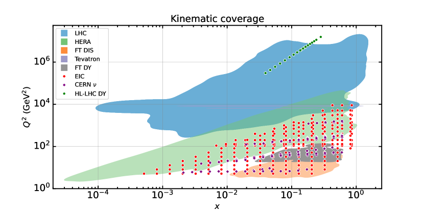
In Fig. 1 we display the kinematic coverage of the data (shaded region) and projected data (scattered points) used in this study. The full list is provided in the Appendix. The green shaded area corresponds to the HERA measurements Aaron et al. (2010); Abramowicz et al. (2013, 2015), the orange area to the Fixed-Target DIS data Arneodo et al. (1997); Whitlow et al. (1992); Benvenuti et al. (1989); Onengut et al. (2006); Goncharov et al. (2001), the purple lines to the Tevatron measurements Abazov et al. (2008a); Aaltonen et al. (2011); Abazov et al. (2008b, c, 2013, 2015), the blue area corresponds to LHC data Aad et al. (2012a); Aaboud et al. (2017a); Aad et al. (2014, 2013a); Chatrchyan et al. (2012, 2014); Chatrchyan et al. (2013a); Khachatryan et al. (2016a); Aaij et al. (2013, 2015a, 2015b, 2016a); Aad et al. (2016a); Aaboud et al. (2017b); Aaij et al. (2016b); Aad et al. (2016b); Aaij et al. (2016c); Aad et al. (2016c); Khachatryan et al. (2015a); Aaboud et al. (2018); Sirunyan et al. (2017); Aad et al. (2012b, 2013b, 2015); Chatrchyan et al. (2013b); Khachatryan et al. (2016b); Aaboud et al. (2017c); Khachatryan et al. (2017); Aad et al. (2016d); Aaboud et al. (2017d) and the grey one to Fixed-Target Drell-Yan (FTDY) measurements Adams et al. (1996); Towell et al. (2001a, b) included in the fit. The scattered points correspond to projected data for the EIC and the CERN neutrino experiments as well as for high-energy DY distributions at the HL-LHC. The main benefit of additional precise measurements covering the relatively low-energy region GeV on top of the high-energy region of TeV from the HL-LHC is that such observables, contrarily to the ones measured at the HL-LHC, are not susceptible to the effects of the BSM models identified in Hammou et al. (2023), and could therefore show a tension with the high-energy data, thus flagging a BSM-induced inconsistency in the global PDF fit.
In this work, as in Ref. Hammou et al. (2023), results are based on closure-test fits, which allow a systematic study of BSM-induced effects in PDF fits by isolating them from all other effects such as missing higher order uncertainties in theory predictions and experimental inconsistencies. Closure-test fits are done by generating the central values of the data included in the fit according to a known underlying law, given by a model and a perturbative order that determine the true partonic cross sections and a reference set of PDFs representing the true structure of the proton, and let them fluctuate according to experimental uncertainties. If a PDF fitting methodology is successful and the model used in the fit is the same as the model used in the data generation, then the fitted PDFs should reproduce the underlying law and the per datapoint should be centred around one for all experiments. If however the data are generated according to a given BSM model but PDFs are fitted assuming the SM, then a closure test is successful only if the PDFs manage to absorb the BSM shifts, as schematically indicated in Eq. (1). More details about closure tests and related statistical estimators to estimate inconsistencies are given in the Appendix.
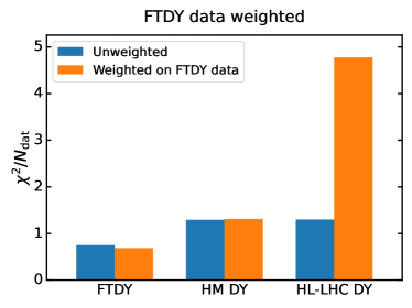
In Fig. 2 we compare the data-theory agreement for three subsets of the data included in
two closure-test fits.
In both fits, the data is generated by injecting the model discussed in Farina et al. (2017); Greljo et al. (2021); Hammou et al. (2023)
with TeV and , and PDFs are fitted assuming the SM. Details of the model under consideration are summarised
in the Appendix.
The three experimental subsets correspond to fixed-target Drell-Yan (FTDY) data, the full LHC Run I and Run II high-mass DY
data (HM DY) included in the NNPDF4.0 global fit Aad et al. (2013a); Chatrchyan
et al. (2013a); Aad et al. (2016e); Khachatryan et al. (2015b); Sirunyan et al. (2019),
and HL-LHC high-mass DY projections (HL-LHC) that were considered in Abdul Khalek et al. (2018); Greljo et al. (2021); Iranipour and Ubiali (2022); Hammou et al. (2023); Costantini et al. (2024)
to assess the potential impact of high-mass HL-LHC DY distributions on the PDFs.
The height of the histogram bars represents the per datapoint for
each data category as obtained in two fits: a closure test performed on the global NNPDF4.0 dataset augmented by
the HL-LHC projections (blue bars) and the same closure test in which more weight is given to the FTDY data (orange bars).
Details about how weighted fits are performed are given in the Appendix. The BSM model that we inject in the data affects
mostly the HL-LHC DY projections and, although moderately, the Run I and Run II high-mass DY
distributions.
As we can see, the closure-test fit associated to the blue bars is successful, indicating that the
PDF parametrisation absorbs the effects of the BSM model injected in the data. In particular
the fit quality of the HL-LHC data is extremely good, thus the BSM-induced inconsistency would not be
spotted in the consistency checks across datasets that PDF fitters routinely run.
The orange bars instead correspond to a fit in which the FTDY data was given more weight, thus features smaller uncertainties and
has a stronger pull on the fit. In that case the per data point for the FTDY data
improves, while the one of the HL-LHC projections deteriorates to a level that an inconsistency would
be spotted and these distributions would not be included in a global PDF analysis.
Typically in a PDF fit an experiment consisting of datapoints is considered inconsistent with the bulk of the other
data included in the fit if the per datapoint exceeds a critical threshold of , and
if its deviation from 1 in terms of the standard deviation of a distribution exceeds the critical threshold of 2,
namely .
To summarise, in the standard fit (blue bars) the FTDY data is not precise enough to flag the BSM-induced bias in the PDFs.
However, when extra weight is given to it, the of the HL-LHC increases dramatically, flagging the BSM-induced bias (orange bars).
The reason behind this finding is that the low-energy FTDY data, thanks to a combination of proton and isoscalar targets
constrain the ratio at large , thus increasing the tension with the HL-LHC pull on the anti-quarks.
While FTDY experiments are not currently planned by the HEP community, the EIC Aschenauer et al. (2019); Accardi et al. (2016) has been approved by the United States Department of Energy at Brookhaven National Laboratory, and could record the first scattering events as early as 2030.
Our analysis starts by considering the constraining power of the EIC projections that were considered in Khalek et al. (2021). The datapoints added to the PDF fits are listed in Table 4 in the Appendix, and their kinematic coverage is displayed in Fig. 1. We consider measurements of charged-current (CC) and neutral-current (NC) DIS processes, using both electrons and positrons as projectiles and both protons and neutrons as targets. Although the EIC will be able to use a greater variety of heavy ions as targets, we focus on the ones susceptible to constrain the proton PDF. We added these observables to the PDF fit dataset alongside the projected data from the HL-LHC that is susceptible to signs of the BSM model considered in this work and performed several fits for different masses by keeping its flavour-universal coupling .
The main observation is that the inclusion of EIC projections alongside the HL-LHC ones makes a significant difference in the ability of the large- antiquark distributions to shift and fit away the BSM signal injected in the tails of the DY distributions. This can be observed in Fig. 3. There we display the and distributions across 1000 random instances of the data generation in the closure-test fits for the datasets that are mostly affected by BSM corrections, in this case the HL-LHC CC DY projections. Looking at the blue and orange histograms, we observe that the global closure-test fit (in which data are generated according to a model with TeV and PDFs are fitted assuming the SM) displays the same good fit quality as the baseline (in which data are generated according to the SM and PDFs are fitted assuming the SM). As it was pointed out in Ref. Hammou et al. (2023) the value of TeV corresponds to the maximal BSM threshold, i. e. to the lowest that can be absorbed by the PDFs without deteriorating the of the fit, particularly of the BSM-affected data. The situation changes if the EIC projections as included. Indeed the red dotted histogram shows that the inclusion of this data would prevent PDFs from absorbing new physics, as the peak of the and distributions shifts beyond the critical values of 1.5 and 2.0 respectively that would flag up the HL-LHC CC DY projections as inconsistent with the bulk of the datasets included in the analysis, hence it would exclude it from the global PDF fit.
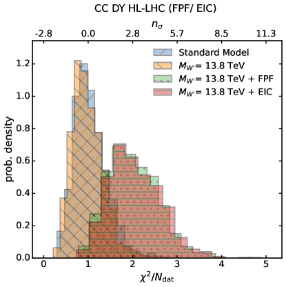
Next we assess the effect of the CERN neutrino data. The recent observation of LHC neutrinos by the FASER Abreu et al. (2024, 2023); Mammen Abraham et al. (2024) and SND Acampora et al. (2024); Albanese et al. (2023) far-forward experiments demonstrates that neutrino beams produced by collisions at the LHC can be deployed for physics studies Cruz-Martinez et al. (2024). Beyond the ongoing Run III, a dedicated suite of upgraded far-forward neutrino experiments would be hosted by the proposed Forward Physics Facility (FPF) Anchordoqui et al. (2022); Feng et al. (2023) operating concurrently with the HL-LHC. We now investigate whether the projected measurements at the two facilities considered in Cruz-Martinez et al. (2024) might provide a similar handle on the proton structure as the EIC structure function measurements, which would prevent BSM-induced bias in PDF fits. Here we only consider CC DIS processes, where the projectiles are neutrinos and anti-neutrinos, coming from the LHC beam, hitting isoscalar targets and the processes associated with charm production. As in Cruz-Martinez et al. (2024) we ignore the SND Run III projections as the current statistics is too little ro produce faithful projected data. The details of the datasets are presented in Tab. 5 in the Appendix and the kinematic coverage is displayed in Fig. 1. Looking at the green histogram in Fig. 3, we observe that, analogously to what happens in the case of the EIC, the inclusion of the FPF projections would shift the distribution for the HL-LHC high mass DY data and would flag them up as inconsistent with the bulk of other data included in the fit. Note that the main constraint comes from the proposed upgraded far-forward neutrino experiments as FASER has little impact on the PDFs.
The main finding is summarised in Fig. 4, in which we compare the data, featuring the BSM signal, i. e. the depletion in the tails associated with a new heavy with TeV and , to the SM theoretical predictions obtained with a BSM-biased set of PDFs (green line) or with a set of PDFs obtained from a joint fit of the HL-LHC data and the FPF+EIC data, in which the CC HL-LHC data get flagged and excluded from the fit (red line), or finally with the true SM PDFs (black line).
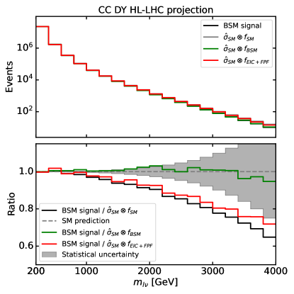
The inset shows the ratio between the BSM signal and the SM predictions for each of the PDF sets.
The green line closely matching the SM prediction demonstrates that the BSM-biased PDFs mimic the BSM signals present in the data and erase the deviation from the SM that should be observed, as in Eq. (1). As a result, using these PDFs in theoretical predictions would hide the BSM signal. This wouldn’t occur if the true PDFs (represented by the black line, which we wouldn’t know in reality) were used. However, the red line—derived from fitting the global dataset, including only the NC HL-LHC data compatible with EIC+FPF data—closely matches the black line and would allow us to detect the BSM signal.
To summarise, in this work we have identified low-energy datasets that constrain the large- region and can be included in PDF fits, enabling the safe integration of high-energy constraints from the HL-LHC. Our results show that potential BSM effects, which might otherwise be absorbed into the PDFs, can be fully disentangled in high-energy measurements. Incorporating EIC and FPF measurements in a global PDF analysis will help minimise the risk of BSM-induced bias in PDF fits and allow for more consistent identification of BSM effects in high-energy data, which can then be analysed separately.
A natural follow-up of our current study would be the extension to more complex BSM scenarios affecting both the large- quarks and gluons. Both the code and the projected data used in this study are publicly available at the SIMUnet Costantini et al. (2024) repository111https://github.com/HEP-PBSP/SIMUnet. Users are encouraged to test the robustness of our findings against different new physics scenarios and experimental projections.
Acknowledgements.
We are grateful to Juan Rojo for his precious suggestions concerning the presentation of our results. We thank Juan Rojo, Tanjona Rabemananjara and Juan Cruz-Martinez for providing us with the FPF projections and the corresponding theoretical predictions. We thank Emanuele Nocera for his assistance in identifying the EIC projected data and in generating theoretical predictions. We are most grateful for Felix Hekhorn for his precious help in using EKO and YADISM to generate interpolating grids for DIS observables. E. H. and M.U. are supported by the European Research Council under the European Union’s Horizon 2020 research and innovation Programme (grant agreement n.950246), and partially by the STFC consolidated grant ST/T000694/1 and ST/X000664/1.
References
- Baglio et al. (2022) J. Baglio, C. Duhr, B. Mistlberger, and R. Szafron, JHEP 12, 066 (2022), eprint 2209.06138.
- Amoroso et al. (2022) S. Amoroso et al., Acta Phys. Polon. B 53, 12 (2022), eprint 2203.13923.
- Ubiali (2024) M. Ubiali (2024), eprint 2404.08508.
- Ball et al. (2022a) R. D. Ball et al. (NNPDF), Eur. Phys. J. C 82, 428 (2022a), eprint 2109.02653.
- Hammou et al. (2023) E. Hammou, Z. Kassabov, M. Madigan, M. L. Mangano, L. Mantani, J. Moore, M. M. Alvarado, and M. Ubiali, JHEP 11, 090 (2023), eprint 2307.10370.
- Costantini et al. (2024) M. N. Costantini, E. Hammou, Z. Kassabov, M. Madigan, L. Mantani, M. Morales Alvarado, J. M. Moore, and M. Ubiali (PBSP), Eur. Phys. J. C 84, 805 (2024), eprint 2402.03308.
- Farina et al. (2017) M. Farina, G. Panico, D. Pappadopulo, J. T. Ruderman, R. Torre, and A. Wulzer, Phys. Lett. B772, 210 (2017), eprint 1609.08157.
- Greljo et al. (2021) A. Greljo, S. Iranipour, Z. Kassabov, M. Madigan, J. Moore, J. Rojo, M. Ubiali, and C. Voisey, JHEP 07, 122 (2021), eprint 2104.02723.
- Abdul Khalek et al. (2022a) R. Abdul Khalek et al., Nucl. Phys. A 1026, 122447 (2022a), eprint 2103.05419.
- Abdul Khalek et al. (2022b) R. Abdul Khalek et al. (2022b), eprint 2203.13199.
- Abreu et al. (2024) H. Abreu et al. (FASER), JINST 19, P05066 (2024), eprint 2207.11427.
- Abreu et al. (2023) H. Abreu et al. (FASER), Phys. Rev. Lett. 131, 031801 (2023), eprint 2303.14185.
- Mammen Abraham et al. (2024) R. Mammen Abraham et al. (FASER), Phys. Rev. Lett. 133, 021802 (2024), eprint 2403.12520.
- Acampora et al. (2024) G. Acampora et al. (SND@LHC), JINST 19, P05067 (2024), eprint 2210.02784.
- Albanese et al. (2023) R. Albanese et al. (SND@LHC), Phys. Rev. Lett. 131, 031802 (2023), eprint 2305.09383.
- Anchordoqui et al. (2022) L. A. Anchordoqui et al., Phys. Rept. 968, 1 (2022), eprint 2109.10905.
- Feng et al. (2023) J. L. Feng et al., J. Phys. G 50, 030501 (2023), eprint 2203.05090.
- Accardi et al. (2016) A. Accardi et al., Eur. Phys. J. A 52, 268 (2016), eprint 1212.1701.
- Aschenauer et al. (2019) E. C. Aschenauer, S. Fazio, J. H. Lee, H. Mantysaari, B. S. Page, B. Schenke, T. Ullrich, R. Venugopalan, and P. Zurita, Rept. Prog. Phys. 82, 024301 (2019), eprint 1708.01527.
- Khalek et al. (2021) R. A. Khalek, J. J. Ethier, E. R. Nocera, and J. Rojo, Phys. Rev. D 103, 096005 (2021), eprint 2102.00018.
- Cruz-Martinez et al. (2024) J. M. Cruz-Martinez, M. Fieg, T. Giani, P. Krack, T. Mäkelä, T. R. Rabemananjara, and J. Rojo, Eur. Phys. J. C 84, 369 (2024), eprint 2309.09581.
- Boughezal et al. (2020) R. Boughezal, F. Petriello, and D. Wiegand, Phys. Rev. D 101, 116002 (2020), eprint 2004.00748.
- Bissolotti et al. (2023) C. Bissolotti, R. Boughezal, and K. Simsek (2023), eprint 2307.09459.
- Aleksa et al. (2022) M. Aleksa et al., 2/2022 (2022).
- Ball et al. (2022b) R. D. Ball, A. Candido, S. Forte, F. Hekhorn, E. R. Nocera, J. Rojo, and C. Schwan, Eur. Phys. J. C 82, 1160 (2022b), eprint 2209.08115.
- Anataichuk et al. (2023) A. Anataichuk et al. (2023), eprint 2310.19638.
- Fiaschi et al. (2022) J. Fiaschi, F. Giuli, F. Hautmann, and S. Moretti, JHEP 02, 179 (2022), eprint 2111.09698.
- Aaron et al. (2010) F. Aaron et al. (H1 and ZEUS), JHEP 1001, 109 (2010), eprint 0911.0884.
- Abramowicz et al. (2013) H. Abramowicz et al. (H1 , ZEUS), Eur.Phys.J. C73, 2311 (2013), eprint 1211.1182.
- Abramowicz et al. (2015) H. Abramowicz et al. (ZEUS, H1), Eur. Phys. J. C75, 580 (2015), eprint 1506.06042.
- Arneodo et al. (1997) M. Arneodo et al. (New Muon), Nucl. Phys. B483, 3 (1997), eprint hep-ph/9610231.
- Whitlow et al. (1992) L. W. Whitlow, E. M. Riordan, S. Dasu, S. Rock, and A. Bodek, Phys. Lett. B282, 475 (1992).
- Benvenuti et al. (1989) A. C. Benvenuti et al. (BCDMS), Phys. Lett. B223, 485 (1989).
- Onengut et al. (2006) G. Onengut et al. (CHORUS), Phys. Lett. B632, 65 (2006).
- Goncharov et al. (2001) M. Goncharov et al. (NuTeV), Phys. Rev. D64, 112006 (2001), eprint hep-ex/0102049.
- Abazov et al. (2008a) V. M. Abazov et al. (D0), Phys. Rev. Lett. 101, 211801 (2008a), eprint 0807.3367.
- Aaltonen et al. (2011) T. Aaltonen et al. (CDF and D0) (2011), eprint 1103.3233.
- Abazov et al. (2008b) V. M. Abazov et al. (D0), Phys. Rev. Lett. 101, 062001 (2008b), eprint 0802.2400.
- Abazov et al. (2008c) V. M. Abazov et al. (D0), Phys. Lett. B666, 23 (2008c), eprint 0803.2259.
- Abazov et al. (2013) V. M. Abazov et al. (D0), Phys.Rev. D88, 091102 (2013), eprint 1309.2591.
- Abazov et al. (2015) V. M. Abazov et al. (D0), Phys. Rev. D91, 032007 (2015), [Erratum: Phys. Rev.D91,no.7,079901(2015)], eprint 1412.2862.
- Aad et al. (2012a) G. Aad et al. (ATLAS), Phys.Rev. D85, 072004 (2012a), eprint 1109.5141.
- Aaboud et al. (2017a) M. Aaboud et al. (ATLAS), Eur. Phys. J. C77, 367 (2017a), eprint 1612.03016.
- Aad et al. (2014) G. Aad et al. (ATLAS), JHEP 06, 112 (2014), eprint 1404.1212.
- Aad et al. (2013a) G. Aad et al. (ATLAS), Phys.Lett. B725, 223 (2013a), eprint 1305.4192.
- Chatrchyan et al. (2012) S. Chatrchyan et al. (CMS), Phys.Rev.Lett. 109, 111806 (2012), eprint 1206.2598.
- Chatrchyan et al. (2014) S. Chatrchyan et al. (CMS), Phys.Rev. D90, 032004 (2014), eprint 1312.6283.
- Chatrchyan et al. (2013a) S. Chatrchyan et al. (CMS), JHEP 1312, 030 (2013a), eprint 1310.7291.
- Khachatryan et al. (2016a) V. Khachatryan et al. (CMS), Eur. Phys. J. C76, 469 (2016a), eprint 1603.01803.
- Aaij et al. (2013) R. Aaij et al. (LHCb), JHEP 1302, 106 (2013), eprint 1212.4620.
- Aaij et al. (2015a) R. Aaij et al. (LHCb), JHEP 08, 039 (2015a), eprint 1505.07024.
- Aaij et al. (2015b) R. Aaij et al. (LHCb), JHEP 05, 109 (2015b), eprint 1503.00963.
- Aaij et al. (2016a) R. Aaij et al. (LHCb), JHEP 01, 155 (2016a), eprint 1511.08039.
- Aad et al. (2016a) G. Aad et al. (ATLAS), JHEP 08, 009 (2016a), eprint 1606.01736.
- Aaboud et al. (2017b) M. Aaboud et al. (ATLAS), JHEP 12, 059 (2017b), eprint 1710.05167.
- Aaij et al. (2016b) R. Aaij et al. (LHCb), JHEP 10, 030 (2016b), eprint 1608.01484.
- Aad et al. (2016b) G. Aad et al. (ATLAS), Phys. Lett. B 759, 601 (2016b), eprint 1603.09222.
- Aaij et al. (2016c) R. Aaij et al. (LHCb), JHEP 09, 136 (2016c), eprint 1607.06495.
- Aad et al. (2016c) G. Aad et al. (ATLAS), Eur. Phys. J. C76, 291 (2016c), eprint 1512.02192.
- Khachatryan et al. (2015a) V. Khachatryan et al. (CMS), Phys. Lett. B749, 187 (2015a), eprint 1504.03511.
- Aaboud et al. (2018) M. Aaboud et al. (ATLAS), JHEP 05, 077 (2018), [Erratum: JHEP 10, 048 (2020)], eprint 1711.03296.
- Sirunyan et al. (2017) A. M. Sirunyan et al. (CMS), Phys. Rev. D 96, 072005 (2017), eprint 1707.05979.
- Aad et al. (2012b) G. Aad et al. (ATLAS), Phys. Rev. D86, 014022 (2012b), eprint 1112.6297.
- Aad et al. (2013b) G. Aad et al. (ATLAS), Eur.Phys.J. C73, 2509 (2013b), eprint 1304.4739.
- Aad et al. (2015) G. Aad et al. (ATLAS), JHEP 02, 153 (2015), [Erratum: JHEP09,141(2015)], eprint 1410.8857.
- Chatrchyan et al. (2013b) S. Chatrchyan et al. (CMS), Phys.Rev. D87, 112002 (2013b), eprint 1212.6660.
- Khachatryan et al. (2016b) V. Khachatryan et al. (CMS), Eur. Phys. J. C76, 265 (2016b), eprint 1512.06212.
- Aaboud et al. (2017c) M. Aaboud et al. (ATLAS), JHEP 09, 020 (2017c), eprint 1706.03192.
- Khachatryan et al. (2017) V. Khachatryan et al. (CMS), JHEP 03, 156 (2017), eprint 1609.05331.
- Aad et al. (2016d) G. Aad et al. (ATLAS), JHEP 08, 005 (2016d), eprint 1605.03495.
- Aaboud et al. (2017d) M. Aaboud et al. (ATLAS), Phys. Lett. B 770, 473 (2017d), eprint 1701.06882.
- Adams et al. (1996) M. R. Adams et al. (E665), Phys. Rev. D54, 3006 (1996).
- Towell et al. (2001a) R. S. Towell et al. (FNAL E866/NuSea), Phys. Rev. D64, 052002 (2001a), eprint hep-ex/0103030.
- Towell et al. (2001b) R. S. Towell et al. (NuSea), Phys. Rev. D 64, 052002 (2001b), eprint hep-ex/0103030.
- Aad et al. (2016e) G. Aad et al. (ATLAS), JHEP 08, 009 (2016e), eprint 1606.01736.
- Khachatryan et al. (2015b) V. Khachatryan et al. (CMS), Eur. Phys. J. C75, 147 (2015b), eprint 1412.1115.
- Sirunyan et al. (2019) A. M. Sirunyan et al. (CMS), JHEP 12, 059 (2019), eprint 1812.10529.
- Abdul Khalek et al. (2018) R. Abdul Khalek, S. Bailey, J. Gao, L. Harland-Lang, and J. Rojo, Eur. Phys. J. C78, 962 (2018), eprint 1810.03639.
- Iranipour and Ubiali (2022) S. Iranipour and M. Ubiali, JHEP 05, 032 (2022), eprint 2201.07240.
- Ball et al. (2015) R. D. Ball et al. (NNPDF), JHEP 04, 040 (2015), eprint 1410.8849.
- Del Debbio et al. (2022) L. Del Debbio, T. Giani, and M. Wilson, Eur. Phys. J. C 82, 330 (2022), eprint 2111.05787.
- Alwall et al. (2014) J. Alwall, R. Frederix, S. Frixione, V. Hirschi, F. Maltoni, O. Mattelaer, H. S. Shao, T. Stelzer, P. Torrielli, and M. Zaro, JHEP 07, 079 (2014), eprint 1405.0301.
Appendix A Estimators and list of data and pseudo-data
In this Appendix, we provide additional information about the methodology and the definition of the statistical estimators used in our analysis. We also provide a list of experimental data and pseudo-data that we include, as well as details on the BSM model that we consider throughout the paper. Additionally we show how our findings vary as a weaker BSM signal is injected in the data. We investigate what is the maximal BSM signal that may be absorbed in PDF fit even in the presence of EIC and FPF data and what the effect would be on indirect BSM searches.
Closure test.
In order to systematically study possible BSM-induced bias in PDF fits, we work in a setting in which we assume we know the underlying law of nature. In our case the law of nature consists of the true PDFs, which are low-energy quantities that have nothing to do with new physics, and the true UV complete Lagrangian, which at low energy is well approximated by the SM Lagrangian but which comprises heavy new particles. We use these assumptions to generate the pseudo-data in our analysis. We inject the effect of the new particles that we introduce in the Lagrangian in the articifially generated data, and their effect will be visible in some high-energy distributions depending on the underlying model. The methodology we use throughout this study is based on the NNPDF closure-test framework, first introduced in Ref. Ball et al. (2015), and explained in more detail in Ref. Del Debbio et al. (2022). Various statistical estimators are applied to check the quality of the fit (in broad terms, assessing its difference from the true PDFs), hence verifying the accuracy of the fitting methodology.
Detection of inconsistencies in global PDF fits.
Once we produce a closure test fit, in which PDFs have been fitted assuming the SM but the artificial data have been produced according to a given BSM model we check whether it is possible to detect BSM-induced bias in the PDF fit, i.e. whether the datasets which are affected by he given BSM appear inconsistent with the bulk of the data in the global analysis and are poorly described by the resulting PDFs. To quantitatively address this point, we use the NNPDF dataset selection criteria, discussed in detail in Ball et al. (2022a). We consider both the -statistic of the resulting fit to each dataset entering the fit, and also consider the number of standard deviations
| (2) |
of the -statistics from the expected for each dataset. If and for a particular dataset, the dataset would be flagged by the NNPDF selection criteria, indicating an inconsistency with the other data entering the fit.
Weighted fits.
There are two possible outcomes from performing such a dataset selection analysis on a fit. In the first instance, the datasets affected by NP are flagged by the dataset selection criterion. If a dataset is flagged according to this condition, then a weighted fit is performed, i.e. a fit in which a dataset is given a larger weight inversely proportional to the number of datapoints, namely
| (3) |
with
| (4) |
If the data-theory agreement improves by setting it below thresholds and the data-theory agreement of the other datasets does not deteriorate in any statistically relevant way, then the dataset is kept, else the dataset is discarded, on the basis of the inconsistency with the remaining datasets.
Statistical distributions.
Moreover, to check if the flag raised in the post-fit analysis is statistically significant, we repeat the and computations across 1000 random instances of the data generation in the closure-test fits (corresponding to independent runs of the Universe). We check it both globally and for each individual datasets, with a special emphasis on the datasets that are mostly affected by the BSM corrections associated to the given model. If the and distributions are peaked above the critical thresholds of 1.5 and 2 respectively, then the weighted fit procedure is activated and the inconsistency is assessed according to the methodology outlined above.
BSM model.
The model that we consider thoughout this paper consists of the triplet field , where denotes an index, with mass and coupling coefficient by . The model is explained in details in Refs. Farina et al. (2017); Greljo et al. (2021) and is described by the Lagrangian:
| (5) |
where the sum runs over the left-handed fermions: . The generators are given by where are the Pauli matrices. The kinetic term is given by . The covariant derivative is given by . The mixing with the SM gauge fields is neglected. The leading effect of this model on the dataset included in our analysis is to modify the Drell-Yan and deep inelastic scattering observables, both charged current and neutral current. The tree-level matching of to the dimension-6 operators in the SMEFT is described in details in Ref. Greljo et al. (2021). There it is shown that the impact at the LHC energy is dominated by the four-fermion interactions, which sum to:
| (6) |
which is typically described by the parameter:
| (7) |
Using Fermi’s constant, one can write the relation between the UV parameters and as
| (8) |
By fixing , each can be associated to a value of .
Datasets included.
We use all datasets included in the NNPDF4.0 global analysis Ball et al. (2022a). The high-mass Drell-Yan measurements from ATLAS and CMS are impacted by the model we consider, we provide details on the datapoints in Tab. 1. Several fixed-target Drell-Yan measurements from Fermilab with proton (p) and deuteron (d) targets probe the same processes at much lower energies. The effects of new physics are much more suppressed and they remain compatible with the SM predictions. More details is provided in Tab. 2. On top of the existing measurements, we include the high-mass Drell-Yan projections that were introduced in Greljo et al. (2021), inspired by the HL-LHC projections studied in Abdul Khalek et al. (2018). The invariant mass distribution projections are generated at 14 TeV assuming an integrated luminosity of 6 ab-1 (3 ab-1 collected by ATLAS and 3 ab-1 by CMS). Both in the case of NC and CC Drell-Yan cross sections, the MC data were generated using the MadGraph5 aMCatNLO NLO Monte Carlo event generator Alwall et al. (2014) with additional -factors to include the NNLO QCD and NLO EW corrections. The MC data consist of four datasets (associated with NC/CC distributions with muons/electrons in the final state), each comprising 16 bins in the invariant mass distribution or transverse mass distributions with both and greater than 500 GeV , with the highest energy bins reaching = 4 TeV ( = 3.5 TeV) for NC (CC) data. The rationale behind the choice of number of bins and the width of each bin was outlined in Ref. Greljo et al. (2021), and stemmed from the requirement that the expected number of events per bin was big enough to ensure the applicability of Gaussian statistics. The choice of binning for the distribution at the HL-LHC is displayed in Fig. 5.1 of Ref. Greljo et al. (2021). The details of the datasets included in the fit are presented in Tab. 3.
| Observable [TeV] ATLAS 13 7 48 8 CMS 132 7 132 7 43 13 Table 1: Summary of the high-mass Drell-Yan data included in NNPDF4.0 Ball et al. (2022a). | Observable [GeV] NuSea (E866) (d) 15 800 (p) 184 800 E605 119 38.8 SeaQuest (E905) (d) 6 120 Table 2: Summary of the fixed-target Drell-Yan data included in NNPDF4.0 Ball et al. (2022a). | Observable [TeV] Charged Current 16 14 16 14 Neutral Current 12 14 12 14 Table 3: Summary of the HL-LHC projected data included in this work, taken from Ref. Greljo et al. (2021). |
As far as the EIC projections are concerned, we consider those that were built in Ref. Khalek et al. (2021), in particular the measurements of charged-current (CC) and neutral-current (NC) DIS processes, using both electrons and positrons as projectiles and both protons and neutrons as targets. Details about the projections used are presented in Tab. 4. We tested both the optimistic and pessimistic scenarios which vary in terms of how many datapoints can be collected. We found that the choice of scenario does not impact much our results.
For the FPF data, we consider the projected data built in Ref. Cruz-Martinez et al. (2024). The focus is on charged-current DIS processes, where the projectiles are neutrinos and anti-neutrinos, coming from the LHC beam, hitting isoscalar targets and the processes associated with charm production. For each of the far-forward LHC neutrino experiments the pseudo-rapidity coverage, target material, the acceptance for the charged lepton and hadronic final state, and the expected reconstruction performance are identified in Cruz-Martinez et al. (2024) assuming that FASER and SND acquire data for Run III with = 150 fb-1. SND projections are too statistically insignificant to be included in the fit, due to the little statistics collected so far. As far as the FPF facility is concerned, FASER2, AdvSND, and FLArE take data for the complete HL-LHC period, with = 3 ab-1. The complete set of projected data that is included is summarised in Tab. 5.
| Observable [GeV] [fb] Charged Current 89 (89) 140.7 100 89 (89) 140.7 10 Neutral Current (proton) 181 (131) 140.7 100 181 (131) 63.2 100 126 (91) 44.7 100 87 (76) 28.6 100 181 (131) 140.7 10 181 (131) 63.2 10 126 (91) 44.7 10 87 (76) 28.6 10 Neutral Current (deuteron) 116 (116) 89.0 10 107 (107) 66.3 10 76 (76) 28.6 10 116 (116) 89.0 10 107 (107) 66.3 10 76 (76) 28.6 10 Table 4: Summary of the EIC projected data included in this work, taken from Ref. Khalek et al. (2021). | Observable FASER 22 16 FLArE 43 39 31 19 FASER2 44 39 38 30 AdvSND 33 29 17 Table 5: Summary of the FPF projected data included in this work, taken from Ref. Cruz-Martinez et al. (2024). |
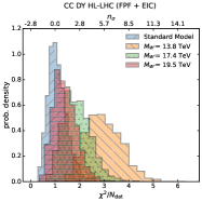
Maximal BSM threshold.
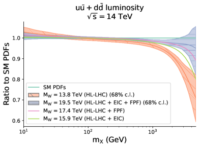
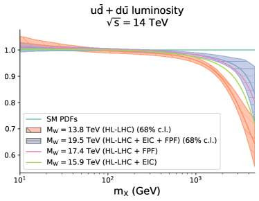
To conclude, we consider how the maximal BSM threshold, i. e. the maximal BSM signal that can be absorbed by PDFs in a global fit, shifts as we include FPF and EIC projected data. Clearly, if we inject in the data the effect of a new heavy flavour-universal , with mass larger than TeV, the depletion in the high-energy tails measured at the HL-LHC will be less significant and thus the effect can still be fitted away in the PDFs. In this appendix we investigate by how much the EIC and CERN neutrino data would shift the maximal BSM threshold and whether the impact of the BSM bias - pushed at a higher threshold - would visibly impact the PDFs and thus possibly hamper the interpretation of indirect new physics searches. To answer this question, we made a scan over , by injecting increasingly large values of the mass, until the signal can be absorbed even in the presence of precise EIC and CERN neutrino data in a PDF global analysis. The summary results of the analysis are displayed in Fig. 5. There we see that, as we increase the value of in our BSM model, thus decrease the size of the BSM corrections injected in the data, we have to get to TeV (orange histogram) for the signal to be absorbed in the PDFs.
Finally, we ask ourselves what is the effect of the new physics absorption now that the threshold has been pushed to a significantly larger value. Is this still going to spoil the interpretation of indirect BSM searches? To answer this question we assess the impact of the injection of our new physics model in the data on the fitted PDFs, by looking at the integrated luminosities for the parton pair , which is defined as:
| (9) |
where is the PDF corresponding to the parton flavour , and the integration limits are defined by:
| (10) |
In particular, we focus on the luminosities that are most constrained by the NC and CC Drell-Yan data respectively, namely
| (11) | ||||
| (12) |
In Fig. 6 we show how the addition of the new projected data mitigates the BSM-induced PDF bias. We compare the NC and CC PDF luminosities defined in Eqs. (11) and (12) respectively as a function of , which in the case of NC can be identified with the invariant mass of the produced leptons and in the case of CC can be identified with the transverse mass of the lepton-neutrino pair. We compare the luminosities obtained in a closure test in which the data have been generated by injecting a model with set at different values and the data fitted assuming the SM. Each of the curves is compared to the true SM luminosities. The orange band represents the luminosities fitted on the whole NNPDF4.0 dataset plus the HL-LHC projected data displayed in Table 3 with a TeV signal injected in the data and the fit performed assuming the SM. Here the result is the same as the one presented in Ref. Hammou et al. (2023), namely the luminosities shift significantly as the PDFs have completely absorbed the BSM signal. On the other hand, if the EIC and the CERN forward neutrino projected data is included alongside the HL-LHC one, then the maximal BSM signal that can be absorbed corresponds to TeV. The corresponding PDF luminosities are displayed in blue. We observe a systematic reduction of the discrepancy with the true SM luminosities. In the case of the luminosity, the fit including EIC and CERN forward neutrino projections almost completely suppresses the discrepancy while for the a visible shift remains but its effect is greatly reduced. The intermediate case in which only EIC projections or only FPF projections are included are shown with only their central values in green and pink respectively, according to the maximal BSM signal that can be absorbed in each of these cases. To conclude, if the EIC and FPF projections are included in a global PDF analysis alongside the HL-LHC high-mass Drell-Yan distributions, the maximal BSM threshold, i. e. the maximal BSM signal that can be absorbed by PDFs in a global fit, shifts to larger values. As a result, while the effect can still be fitted away in the PDFs, the consequences are much milder and the BSM-biased PDFs are statistically undistinguishable from the true SM PDFs, thus effectively disentangling PDF effects from BSM effects.