Multi-orbital two-particle self-consistent approach – strengths and limitations

Jonas B. Profe^1$\star$, Jiawei Yan², Karim Zantout¹, Philipp Werner² and Roser Valentí¹

Abstract

Extending many-body numerical techniques which are powerful in the context of simple model calculations to the realm of realistic material simulations can be a challenging task. Realistic systems often involve multiple active orbitals, which increases the complexity and numerical cost because of the large local Hilbert space and the large number of interaction terms or sign-changing off-diagonal Green’s functions. The two-particle self-consistent approach (TPSC) is one such many-body numerical technique, for which multi-orbital extensions have proven to be involved due to the substantially more complex structure of the local interaction tensor. In this paper we extend earlier multi-orbital generalizations of TPSC by setting up two different variants of a fully self-consistent theory for TPSC in multi-orbital systems. We first investigate the strengths and limitations of the approach analytically, and then benchmark both variants against exact diagonalization (ED) and dynamical mean field theory (DMFT) results. We find that the exact behavior of the system can be faithfully reproduced in the weak coupling regime, while at stronger couplings the performance of the two approaches strongly depends on details of the system.

Copyright attribution to authors.
This work is a submission to SciPost Physics Lecture Notes.
License information to appear upon publication.
Publication information to appear upon publication. Received Date
Accepted Date
Published Date

1 Introduction

Solving the many-body problem of interacting electrons remains a central challenge in condensed matter physics. Analytical solutions can only be found in rare cases [1, 2], necessitating the development of advanced numerical methods such as Density Functional Theory [3, 4], Quantum Monte Carlo (QMC) [5, 6, 7, 8, 9, 10], DMRG and other Tensor network approaches [11, 12, 13], Dynamical Mean-Field Theory and its extensions [14, 15, 16, 17, 18, 19], variational (neural) quantum states [20, 21, 22, 10, 23, 24, 25] or various diagrammatic methods [26, 27, 28, 29, 30, 31]. With the use of these approaches the community gained insights into correlated electron physics, e.g. by developing an understanding of Mott physics [32, 33, 34, 35], (unconventional) superconductivity [36, 37, 38, 39, 40], the pseudogap phase [41, 42], magnetism and spin liquids [43, 44, 45] and charge ordered states [46, 47, 48]. In recent years, a coherent picture has emerged for some single-orbital models, with a variety of numerical approaches producing consistent results for ground state energies, mass renormalizations, etc. [49, 50, 51], which shifts the frontiers of method development to more complex models and setups.

Going beyond single orbital models, it is natural to consider multi-orbital extensions which are relevant for real materials. In such multi-orbital models, the complexity of the orbital structure introduces new competing energy scales, as exemplified by the Hund’s metals [52, 53, 54, 55, 56] which turn out to be relevant for a large variety of materials including iron-based superconductors [57, 58, 59, 54, 60], ruthenates [61, 62] and molybdates [63], to mention a few. This more intricate local structure of the interaction tensor has profound consequences for a number of numerical approaches, e.g. leading to a sign problem in some QMC variants [64] and, in general, to a larger numerical cost. Thus, extending numerical techniques to multi-orbital systems poses often not only an analytical but also a computational challenge which has to be overcome. Furthermore, approximations known to work well in the single orbital case are not guaranteed to be equally adequate for multi-orbital systems.

Numerical studies can provide guiding principles and insights into the microscopic mechanisms behind emergent phenomena. However, in cases where the employed numerical approach fails qualitatively or quantitatively, as for example in the case of some iron-based superconductors where neither DFT nor DFT+DMFT predict correct Fermi surfaces [65, 66, 67], it is important to extend the techniques and improve their accuracy. A promising route for the study of correlated materials is to extend the formalism beyond DMFT, which is a dynamical but local approach, by combining it with another numerical approach which captures the effects of spatial and temporal fluctuations [14]. For this, two different strategies have been considered in recent years. One idea is to include finite distance correlations in the DMFT itself, at the cost of a more complicated impurity problem, as in the case of cellular DMFT [68, 69, 70] and the dynamical cluster approximation [71, 72]. Alternatively, one can extend the locality-approximation of DMFT from the self-energy to some vertex-functions, as done for example in TRILEX [18] and D-TRILEX [73, 74], the dynamical-vertex approximation [17, 75] and other schemes [14, 76, 77, 78]. These approaches however typically require the calculation of local vertex functions, which is a time consuming and challenging task for complicated models [79].

One very successful numerical method for systems with weak to intermediate correlations is the two particle self-consistent (TPSC) approach [80, 81, 82], which was first formulated for the single-band Hubbard model [83, 84], and subsequently extended to multi-site [85, 86], non-$SU(2)$ [87, 88], multi-orbital [89, 66, 90, 91] and non-equilibrium [92, 93] problems. Furthermore, it has been combined with DMFT to extend its range of validity [94, 95, 96]. TPSC has been applied extensively to single orbital models [97, 98, 80, 99, 100, 101, 102, 103, 104], for which it yields remarkably accurate results [50] at a comparably low numerical cost. Its combination with DMFT does not require the calculation of a vertex, but only the two-particle density matrix, which can be evaluated at much lower numerical cost. If this methodology works reliably in multi-orbital systems, TPSC and TPSC+DMFT will become prime contenders for the study of complex correlated materials.

Motivated by these prospects, we present and benchmark in this paper two different variants of a fully self-consistent multi-orbital TPSC approach by establishing sum rules taking into account the $SU(2)$ symmetry of the system. This allows us to determine all required two-particle expectation values (TPEV) from exact sum rules, overcoming approximations that had to be applied in earlier formulations [89, 90].

The paper is structured as follows: In Section 2, we derive the central equations of TPSC from scratch and analytically discuss potential shortcomings. In Section 3.1, we analyze a density-density interaction-only model analytically within TPSC, and point out potential pitfalls. In Section 3.2 we analyze the effects of a strong Hunds-coupling. Next, in Section 3.3, we benchmark the accuracy of the self-consistently determined two-particle expectation values, by comparing the TPSC results to exact diagonalization (ED) and DMFT calculations. In addition, we compare the spin and charge susceptibilities to D-TRILEX [19] and discuss the implications of these results for the applicability of our TPSC formulations to realistic multi-orbitals models.

2 Multi-orbital TPSC

In this chapter we present two variants of the multi-orbital TPSC formalism. The derivation follows closely analogous derivations for the single orbital case [80, 82]. In the following we will consider a general tight-binding Hamiltonian with local and instantaneous interactions

$$H=t_{o_{1}^{\prime},o_{3}^{\prime}}(\boldsymbol{r}_{1}^{\prime}-\boldsymbol{r}_{3}^{\prime}) c^{\dagger}_{o_{3}^{\prime},s^{\prime}}(\boldsymbol{r}^{\prime}_{3})c_{o_{1}^{\prime},s^{\prime}}(\boldsymbol{r}_{1}^{\prime})$$ (1)

$$+\frac{1}{2}U^{s_{1}^{\prime}s_{2}^{\prime}s_{3}^{\prime}s_{4}^{\prime}}_{o_{1}^{\prime}o_{2}^{\prime}o_{3}^{\prime}o_{4}^{\prime}}c^{\dagger}_{o_{3}^{\prime},s_{3}^{\prime}}(\boldsymbol{r}^{\prime})c^{\dagger}_{o_{4}^{\prime},s_{4}^{\prime}}(\boldsymbol{r}^{\prime})c_{o_{2}^{\prime},s_{2}^{\prime}}(\boldsymbol{r}^{\prime})c_{o_{1}^{\prime},s_{1}^{\prime}}(\boldsymbol{r}^{\prime}),~{}$$

where $c^{(\dagger)}_{o_{1},s_{1}}(\tau_{1},\boldsymbol{r}_{1})$ annihilates (creates) an electron at orbital $o_{1}$ with spin $s_{1}$ at the lattice position $\boldsymbol{r}_{1}$. All primed variables are summed over. As a short hand for all non explicitly stated quantum numbers of an object we will use plain numbers as indices. We will restrict ourselves to the case of an $SU(2)$ symmetric model. To reduce the complexity, we rewrite the Hubbard interaction tensor in terms of its even and odd $SU(2)$-transforming components [105]

$$U^{s_{1}s_{2}s_{3}s_{4}}_{o_{1}o_{2}o_{3}o_{4}}=U_{o_{1}o_{2}o_{3}o_{4}}\delta_{s_{1},s_{3}}\delta_{s_{2},s_{4}}-U_{o_{1}o_{2}o_{4}o_{3}}\delta_{s_{1},s_{4}}\delta_{s_{2},s_{3}}\;.$$ (2)

Lastly, we restrict ourselves to inter-orbital-bilinear type interactions [106] (still allowing for intra-orbital interactions within this bilinear form), thus the spin independent interaction tensor is simplified to

$$U_{o_{1}o_{2}o_{3}o_{4}}=D_{o_{1},o_{4}}\delta_{o_{1},o_{3}}\delta_{o_{2},o_{4}}+C_{o_{1},o_{3}}\delta_{o_{1},o_{4}}\delta_{o_{2},o_{3}}+P_{o_{1},o_{3}}\delta_{o_{1},o_{2}}\delta_{o_{3},o_{4}},$$ (3)

where each of the contributions can be identified with a specific physical process: density-density type interactions are given by $D$, spin-flip interactions by $C$ and pair-hopping processes by $P$. TPSC can also be formulated without this restriction, however restricting the interaction allows for an easier understanding of the equations and processes involved. Thus we focus on this simplified form.

The central equation on which TPSC is built upon is the equation of motion [80], linking the product of the single particle self-energy and the Green’s function to the tensor contraction of the two-particle interaction with a two-particle expectation value (TPEV), which can be re-expressed in terms of a generalized susceptibility. For a derivation of the equation of motion, see Appendix A. With the assumption of an $SU(2)$-symmetric inter-orbital bilinear-type interaction, the equation of motion simplifies to

$$\Sigma_{1,1^{\prime}}G_{1^{\prime},5} =\frac{1}{2}U_{o_{2}^{\prime}o_{3}^{\prime}o_{4}^{\prime}o_{1}}^{s_{2}^{\prime}s_{3}^{\prime}s_{4}^{\prime}s_{1}}\braket{\mathcal{T}c^{\dagger}_{4^{\prime}}(\tau_{1},r_{1})c_{3^{\prime}}(\tau_{1},r_{1})c_{2^{\prime}}(\tau_{1},r_{1})c_{5}^{\dagger}}$$ (4)

$$=\frac{1}{2}U_{o_{2}^{\prime},o_{3}^{\prime},o_{4}^{\prime},o_{1}}\braket{\mathcal{T}c_{o_{4}^{\prime},s_{4}^{\prime}}^{\dagger}(\tau_{1},r_{1})c_{o_{3}^{\prime},s_{1}}(\tau_{1},r_{1})c_{o_{2}^{\prime},s_{4}^{\prime}}(\tau_{1},r_{1})c_{5}^{\dagger}}$$ (5)

$$\quad-\frac{1}{2}U_{o_{2}^{\prime},o_{3}^{\prime},o_{1},o_{4}^{\prime}}\braket{\mathcal{T}c_{o_{4}^{\prime},s_{4}^{\prime}}^{\dagger}(\tau_{1},r_{1})c_{o_{3}^{\prime},s_{4}^{\prime}}(\tau_{1},r_{1})c_{o_{2}^{\prime},s_{1}}(\tau_{1},r_{1})c_{5}^{\dagger}}$$

$$=U_{o_{2}^{\prime},o_{3}^{\prime},o_{4}^{\prime},o_{1}}\braket{\mathcal{T}c_{o_{4}^{\prime},s_{4}^{\prime}}^{\dagger}c_{o_{3}^{\prime},s_{1}}c_{o_{2}^{\prime},s_{4}^{\prime}}c_{5}^{\dagger}}\bar{\delta}_{s_{1},s_{4}^{\prime}}\bar{\delta}_{o_{2}^{\prime},o_{3}^{\prime}}$$ (6)

$$=\Big{(}D_{o_{4}^{\prime},o_{1}}\sum_{s_{4}^{\prime}}\bar{\delta}_{s_{1},s_{4}^{\prime}}\bar{\delta}_{o_{1},o_{4}^{\prime}}\braket{\mathcal{T}c_{o_{4}^{\prime},s_{4}^{\prime}}^{\dagger}c_{o_{1},s_{1}}c_{o_{4}^{\prime},s_{4}^{\prime}}c_{5}^{\dagger}}$$ (7)

$$\quad+C_{o_{1},o_{4}^{\prime}}\sum_{s_{4}^{\prime}}\bar{\delta}_{s_{1},s_{4}^{\prime}}\bar{\delta}_{o_{1},o_{4}^{\prime}}\braket{\mathcal{T}c_{o_{4}^{\prime},s_{4}^{\prime}}^{\dagger}c_{o_{4}^{\prime},s_{1}}c_{o_{1},s_{4}^{\prime}}c_{5}^{\dagger}}$$

$$\quad+P_{o_{2}^{\prime},o_{1}}\sum_{s_{4}^{\prime}}\bar{\delta}_{s_{1},s_{4}^{\prime}}\braket{\mathcal{T}c_{o_{1},s_{4}^{\prime}}^{\dagger}c_{o_{2}^{\prime},s_{1}}c_{o_{2}^{\prime},s_{4}^{\prime}}c_{5}^{\dagger}}\Big{)}\,,$$

where we introduced $\bar{\delta}$ as a short hand for $1-\delta$. The factor of $2$ cancelling the $1/2$ stems from applying the remaining crossing symmetry (exchanging in-going and out-going indices at the same time), then swapping two operators and renaming summation indices. The operator swap results in the $1-\delta$. The equation of motion relates single particle to two particle properties, which in turn are linked to three particle properties. Therefore, the set of equations is not amenable to an exact solution due to this hierarchical structure of the equations.

Instead, we proceed by approximating the two-particle expectation values on the right-hand side by their Hartree-Fock decoupling. However, to improve over Hartree-Fock, in TPSC one introduces parameters for the prefactors which are chosen such that the local and static limit of the two-particle expectation values are exactly recovered [80]. The Hartree-Fock decoupling reads

$$\Sigma_{o_{1},o_{1}^{\prime}}^{s_{1},s_{1}^{\prime}} (\tau_{1},r_{1};\tau_{1}^{\prime},r_{1}^{\prime})G_{o_{1}^{\prime},o_{5}}^{s_{1}^{\prime},s_{5}}(\tau_{1}^{\prime},r_{1}^{\prime};\tau_{5},r_{5})$$ (8)

$$\approx\Big{(}\tilde{D}_{o_{4}^{\prime},o_{1}}^{s_{4}^{\prime},s_{1}}(n_{o_{4}^{\prime}}^{s_{4}^{\prime}}G_{o_{1},o_{5}}^{s_{1},s_{5}}(\tau_{1},r_{1};\tau_{5},r_{5})-G_{o_{1},o_{4}^{\prime}}^{s_{1},s_{4}^{\prime}}G_{o_{4}^{\prime},o_{5}}^{s_{4}^{\prime},s_{5}}(\tau_{1},r_{1};\tau_{5},r_{5}))$$

$$\quad\tilde{C}^{s_{1},s_{4}^{\prime}}_{o_{1},o_{4}^{\prime}}(G_{o_{4}^{\prime},o_{4}^{\prime}}^{s_{1},s_{4}^{\prime}}G_{o_{1},o_{5}}^{s_{4}^{\prime},s_{5}}(\tau_{1},r_{1};\tau_{5},r_{5})-G_{o_{1},o_{4}^{\prime}}^{s_{4}^{\prime},s_{4}^{\prime}}G_{o_{4}^{\prime},o_{5}}^{s_{1},s_{5}}(\tau_{1},r_{1};\tau_{5},r_{5}))$$

$$\quad+\tilde{P}^{s_{1},\bar{s}_{1}}_{o_{2}^{\prime},o_{1}}(G_{o_{2}^{\prime},o_{1}}^{s_{1},\bar{s}_{1}}G_{o_{2}^{\prime},o_{5}}^{\bar{s}_{1},s_{5}}(\tau_{1},r_{1};\tau_{5},r_{5})-G_{o_{2}^{\prime},o_{1}}^{\bar{s}_{1},\bar{s}_{1}}G_{o_{2}^{\prime},o_{5}}^{s_{1},s_{5}}(\tau_{1},r_{1};\tau_{5},r_{5}))\Big{)}\,,$$

where $\bar{s}=-s$.

It should be noted that there is an ambiguity in the way we define the prefactors: we can either define them as spin dependent or spin independent quantities – in the latter case, we end up with three independent vertices, while in the former case, we end up with five. In the following we will refer to these two variants as TPSC3 and TPSC5, respectively.

The spin independent TPSC3 Ansätze are defined as (fixing the external spin to $s_{1}=\uparrow$)

$$\tilde{D}_{o_{1},o_{4}} =D_{o_{1},o_{4}}\frac{\bar{\delta}_{o_{1},o_{4}}\braket{n^{\uparrow}_{o_{4}}n^{\uparrow}_{o_{1}}}+\braket{n^{\uparrow}_{o_{1}}n^{\downarrow}_{o_{4}}}}{\sum_{s_{4}}\braket{n_{o_{4}}^{s_{4}}}\braket{n_{o_{1}}^{\uparrow}}-\braket{n_{o_{1},o_{4}}^{\uparrow s_{4}}}\braket{n_{o_{4},o_{1}}^{s_{4}\uparrow}}}\;,$$ (9)

$$\tilde{C}_{o_{1},o_{4}} =C_{o_{1},o_{4}}\frac{\bar{\delta}_{o_{1},o_{4}}\braket{n^{\uparrow}_{o_{4}}n^{\uparrow}_{o_{1}}}+\braket{n^{\uparrow\downarrow}_{o_{4}}n^{\downarrow\uparrow}_{o_{1}}}}{\sum_{s_{4}}\braket{n_{o_{4}}^{\uparrow,s_{4}}}\braket{n_{o_{1}}^{s_{4},\uparrow}}-\braket{n_{o_{1},o_{4}}^{s_{4}}}\braket{n_{o_{4},o_{1}}^{\uparrow}}}\;,$$ (10)

$$\tilde{P}_{o_{1},o_{4}} =P_{o_{1},o_{4}}\frac{-\braket{n^{\uparrow\downarrow}_{o_{4}o_{1}}n^{\downarrow\uparrow}_{o_{4},o_{1}}}}{\braket{n_{o_{4}o_{1}}^{\uparrow,\downarrow}}\braket{n_{o_{4}o_{1}}^{\downarrow,\uparrow}}-\braket{n_{o_{4},o_{1}}^{\downarrow}}\braket{n_{o_{4},o_{1}}^{\uparrow}}}\;,$$ (11)

while in the TPSC5 case the explicitly spin dependent Ansätze read

$$\tilde{D}^{s_{1},s_{4}}_{o_{1},o_{4}} =D_{o_{1},o_{4}}\bar{\delta}_{s_{1},s_{4}}\bar{\delta}_{o_{1},o_{4}}\frac{\braket{n^{s_{4}}_{o_{4}}n^{s_{1}}_{o_{1}}}}{\braket{n_{o_{4}}^{s_{4}}}\braket{n_{o_{1}}^{s_{1}}}-\braket{n_{o_{1},o_{4}}^{s_{1},s_{4}}}\braket{n_{o_{4},o_{1}}^{s_{4},s_{1}}}}\;,$$ (12)

$$\tilde{C}^{s_{1},s_{4}}_{o_{1},o_{4}} =C_{o_{1},o_{4}}\bar{\delta}_{s_{1},s_{4}}\bar{\delta}_{o_{1},o_{4}}\frac{\braket{n^{s_{1},s_{4}}_{o_{4}}n^{s_{4},s_{1}}_{o_{1}}}}{\braket{n_{o_{4}}^{s_{1},s_{4}}}\braket{n_{o_{1}}^{s_{4},s_{1}}}-\braket{n_{o_{1},o_{4}}^{s_{4}}}\braket{n_{o_{4},o_{1}}^{s_{1}}}}\;,$$ (13)

$$\tilde{P}^{s_{1}}_{o_{1},o_{4}} =P_{o_{1},o_{4}}\frac{-\braket{n^{s_{1},\bar{s}_{1}}_{o_{4}o_{1}}n^{\bar{s}_{1},s_{1}}_{o_{4},o_{1}}}}{\braket{n_{o_{4}o_{1}}^{s_{1},\bar{s}_{1}}}\braket{n_{o_{4}o_{1}}^{\bar{s}_{1},s_{1}}}-\braket{n_{o_{4},o_{1}}^{\bar{s}_{1}}}\braket{n_{o_{4},o_{1}}^{s_{1}}}}\;,$$ (14)

where we introduced the short hand notation $n_{o_{1},o_{2}}^{s_{1},s_{2}}=c^{\dagger}_{o_{2},s_{2}}(\tau,\boldsymbol{r})c_{o_{1},s_{1}}(\tau,\boldsymbol{r})$. Additionally the second index is dropped whenever two indices are identical. In principle, the two approaches should yield compatible results as long as the underlying assumptions of the approach are valid. Furthermore, it should be noted that if the initial model contains no inter-orbial hopping between orbitals which are interacting, the renormalizations of $\tilde{P}$ for both TPSC3 and TPSC5 as well as $\tilde{C}^{\uparrow,\downarrow}$ in TPSC5 are singular and thus the local and static limits cannot be captured in the standard fashion. Therefore, the question arises on how to renormalize these components in such a case. The first option is to stay at the level of plain Hartree-Fock (which does not renormalize these couplings leading to an overestimation of their contribution). The second option is to use the freedom of the Ansatz and to use the same rescaling as we use for the other components. In principle, as long as the trace consistency check (the local and static limit of Eq. (7)) is fulfilled, both variants are reasonable, however the former is expected to break down rapidly at stronger coupling, while the latter maintains the Kanamori-Brückner-like scaling of TPSC [80].

As is usual for TPSC, the unknown local and static TPEVs are determined self-consistently. Specifically, the TPEVs are calculated from sum rules, for which one requires the susceptibility which we determine utilizing the Bethe-Salpeter equation. The interaction which is put into the Bethe-Salpeter equation is derived as the functional derivative from the Ansatz equation – thus closing the self-consistency. In order to obtain the vertex, see Eq. (63) in Appendix A, one reformulates the equation of motion into an explicit equation for the self-energy, as shown here for the case of TPSC5 (the equations for TPSC3 are obtained by using the symmetries between the different components):

$$\Sigma_{o_{1},o_{3}}^{s_{1},s_{3}} =\Big{(}-\sum_{s_{4},o_{4}}\tilde{D}_{o_{4},o_{1}}^{s_{4},s_{1}}n_{o_{4}}^{s_{4}}\delta_{s_{1},s_{3}}\delta_{o_{1},o_{3}}+\tilde{D}_{o_{3},o_{1}}^{s_{3},s_{1}}G_{o_{1},o_{3}}^{s_{1},s_{3}}+\sum_{o_{4}}\tilde{C}^{s_{1},s_{3}}_{o_{1},o_{4}}G_{o_{4},o_{4}}^{s_{1},s_{3}}\delta_{o_{1},o_{3}}$$ (15)

$$\qquad-\sum_{s_{4}}\tilde{C}^{s_{1},s_{4}}_{o_{1},o_{3}}G_{o_{1},o_{3}}^{s_{4},s_{4}}\delta_{s_{1},s_{3}}+\tilde{P}^{s_{1},\bar{s}_{1}}_{o_{3},o_{1}}G_{o_{3},o_{1}}^{s_{1},\bar{s}_{1}}\delta_{\bar{s}_{1},s_{3}}-\tilde{P}^{s_{1},\bar{s}_{1}}_{o_{3},o_{1}}G_{o_{3},o_{1}}^{\bar{s}_{1},\bar{s}_{1}}\delta_{s_{1},s_{3}}\Big{)}.$$

The irreducible vertex is defined as the functional derivative of the self-energy w.r.t the Green’s function

$$\Gamma_{1,2,3,4}=\frac{\delta\Sigma_{1,2}}{\delta G_{4,3}}\,.$$ (16)

Therefore, the vertex contains functional derivatives of the Ansätze themselves which are a priori unknown. The way to circumvent this is to calculate the vertex in the Pauli matrix basis [80], transforming spin into $n=S^{0}$, $S^{x}=S^{1}$, $S^{y}=S^{2}$ and $S^{z}=S^{3}$. The transformation between the Pauli ($\Gamma^{S^{i^{\prime}}S^{j^{\prime}}}$) and diagrammatic ($\Gamma^{s_{1},s_{2},s_{3},s_{4}}$) spin space is defined by the Pauli matrices,

$$\Gamma^{S^{i}S^{j}}=\frac{1}{2}\sum_{s_{1},s_{2},s_{3},s_{4}}\sigma^{i}_{s_{1},s_{3}}\Gamma^{s_{1},s_{2},s_{3},s_{4}}\sigma^{i}_{s_{2},s_{4}}.$$ (17)

Thus the irreducible vertex in physical spin space in the crossed particle-hole channel is

$$\Gamma^{S^{i}S^{j}}_{o_{1}o_{2}o_{3}o_{4}}=\frac{1}{2}\sum_{s_{1},s_{2},s_{3},s_{4}}\sigma^{i}_{s_{1},s_{3}}\frac{\delta\Sigma_{o_{1},o_{3}}^{s_{1},s_{3}}}{G_{o_{4},o_{2}}^{s_{4},s_{2}}}\sigma^{i}_{s_{2},s_{4}}\;.$$ (18)

First, let us consider

$$\Gamma^{S^{3}S^{3}}_{o_{1}o_{2}o_{3}o_{4}} =\frac{1}{2}\Big{(}\frac{\delta\Sigma_{o_{1},o_{3}}^{\uparrow,\uparrow}}{\delta G_{o_{4},o_{2}}^{\uparrow,\uparrow}}+\frac{\delta\Sigma_{o_{1},o_{3}}^{\downarrow,\downarrow}}{\delta G_{o_{4},o_{2}}^{\downarrow,\downarrow}}-\frac{\delta\Sigma_{o_{1},o_{3}}^{\uparrow,\uparrow}}{\delta G_{o_{4},o_{2}}^{\downarrow,\downarrow}}-\frac{\delta\Sigma_{o_{1},o_{3}}^{\downarrow,\downarrow}}{\delta G_{o_{4},o_{2}}^{\uparrow,\uparrow}}\Big{)}.$$ (19)

In an $SU(2)$ symmetric system, the Ansätze have the symmetry $X^{s_{1},s_{2}}=X^{\bar{s}_{1},\bar{s}_{2}}$ such that in each expression we can simultaneously flip all spins. Furthermore, there are two different classes of contributions, the ones where the functional derivative acts on an Ansatz and the ones in which it acts on a propagator. The former class occurs either as

$$n_{o_{4}}^{s_{4}}{\delta}_{o_{1},o_{3}}\Big{(}\frac{\delta\tilde{D}_{o_{4},o_{1}}^{s_{4},\uparrow}}{\delta G_{o_{4},o_{2}}^{\uparrow,\uparrow}}-\frac{\delta\tilde{D}_{o_{4},o_{1}}^{s_{4},\downarrow}}{\delta G_{o_{4},o_{2}}^{\uparrow,\uparrow}}\Big{)}= n_{o_{4}}^{\uparrow}{\delta}_{o_{1},o_{3}}\Big{(}\frac{\delta\tilde{D}_{o_{4},o_{1}}^{\uparrow,\uparrow}}{\delta G_{o_{4},o_{2}}^{\uparrow,\uparrow}}-\frac{\delta\tilde{D}_{o_{4},o_{1}}^{\uparrow,\downarrow}}{\delta G_{o_{4},o_{2}}^{\uparrow,\uparrow}}\Big{)}$$ (20)

$$+n_{o_{4}}^{\downarrow}{\delta}_{o_{1},o_{3}}\Big{(}\frac{\delta\tilde{D}_{o_{4},o_{1}}^{\downarrow,\uparrow}}{\delta G_{o_{4},o_{2}}^{\uparrow,\uparrow}}-\frac{\delta\tilde{D}_{o_{4},o_{1}}^{\downarrow,\downarrow}}{\delta G_{o_{4},o_{2}}^{\uparrow,\uparrow}}\Big{)},$$

which is zero due to the symmetry of the vertex and the SU(2) symmetry of the occupation number, or as

$$\sum_{o_{4}}G_{o_{4},o_{4}}^{\uparrow,\uparrow}\bar{\delta}_{o_{1},o_{3}}\Big{(}\frac{\delta\tilde{C}_{o_{1},o_{4}}^{\uparrow,\uparrow}}{\delta G_{o_{4},o_{2}}^{\uparrow,\uparrow}}-\frac{\delta\tilde{C}_{o_{1},o_{4}}^{\downarrow,\downarrow}}{\delta G_{o_{4},o_{2}}^{\uparrow,\uparrow}}\Big{)}\,,$$ (21)

which cancels due to the spin symmetry of the Ansätze. Thus the only contributions we are left with are the ones where the derivative acts on the propagator, leaving us with

$$\Gamma^{S^{3}S^{3}}_{o_{1}o_{2}o_{3}o_{4}} =-\delta_{o_{2},o_{4}}\delta_{o_{1},o_{3}}\tilde{D}^{\uparrow\uparrow}_{o_{4},o_{1}}+\delta_{o_{3},o_{2}}\delta_{o_{1},o_{4}}\tilde{D}^{\uparrow\uparrow}_{o_{4},o_{1}}+\delta_{o_{2},o_{4}}\delta_{o_{1},o_{3}}\tilde{C}^{\uparrow\uparrow}_{o_{1},o_{4}}$$ (22)

$$\quad-\delta_{o_{3},o_{2}}\delta_{o_{1},o_{4}}\tilde{C}^{\uparrow\uparrow}_{o_{1},o_{3}}+\delta_{o_{1},o_{3}}\delta_{o_{2},o_{4}}\tilde{D}^{\downarrow\uparrow}_{o_{4},o_{1}}+\tilde{C}^{\uparrow\downarrow}_{o_{1},o_{3}}\delta_{o_{3},o_{2}}\delta_{o_{1},o_{4}}$$

$$\quad+\tilde{P}_{o_{3},o_{1}}\delta_{o_{1},o_{2}}\delta_{o_{3},o_{4}}\,.$$

In the case of TPSC3 this equation is further simplified to

$$\Gamma^{S^{3}S^{3}}_{o_{1}o_{2}o_{3}o_{4}}=\tilde{P}_{o_{3},o_{1}}\delta_{o_{1},o_{2}}\delta_{o_{3},o_{4}}+\tilde{C}_{o_{1},o_{4}}\delta_{o_{2},o_{4}}\delta_{o_{1},o_{3}}+\tilde{D}_{o_{4},o_{1}}\delta_{o_{3},o_{2}}\delta_{o_{1},o_{4}},$$ (23)

which is again the standard form of the inter-orbital bilinear vertex. Notably, in TPSC5 we can define $X=\tilde{D}^{\uparrow\uparrow}-\tilde{C}^{\uparrow\uparrow}$, meaning that we technically do not have five but only four independent vertex components. While for the other diagonal spin components, the identical result is found, in the charge channel, no cancellation of the functional derivatives of the Ansätze exists, and hence this vertex cannot be calculated from these and we have to resort to a two-step procedure [80]. The procedure is as follows: first one obtains the TPEV from the self-consistent solution of the spin channel, while in a next step one fits the charge channel vertex such that the sum rules derived below are fulfilled.

For the next step we need the susceptibilities. In an $SU(2)$ symmetric system, the Bethe-Salpeter equations decouple, enabling a separate evaluation of charge and spin susceptibilities, which substantially reduces the numerical effort [107]. We obtain the spin susceptibility as

$$\chi^{S^{3}S^{3}}_{o_{1},o_{3},o_{4},o_{2}}(\boldsymbol{q})=\chi^{0;S^{3}S^{3}}_{o_{1},o_{3},o_{4}^{\prime},o_{2}^{\prime}}(\boldsymbol{q})\left(\frac{1}{1-\chi^{0;S^{3}S^{3}}\Gamma^{S^{3}S^{3}}}\right)_{o_{4}^{\prime}o_{2}^{\prime},o_{4},o_{2}}(\boldsymbol{q})\,,$$ (24)

where we shuffeled index $2$, $3$ and $4$ to obtain an equation in the form of a matrix-matrix product. The susceptibilities are then used to calculate the required TPEVs, which read

$$\braket{n_{o_{4}}^{\uparrow}n_{o_{1}}^{\uparrow}},\quad\braket{n_{o_{4}}^{\downarrow}n_{o_{1}}^{\uparrow}},\quad\braket{n_{o_{4}}^{\uparrow\downarrow}n_{o_{1}}^{\downarrow\uparrow}}=-\braket{n_{o_{4},o_{1}}^{\uparrow}n_{o_{1},o_{4}}^{\downarrow}},\quad\braket{n_{o_{2},o_{1}}^{\uparrow\downarrow}n_{o_{2},o_{1}}^{\downarrow\uparrow}}\,.$$ (25)

These are then calculated by utilizing the orbitally-resolved sum rules of the susceptibility given by [95]

$$\sum_{\boldsymbol{q}}\chi^{\alpha,\beta}_{o_{1}o_{3}o_{2}o_{4}}(\boldsymbol{q})=\chi^{\alpha,\beta}_{o_{1}o_{3}o_{2}o_{4}}=\braket{T_{\tau}\alpha_{13}\beta_{24}}-\braket{\alpha_{13}}\braket{\beta_{24}}.$$ (26)

Here, $\alpha$ and $\beta$ are either spin operators or density operators. For spin operators in a $SU(2)$ symmetric system $\braket{\alpha_{13}}$ has to be zero, so that we can drop the single particle contribution in the following.

First, we rewrite the sum rule for the spin-$z$ susceptibility

$$\chi^{S^{3}S^{3}}_{o_{1},o_{3},o_{2},o_{4}} =\sum_{\sigma}\braket{n_{o_{1}o_{3}}^{\sigma}n_{o_{2}o_{4}}^{\sigma}-n_{o_{1}o_{3}}^{\sigma}n_{o_{2}o_{4}}^{\bar{\sigma}}}$$ (27)

$$=2\braket{n_{o_{1}o_{3}}^{\uparrow}n_{o_{2}o_{4}}^{\uparrow}-n_{o_{1}o_{3}}^{\uparrow}n_{o_{2}o_{4}}^{\downarrow}}\,$$ (28)

by differentiating cases with pairwise identical indices:

$$1=3=2=4\quad\quad\implies\quad\quad \chi^{S^{3}S^{3}}_{o_{1},o_{1},o_{1},o_{1}}=2\braket{n_{o_{1}}^{\uparrow}}-2\braket{n_{o_{1}}^{\uparrow}n_{o_{1}}^{\downarrow}},$$ (29)

$$1=3\neq 2=4\quad\quad\implies\quad\quad \chi^{S^{3}S^{3}}_{o_{1},o_{1},o_{2},o_{2}}=2\braket{n_{o_{1}}^{\uparrow}n_{o_{2}}^{\uparrow}-n_{o_{1}}^{\uparrow}n_{o_{2}}^{\downarrow}},$$ (30)

$$1=4\neq 3=2\quad\quad\implies\quad\quad \chi^{S^{3}S^{3}}_{o_{1},o_{2},o_{2},o_{1}}=2\braket{n_{o_{2}}^{\uparrow}(1-n_{o_{1}}^{\uparrow})}-2\braket{n_{o_{1}o_{2}}^{\uparrow}n_{o_{2}o_{1}}^{\downarrow}},$$ (31)

$$1=2\neq 3=4\quad\quad\implies\quad\quad \chi^{S^{3}S^{3}}_{o_{1},o_{2},o_{1},o_{2}}=2\braket{n_{o_{1}o_{2}}^{\uparrow\downarrow}n_{o_{1}o_{2}}^{\downarrow\uparrow}},$$ (32)

where we utilized the Pauli principle in the special case where all indices are identical. However, these equations are not sufficient to fix all unknowns. To do so, we use the fact that the susceptibility is $SU(2)$ symmetric, i.e. $\chi^{S^{1}S^{1}}=\chi^{S^{2}S^{2}}=\chi^{S^{3}S^{3}}$. This allows us to obtain more sum rules by evaluating

$$\chi^{S^{1/2}S^{1/2}}_{o_{1},o_{3},o_{2},o_{4}} =\pm\braket{(c^{\dagger}_{o_{3}\downarrow}c_{o_{1}\uparrow}\pm c^{\dagger}_{o_{3}\uparrow}c_{o_{1}\downarrow})(c^{\dagger}_{o_{4}\downarrow}c_{o_{2}\uparrow}\pm c^{\dagger}_{o_{4}\uparrow}c_{o_{2}\downarrow})}$$ (33)

$$=\pm\left(\braket{c^{\dagger}_{o_{3}\downarrow}c_{o_{1}\uparrow}c^{\dagger}_{o_{4}\downarrow}c_{o_{2}\uparrow}}+\braket{c^{\dagger}_{o_{3}\uparrow}c_{o_{1}\downarrow}c^{\dagger}_{o_{4}\uparrow}c_{o_{2}\downarrow}}\right.$$ (34)

$$\;\quad\pm\left.\braket{c^{\dagger}_{o_{3}\downarrow}c_{o_{1}\uparrow}c^{\dagger}_{o_{4}\uparrow}c_{o_{2}\downarrow}}\pm\braket{c^{\dagger}_{o_{3}\uparrow}c_{o_{1}\downarrow}c^{\dagger}_{o_{4}\downarrow}c_{o_{2}\uparrow}}\right),$$

which, analogously to the spin-$z$ susceptibility, are inspected for pair-wise identical indices:

$$1=3\neq 2=4\;\implies\; \chi^{S^{1/2}S^{1/2}}_{o_{1},o_{1},o_{2},o_{2}}=2\left(\pm\braket{n_{o_{1}}^{\downarrow\uparrow}n_{o_{2}}^{\downarrow\uparrow}}-\braket{n_{o_{2}o_{1}}^{\downarrow}n_{o_{1}o_{2}}^{\uparrow}}\right),$$ (35)

$$1=4\neq 3=2\;\implies\; \chi^{S^{1/2}S^{1/2}}_{o_{1},o_{2},o_{2},o_{1}}=\braket{n_{o_{2}}}+2\left(\mp\braket{n_{o_{1}}^{\downarrow\uparrow}n_{o_{2}}^{\downarrow\uparrow}}-\braket{n_{o_{2}}^{\downarrow}n_{o_{1}}^{\uparrow}}\right),$$ (36)

$$1=2\neq 3=4\;\implies\; \chi^{S^{1/2}S^{1/2}}_{o_{1},o_{2},o_{1},o_{2}}=2\braket{n_{o_{1},o_{2}}^{\uparrow\downarrow}n_{o_{1},o_{2}}^{\downarrow\uparrow}}.$$ (37)

Due to $SU(2)$ symmetry, all expectation values with a $\pm$ in front have to be zero. Thereby, we have a system with four unknowns and six equations, which at first glance seems to be overdetermined. However, one realizes that the limit $1=2\neq 3=4$ gives the same sum rule irrespective of the spin-channel, thus leaving us with four equations for three unknowns:

$$1=3\neq 2=4\;\implies\; \chi^{S^{3}S^{3}}_{o_{1},o_{1},o_{2},o_{2}}=2\braket{n_{o_{1}}^{\uparrow}n_{o_{2}}^{\uparrow}-n_{o_{1}}^{\uparrow}n_{o_{2}}^{\downarrow}}=-2\braket{n_{o_{2}o_{1}}^{\downarrow}n_{o_{1}o_{2}}^{\uparrow}},$$ (38)

$$1=4\neq 3=2\;\implies\; \chi^{S^{3}S^{3}}_{o_{1},o_{2},o_{2},o_{1}}=2\braket{n_{o_{2}}^{\uparrow}(1-n_{o_{1}}^{\uparrow})}-2\braket{n_{o_{1}o_{2}}^{\uparrow}n_{o_{2}o_{1}}^{\downarrow}}$$ (39)

$$\qquad\;\;\qquad=\braket{n_{o_{2}}}-2\braket{n_{o_{2}}^{\downarrow}n_{o_{1}}^{\uparrow}}.$$

These equations are not independent – as long as we fulfill three of the equations, the fourth one is automatically fulfilled. Hence, the system is not over-determined and the TPEVs can be calculated as

$$\braket{n_{o_{2}}^{\downarrow}n_{o_{1}}^{\uparrow}} =\frac{\braket{n_{o_{2}}}-\chi^{S^{3}S^{3}}_{o_{1},o_{2},o_{2},o_{1}}}{2},$$ (40)

$$\braket{n_{o_{2}}^{\uparrow}n_{o_{1}}^{\uparrow}} =\braket{n_{o_{2}}^{\downarrow}n_{o_{1}}^{\uparrow}}+\frac{\chi^{S^{3}S^{3}}_{o_{1},o_{1},o_{2},o_{2}}}{2},$$ (41)

$$\braket{n_{o_{1}o_{2}}^{\uparrow}n_{o_{2}o_{1}}^{\downarrow}} =-\frac{\chi^{S^{3}S^{3}}_{o_{1},o_{1},o_{2},o_{2}}}{2},$$ (42)

$$\braket{n_{o_{1},o_{2}}^{\uparrow\downarrow}n_{o_{1},o_{2}}^{\downarrow\uparrow}} =\frac{\chi^{S^{3}S^{3}}_{o_{1},o_{2},o_{1},o_{2}}}{2}.$$ (43)

In summary, the self-consistency loop consists of the Ansatz equations for TPSC3 (Eq. (9,10,11)) or TPSC5 (Eq. (12,13,14)), from which the vertex follows in the form of Eq. (23) or Eq. (22). The vertex in turn determines the susceptibility, calculated according to Eq. (24), from which the TPEVs can be extracted utilizing the sum rules (Eq. (40,41,42,43)). This loop can be solved in various ways – in its core it is a minimization or multidimensional root finding problem. Once a minimum is found, the TPEVs are used to determine the charge vertex by fitting to the sum rules in the charge sector. These are derived analogously to the spin sum rules and read for pair-wise identical indices:

$$1=3\neq 2=4\;\implies\; \chi_{n_{o_{1}o_{1}}n_{o_{2}o_{2}}}=2\braket{n_{o_{1}}^{\uparrow}n_{o_{2}}^{\uparrow}+n_{o_{1}}^{\uparrow}n_{o_{2}}^{\downarrow}}-\braket{n_{o_{1}}}\braket{n_{o_{2}}},$$ (44)

$$1=4\neq 3=2\;\implies\; \chi_{n_{o_{1}o_{2}}n_{o_{2}o_{1}}}=2\braket{n_{o_{2}}^{\uparrow}(1-n_{o_{1}}^{\uparrow})}+2\braket{n_{o_{1}o_{2}}^{\uparrow}n_{o_{2}o_{1}}^{\downarrow}}$$ (45)

$$\qquad\qquad\qquad\qquad\qquad-\braket{n_{o_{1}o_{2}}}\braket{n_{o_{2}o_{1}}},$$

$$1=2\neq 3=4\;\implies\; \chi_{n_{o_{1}o_{2}}n_{o_{1}o_{2}}}=-2\braket{n_{o_{1}o_{2}}^{\uparrow\downarrow}n_{o_{1}o_{2}}^{\downarrow\uparrow}}-\braket{n_{o_{1}o_{2}}}\braket{n_{o_{1}o_{2}}}.$$ (46)

Since we have only three equations irrespective of the type of Ansatz we picked, this part of the calculation is identical for both TPSC3 and TPSC5, as long as we fit a charge vertex parameterized in the inter-orbital bilinear form.

In the following we analyze this approach both numerically and analytically and discuss its strengths and shortcomings.

2.1 Differences to earlier approaches

Multi-orbital TPSC formalisms were already presented in Ref. [89] and Ref. [90]. Here, we briefly discuss the differences between the proposed approach and these earlier attempts of generalizing TPSC to a multi-orbital setting. First and foremost, the proposed procedure here is fully self-consistent, i.e. no additional symmetry constraints have to be enforced beyond the structure of the bare vertex. The self-consistent double occupancies seem to cure the issue of negative components of the charge vertex - thus the internal consistency check is fulfilled as long as both minimizations converge to a solution. However, utilizing more sum rules complicates the numerical root search, so that the computational cost of the present approach is higher. We include both the particle-hole symmetrized and the usual version of the Ansätze in our implementation. However, in this paper, we only consider half-filled systems, so that the results between the particle-hole symmetry enforcing and the usual Ansatz do not differ. Apart from these differences, the sum rules utilized in Ref. [89] and Ref. [90] are a subset of the sum rules employed here, and we checked that by constraining the equations we can reproduce the previous results.

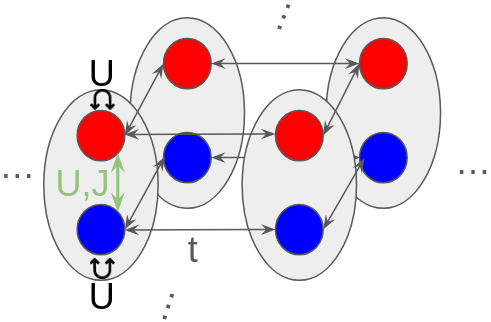
Figure 1: Pictorial view of the prototypical two-orbital Hubbard model considered in this work.

3 Benchmarking

Before benchmarking the approaches numerically, we will try to provide an analytical understanding of when the approach is suitable and when it it not. The model utilized in these benchmarks are variations of a multi-orbital Hubbard model, where each site contains two orbitals, see Fig. 1. If not mentioned otherwise, the two orbitals are not kinetically coupled and we set $t=1$ and give all other quantities relative to $t$. Furthermore, the orbitals have a coupling on the two-particle level due to the Hubbard-Kanamori interaction, which is parameterized by the on-site interaction $U$ and the Hunds coupling $J$. Such a model and its variations have been studied extensively in former works [90, 19, 95], to which we will compare our results. To analyze this model analytically, we consider two extreme cases, the one in which no Hunds coupling is present and the case in which the Hunds-coupling is $U/3$.

3.1 Model with pure density-density interactions

First, let us consider the case of a multi-orbital model with density-density interactions only. For the kinetic part of the Hamiltonian we consider a two-orbital square-lattice model without hopping between the orbitals,

$$H_{kin}=\sum_{\braket{i,j},o_{1},o_{2},s}tc^{\dagger}_{i,o_{1},s}c_{j,o_{2},s}\;,$$ (47)

where $i,j$ label the lattice sites. We furthermore assume half-filling. Due to the absence of inter-orbital hoppings the non-interacting susceptibility has a block diagonal form:

$$\chi^{0}_{o_{1},o_{4},o_{2},o_{3}}(q,\omega)=G_{o_{1}o_{4}}(k,\nu)G_{o_{2}o_{3}}(k-q,\nu-\omega)=\delta_{o_{1},o_{4}}\delta_{o_{2},o_{3}}\chi^{0}(q,\omega)\,,$$ (48)

where $\chi^{0}(q,\omega)$ is the susceptibility of the single band model. In this model we assume a pure density-density type interaction (meaning zero Hund’s coupling $J$)

$${H}_{\text{int}}=\sum_{i,o_{1},o_{2},s}Un_{i,o_{1},s}n_{i,o_{2},\bar{s}}+(1-\delta_{o_{1}o_{2}})Un_{i,o_{1},s}n_{i,o_{2},{s}}\;.$$ (49)

This interaction in combination with the kinetic term leads to a vanishing $\Sigma^{0}$, so that we do not have to consider it in the following. Since $J=0$ there is no spin selectivity and we thus expect $\braket{n_{0}^{\uparrow}n_{1}^{\uparrow}}=\braket{n_{0}^{\uparrow}n_{1}^{\downarrow}}$. Further, since $U=U^{\prime}$ there is no energy difference in double occupying the same or different orbitals, and hence $\braket{n_{0}^{\uparrow}n_{1}^{\downarrow}}=\braket{n_{0}^{\uparrow}n_{0}^{\downarrow}}$. This also implies that the double occupancy $\braket{n_{0}^{\uparrow}n_{0}^{\downarrow}}$ should decrease less rapidly with $U$ than for $U^{\prime}=0$. With this in mind we now turn to TPSC.

For a pure density-density interaction, the only non-zero Ansatz (TPSC3 and TPSC5 are giving identical results in this specific case, so we discuss TPSC3 here) is the one for $\tilde{D}$:

$$\tilde{D}_{o_{4},o_{1}} =D_{o_{4},o_{1}}\frac{\sum_{s_{4}}\bar{\delta}_{s_{1},s_{4}}^{o_{1},o_{4}}\braket{n_{o_{4}}^{s_{4}}n_{o_{1}}^{s_{1}}}}{\sum_{s_{4}}n_{o_{4}}^{s_{4}}n_{o_{1}}^{s_{1}}-n_{o_{1}o_{4}}^{s_{1}s_{4}}n_{o_{4}o_{1}}^{s_{4}s_{1}}}\,.$$ (50)

As we are at half-filling and have no inter-orbital coupling the denominator simplifies to

$$0.5-0.25\delta_{o_{1},o_{4}}\;.$$ (51)

The numerator is obtained via the Ansatz equations and thereby via the interacting susceptibility. Inserting the explicit form of the vertex derived from the Ansatz, as well as the non-interacting susceptibility, we arrive at

$$\chi_{o_{1},o_{2},o_{3},o_{4}}(q,\omega) =\sum_{o_{1}^{\prime},o_{3}^{\prime}}\delta_{o_{1},o_{4}}\delta_{o_{2}^{\prime},o_{3}^{\prime}}\chi^{0}(q,\omega)$$ (52)

$$\;\left(\frac{1}{{I}_{a^{\prime}b^{\prime}}\delta_{a^{\prime},d^{\prime}}\delta_{b^{\prime},c^{\prime}}-\delta_{a^{\prime},d^{\prime}}\delta_{e^{\prime},f^{\prime}}\chi^{0}(q,\omega)\tilde{U}\delta_{e^{\prime},f^{\prime}}\delta_{b^{\prime},c^{\prime}}}\right)_{o_{1}^{\prime},o_{2},o_{3},o_{4}^{\prime}}$$

$$=\delta_{o_{1},o_{4}}\delta_{o_{2},o_{3}}\chi^{0}(q,\omega)\frac{1}{1-\chi^{0}(q,\omega)\tilde{U}}\,,$$ (53)

where the fraction in the first line denotes a matrix inversion.

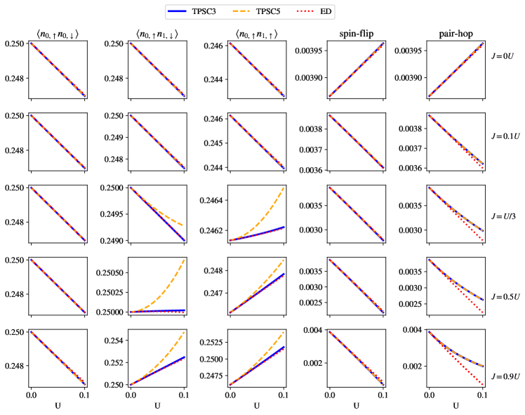
Figure 2: Comparison between TPSC3 (blue), TPSC5 (yellow) and ED (red) for the model defined in Eq. (54) at $\beta=0.5$, for different $U$ and $J$ combinations. We include the zeroth order self-energy in both TPSC variants.

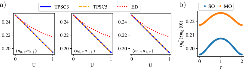
Figure 3: (a) Comparison between TPSC and ED at $\beta=2$ for different $U$ at $J=0$. We observe the same phenomenology as expected from our analytical analysis. (b) Time dependence of the density-density correlator for a single (SO) and a two-orbital (MO) two-site Hubbard model. No enhancement of the time dependence is visible, and hence this cannot explain the larger deviation to DMFT in the multi-orbital case.

We note that the interacting susceptibility is identical to the one of a single orbital model with the same interaction value. The only non-zero components of the susceptibility are $\chi_{1111}$ and $\chi_{1221}$. Thus, from Eq. (40) and Eq. (41) it immediately follows that $\braket{n_{0}^{\uparrow}n_{1}^{\uparrow}}=\braket{n_{0}^{\uparrow}n_{1}^{\downarrow}}=\braket{n_{0}^{\uparrow}n_{0}^{\downarrow}}$, as we expected from the arguments above. In contrast to our expectations, the specific form of the susceptibility implies that the converged TPSC loop will result in the same double occupancy as the one for the one-orbital model. In other words, adding an inter-orbital interaction of the same strength as the bare interaction does not make a difference for the double occupation predicted by the method. This is in contrast to the physically expected result discussed above – in the single orbital model in the strong coupling limit, we would expect zero double occupancy. However in this model, different states in which no orbital is doubly occupied and states in which all orbitals are doubly occupied are degenerate in energy so the double occupancy should decay much slower (as it is seen in ED, see Fig. 3a).

To pinpoint what TPSC is missing in this case, we consider two coupled dimers (2-site) for which we compare the results between ED and TPSC. The behavior described above is reproduced as expected, see Fig. 3a. Further, since the susceptibility does not gain any strong $\tau$ dependence, implying that the frequency dependence also does not change drastically, as shown in Fig. 3b, we expect the vertex to be still reasonably well described by the static limit. The questions therefore are, first, where does the deviation stem from and second, why does this issue occur here but not in the single orbital model?

Let us first answer the second question. In the single-orbital case we fix the local and static expectation value to be the exact one. Crucially, the single site contains no further internal structure meaning that the exact local expectation value is always proportional to the non-interacting one. Thus representing this expectation value locally by a renormalized Hartree-Fock expectation value works, i.e., we can always get the correct value of the double occupancy by multiplying the non-interacting double occupancy with a single number. Multi-orbital systems have additional degrees of freedom, which enter the local and static contribution. We still approximate the TPEVs in a Hartree-Fock fashion, thus as a single Slater-determinant which intrinsically is connected to the non-interacting limit. Importantly, the local Hilbert-space is now spanned by more than a single wave-function and all of these states contribute to the expectation value. Thus, introducing interactions can fundamentally alter the structure of the eigenstates in the local Hamiltonian, so that the expectation value can deviate from a behavior representable by the non-interacting one. As an illustration, let us considering a dimer at half-filling with a Hubbard-Kanamori interaction. At $t=0$ all $S=1$ states are degenerate producing vastly different TPEV’s. In TPSC only one of these three states is represented by the Hartree-Fock decoupling and the others are missed entirely (thus behaving like the single orbital model in the absence of $J$). Thereby the basic idea of TPSC, which relies on fixing the local and static expectation values, breaks down. Further, this immediately suggests that the issue arises due to the Hartree-Fock decoupling, which is central to TPSC and thus there is no fix to this problem without altering the structure of the method.

3.2 Analysis of the model with $J=U/3$

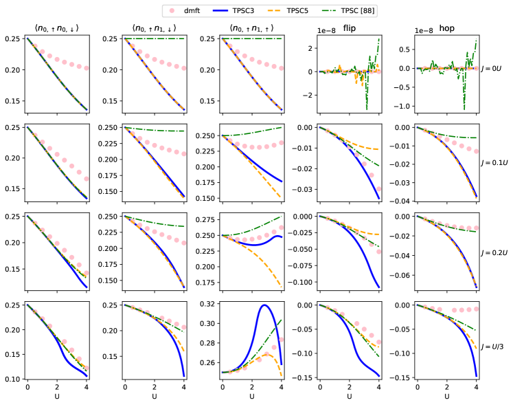
Figure 4: Comparison between density-density correlations obtained with TPSC3 (green), TPSC5 (red), TPSC from Ref. [90] (blue) and DMFT (pink dots) for the two-orbital Hubbard model defined in Eq. (56) at $\beta=2$, for different $U$ and $J$ values.

If $J=U/3$, the same-spin density-density interaction becomes exactly zero. This choice is interesting, as it is the limiting case where the approach in Ref. [90] and TPSC resulted in the best agreement compared to DMFT, as is shown in Fig. 4. What is the origin of this apparent improvement? First, we should note that this is not a magic value at which the approach suddenly works, but there appears to be a steady improvement with increasing $J$. Second, we observe that for $J=U/3$ the same-spin interaction is exactly $0$ and stays at that value throughout the calculation in TPSC5. In TPSC3 this interaction will gain a nonzero value, leading to the instability we observe in Fig. 4.

Since we are again mainly interested in the quality of the TPEV’s predicted from the spin sum rules, for now let us consider the half-filled dimer, a single unit cell of the form sketched in Fig. 1. In this toy model, the spectrum consists of three groups; the $S=1$ group with eigenvalue $U-3J$ and the $S=0$ group which is split into a two-fold degenerate pair at $U-J$ and a single eigenvalue with $U+J$. Thus, while the point $U=3J$ is not special, the separation between the excited state and the ground state grows linearly with $J$. Furthermore, the $S=1$ subspace is kind of special, as two states only contribute to a single TPEV ($\braket{n^{\uparrow}_{0}n^{\uparrow}_{1}}$) and the other state essentially behaves like in the single orbital model. Therefore, one should be able to approximate the TPEV’s by a scaling in all components but the $\braket{n^{\uparrow}_{0}n^{\uparrow}_{1}}$ one, which is incorrectly estimated because of the missing degenerate states. This is exactly what is observed for both TPSC5 and in Ref. [90]. Thus we conclude that in the end this improvement is related to the structure and number of states determining the local and static expectation values.

From these observations, we can extract a guiding principle of when to expect TPSC to work in a multi-orbital setting and when not. If there is a gap in the local spectrum between the ground state and the excited states, TPSC should perform better than when the states are close in energy. Further, when analyzing the nature of the states, we can extract which TPEV is expected to deviate strongly and which not. This also indicates that this specific part of TPSC performs better at lower temperatures (since it is basically a ground state targeting approach) - however, the local and static approximation of the vertex becomes more and more inappropriate at lower temperatures which is why TPSC typically fails at low temperatures.

In summary, the regimes in which multi-orbital TPSC is guaranteed to work well are the weak coupling limit and a small region in which excited states do not contribute to the local TPEVs (controlled by temperature and the gap), while the vertex still is local and static. The former is accessible by inspection, while the latter one is not clear a priori and requires other numerical simulations to be fully gauged. Notably, the issue described above is partially resolved when starting from DMFT TPEVs [91, 95].

3.3 Numerical benchmarks

Keeping the above described shortcomings in mind, we are now exploring the range of applicability of multi-orbital TPSC by testing the reliability of TPSC3 and TPSC5 through comparison to more accurate numerical approaches. In a first step, we exclusively aim at validating the quality of the predicted TPEVs, as these form the basis for the TPSC approach. For this we compare to both ED and DMFT.

3.3.1 Comparison to ED

First, we compare the predicted TPEV between ED an TPSC, for a two-orbital dimer with Hubbard-Kanamori interactions

$$H=\sum_{\sigma}t(c^{\dagger}_{0,s^{\prime}}c_{1,s^{\prime}}+c^{\dagger}_{1,s^{\prime}}c_{0,s^{\prime}})+H^{HK}\,,$$ (54)

where we introduced a Hubbard-Kanamori type interaction given as

$$H^{HK}=U\hat{n}_{o_{1}^{\prime}}^{\uparrow}\hat{n}_{o_{1}^{\prime}}^{\downarrow}+\sum_{{o_{1}^{\prime}}\neq{o_{2}^{\prime}}} \left((U-2J)\hat{n}_{o_{1}^{\prime}}^{\uparrow}\hat{n}_{o_{2}^{\prime}}^{\downarrow}+(U-3J)\hat{n}_{o_{1}^{\prime}}^{s^{\prime}}\hat{n}_{o_{2}^{\prime}}^{s^{\prime}}\right.$$ (55)

$$\quad\left.-J\hat{c}^{{\dagger}}_{o_{1}^{\prime},\uparrow}\hat{c}_{o_{1}^{\prime},\downarrow}\hat{c}^{{\dagger}}_{o_{2}^{\prime},\downarrow}\hat{c}_{o_{2}^{\prime},\uparrow}+J\hat{c}^{{\dagger}}_{o_{1}^{\prime},\uparrow}\hat{c}^{{\dagger}}_{o_{1}^{\prime},\downarrow}\hat{c}_{o_{2}^{\prime},\downarrow}\hat{c}_{o_{2}^{\prime},\uparrow}\right)\,.$$

Here $U$ and $J$ are measured in units of $t$ which is set to $1$. We consider weak coupling where the TPSC formalism should give the correct leading order behavior. For the ED calculations, we use pyED [108] from the TRIQS framework [109]. The results for all three methods as a function of $U$ and $J$ are plotted in Fig. 2.

Both TPSC3 and TPSC5 show indeed the correct leading order behavior for all TPEVs, irrespective of the ratio of $U$ and $J$. Further, we observe that TPSC5 performs significantly worse when $J$ becomes unphysically large, while TPSC3 stays much closer to the ED result. This trend also persists at lower temperatures, see Fig. 7 in Appendix B. The TPEV do match well between TPSC3 and ED throughout the whole range of examined parameters. In general, the deviation is strongest in the pair-hopping component, in which the error monotonously increases with $J$. We stress again that since we stay in the weak-coupling regime, these benchmarks have no direct implications for applications in the strongly correlated regime.

3.3.2 Comparison to DMFT

As a next step, we compare the results from TPSC to DMFT. For this, we consider the same model as Ref. [90]

$$\hat{H}=\sum_{s,\braket{i,j},o}tc^{\dagger}_{o,s,i}c^{\dagger}_{o,s,j}+\hat{H}_{HK}\,,$$ (56)

where $t=1$ is fixed and the inverse temperature is $\beta=2$. For completeness, we include the results from the implementation proposed in Ref. [90] (here named TPSC). The DMFT calculations are performed using w2dynamics [64].

This model can be seen as a worst-case scenario as in the absence of inter-orbital hopping the off-diagonal occupations are guaranteed to be zero. Hence, the $P$-channel as well as opposite spin $C$-channel (in the case of TPSC5) Ansatz equations are ill-defined, making a renormalization of the corresponding vertices impossible. In other words, the corresponding Hartree-Fock decouplings always result in a net-zero contribution of these terms to the self-energy. Interestingly, even though the Ansatz equations might break down, the derivation remains valid – we can still renormalize these components, albeit in a less controlled fashion. We found that fixing the renormalization of the channels to that of the one channel in which the Ansatz is not ill-defined works for a wide range of parameters.

Both proposed TPSC approaches show promising results in the weak-coupling regime, but the deviation from DMFT rapidly increases with stronger interactions. Assuming that the DMFT results are accurate, the error is largest in the absence of Hund’s coupling and becomes smaller for larger $J$, as expected from our discussion above. In general TPSC5 seems to outperform TPSC3, even though both fulfill the internal consistency check in the small to intermediate coupling region. Notably, there is no significant improvement in the case of large Hund’s couplings when compared to the approach put forward in Ref. [90].

3.4 Comparison of interacting susceptibilities

In addition to the quality of the TPEV’s we can also test the interacting charge and spin susceptibilities. In the following we will compare our results to D-TRILEX [19], again for a model of the form of Fig. 1, however introducing a hopping imbalance between the red and blue orbitals

$$H=\sum_{\alpha,\braket{i,j},s}t_{\alpha}c^{\dagger}_{\alpha,s,i}c_{\alpha,s,j}+H_{HK}$$ (57)

with $t_{\mathrm{red}}=1$ and $t_{\mathrm{blue}}=0.75$. $U$ and $J$ are in the following given in units of $t_{\mathrm{red}}$.

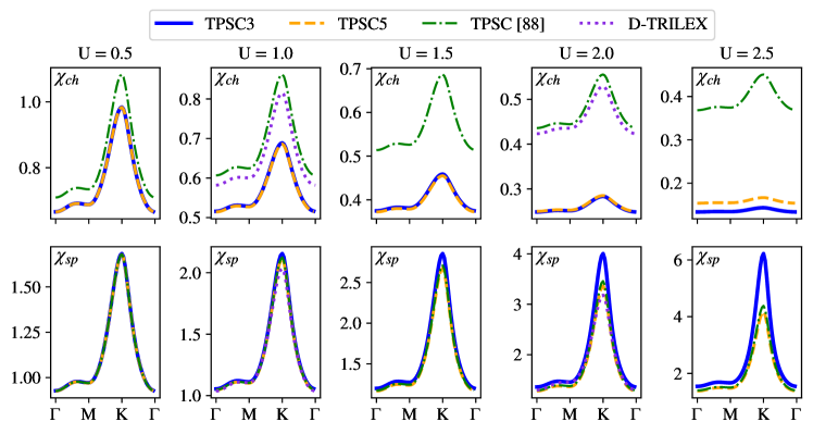
Figure 5: Comparison of the charge (upper row) and spin (lower row) susceptibility between TPSC3 (blue), TPSC5 (orange), TPSC from Ref. [66] (green) and D-TRILEX (purple) at different $U$ and $J=0.2U$ at $\beta=2$.

We find that both TPSC algorithms over/underestimate the spin/charge susceptibility in comparison to D-TRILEX, which was also found in Ref [95]. However, the overestimation is weaker for TPSC5 and stronger for TPSC3. Most notably, the charge susceptibility is even stronger suppressed than in prior TPSC formulations.

4 Conclusion and Outlook

In this paper we introduced two variants of a fully self-consistent multi-orbital TPSC approach dubbed TPSC3 and TPSC5. We analyzed the structure of the equations and showed analytically that in the limit of vanishing Hund’s coupling the Ansatz equations result in the same TPEVs as for the single orbital model, which is unphysical. Further, we provided an explanation for this behavior in terms of the equivalence between the Hatree-Fock decomposition and a minimization in terms of single Slater determinants, highlighting that representing influences from many low energy states onto the TPEVs are not fully reproducible by a single state with modified prefactors. Furthermore, by considering the local Hilbert space we provided an understanding of why the approach performs better at larger $J/U$. Notably, this understanding allows to assess the expected quality of the results from TPSC by inspecting the local spectrum. On a qualitative level, we found that the TPEVs from TPSC5 outperform the ones from TPSC3 when compared to DMFT. Furthermore, in the limiting case of $J=U/3$ the new variants do not outperform the conceptually simpler but approximate approach suggested in Ref. [90].

While TPSC itself cannot be improved much without fundamentally modifying the basic approach, the recently proposed combination of TPSC and DMFT [95, 91] resolves partially the issue of wrong TPEVs due to the Hartree-Fock decoupling but also ensures the correct handling of correlations at the zeroth-order level. Thus, in multi-orbital systems, the application of TPSC in combination DMFT appears as the most promising route to correct for the flaws uncovered in the present work and in Ref. [91]. A major advantage of TPSC in this formulation is that no vertex needs to be extracted from the DMFT simulation, which offers a numerically much cheaper alternative to D-TRILEX and related approaches [14, 19].

5 Acknowledgements

The authors are grateful to A. Razpopov, P. P. Stavropoulos, L. Klebl and G. Rohringer for valuable discussions and E. Stepanov for providing the reference data from D-TRILEX. We acknowledge support by the Deutsche Forschungsgemeinschaft (DFG, German Research Foundation) for funding through project QUAST-FOR5249 - 449872909 (project TP4) and (project TP6). J.Y. and P.W. also acknowledge support from SNSF Grant No. 200021-196966.

Appendix A Kadanoff-Baym Formalism

In the following we derive the central equations for the multi-orbital TPSC approach, following Ref. [80, 90]. Our starting point is the Green’s function generating functional [110]

$$\mathcal{G}[\phi]=-\ln\langle T_{\tau}e^{-c^{\dagger}_{1^{\prime}}c_{2^{\prime}}\phi_{1^{\prime},2^{\prime}}}\rangle=-\ln\langle T_{\tau}S[\phi]\rangle=\ln(Z[\phi])\,.$$ (58)

We use numbers as a short hand for a collection of spin, orbital, position and time indices. Primed variables are summed over. The external source field $\phi$ has been introduced as a mathematical trick and at the end of the calulation it can be set to $0$. The single particle Green’s function is obtained as the functional derivative of $\mathcal{G}$ with respect to $\phi$

$$G_{1,2;\phi}=\frac{\delta\mathcal{G}}{\delta\phi(2,1)}=-\frac{\braket{T_{\tau}S[\phi]c_{1}c^{\dagger}_{2}}}{Z[\phi]}\,.$$ (59)

With this, we perform a Legendre transformation giving us the vertex generating functional or Luttinger-Ward functional $\Phi[G]$ whose first derivative is the self-energy

$$\Sigma_{1,2;\phi}=-\frac{\delta\Phi[G]}{\delta G(2,1)}\,.$$ (60)

From the Legendre transform relation between the generating functionals the Dyson-equation follows as

$$G^{-1}=G_{0}^{-1}-\phi-\Sigma\,.$$ (61)

The second functional derivative of $\mathcal{G}[\phi]$ is the generalized susceptibility given as

$$\chi_{1423}=\frac{\delta G_{1,2;\phi}}{\delta\phi_{3,4}}=\braket{c_{1}c^{\dagger}_{2}c^{\dagger}_{3}c_{4}}_{\phi}+\braket{c_{1}c^{\dagger}_{2}}_{\phi}\braket{c_{4}c^{\dagger}_{3}}_{\phi}\,,$$ (62)

while the vertex can be expressed as

$$\Gamma_{1,2,3,4}=\frac{\delta\Sigma_{1,2}}{\delta G_{3,4}}\,.$$ (63)

With these we obtain a Dyson-equation like connection between the interacting and non-interacting susceptibility:

$$0 =\frac{\delta(G^{-1}_{1,3^{\prime}}G_{3^{\prime},3})}{\delta{\phi_{4,2}}}$$ (64)

$$=G^{-1}_{1,3^{\prime}}\frac{\delta(G_{3^{\prime},3})}{\delta{\phi_{4,2}}}+\frac{\delta(G^{-1;0}_{1,3^{\prime}}-\phi_{1,3^{\prime}}-\Sigma_{1,3^{\prime}})}{\delta{\phi_{4,2}}}G_{3^{\prime},3}$$ (65)

$$\Leftrightarrow\chi_{1,2,3,4} =-G_{1,1^{\prime}}\frac{(\delta\phi_{1^{\prime},3^{\prime}}+\Sigma_{1^{\prime},3^{\prime}})}{\delta{\phi_{4,2}}}G_{3^{\prime},3}$$ (66)

$$=\chi^{0}_{1,2,3,4}-G_{1,1^{\prime}}\frac{\delta\Sigma_{1^{\prime},3^{\prime}}}{\delta{G_{4^{\prime},2^{\prime}}}}\frac{\delta G_{4^{\prime},2^{\prime}}}{\delta{\phi_{4,2}}}G_{3^{\prime},3}$$ (67)

$$=\chi^{0}_{1,2,3,4}+\chi^{0}_{1,3^{\prime},3,1^{\prime}}\Gamma_{1^{\prime},3^{\prime},4^{\prime},2^{\prime}}\chi_{4^{\prime},2,2^{\prime},4}\,,$$ (68)

which is the general form of the Bethe-Salpeter equation. In a $SU(2)$ symmetric system, we can further use that all occuring quantities are diagonal in physical spin-space, thus resulting in spin-channel-specific equations which read (pulling out spin indices from the numbers)

$$\chi^{S^{i^{\prime}},S^{j^{\prime}}}_{1,2,3,4} =(\chi^{0}_{1,2,3,4}+\chi^{0}_{1,3^{\prime},3,1^{\prime}}\Gamma_{1^{\prime},3^{\prime},4^{\prime},2^{\prime}}\chi_{4^{\prime},2,2^{\prime},4})\sigma^{i}_{s_{1},s_{3}}\sigma^{j}_{s_{2},s_{4}}$$ (69)

$$\Leftrightarrow\chi_{1,2,3,4}^{S^{z},S^{z}} =\chi_{1,2,3,4}^{0;S^{z},S^{z}}+\chi^{0;S^{z},S^{z}}_{1,3^{\prime},3,1^{\prime}}\Gamma_{1^{\prime},3^{\prime},4^{\prime},2^{\prime}}^{S^{z},S^{z}}\chi_{4^{\prime},2,2^{\prime},4}^{S^{z},S^{z}}$$ (70)

$$\Leftrightarrow\chi_{1,2,3,4}^{S^{0},S^{0}} =\chi_{1,2,3,4}^{0;S^{0},S^{0}}-\chi^{0;S^{0},S^{0}}_{1,3^{\prime},3,1^{\prime}}\Gamma_{1^{\prime},3^{\prime},4^{\prime},2^{\prime}}^{S^{0},S^{0}}\chi_{4^{\prime},2,2^{\prime},4}^{S^{0},S^{0}}\,,$$ (71)

where $S_{x}S_{x}$, $S_{y}S_{y}$ and $S_{z}S_{z}$ are related by $SU(2)$ symmetry.

The equation of motion is a central building block for TPSC, and for completeness we derive it here for a Hamiltonian with local and static two-electron interactions,

$$H=t_{13}c^{\dagger}_{3}(\tau)c_{1}(\tau)+\frac{1}{2}U_{1234}c^{\dagger}_{3}(\tau)c^{\dagger}_{4}(\tau)c_{2}(\tau)c_{1}(\tau)\,.$$ (72)

In this case, the Heisenberg equation of motion reads

$$\partial_{\tau_{5}}c_{5}(\tau_{5}) =\left[H,c_{5}(\tau_{5})\right]$$ (73)

$$=\left[t_{1^{\prime}3^{\prime}}c^{\dagger}_{3^{\prime}}(\tau)c_{1^{\prime}}(\tau),c_{5}(\tau_{5})\right]+\frac{1}{2}\left[U_{1^{\prime}2^{\prime}3^{\prime}4^{\prime}}c^{\dagger}_{3^{\prime}}(\tau)c^{\dagger}_{4^{\prime}}(\tau)c_{2^{\prime}}(\tau)c_{1^{\prime}}(\tau),c_{5}(\tau_{5})\right]$$ (74)

$$=-t_{1^{\prime}3^{\prime}}\{c_{3^{\prime}}^{\dagger},c_{5}(\tau_{5})\}c_{1^{\prime}}+\frac{1}{2}U_{1^{\prime}2^{\prime}3^{\prime}4^{\prime}}\left(c_{3^{\prime}}^{\dagger}(\tau)c_{4^{\prime}}^{\dagger}(\tau)\{c_{2^{\prime}}(\tau)c_{1^{\prime}}(\tau),c_{5}(\tau_{5})\}\right.$$ (75)

$$\quad\quad\quad-\left.\{c_{3^{\prime}}^{\dagger}(\tau)c_{4^{\prime}}^{\dagger}(\tau),c_{5}(\tau_{5})\}c_{2^{\prime}}(\tau)c_{1^{\prime}}(\tau)\right)$$ (76)

$$=-t_{1^{\prime}3^{\prime}}c_{1^{\prime}}(\tau_{5})\delta_{3^{\prime},5}+\frac{1}{2}U_{1^{\prime}2^{\prime}3^{\prime}4^{\prime}}\left(c_{3^{\prime}}^{\dagger}(\tau)\delta_{5,4^{\prime}}-\delta_{5,3^{\prime}}c_{4^{\prime}}^{\dagger}(\tau)\right)\delta_{\tau,\tau_{5}}c_{2^{\prime}}(\tau)c_{1^{\prime}}(\tau)$$ (77)

$$=-t_{1^{\prime}3^{\prime}}c_{1^{\prime}}(\tau_{5})\delta_{3^{\prime},5}+U_{1^{\prime}2^{\prime}3^{\prime}4^{\prime}}c_{3^{\prime}}^{\dagger}(\tau_{5})\delta_{4^{\prime},5}c_{2^{\prime}}(\tau_{5})c_{1^{\prime}}(\tau_{5})\,,$$ (78)

where we exploited the crossing symmetry of $U$ and relabeled the summation indices in the last line. From this we find the equation of motion for the Green’s function as

$$\partial_{\tau_{a}}G_{a,b,\phi}(\tau_{a},\tau_{b})= \phi_{a1^{\prime}}G_{1^{\prime}b}(\tau_{1}^{\prime},\tau_{b})+\delta_{a,b}-t_{1a}\braket{c_{1}(\tau_{a})c^{\dagger}_{b}(\tau_{b})}$$ (79)

$$+U_{1^{\prime}2^{\prime}3^{\prime}a}\braket{c_{3^{\prime}}^{\dagger}(\tau_{a})c_{2^{\prime}}(\tau)c_{1^{\prime}}(\tau_{a})c^{\dagger}_{b}(\tau_{b})}\,.$$

By comparing with the Schwinger Dyson equation we extract

$$\Sigma_{1,1^{\prime}}(\tau_{1},\tau_{1}^{\prime})G_{1^{\prime},3}(\tau_{1}^{\prime},\tau_{3})=U_{4^{\prime},2^{\prime},5^{\prime},1}\braket{c_{5^{\prime}}^{\dagger}(\tau_{1})c_{2^{\prime}}(\tau_{1})c_{4^{\prime}}(\tau_{1})c^{\dagger}_{3}(\tau_{3})}\,,$$ (80)

which is the central equation for all following derivations. Note that we could have analogously taken the initial derivative w.r.t $\tau_{b}$ which would result in

$$\Sigma_{1,1^{\prime}}(\tau_{1},\tau_{1}^{\prime})G_{1^{\prime},3}(\tau_{1}^{\prime},\tau_{3})=U_{4^{\prime},2^{\prime},5^{\prime},1}\braket{c_{5^{\prime}}^{\dagger}(\tau_{3})c_{2^{\prime}}(\tau_{3})c_{4^{\prime}}(\tau_{1})c^{\dagger}_{3}(\tau_{3})}\,.$$ (81)

A.1 Self-energy

We can re-express the implicit equation for the self-energy as an explicit one, the Schwinger-Dyson equation:

$$\Sigma_{1,1^{\prime}}(\tau_{1},\tau_{1}^{\prime})G_{1^{\prime},3} (\tau_{1}^{\prime},\tau_{3})=U_{4^{\prime},2^{\prime},5^{\prime},1}\braket{c_{5^{\prime}}^{\dagger}(\tau_{1})c_{2^{\prime}}(\tau_{1})c_{4^{\prime}}(\tau_{1})c^{\dagger}_{3}(\tau_{3})}$$ (82)

$$=U_{4^{\prime},2^{\prime},5^{\prime},1}\left(\chi_{2^{\prime},4^{\prime},5^{\prime},3}(\tau_{1},\tau_{1},\tau_{1},\tau_{3})-G_{2^{\prime},5^{\prime}}(\tau_{1},\tau_{1})G_{4^{\prime},3}(\tau_{1},\tau_{3})\right)$$ (83)

$$=U_{4^{\prime},2^{\prime},5^{\prime},1}\Big{(}\chi_{2^{\prime},a^{\prime},5^{\prime},b^{\prime}}(\tau_{1},\tau_{5},\tau_{1},\tau_{5})\Gamma_{b^{\prime},a^{\prime},c^{\prime},d^{\prime}}\ G_{c^{\prime},3}(\tau_{5}\tau_{3})G_{4^{\prime},d^{\prime}}(\tau_{1},\tau_{5})$$ (84)

$$\quad+G_{2^{\prime},3}(\tau_{1},\tau_{3})G_{4^{\prime},5^{\prime}}(\tau_{1},\tau_{1})-G_{2^{\prime},5^{\prime}}(\tau_{1},\tau_{1})G_{4^{\prime},3}(\tau_{1},\tau_{3})\Big{)}$$

$$\Leftrightarrow\Sigma_{1,5}(\tau_{1},\tau_{5}) =U_{4^{\prime},2^{\prime},5^{\prime},1}\Big{(}\chi_{2^{\prime},a^{\prime},5^{\prime},b^{\prime}}(\tau_{1},\tau_{5},\tau_{1},\tau_{5})\Gamma_{b^{\prime}a^{\prime}5d^{\prime}}\ G_{4^{\prime},d^{\prime}}(\tau_{1},\tau_{5})$$ (85)

$$\quad+2G_{4^{\prime},5^{\prime}}(\tau_{1},\tau_{1})\delta_{2^{\prime},5}\delta_{\tau_{1},\tau_{5}}\Big{)}\,.$$

Here, the latter term corresponds to the Hartree-Fock selfenergy, while the former is the Schwinger-Dyson equation. At this point, we are working in diagrammatic spin-space. However, the susceptibility and the vertex are only known in the physical spin-space. Furthermore, we can utilize that the self-energy and Green’s function are spin diagonal. Hence, we pull the spin-dependence out of the combined index

$$\Sigma_{1,5} (\tau_{1},\tau_{5})\delta_{s_{1},s_{5}}=(U_{4^{\prime},2^{\prime},5^{\prime},1}\delta_{s_{4}^{\prime},s_{5}^{\prime}}\delta_{s_{2}^{\prime},s_{1}}-U_{4^{\prime}2^{\prime}15^{\prime}}\delta_{s_{4}^{\prime},s_{1}}\delta_{s_{2}^{\prime},s_{5}^{\prime}})$$ (86)

$$\quad\Big{(}\frac{1}{4}S^{i^{\prime}}_{s_{2}^{\prime},s_{5}^{\prime}}S^{i^{\prime}}_{\sigma_{a}^{\prime},\sigma_{b}^{\prime}}\chi^{S^{i^{\prime}}S^{i^{\prime}}}_{2^{\prime},a^{\prime},5^{\prime},b^{\prime}}(\tau_{1},\tau_{5},\tau_{1},\tau_{5})S^{j^{\prime}}_{\sigma_{b}^{\prime},\sigma_{a}^{\prime}}S^{j^{\prime}}_{s_{5},\sigma_{d}^{\prime}}\Gamma^{S^{j^{\prime}}S^{j^{\prime}}}_{b^{\prime}a^{\prime}5d^{\prime}}G_{4^{\prime},d^{\prime}}(\tau_{1},\tau_{5})\delta_{s_{4}^{\prime},\sigma_{d}^{\prime}}$$

$$\quad+\delta_{2^{\prime},5}\delta_{\tau_{1},\tau_{5}}G_{4^{\prime},5^{\prime}}(\tau_{1},\tau_{1})\delta_{s_{4}^{\prime},s_{5}^{\prime}}-G_{2^{\prime},5^{\prime}}(\tau_{1},\tau_{1})\delta_{4^{\prime},5}\delta_{\tau_{1},\tau_{5}}\delta_{s_{2}^{\prime},s_{5}^{\prime}}\Big{)}$$

$$=2U_{4^{\prime},2^{\prime},5^{\prime},1}G_{4^{\prime},5^{\prime}}(\tau_{1},\tau_{1})\delta_{2^{\prime},5}\delta_{\tau_{1},\tau_{5}}-U_{4^{\prime}2^{\prime}15^{\prime}}G_{4^{\prime},5^{\prime}}(\tau_{1},\tau_{1})\delta_{2^{\prime},5}\delta_{\tau_{1},\tau_{5}}$$ (87)

$$\quad+\frac{1}{4}U_{4^{\prime},2^{\prime},5^{\prime},1}G_{4^{\prime},d^{\prime}}(\tau_{1},\tau_{5})\chi^{S^{i^{\prime}}S^{i^{\prime}}}_{2^{\prime},a^{\prime},5^{\prime},b^{\prime}}(\tau_{1},\tau_{5},\tau_{1},\tau_{5})\Gamma^{S^{j^{\prime}}S^{j^{\prime}}}_{b^{\prime}a^{\prime}5d^{\prime}}S^{i^{\prime}}_{s_{1},\sigma_{d}^{\prime}}S^{i^{\prime}}_{\sigma_{a}^{\prime},\sigma_{b}^{\prime}}S^{j^{\prime}}_{\sigma_{b}^{\prime},\sigma_{a}^{\prime}}S^{j^{\prime}}_{s_{5},\sigma_{d}^{\prime}}$$

$$\quad-\frac{1}{4}U_{4^{\prime}2^{\prime}15^{\prime}}G_{4^{\prime},d^{\prime}}(\tau_{1},\tau_{5})\chi^{S^{i^{\prime}}S^{i^{\prime}}}_{2^{\prime},a^{\prime},5^{\prime},b^{\prime}}(\tau_{1},\tau_{5},\tau_{1},\tau_{5})\Gamma^{S^{j^{\prime}}S^{j^{\prime}}}_{b^{\prime}a^{\prime}5d^{\prime}}S^{i^{\prime}}_{s_{5}^{\prime},s_{5}^{\prime}}\delta_{i^{\prime},j^{\prime}}2S^{j^{\prime}}_{s_{5},s_{1}}$$

$$=2U_{4^{\prime},2^{\prime},5^{\prime},1}G_{4^{\prime},5^{\prime}}(\tau_{1},\tau_{1})\delta_{2^{\prime},5}\delta_{\tau_{1},\tau_{5}}-U_{4^{\prime}2^{\prime}15^{\prime}}G_{4^{\prime},5^{\prime}}(\tau_{1},\tau_{1})\delta_{2^{\prime},5}\delta_{\tau_{1},\tau_{5}}$$ (88)

$$\quad+U_{4^{\prime},2^{\prime},5^{\prime},1}G_{4^{\prime},d^{\prime}}(\tau_{1},\tau_{5})\chi^{S^{i^{\prime}}S^{i^{\prime}}}_{2^{\prime},a^{\prime},5^{\prime},b^{\prime}}(\tau_{1},\tau_{5},\tau_{1},\tau_{5})\Gamma^{S^{i^{\prime}}S^{i^{\prime}}}_{b^{\prime}a^{\prime}5d^{\prime}}$$

$$\quad-U_{4^{\prime}2^{\prime}15^{\prime}}G_{4^{\prime},d^{\prime}}(\tau_{1},\tau_{5})\chi^{S^{0}S^{0}}_{2^{\prime},a^{\prime},5^{\prime},b^{\prime}}(\tau_{1},\tau_{5},\tau_{1},\tau_{5})\Gamma^{S^{0}S^{0}}_{b^{\prime}a^{\prime}5d^{\prime}}$$

$$=(2U_{4^{\prime},5,5^{\prime},1}-U_{4^{\prime}515^{\prime}})G_{4^{\prime},5^{\prime}}(\tau_{1},\tau_{1})\delta_{\tau_{1},\tau_{5}}$$ (89)

$$\quad+3U_{4^{\prime},2^{\prime},5^{\prime},1}G_{4^{\prime},d^{\prime}}(\tau_{1},\tau_{5})\chi^{S^{z}S^{z}}_{2^{\prime},a^{\prime},5^{\prime},b^{\prime}}(\tau_{1},\tau_{5},\tau_{1},\tau_{5})\Gamma^{S^{z}S^{z}}_{b^{\prime}a^{\prime}5d^{\prime}}$$

$$\quad+(2U_{4^{\prime}2^{\prime}15^{\prime}}-U_{4^{\prime},2^{\prime},5^{\prime},1})G_{4^{\prime},d^{\prime}}(\tau_{1},\tau_{5})\chi^{S^{0}S^{0}}_{2^{\prime},a^{\prime},5^{\prime},b^{\prime}}(\tau_{1},\tau_{5},\tau_{1},\tau_{5})\Gamma^{S^{0}S^{0}}_{b^{\prime}a^{\prime}5d^{\prime}}\,.$$

There are two internal consistency checks - one for each flavor of TPSC, which is the usual internal consistency check between single and two-particle objects in the pairwise equal position, time and orbital limit:

$$\Sigma_{1,1^{\prime}}G_{1^{\prime},1} =\Big{(}D_{o_{4},o_{1}}\sum_{s_{4}}\bar{\delta}_{s_{1},s_{4}}^{o_{1},o_{4}}\braket{c_{o_{4},s_{4}}^{\dagger}c_{o_{1},s_{1}}c_{o_{4},s_{4}}c_{1}^{\dagger}}$$ (90)

$$\quad+C_{o_{1},o_{4}}\sum_{s_{4}}\bar{\delta}_{s_{1},s_{4}}^{o_{1},o_{4}}\braket{c_{o_{4},s_{4}}^{\dagger}c_{o_{4},s_{1}}c_{o_{1},s_{4}}c_{1}^{\dagger}}$$

$$\quad+\bar{\delta}_{s_{1},s_{4}}P_{o_{2},o_{1}}\sum_{s_{4}}\braket{c_{o_{1},s_{4}}^{\dagger}c_{o_{2},s_{1}}c_{o_{2},s_{4}}c_{1}^{\dagger}}\Big{)}.$$

Both TPSC3 and TPSC5 fulfill this up to numerical precision, as long as the self consistency loop for the spin channel TPEV’s and the subsequent TPEV fitting in the charge channel have a solution which is physical. A second consistency check is the equivalence between TPSC3 and TPSC5.

A.2 Zeroth order Self-energy

Within TPSC the Luttinger Ward functional for an $SU(2)$ symmetric model with local initial interactions is approximated as

$$\Phi[G] =\frac{1}{2}G_{o_{3}^{\prime},o_{1}^{\prime}}(r_{3}^{\prime},r_{1}^{\prime})\delta_{\sigma_{1}^{\prime}s_{3}^{\prime}}$$ (91)

$$\times(\Gamma_{o_{1}^{\prime}o_{2}^{\prime}o_{3}^{\prime}o_{4}^{\prime}}\delta_{\sigma_{1}^{\prime}s_{3}^{\prime}}\delta_{\sigma_{2}^{\prime}s_{4}^{\prime}}-\Gamma_{o_{1}^{\prime}o_{2}^{\prime}o_{4}^{\prime}o_{3}^{\prime}}\delta_{\sigma_{1}^{\prime}s_{4}^{\prime}}\delta_{\sigma_{2}^{\prime}s_{3}^{\prime}})\delta_{(r_{1}^{\prime},r_{2}^{\prime},r_{3}^{\prime},r_{4}^{\prime})}G_{o_{4}^{\prime},o_{2}^{\prime}}(-r_{4}^{\prime},r_{2}^{\prime})\delta_{\sigma_{2}^{\prime}s_{4}^{\prime}}$$

$$=\frac{1}{2}G_{o_{3}^{\prime},o_{1}^{\prime}}(r_{1}^{\prime},r_{1}^{\prime})(2\Gamma_{o_{1}^{\prime}o_{2}^{\prime}o_{3}^{\prime}o_{4}^{\prime}}-\Gamma_{o_{1}^{\prime}o_{2}^{\prime}o_{4}^{\prime}o_{3}^{\prime}})G_{o_{4}^{\prime},o_{2}^{\prime}}(r_{1}^{\prime},r_{1}^{\prime})\,.$$ (92)

As discussed elsewhere [80, 90] such a form of the Luttinger-Ward functional induces a local and static self-energy, which has to be accounted for in our calculations. We recall the definition of the self energy

$$\Sigma_{o_{1},o_{3}}(r_{1},r_{3})=\frac{\delta\Phi[G]}{\delta G_{o_{3},o_{1}}(r_{3},r_{1})}=(2\Gamma_{o_{1}^{\prime},o_{2}^{\prime},o_{3}^{\prime},o_{4}^{\prime}}-\Gamma_{o_{1}^{\prime},o_{2}^{\prime},o_{4}^{\prime},o_{3}^{\prime}})G_{o_{4}^{\prime},o_{2}^{\prime}}\delta_{r_{1},r_{3}}\,,$$ (93)

where $\Gamma$ is given by the usual inter-orbital bilinear form. Notably, for general Hubbard-Kanamori parameters, the shifts induced by such a self-energy term are nontrivial and cannot be absorbed into the chemical potential, in contrast to the single band case. This corrects the non-interacting Greens-function and needs to be included for the correct behavior in comparison to ED.

Appendix B Comparision to ED

In this appendix, we present further comparisons to ED. On the one hand, we show data at lower temperatures, which demonstrate that the results improve since the Hartree-Fock approximation becomes more reliable, see Fig. 7. Furthermore, by reducing the filling we also find better agreement with ED in the dimer case, see Fig. 6a, while adding an inter-orbital coupling at half filling does not improve the results, see Fig. 6b.

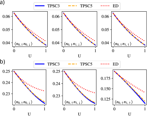
Figure 6: Comparison between TPSC and ED at $\beta=2$, for different $U$ at $J=0$ at quarter filling (panel a) and with an inter-orbital coupling of unit strength (panel b). For these comparisons we include the zeroth order self-energy correction.

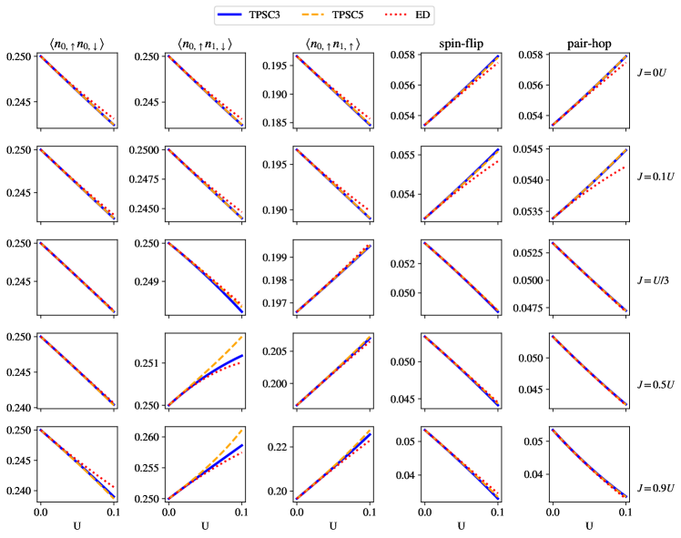
Figure 7: Comparison between TPSC and ED at $\beta=2$, for different $U$ and $J$ combinations. For these comparisons we include the zeroth order self-energy correction.

References

- [1] H. Bethe, Zur theorie der metalle: I. eigenwerte und eigenfunktionen der linearen atomkette, Zeitschrift f”ur Physik 71(3–4), 205–226 (1931), 10.1007/bf01341708.
- [2] J. Luttinger, An exactly soluble model of a many-fermion system, Journal of mathematical physics 4(9), 1154 (1963).
- [3] P. Hohenberg and W. Kohn, Inhomogeneous electron gas, Phys. Rev. 136, B864 (1964), 10.1103/PhysRev.136.B864.
- [4] W. Kohn and L. J. Sham, Self-consistent equations including exchange and correlation effects, Phys. Rev. 140, A1133 (1965), 10.1103/PhysRev.140.A1133.
- [5] A. W. Sandvik and J. Kurkijärvi, Quantum monte carlo simulation method for spin systems, Phys. Rev. B 43, 5950 (1991), 10.1103/PhysRevB.43.5950.
- [6] W. M. C. Foulkes, L. Mitas, R. J. Needs and G. Rajagopal, Quantum monte carlo simulations of solids, Rev. Mod. Phys. 73, 33 (2001), 10.1103/RevModPhys.73.33.
- [7] S. Zhang and H. Krakauer, Quantum monte carlo method using phase-free random walks with slater determinants, Phys. Rev. Lett. 90, 136401 (2003), 10.1103/PhysRevLett.90.136401.
- [8] K. Van Houcke, E. Kozik, N. Prokof’ev and B. Svistunov, Diagrammatic monte carlo, Physics Procedia 6, 95–105 (2010), 10.1016/j.phpro.2010.09.034.
- [9] J. Gubernatis, N. Kawashima and P. Werner, Quantum Monte Carlo methods – Algorithms for lattice models, Cambridge University Press (2016).
- [10] F. Becca and S. Sorella, Quantum Monte Carlo approaches for correlated systems, Cambridge University Press (2017).
- [11] S. R. White, Density matrix formulation for quantum renormalization groups, Phys. Rev. Lett. 69, 2863 (1992), 10.1103/PhysRevLett.69.2863.
- [12] U. Schollwöck, The density-matrix renormalization group in the age of matrix product states, Annals of Physics 326(1), 96–192 (2011), 10.1016/j.aop.2010.09.012.
- [13] J. I. Cirac, D. Pérez-García, N. Schuch and F. Verstraete, Matrix product states and projected entangled pair states: Concepts, symmetries, theorems, Rev. Mod. Phys. 93, 045003 (2021), 10.1103/RevModPhys.93.045003.
- [14] G. Rohringer, H. Hafermann, A. Toschi, A. A. Katanin, A. E. Antipov, M. I. Katsnelson, A. I. Lichtenstein, A. N. Rubtsov and K. Held, Diagrammatic routes to nonlocal correlations beyond dynamical mean field theory, Rev. Mod. Phys. 90, 025003 (2018), 10.1103/RevModPhys.90.025003.
- [15] W. Metzner and D. Vollhardt, Correlated lattice fermions in dimensions, Phys. Rev. Lett. 62, 324 (1989), 10.1103/PhysRevLett.62.324.
- [16] A. Georges, G. Kotliar, W. Krauth and M. J. Rozenberg, Dynamical mean-field theory of strongly correlated fermion systems and the limit of infinite dimensions, Rev. Mod. Phys. 68, 13 (1996), 10.1103/RevModPhys.68.13.
- [17] A. Toschi, A. A. Katanin and K. Held, Dynamical vertex approximation: A step beyond dynamical mean-field theory, Phys. Rev. B 75, 045118 (2007), 10.1103/PhysRevB.75.045118.
- [18] T. Ayral and O. Parcollet, Mott physics and spin fluctuations: A unified framework, Phys. Rev. B 92, 115109 (2015), 10.1103/PhysRevB.92.115109.
- [19] M. Vandelli, J. Kaufmann, M. El-Nabulsi, V. Harkov, A. Lichtenstein and E. Stepanov, Multi-band d-trilex approach to materials with strong electronic correlations, SciPost Physics 13(2) (2022), 10.21468/scipostphys.13.2.036.
- [20] C. Gros, Physics of projected wavefunctions, Annals of Physics 189(1), 53 (1989).
- [21] M. C. Gutzwiller, Correlation of electrons in a narrow band, Phys. Rev. 137, A1726 (1965), 10.1103/PhysRev.137.A1726.
- [22] N. Lanatà, T.-H. Lee, Y.-X. Yao and V. Dobrosavljević, Emergent bloch excitations in mott matter, Phys. Rev. B 96, 195126 (2017), 10.1103/PhysRevB.96.195126.
- [23] D. Guerci, M. Capone and M. Fabrizio, Exciton mott transition revisited, Phys. Rev. Mater. 3, 054605 (2019), 10.1103/PhysRevMaterials.3.054605.
- [24] D. Luo and B. K. Clark, Backflow transformations via neural networks for quantum many-body wave functions, Physical Review Letters 122(22) (2019), 10.1103/physrevlett.122.226401.
- [25] J. Robledo Moreno, G. Carleo, A. Georges and J. Stokes, Fermionic wave functions from neural-network constrained hidden states, Proceedings of the National Academy of Sciences 119(32) (2022), 10.1073/pnas.2122059119.
- [26] N. E. Bickers and S. R. White, Conserving approximations for strongly fluctuating electron systems. ii. numerical results and parquet extension, Phys. Rev. B 43, 8044 (1991), 10.1103/PhysRevB.43.8044.
- [27] G. Esirgen and N. E. Bickers, Fluctuation-exchange theory for general lattice hamiltonians, Phys. Rev. B 55, 2122 (1997), 10.1103/PhysRevB.55.2122.
- [28] W. Metzner, M. Salmhofer, C. Honerkamp, V. Meden and K. Schönhammer, Functional renormalization group approach to correlated fermion systems, Rev. Mod. Phys. 84, 299 (2012), 10.1103/RevModPhys.84.299.
- [29] L. Hedin, New method for calculating the one-particle green’s function with application to the electron-gas problem, Phys. Rev. 139, A796 (1965), 10.1103/PhysRev.139.A796.
- [30] C. Gros and R. Valenti, Cluster expansion for the self-energy: A simple many-body method for interpreting the photoemission spectra of correlated fermi systems, Physical Review B 48(1), 418 (1993).
- [31] D. Sénéchal, D. Perez and M. Pioro-Ladriere, Spectral weight of the hubbard model through cluster perturbation theory, Physical review letters 84(3), 522 (2000).
- [32] N. F. Mott, The basis of the electron theory of metals, with special reference to the transition metals, Proc. Phys. Soc. A 62(7), 416 (1949), 10.1088/0370-1298/62/7/303.
- [33] M. Imada, A. Fujimori and Y. Tokura, Metal-insulator transitions, Rev. Mod. Phys. 70, 1039 (1998), 10.1103/RevModPhys.70.1039.
- [34] C. S. Hellberg and S. C. Erwin, Strongly correlated electrons on a silicon surface: Theory of a mott insulator, Physical Review Letters 83(5), 1003 (1999), 10.1103/physrevlett.83.1003.
- [35] W. F. Brinkman and T. M. Rice, Application of gutzwiller’s variational method to the metal-insulator transition, Phys. Rev. B 2, 4302 (1970), 10.1103/PhysRevB.2.4302.
- [36] G. Esirgen and N. E. Bickers, Fluctuation exchange analysis of superconductivity in the standard three-band model, Phys. Rev. B 57, 5376 (1998), 10.1103/PhysRevB.57.5376.
- [37] C. Honerkamp and M. Salmhofer, Temperature-flow renormalization group and the competition between superconductivity and ferromagnetism, Physical Review B 64(18) (2001), 10.1103/physrevb.64.184516.
- [38] P. W. Anderson, Twenty-five years of high-temperature superconductivity – a personal review, J. Phys.: Conf. Ser. 449, 012001 (2013), 10.1088/1742-6596/449/1/012001.
- [39] V. Crépel and L. Fu, New mechanism and exact theory of superconductivity from strong repulsive interaction, Science Advances 7(30), eabh2233 (2021), 10.1126/sciadv.abh2233.
- [40] B. Edegger, V. N. Muthukumar and C. Gros, Gutzwiller–rvb theory of high-temperature superconductivity: Results from renormalized mean-field theory and variational monte carlo calculations, Advances in Physics 56(6), 927 (2007).
- [41] F. Krien, P. Worm, P. Chalupa-Gantner, A. Toschi and K. Held, Explaining the pseudogap through damping and antidamping on the fermi surface by imaginary spin scattering, Communications Physics 5(1) (2022), 10.1038/s42005-022-01117-5.
- [42] W. Wu, M. Ferrero, A. Georges and E. Kozik, Controlling feynman diagrammatic expansions: Physical nature of the pseudogap in the two-dimensional hubbard model, Phys. Rev. B 96, 041105 (2017), 10.1103/PhysRevB.96.041105.
- [43] M. L. Néel, Propriétés magnétiques des ferrites, ferrimagnétisme et antiferromagnétisme, Ann. Phys. 12(3), 137 (1948), 10.1051/anphys/194812030137.
- [44] L. Savary and L. Balents, Quantum spin liquids: a review, Reports on Progress in Physics 80(1), 016502 (2016), 10.1088/0034-4885/80/1/016502.
- [45] C. Broholm, R. J. Cava, S. A. Kivelson, D. G. Nocera, M. R. Norman and T. Senthil, Quantum spin liquids, Science 367(6475) (2020), 10.1126/science.aay0668.
- [46] R. Kaneko, L. F. Tocchio, R. Valentí and F. Becca, Charge orders in organic charge-transfer salts, New journal of physics 19(10), 103033 (2017).
- [47] C.-W. Chen, J. Choe and E. Morosan, Charge density waves in strongly correlated electron systems, Rep. Prog. Phys. 79(8), 084505 (2016), 10.1088/0034-4885/79/8/084505.
- [48] D. Subires, A. Korshunov, A. H. Said, L. Sánchez, B. R. Ortiz, S. D. Wilson, A. Bosak and S. Blanco-Canosa, Order-disorder charge density wave instability in the kagome metal , Nat Commun 14(1) (2023), 10.1038/s41467-023-36668-w.
- [49] M. Qin, C.-M. Chung, H. Shi, E. Vitali, C. Hubig, U. Schollwöck, S. R. White and S. Zhang, Absence of superconductivity in the pure two-dimensional hubbard model, Phys. Rev. X 10, 031016 (2020), 10.1103/PhysRevX.10.031016.
- [50] T. Schäfer, N. Wentzell, F. Šimkovic, Y.-Y. He, C. Hille, M. Klett, C. J. Eckhardt, B. Arzhang, V. Harkov, F. m. c.-M. Le Régent, A. Kirsch, Y. Wang et al., Tracking the footprints of spin fluctuations: A multimethod, multimessenger study of the two-dimensional hubbard model, Phys. Rev. X 11, 011058 (2021), 10.1103/PhysRevX.11.011058.
- [51] M. Qin, T. Schäfer, S. Andergassen, P. Corboz and E. Gull, The hubbard model: A computational perspective, Annual Review of Condensed Matter Physics 13(1), 275–302 (2022), 10.1146/annurev-conmatphys-090921-033948.
- [52] P. Werner, E. Gull, M. Troyer and A. J. Millis, Spin freezing transition and non-fermi-liquid self-energy in a three-orbital model, Phys. Rev. Lett. 101, 166405 (2008), 10.1103/PhysRevLett.101.166405.
- [53] K. Haule and G. Kotliar, Coherence–incoherence crossover in the normal state of iron oxypnictides and importance of hund’s rule coupling, New journal of physics 11(2), 025021 (2009).
- [54] Z. P. Yin, K. Haule and G. Kotliar, Kinetic frustration and the nature of the magnetic and paramagnetic states in iron pnictides and iron chalcogenides, Nature Materials 10(12), 932–935 (2011), 10.1038/nmat3120.
- [55] A. Georges, L. d. Medici and J. Mravlje, Strong correlations from hund’s coupling, Annual Review of Condensed Matter Physics 4(1), 137–178 (2013), 10.1146/annurev-conmatphys-020911-125045.
- [56] L. de’ Medici, Hund’s induced fermi-liquid instabilities and enhanced quasiparticle interactions, Phys. Rev. Lett. 118, 167003 (2017), 10.1103/PhysRevLett.118.167003.
- [57] H. Ishida and A. Liebsch, Fermi-liquid, non-fermi-liquid, and mott phases in iron pnictides and cuprates, Phys. Rev. B 81, 054513 (2010), 10.1103/PhysRevB.81.054513.
- [58] J. Paglione and R. L. Greene, High-temperature superconductivity in iron-based materials, Nature physics 6(9), 645 (2010).
- [59] H. Hosono, A. Yamamoto, H. Hiramatsu and Y. Ma, Recent advances in iron-based superconductors toward applications, Materials today 21(3), 278 (2018).
- [60] S. Backes, H. O. Jeschke and R. Valentí, Microscopic nature of correlations in multiorbital (): Hund’s coupling versus coulomb repulsion, Phys. Rev. B 92, 195128 (2015), 10.1103/PhysRevB.92.195128.
- [61] J. Mravlje, M. Aichhorn, T. Miyake, K. Haule, G. Kotliar and A. Georges, Coherence-incoherence crossover and the mass-renormalization puzzles in , Phys. Rev. Lett. 106, 096401 (2011), 10.1103/PhysRevLett.106.096401.
- [62] Y. Maeno, S. Yonezawa and A. Ramires, Still mystery after all these years – unconventional superconductivity of – (2024), 2402.12117.
- [63] H. Wadati, J. Mravlje, K. Yoshimatsu, H. Kumigashira, M. Oshima, T. Sugiyama, E. Ikenaga, A. Fujimori, A. Georges, A. Radetinac, K. S. Takahashi, M. Kawasaki et al., Photoemission and dmft study of electronic correlations in : Effects of hund’s rule coupling and possible plasmonic sideband, Phys. Rev. B 90, 205131 (2014), 10.1103/PhysRevB.90.205131.
- [64] M. Wallerberger, A. Hausoel, P. Gunacker, A. Kowalski, N. Parragh, F. Goth, K. Held and G. Sangiovanni, w2dynamics: Local one- and two-particle quantities from dynamical mean field theory, Computer Physics Communications 235, 388 (2019), https://doi.org/10.1016/j.cpc.2018.09.007.
- [65] J. Fink, J. Nayak, E. D. L. Rienks, J. Bannies, S. Wurmehl, S. Aswartham, I. Morozov, R. Kappenberger, M. A. ElGhazali, L. Craco, H. Rosner, C. Felser et al., Evidence of hot and cold spots on the fermi surface of LiFeAs, Phys. Rev. B 99, 245156 (2019), 10.1103/PhysRevB.99.245156.
- [66] K. Zantout, S. Backes and R. Valentí, Effect of nonlocal correlations on the electronic structure of LiFeAs, Physical Review Letters 123(25) (2019), 10.1103/physrevlett.123.256401.
- [67] S. Bhattacharyya, K. Björnson, K. Zantout, D. Steffensen, L. Fanfarillo, A. Kreisel, R. Valentí, B. M. Andersen and P. J. Hirschfeld, Nonlocal correlations in iron pnictides and chalcogenides, Physical Review B 102(3) (2020), 10.1103/physrevb.102.035109.
- [68] G. Kotliar, S. Y. Savrasov, G. Pálsson and G. Biroli, Cellular dynamical mean field approach to strongly correlated systems, Phys. Rev. Lett. 87, 186401 (2001), 10.1103/PhysRevLett.87.186401.
- [69] H. Park, K. Haule and G. Kotliar, Cluster dynamical mean field theory of the mott transition, Phys. Rev. Lett. 101, 186403 (2008), 10.1103/PhysRevLett.101.186403.
- [70] A. I. Lichtenstein and M. I. Katsnelson, Antiferromagnetism and d-wave superconductivity in cuprates: A cluster dynamical mean-field theory, Phys. Rev. B 62, R9283 (2000), 10.1103/PhysRevB.62.R9283.
- [71] M. H. Hettler, A. N. Tahvildar-Zadeh, M. Jarrell, T. Pruschke and H. R. Krishnamurthy, Nonlocal dynamical correlations of strongly interacting electron systems, Phys. Rev. B 58, R7475 (1998), 10.1103/PhysRevB.58.R7475.
- [72] M. H. Hettler, M. Mukherjee, M. Jarrell and H. R. Krishnamurthy, Dynamical cluster approximation: Nonlocal dynamics of correlated electron systems, Phys. Rev. B 61, 12739 (2000), 10.1103/PhysRevB.61.12739.
- [73] E. A. Stepanov, V. Harkov and A. I. Lichtenstein, Consistent partial bosonization of the extended hubbard model, Phys. Rev. B 100, 205115 (2019), 10.1103/PhysRevB.100.205115.
- [74] V. Harkov, M. Vandelli, S. Brener, A. I. Lichtenstein and E. A. Stepanov, Impact of partially bosonized collective fluctuations on electronic degrees of freedom, Phys. Rev. B 103, 245123 (2021), 10.1103/PhysRevB.103.245123.
- [75] J. Kaufmann, C. Eckhardt, M. Pickem, M. Kitatani, A. Kauch and K. Held, Self-consistent ladder dynamical vertex approximation, Physical Review B 103(3) (2021), 10.1103/physrevb.103.035120.
- [76] C. Taranto, S. Andergassen, J. Bauer, K. Held, A. Katanin, W. Metzner, G. Rohringer and A. Toschi, From infinite to two dimensions through the functional renormalization group, Phys. Rev. Lett. 112, 196402 (2014), 10.1103/PhysRevLett.112.196402.
- [77] T. Ayral and O. Parcollet, Mott physics and collective modes: An atomic approximation of the four-particle irreducible functional, Phys. Rev. B 94, 075159 (2016), 10.1103/PhysRevB.94.075159.
- [78] A. Rubtsov, M. Katsnelson and A. Lichtenstein, Dual boson approach to collective excitations in correlated fermionic systems, Annals of Physics 327(5), 1320 (2012), https://doi.org/10.1016/j.aop.2012.01.002.
- [79] J. Kuneš, Efficient treatment of two-particle vertices in dynamical mean-field theory, Phys. Rev. B 83, 085102 (2011), 10.1103/PhysRevB.83.085102.
- [80] Y. M. Vilk and A.-M. Tremblay, Non-perturbative many-body approach to the hubbard model and single-particle pseudogap, Journal de Physique I 7(11), 1309–1368 (1997), 10.1051/jp1:1997135.
- [81] A.-M. S. Tremblay, B. Kyung and D. Sénéchal, Pseudogap and high-temperature superconductivity from weak to strong coupling. towards a quantitative theory (review article), Low Temperature Physics 32(4), 424–451 (2006), 10.1063/1.2199446.
- [82] A.-M. S. Tremblay, Two-Particle-Self-Consistent Approach for the Hubbard Model, p. 409–453, Springer Berlin Heidelberg, ISBN 9783642218316, 10.1007/978-3-642-21831-6_13 (2011).
- [83] Y. M. Vilk, L. Chen and A.-M. S. Tremblay, Theory of spin and charge fluctuations in the hubbard model, Phys. Rev. B 49, 13267 (1994), 10.1103/PhysRevB.49.13267.
- [84] Y. Vilk, L. Chen and A.-M. Tremblay, Two-particle self-consistent theory for spin and charge fluctuations in the hubbard model, Physica C: Superconductivity 235–240, 2235–2236 (1994), 10.1016/0921-4534(94)92339-6.
- [85] S. Arya, P. V. Sriluckshmy, S. R. Hassan and A.-M. S. Tremblay, Antiferromagnetism in the hubbard model on the honeycomb lattice: A two-particle self-consistent study, Physical Review B 92(4) (2015), 10.1103/physrevb.92.045111.
- [86] K. Zantout, M. Altmeyer, S. Backes and R. Valentí, Superconductivity in correlated bedt-ttf molecular conductors: Critical temperatures and gap symmetries, Physical Review B 97(1) (2018), 10.1103/physrevb.97.014530.
- [87] D. Lessnich, C. Gauvin-Ndiaye, R. Valentí and A.-M. S. Tremblay, Spin hall conductivity in the kane-mele-hubbard model at finite temperature, Phys. Rev. B 109, 075143 (2024), 10.1103/PhysRevB.109.075143.
- [88] L. D. Re, Two-particle self-consistent approach for broken symmetry phases (2024), 2312.16280.
- [89] H. Miyahara, R. Arita and H. Ikeda, Development of a two-particle self-consistent method for multiorbital systems and its application to unconventional superconductors, Phys. Rev. B 87, 045113 (2013), 10.1103/PhysRevB.87.045113.
- [90] K. Zantout, S. Backes and R. Valentí, Two‐particle self‐consistent method for the multi‐orbital hubbard model, Annalen der Physik 533(2) (2021), 10.1002/andp.202000399.
- [91] C. Gauvin-Ndiaye, J. Leblanc, S. Marin, N. Martin, D. Lessnich and A.-M. S. Tremblay, Two-particle self-consistent approach for multiorbital models: Application to the emery model, Phys. Rev. B 109, 165111 (2024), 10.1103/PhysRevB.109.165111.
- [92] O. Simard and P. Werner, Nonequilibrium two-particle self-consistent approach, Phys. Rev. B 106, L241110 (2022), 10.1103/PhysRevB.106.L241110.
- [93] J. Yan and P. Werner, Spin correlations in the bilayer hubbard model with perpendicular electric field (2023), 2312.15776.
- [94] N. Martin, C. Gauvin-Ndiaye and A.-M. S. Tremblay, Nonlocal corrections to dynamical mean-field theory from the two-particle self-consistent method, Phys. Rev. B 107, 075158 (2023), 10.1103/PhysRevB.107.075158.
- [95] K. Zantout, S. Backes, A. Razpopov, D. Lessnich and R. Valentí, Improved effective vertices in the multiorbital two-particle self-consistent method from dynamical mean-field theory, Physical Review B 107(23) (2023), 10.1103/physrevb.107.235101.
- [96] O. Simard and P. Werner, Dynamical mean field theory extension to the nonequilibrium two-particle self-consistent approach, Physical Review B 107(24) (2023), 10.1103/physrevb.107.245137.
- [97] J. Otsuki, Two-particle self-consistent approach to unconventional superconductivity, Phys. Rev. B 85, 104513 (2012), 10.1103/PhysRevB.85.104513.
- [98] Y. M. Vilk and A.-M. S. Tremblay, Destruction of fermi-liquid quasiparticles in two dimensions by critical fluctuations, Europhysics Letters (EPL) 33(2), 159–164 (1996), 10.1209/epl/i1996-00315-2.
- [99] S. Allen, A. M. S. Tremblay and Y. M. Vilk, Conserving approximations vs two-particle self-consistent approach (2003), cond-mat/0110130.
- [100] S. Allen and A.-M. S. Tremblay, Nonperturbative approach to the attractive hubbard model, Phys. Rev. B 64, 075115 (2001), 10.1103/PhysRevB.64.075115.
- [101] B. Kyung, J.-S. Landry and A.-M. S. Tremblay, Antiferromagnetic fluctuations and d-wave superconductivity in electron-doped high-temperature superconductors, Phys. Rev. B 68, 174502 (2003), 10.1103/PhysRevB.68.174502.
- [102] S. R. Hassan, B. Davoudi, B. Kyung and A.-M. S. Tremblay, Conditions for magnetically induced singlet -wave superconductivity on the square lattice, Phys. Rev. B 77, 094501 (2008), 10.1103/PhysRevB.77.094501.
- [103] C. Gauvin-Ndiaye, P.-A. Graham and A.-M. S. Tremblay, Disorder effects on hot spots in electron-doped cuprates, Phys. Rev. B 105, 235133 (2022), 10.1103/PhysRevB.105.235133.
- [104] C. Gauvin-Ndiaye, C. Lahaie, Y. M. Vilk and A.-M. S. Tremblay, Improved two-particle self-consistent approach for the single-band hubbard model in two dimensions, Phys. Rev. B 108, 075144 (2023), 10.1103/PhysRevB.108.075144.
- [105] M. Salmhofer and C. Honerkamp, Fermionic renormalization group flows: Technique and theory, Progress of Theoretical Physics 105(1), 1–35 (2001), 10.1143/ptp.105.1.
- [106] C. Honerkamp, Efficient vertex parametrization for the constrained functional renormalization group for effective low-energy interactions in multiband systems, Phys. Rev. B 98, 155132 (2018), 10.1103/PhysRevB.98.155132.
- [107] D. Lessnich, C. Gauvin-Ndiaye, R. Valentí and A.-M. S. Tremblay, Spin hall conductivity in the kane-mele-hubbard model at finite temperature, Phys. Rev. B 109, 075143 (2024), 10.1103/PhysRevB.109.075143.
- [108] Pyed: Exact diagonalization for finite quantum systems, https://github.com/HugoStrand/pyed, Accessed: 2024-07-15.
- [109] O. Parcollet, M. Ferrero, T. Ayral, H. Hafermann, I. Krivenko, L. Messio and P. Seth, TRIQS: A toolbox for research on interacting quantum systems, Computer Physics Communications 196, 398 (2015), 10.1016/j.cpc.2015.04.023, 1504.01952.
- [110] A. L. Fetter and J. D. Walecka, Quantum theory of many-particle systems, Courier Corporation (2012).