Simulating binary black hole mergers using discontinuous Galerkin methods

Abstract

Binary black holes are the most abundant source of gravitational-wave observations. Gravitational-wave observatories in the next decade will require tremendous increases in the accuracy of numerical waveforms modeling binary black holes, compared to today’s state of the art. One approach to achieving the required accuracy is using spectral-type methods that scale to many processors. Using the SpECTRE numerical-relativity code, we present the first simulations of a binary black hole inspiral, merger, and ringdown using discontinuous Galerkin methods. The efficiency of discontinuous Galerkin methods allows us to evolve the binary through $\sim 18$ orbits at reasonable computational cost. We then use SpECTRE’s Cauchy Characteristic Evolution (CCE) code to extract the gravitational waves at future null infinity. The open-source nature of SpECTRE means this is the first time a spectral-type method for simulating binary black hole evolutions is available to the entire numerical-relativity community.

Keywords: discontinuous Galerkin, binary black holes, numerical relativity

1 Introduction

Binary black holes are the most abundant source of gravitational-wave observations to date [1]. Realizing the scientific potential of these observations requires accurate models of the emitted gravitational waves as the black holes inspiral, merge, and ring down to a final, stationary state. Building these models requires numerical-relativity (NR) simulations of binary black holes, because analytic approximations (e.g. the post-Newtonian [2] approximation) alone break down near the time of merger.

Since the first breakthrough simulations [3, 4, 5], the NR community has developed codes capable of evolving two black holes through inspiral, merger, and ringdown (see [6, 7] for a review). Several groups have used NR codes to build catalogs of gravitational waveforms for applications to gravitational-wave astronomy [8, 9, 10, 11, 12, 13, 14, 15]. Today’s NR codes are sufficiently accurate for the observations that LIGO and Virgo are making. However, observatories planned for the next decade, including the Einstein Telescope [16] and Cosmic Explorer [17] on Earth and the Laser Interferometer Space Antenna (LISA) [18] in space, will be so sensitive that they will require NR waveforms with a substantial increase in accuracy [19, 20, 21].

Spectral-type methods are extremely efficient; this makes them a promising avenue toward the ultimate goal of achieving the needed accuracy for future gravitational-wave observatories. In comparison, almost all current NR codes for evolving binary black holes use finite-difference methods, with numerical errors decreasing as a power law with increasing resolution. However, recent results from the AthenaK code [22] show that finite-difference methods using graphics processing units (GPUs) might be another approach to achieving the required accuracy. The Spectral Einstein Code (SpEC) [23] uses a pseudospectral method (see [24] for a review of these methods) to construct and evolve binary-black-hole initial data. With pseudospectral methods, errors decrease exponentially with increasing number of grids points in the computational domain’s elements (“$p$-refinement”). SpEC’s exponential convergence makes it highly efficient, but its performance, and therefore the achievable accuracy, is limited by aspects of its design. For instance, because it uses computational domains divided into a small number of high-resolution elements, SpEC simulations of binary black holes cannot scale beyond $\mathcal{O}(10^{2})$ CPU cores. SpEC is also a closed-source code, unavailable to most of the NR community. Other examples of pseudospectral or spectral methods being used for solving the initial value problem are Elliptica [25], FUKA [26], and bamps [27]. In terms of evolving spacetimes, the Nmesh [28] code has been used to successfully simulate single black holes using discontinuous Galerkin methods, and the bamps [29, 30] code uses pseudospectral methods to evolve spacetimes with single dynamical black holes with a focus on critical behavior [31, 32, 33, 34, 35, 36, 37, 38] but has also simulated boson stars [39]. Recently, [40] performed a 0.5 orbit grazing collision of two black holes (a similar setup to [41]) using a finite volume grid in the strong field region and a DG method in the wave zone.

We present the first simulations of a binary black hole inspiral, merger, and ringdown using a discontinuous Galerkin (DG) method [42] (see [43] for a review of DG). The efficiency of DG methods allows us to evolve the binary through $\sim 18$ orbits at reasonable computational cost. DG, being a spectral-type method, has exponential convergence with $p$-refinement. In this work, we present SpECTRE’s [44] first simulations of $\sim 18$ orbits of inspiral, merger, and ringdown of an equal-mass, non-spinning binary black hole, using DG methods. We then use SpECTRE’s Cauchy Characteristic Evolution module [45, 46, 44] to evolve the gravitational waves to future null infinity. These results demonstrate that DG methods can provide high-accuracy gravitational waveforms from binary black hole mergers for application to gravitational-wave data analysis. By implementing our approach in SpECTRE, an open-source NR code, we are also making a spectral-type binary-black-hole evolution code available to the entire NR community for the first time.

The rest of this paper is organized as follows. In §2, we discuss the numerical methods used in SpECTRE’s binary-black-hole simulations. Then, in §3, we first test our method’s stability with simulations of single black holes before presenting results for simulations of binary black holes with SpECTRE. We briefly conclude in §4.

2 Methods

2.1 Equations of Motion

We adopt the standard 3+1 form of the spacetime metric, (see, e.g., [47, 48]),

$$ds^{2} =g_{ab}dx^{a}dx^{b}=-\alpha^{2}dt^{2}+\gamma_{ij}\left(dx^{i}+\beta^{i}dt\right)\left(dx^{j}+\beta^{j}dt\right),$$ (1)

where $\alpha$ is the lapse, $\beta^{i}$ the shift vector, and $\gamma_{ij}$ is the spatial metric. We use the Einstein summation convention, summing over repeated indices. Latin indices from the first part of the alphabet $a,b,c,\ldots$ denote spacetime indices ranging from $0$ to $3$, while Latin indices $i,j,\ldots$ are purely spatial, ranging from $1$ to $3$. We work in units where $c=G=1$.

We evolve the first-order generalized harmonic (FOGH) system, given by [49],

$$\partial_{t}g_{ab} =\left(1+\gamma_{1}\right)\beta^{k}\partial_{k}g_{ab}-\alpha\Pi_{ab}-\gamma_{1}\beta^{i}\Phi_{iab}+\gamma_{1}v^{k}_{g}\left(\partial_{k}g_{ab}-\Phi_{kab}\right),$$ (2)

$$\partial_{t}\Phi_{iab} =\beta^{k}\partial_{k}\Phi_{iab}-\alpha\partial_{i}\Pi_{ab}+\alpha\gamma_{2}\partial_{i}g_{ab}+\frac{1}{2}\alpha n^{c}n^{d}\Phi_{icd}\Pi_{ab}$$ (3)

$$+\alpha\gamma^{jk}n^{c}\Phi_{ijc}\Phi_{kab}-\alpha\gamma_{2}\Phi_{iab},$$

$$\partial_{t}\Pi_{ab} =\beta^{k}\partial_{k}\Pi_{ab}-\alpha\gamma^{ki}\partial_{k}\Phi_{iab}+\gamma_{1}\gamma_{2}\beta^{k}\partial_{k}g_{ab}$$ (4)

$$+2\alpha g^{cd}\left(\gamma^{ij}\Phi_{ica}\Phi_{jdb}-\Pi_{ca}\Pi_{db}-g^{ef}\Gamma_{ace}\Gamma_{bdf}\right)$$

$$-2\alpha\nabla_{(a}H_{b)}-\frac{1}{2}\alpha n^{c}n^{d}\Pi_{cd}\Pi_{ab}-\alpha n^{c}\Pi_{ci}\gamma^{ij}\Phi_{jab}$$

$$+\alpha\gamma_{0}\left(2\delta^{c}{}_{(a}n_{b)}-g_{ab}n^{c}\right)\mathcal{C}_{c}-\gamma_{1}\gamma_{2}\beta^{i}\Phi_{iab},$$

where $g_{ab}$ is the spacetime metric, $\Phi_{iab}=\partial_{i}g_{ab}$, $\Pi_{ab}=n^{c}\partial_{c}g_{ab}$, $n^{a}$ is the unit normal vector to the spatial slice, $\gamma_{0}$ damps the 1-index or gauge constraint $\mathcal{C}_{a}=H_{a}+\Gamma_{a}$, $\gamma_{1}$ controls the linear degeneracy of the system, $\gamma_{2}$ damps the 3-index constraint $\mathcal{C}_{iab}=\partial_{i}g_{ab}-\Phi_{iab}$, $\Gamma_{abc}$ are the spacetime Christoffel symbols of the first kind, $\Gamma_{a}=g^{bc}\Gamma_{bca}$, and $v^{k}_{g}$ is the grid/mesh velocity as discussed in §2.2.

The gauge source function $H_{a}$ can be any arbitrary function depending only upon the spacetime coordinates $x^{a}$ and $g_{ab}$, but not derivatives of $g_{ab}$, since that may spoil the strong hyperbolicity of the system [50, 51].

Defining $s_{i}$ to be the unit normal covector to a 2d surface with $s_{a}=(0,s_{i})$, and $s^{a}=g^{ab}s_{b}$, the characteristic fields for the FOGH system are [49]

$$w^{g}_{ab} =g_{ab},$$ (5)

$$w^{0}_{iab} =(\delta^{k}_{i}-s^{k}s_{i})\Phi_{kab},$$ (6)

$$w^{\pm}_{ab} =\Pi_{ab}\pm s^{i}\Phi_{iab}-\gamma_{2}g_{ab},$$ (7)

with associated characteristic speeds

$$\lambda_{w^{g}}= -(1+\gamma_{1})\beta^{i}s_{i}-(1+\gamma_{1})v^{i}_{g}s_{i},$$ (8)

$$\lambda_{w^{0}}= -\beta^{i}s_{i}-v^{i}_{g}s_{i},$$ (9)

$$\lambda_{w^{\pm}}= \pm\alpha-\beta^{i}s_{i}-v^{i}_{g}s_{i},$$ (10)

where we denote the velocity of the grid/mesh as $v^{i}_{g}$ (see §2.2 for details on our moving mesh method). The evolved variables as a function of the characteristic fields are given by

$$g_{ab} =w^{g}_{ab},$$ (11)

$$\Pi_{ab} =\frac{1}{2}\left(w^{+}_{ab}+w^{-}_{ab}\right)+\gamma_{2}w^{g}_{ab},$$ (12)

$$\Phi_{iab} =\frac{1}{2}\left(w^{+}_{ab}-w^{-}_{ab}\right)s_{i}+w^{0}_{iab}.$$ (13)

The constraints for the FOGH system are [49]

$$\mathcal{C}_{a} =H_{a}+\Gamma_{a},$$ (14)

$$\mathcal{C}_{ia} =\gamma^{jk}\partial_{j}\Phi_{ika}-\frac{1}{2}\gamma_{a}^{j}g^{cd}\partial_{j}\Phi_{icd}+n^{b}\partial_{i}\Pi_{ba}-\frac{1}{2}n_{a}g^{cd}\partial_{i}\Pi_{cd}$$ (15)

$$+\partial_{i}H_{a}+\frac{1}{2}\gamma_{a}^{j}\Phi_{jcd}\Phi_{ief}g^{ce}g^{df}+\frac{1}{2}\gamma^{jk}\Phi_{jcd}\Phi_{ike}g^{cd}n^{e}n_{a}$$

$$-\gamma^{jk}\gamma^{mn}\Phi_{jma}\Phi_{ikn}+\frac{1}{2}\Phi_{icd}\Pi_{be}n_{a}\left(g^{cb}g^{de}+\frac{1}{2}g^{be}n^{c}n^{d}\right)$$

$$-\Phi_{icd}\Pi_{ba}n^{c}\left(g^{bd}+\frac{1}{2}n^{b}n^{d}\right)+\frac{1}{2}\gamma_{2}\left(n_{a}g^{cd}-2\delta^{c}_{a}n^{d}\right)\mathcal{C}_{icd},$$

$$\mathcal{C}_{iab} =\partial_{i}g_{ab}-\Phi_{iab},$$ (16)

$$\mathcal{C}_{ijab} =\partial_{i}\Phi_{jab}-\partial_{j}\Phi_{iab},$$ (17)

and

$$\mathcal{F}_{a} =\frac{1}{2}\gamma_{a}^{i}g^{bc}\partial_{i}\Pi_{bc}-\gamma^{ij}\partial_{i}\Pi_{ja}-\gamma^{ij}n^{b}\partial_{i}\Phi_{jba}+\frac{1}{2}n_{a}g^{bc}\gamma^{ij}\partial_{i}\Phi_{jbc}$$ (18)

$$+n_{a}\gamma^{ij}\partial_{i}H_{j}+\gamma_{a}^{i}\Phi_{ijb}\gamma^{jk}\Phi_{kcd}g^{bd}n^{c}-\frac{1}{2}\gamma_{a}^{i}\Phi_{ijb}\gamma^{jk}\Phi_{kcd}g^{cd}n^{b}$$

$$-\gamma_{a}^{i}n^{b}\partial_{i}H_{b}+\gamma^{ij}\Phi_{icd}\Phi_{jba}g^{bc}n^{d}-\frac{1}{2}n_{a}\gamma^{ij}\gamma^{mn}\Phi_{imc}\Phi_{njd}g^{cd}$$

$$-\frac{1}{4}n_{a}\gamma^{ij}\Phi_{icd}\Phi_{jbe}g^{cb}g^{de}+\frac{1}{4}n_{a}\Pi_{cd}\Pi_{be}g^{cb}g^{de}-\gamma^{ij}H_{i}\Pi_{ja}$$

$$-n^{b}\gamma^{ij}\Pi_{bi}\Pi_{ja}-\frac{1}{4}\gamma_{a}^{i}\Phi_{icd}n^{c}n^{d}\Pi_{be}g^{be}+\frac{1}{2}n_{a}\Pi_{cd}\Pi_{be}g^{ce}n^{d}n^{b}$$

$$+\gamma_{a}^{i}\Phi_{icd}\Pi_{be}n^{c}n^{b}g^{de}-\gamma^{ij}\Phi_{iba}n^{b}\Pi_{je}n^{e}-\frac{1}{2}\gamma^{ij}\Phi_{icd}n^{c}n^{d}\Pi_{ja}$$

$$-\gamma^{ij}H_{i}\Phi_{jba}n^{b}+\gamma_{a}^{i}\Phi_{icd}H_{b}g^{bc}n^{d}+\gamma_{2}\left(\gamma^{id}\mathcal{C}_{ida}-\frac{1}{2}\gamma_{a}^{i}g^{cd}\mathcal{C}_{icd}\right)$$

$$+\frac{1}{2}n_{a}\Pi_{cd}g^{cd}H_{b}n^{b}-n_{a}\gamma^{ij}\Phi_{ijc}H_{d}g^{cd}+\frac{1}{2}n_{a}\gamma^{ij}H_{i}\Phi_{jcd}g^{cd}.$$

While only the gauge constraint (14) and 3-index constraint (16) are damped, all constraints can be monitored to check the accuracy of the numerical simulation. All the constraints can be combined into a scalar, the constraint energy, given by [49]

$$\mathcal{E} =\delta^{ab}\left[\mathcal{C}_{a}\mathcal{C}_{b}+\left(\mathcal{F}_{a}\mathcal{F}_{b}+\mathcal{C}_{ia}\mathcal{C}_{jb}\gamma^{ij}\right)\right]$$ (19)

$$+\delta^{ab}\delta^{cd}\left(\mathcal{C}_{iac}\mathcal{C}_{jbd}\gamma^{ij}+\mathcal{C}_{ikac}\mathcal{C}_{jlbd}\gamma^{ij}\gamma^{kl}\right).$$

In practice we have also found that it is typically only necessary to monitor violations of the constraints $\mathcal{C}_{a}$ and $\mathcal{C}_{iab}$, because they typically grow first and the other violations grow as a consequence.

2.2 Discontinuous Galerkin Method

SpECTRE uses a discontinuous Galerkin method for the spatial discretization. We refer readers to [52, 53] and references therein for a detailed discussion of the method and its implementation in SpECTRE; here we summarize the necessary results. The FOGH equations are a first-order strongly hyperbolic system in non-conservative form, which takes the general form

$$\partial_{t}u_{\alpha}+B_{\alpha\beta}^{i}(u_{\alpha})\partial_{i}u_{\beta}=S_{\alpha}(u_{\alpha}),$$ (20)

where $u_{\alpha}=\{g_{ab},\Phi_{iab},\Pi_{ab}\}$ is the state vector of evolved variables, $B_{\alpha\beta}^{i}(u)$ is a matrix that depends only on $u_{\alpha}$, and $S_{\alpha}(u)$ are source terms that also only depend on $u_{\alpha}$. We denote the logical coordinates of our Legendre-Gauss-Lobatto DG scheme by $\{\hat{t},\xi^{\hat{\imath}}\}=\{\hat{t},\xi,\eta,\zeta\}$ and the inertial coordinates as $\{t=\hat{t},x^{i}(\hat{t},\xi^{\hat{\imath}})\}$. We are using a moving mesh as in [54, 52]; therefore, the mapping from logical to inertial coordinates is time dependent. We denote the determinant of the spatial Jacobian of this map as

$$J=\det\left(\frac{\partial x^{i}}{\partial\xi^{\hat{\imath}}}\right),$$ (21)

and the grid or mesh velocity by [54, 52]

$$v_{g}^{i}=\partial_{\hat{t}}x^{i}.$$ (22)

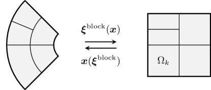
Figure 1: A diagram of the forward and reverse mappings $x^{i}(\hat{t},\xi^{\hat{\imath}})$ and $\xi^{\hat{\imath}}(t,x^{i})$, respectively, from logical (right side of the diagram) to inertial coordinates (left side of the diagram) for an element $\Omega_{k}$.

SpECTRE decomposes the domain into a set of non-overlapping hexahedra which are deformed using the map $x^{i}(\hat{t},\xi^{\hat{\imath}})$ illustrated in figure 1. SpECTRE uses a different number of grid points in each logical direction, which we denote by $N_{\breve{\imath}}$ in the $\xi$ direction, $N_{\breve{\jmath}}$ in the $\eta$ direction, and $N_{\breve{k}}$ in the $\zeta$ direction below.

Since we use a moving mesh, we evolve the system

$$\partial_{\hat{t}}u_{\alpha}+\left[B_{\alpha\beta}^{i}(u_{\alpha})-v^{i}_{g}\delta_{\alpha\beta}\right]\partial_{i}u_{\beta}=S(u_{\alpha}).$$ (23)

We denote grid point and modal indices with a breve, i.e. $u_{\breve{\imath}\breve{\jmath}\breve{k}}$ is the value of $u$ at the grid point $(\breve{\imath},\breve{\jmath},\breve{k})$. The semi-discrete equations are given by [54, 52]

$$(\partial_{\hat{t}}u_{\alpha})_{\breve{\imath}\breve{\jmath}\breve{k}} =(S_{\alpha})_{\breve{\imath}\breve{\jmath}\breve{k}}-\left(B_{\alpha\beta}^{i}-v^{i}_{g}\delta_{\alpha\beta}\right)_{\breve{\imath}\breve{\jmath}\breve{k}}\left[\left(\frac{\partial\xi^{\hat{1}}}{\partial x^{i}}\right)_{\breve{\imath}\breve{\jmath}\breve{k}}\sum_{\breve{l}}D^{(\hat{1})}_{\breve{\imath}\breve{l}}(u_{\beta})_{\breve{l}\breve{\jmath}\breve{k}}\right.$$ (24)

$$-\left.\left(\frac{\partial\xi^{\hat{2}}}{\partial x^{i}}\right)_{\breve{\imath}\breve{\jmath}\breve{k}}\sum_{\breve{l}}D^{(\hat{2})}_{\breve{\jmath}\breve{l}}(u_{\beta})_{\breve{\imath}\breve{l}\breve{k}}+\left(\frac{\partial\xi^{\hat{3}}}{\partial x^{i}}\right)_{\breve{\imath}\breve{\jmath}\breve{k}}\sum_{\breve{l}}D^{(\hat{3})}_{\breve{k}\breve{l}}(u_{\beta})_{\breve{\imath}\breve{\jmath}\breve{l}}\right]$$

$$-\frac{\delta_{N_{\breve{k}}\breve{k}}}{w_{\breve{k}}J_{\breve{\imath}\breve{\jmath}\breve{k}}}\left\{\left[J\sqrt{\frac{\partial\xi^{\hat{3}}}{\partial x^{i}}\gamma^{ij}\frac{\partial\xi^{\hat{3}}}{\partial x^{j}}}D_{\alpha}\right]_{\breve{\imath}\breve{\jmath}N_{\breve{k}}}+\left[J\sqrt{\frac{\partial\xi^{\hat{3}}}{\partial x^{i}}\gamma^{ij}\frac{\partial\xi^{\hat{3}}}{\partial x^{j}}}D_{\alpha}\right]_{\breve{\imath}\breve{\jmath}0}\right\}$$

$$-\frac{\delta_{N_{\breve{\jmath}}\breve{\jmath}}}{w_{\breve{\jmath}}J_{\breve{\imath}\breve{\jmath}\breve{k}}}\left\{\left[J\sqrt{\frac{\partial\xi^{\hat{3}}}{\partial x^{i}}\gamma^{ij}\frac{\partial\xi^{\hat{3}}}{\partial x^{j}}}D_{\alpha}\right]_{\breve{\imath}N_{\breve{\jmath}}\breve{k}}+\left[J\sqrt{\frac{\partial\xi^{\hat{3}}}{\partial x^{i}}\gamma^{ij}\frac{\partial\xi^{\hat{3}}}{\partial x^{j}}}D_{\alpha}\right]_{\breve{\imath}0\breve{k}}\right\}$$

$$-\frac{\delta_{N_{\breve{\imath}}\breve{\imath}}}{w_{\breve{\imath}}J_{\breve{\imath}\breve{\jmath}\breve{k}}}\left\{\left[J\sqrt{\frac{\partial\xi^{\hat{3}}}{\partial x^{i}}\gamma^{ij}\frac{\partial\xi^{\hat{3}}}{\partial x^{j}}}D_{\alpha}\right]_{N_{\breve{\imath}}\breve{\jmath}\breve{k}}+\left[J\sqrt{\frac{\partial\xi^{\hat{3}}}{\partial x^{i}}\gamma^{ij}\frac{\partial\xi^{\hat{3}}}{\partial x^{j}}}D_{\alpha}\right]_{0\breve{\jmath}\breve{k}}\right\},$$

where $w_{\breve{\imath}}$ are the Legendre-Gauss-Lobatto integration weights. We use a method of lines approach to integrate these in time, with the details discussed in §2.5 below.

For the boundary terms $D_{\alpha}$, we use an upwind multi-penalty method [55, 56, 57, 24] given by

$$D_{g_{ab}} =\tilde{\lambda}_{w^{g}}^{\mathrm{ext}}w^{\mathrm{ext},g}_{ab}-\tilde{\lambda}_{w^{g}}^{\mathrm{int}}w^{\mathrm{int},g}_{ab},$$ (25)

$$D_{\Pi_{ab}} =\frac{1}{2}\left(\tilde{\lambda}_{w^{+}}^{\mathrm{ext}}w^{\mathrm{ext},+}_{ab}+\tilde{\lambda}_{w^{-}}^{\mathrm{ext}}w^{\mathrm{ext},-}_{ab}\right)+\tilde{\lambda}_{w^{g}}^{\mathrm{ext}}\gamma_{2}w^{\mathrm{ext},g}_{ab}$$ (26)

$$-\frac{1}{2}\left(\tilde{\lambda}_{w^{+}}^{\mathrm{int}}w^{\mathrm{int},+}_{ab}+\tilde{\lambda}_{w^{-}}^{\mathrm{int}}w^{\mathrm{int},-}_{ab}\right)-\tilde{\lambda}_{w^{g}}^{\mathrm{int}}\gamma_{2}w^{\mathrm{int},g}_{ab},$$

$$D_{\Phi_{iab}} =\frac{1}{2}\left(\tilde{\lambda}_{w^{+}}^{\mathrm{ext}}w^{\mathrm{ext},+}_{ab}-\tilde{\lambda}_{w^{-}}^{\mathrm{ext}}w^{\mathrm{ext},-}_{ab}\right)s_{i}^{\mathrm{ext}}+\tilde{\lambda}_{w^{0}}^{\mathrm{ext}}w^{\mathrm{ext},0}_{iab}$$ (27)

$$-\frac{1}{2}\left(\tilde{\lambda}_{w^{+}}^{\mathrm{int}}w^{\mathrm{int},+}_{ab}-\tilde{\lambda}_{w^{-}}^{\mathrm{int}}w^{\mathrm{int},-}_{ab}\right)s_{i}^{\mathrm{int}}-\tilde{\lambda}_{w^{0}}^{\mathrm{int}}w^{\mathrm{int},0}_{iab},$$

where the spatial normal vector to the element interface $s^{\mathrm{int}}_{i}$ is pointing out of the DG element and $\tilde{\lambda}=0$ if $\lambda>0$, otherwise $\tilde{\lambda}=\lambda$, i.e. $\tilde{\lambda}=\lambda\Theta(-\lambda)$. Note that we assume $s^{\mathrm{ext}}_{i}$ and $s^{\mathrm{int}}_{i}$ point in the same direction. Also note that these boundary flux terms differ from the multi-penalty approach used in SpEC by a factor of $2$. That is,

$$D^{\mathtt{SpECTRE}}=2D^{\mathtt{SpEC}},$$ (28)

ultimately because the lifting terms are different. In SpEC and, similarly in bamps[29], the penalty term is derived from requiring that the total energy be non-increasing, while in SpECTRE the terms come from an integration by parts when deriving the semi-discrete DG equations.

2.3 Boundary conditions

At the outer radial boundary, we apply constraint-preserving boundary conditions [49, 58] by adding terms to the time derivative of the characteristic fields and thus also the time derivatives of the evolved variables. We use the characteristic fields and speeds defined in §2.1. We define $d_{\hat{t}}w_{\hat{\alpha}}$ as the time derivatives substituted into the transformation equations to the characteristic fields. That is,

$$d_{\hat{t}}w^{g}_{ab} =\partial_{\hat{t}}g_{ab},$$ (29)

$$d_{\hat{t}}w^{0}_{iab} =(\delta^{k}_{i}-s^{k}s_{i})\partial_{\hat{t}}\Phi_{kab},$$ (30)

$$d_{\hat{t}}w^{\pm}_{ab} =\partial_{\hat{t}}\Pi_{ab}\pm s^{i}\partial_{\hat{t}}\Phi_{iab}-\gamma_{2}\partial_{\hat{t}}g_{ab}.$$ (31)

We also define $D_{\hat{t}}w_{\hat{\alpha}}$ as the characteristic field transformation of the volume right-hand-side, i.e. $\partial_{\hat{t}}u_{\alpha}$ without any boundary terms. Finally, for brevity we define the projection tensor $P_{ab}=g_{ab}+n_{a}n_{b}-s_{a}s_{b}$, the inward directed null vector field $k^{a}=(n^{a}-s^{a})/\sqrt{2}$, and the outgoing null vector field $l^{a}=(n^{a}+s^{a})/\sqrt{2}$.

The fields $d_{\hat{t}}w^{g}_{ab}$ and $d_{\hat{t}}w^{0}_{iab}$ are determined solely by the constraint-preserving boundary condition, while the boundary condition for $d_{\hat{t}}w^{-}_{ab}$ is composed of three parts: the constraint preserving part, the physical part, and the gauge part. We denote these as $B_{ab}^{C}$, $B_{ab}^{P}$ and $B_{ab}^{G}$. With this, the boundary conditions imposed on the fields are

$$d_{\hat{t}}w^{g}_{ab} =D_{\hat{t}}w^{g}_{ab}+\lambda_{w^{g}}s^{i}\mathcal{C}_{iab},$$ (32)

$$d_{\hat{t}}w^{0}_{kab} =D_{\hat{t}}w^{0}_{ab}+\lambda_{w^{0}}s^{i}P^{j}{}_{k}\mathcal{C}_{ijab},$$ (33)

$$d_{\hat{t}}w^{-}_{ab} =D_{\hat{t}}w^{-}_{ab}+\lambda_{w^{-}}\left[B_{ab}^{C}+B_{ab}^{P}+B_{ab}^{G}\right].$$ (34)

Transforming to the evolved variables we find that the following terms need to be added in order to impose the boundary condition,

$$\partial_{\hat{t}}g_{ab} \to\partial_{\hat{t}}g_{ab}+\lambda_{w^{g}}s^{i}\mathcal{C}_{iab},$$ (35)

$$\partial_{\hat{t}}\Pi_{ab} \to\partial_{\hat{t}}\Pi_{ab}+\frac{1}{2}\lambda_{w^{-}}\left[B_{ab}^{C}+B_{ab}^{P}+B_{ab}^{G}\right]+\gamma_{2}\lambda_{w^{g}}s^{i}\mathcal{C}_{iab},$$ (36)

$$\partial_{\hat{t}}\Phi_{iab} \to\partial_{\hat{t}}\Phi_{iab}-\frac{s_{i}}{2}\lambda_{w^{-}}\left[B_{ab}^{C}+B_{ab}^{P}+B_{ab}^{G}\right]+\lambda_{w^{0}}s^{i}P^{j}{}_{k}\mathcal{C}_{ijab}.$$ (37)

We now need to specify the $B_{ab}$ boundary conditions. The constraint-preserving part is

$$B_{ab}^{C}=\sqrt{2}\left(\frac{1}{2}P_{ab}l^{c}+\frac{1}{2}l_{a}l_{b}k^{c}-l_{(a}P_{b)}{}^{c}\right)\left(\mathcal{F}_{c}-s^{k}\mathcal{C}_{kc}\right).$$ (38)

The physical boundary conditions are determined by the propagating parts of the Weyl curvature tensor. That is,

$$B_{ab}^{P}=\left(P_{a}{}^{c}P_{b}{}^{d}-\frac{1}{2}P_{ab}P^{cd}\right)\left[C^{-}_{cd}-\gamma_{2}s^{i}\mathcal{C}_{icd}\right],$$ (39)

where $C^{-}_{ab}$ is the inward propagating part of the Weyl tensor, given by

$$C^{\pm}_{ab}=\left(P_{a}{}^{c}P_{b}{}^{d}-\frac{1}{2}P_{ab}P^{cd}\right)\left(n^{e}\mp s^{e}\right)\left(n^{f}\mp s^{f}\right)C_{cedf}.$$ (40)

For the simulations presented here, we set $C^{-}_{ab}=0$, though Cauchy-Characteristic matching [59] can be used to prescribe a more physically motivated boundary condition. Recently [60] presented an alternative approach to Cauchy-Characteristic matching for providing high-order non-reflecting boundary conditions. Finally, the gauge boundary condition is set using a Sommerfeld condition on the components not set by the constraint-preserving and physical boundary conditions. The projector for the gauge boundary condition is given by

$$\delta_{a}^{c}\delta_{b}^{d}-P^{C}_{ab}{}^{cd}-P^{P}_{ab}{}^{cd} =\delta_{a}^{c}\delta_{b}^{d}-\frac{1}{2}P_{ab}P^{cd}+2\l_{(a}P_{b)}{}^{(c}k^{d)}$$ (41)

$$-l_{a}l_{b}k^{c}k^{d}-P_{a}{}^{c}P_{b}{}^{d}+\frac{1}{2}P_{ab}P^{cd}$$

$$=\delta_{a}^{c}\delta_{b}^{d}+2\l_{(a}P_{b)}{}^{(c}k^{d)}-l_{a}l_{b}k^{c}k^{d}-P_{a}{}^{c}P_{b}{}^{d}.$$

The Sommerfeld condition is

$$B_{ab}^{G}=\frac{1}{\lambda_{w^{-}}}\left(2\l_{(a}P_{b)}{}^{(c}k^{d)}-2k_{(a}l_{b)}k^{(c}l^{d)}-k_{a}k_{b}l^{c}l^{d}\right)\left(\gamma_{2}-\frac{1}{r}\right)\partial_{t}g_{cd}.$$ (42)

When evolving spacetimes with black holes, we excise the interior of the black hole as is done in SpEC [49]. At excision boundaries, all information is flowing out of the grid and into the black hole, so no boundary condition needs to be applied. However, we monitor the characteristic speeds, (8-10), and terminate the code if any of them point into the computational domain. We denote the radius of the excision surfaces by $r_{\mathrm{exc}}$. See §2.7 for a brief explanation of how we control $r_{\mathrm{exc}}$ to avoid any characteristic speed pointing into the computational domain.

2.4 Spectral filter

We use an exponential filter applied to the spectral coefficient $c_{i}$ in order to eliminate aliasing-driven instabilities. Specifically, for a 1d spectral expansion

$$u(x)=\sum_{\breve{\imath}=0}^{N}c_{\breve{\imath}}P_{\breve{\imath}}(x),$$ (43)

where $P_{\breve{\imath}}(x)$ are the Legendre polynomials, we use the filter

$$c_{\breve{\imath}}\to c_{\breve{\imath}}\exp\left[-a\left(\frac{i}{N}\right)^{2b}\right].$$ (44)

We choose the parameters $a=64$ and $b=210$ so that only the highest spectral mode is filtered. We apply the filter to all FOGH variables $g_{ab}$, $\Phi_{iab}$ and $\Pi_{ab}$. Note that the filter drops the order of convergence for the FOGH variables from $\mathcal{O}(N+1)$ to $\mathcal{O}(N)$ on the DG grid, but is necessary for stability.

2.5 Time integration

We decompose the system using the method of lines and solve the resulting differential equations using a local adaptive time-stepper based on the Adams-Moulton predictor-corrector method [61]. The step size in each element is chosen based on an estimate of the truncation error of the time step, using the algorithm described in [62] §17.2.1. The specific values for the absolute and relative tolerances are given in §3. As the time-stepping algorithm is more efficient for aligned steps of the same size, the step size in each element is rounded down to a value of the form $0.1M/2^{n}$ for some non-negative integer $n$. For the highest-resolution binary-black-hole run in §3.3, this results in the most-demanding element taking $2^{6}$–$2^{8}$ steps for each step on the least demanding element for most of the inspiral. At the time of merger, this can increase to as high as $2^{11}$ steps for the most-demanding element for each step on the least demanding element.

2.6 Gauge condition

We evolve binary black holes (§3.3) using the Damped Harmonic gauge condition [51, 63]:

$$H_{a} = \left[\mu_{L1}\log\left(\sqrt{\gamma}/\alpha\right)+\mu_{L2}\log\left(1/\alpha\right)\right]n_{a}-\mu_{S}g_{ai}\beta^{i}/\alpha,$$ (45)

using

$$\mu_{L1} = A_{L1}e^{-(r/\sigma_{r})^{2}}\left[\log(\sqrt{\gamma}/\alpha)\right]^{e_{L1}},$$ (46)

$$\mu_{L2} = A_{L2}e^{-(r/\sigma_{r})^{2}}\left[\log(\sqrt{\gamma}/\alpha)\right]^{e_{L2}},$$ (47)

$$\mu_{S} = A_{S}e^{-(r/\sigma_{r})^{2}}\left[\log(\sqrt{\gamma}/\alpha)\right]^{e_{S}},$$ (48)

where $r$ is the coordinate distance from the origin. This condition is designed to drive $\sqrt{\gamma}$ and $\alpha$ to one, while damping out oscillations in the shift. This is because we observe an explosive growth in $\sqrt{\gamma}$ and a rapid collapse in $\alpha$ as the black holes merge. In practice, this ensures coordinates remain sufficiently well behaved throughout inspiral, merger, and ringdown. The amplitudes $A_{L1}$, $A_{L2}$, and $A_{S}$ and exponents $e_{L1}$, $e_{L2}$ and $e_{S}$ control the amount of damping, and the spatial decay width $\sigma_{r}$ ensures that at large distances, the gauge reduces to harmonic gauge (i.e., to $H_{a}=0$). In this paper, we choose $A_{L1}=A_{S}=1$, $A_{L2}=0$, $e_{L1}=e_{L2}=e_{S}=2$, and $\sigma_{r}=100/\sqrt{34.54}$. This choice for $\sigma_{r}$ ensures that the spatial decay Gaussian falls to $10^{-15}$ at a distance $r=100$ from the origin.

For some of the single black-hole evolutions (§3.1), we instead choose $H_{a}$ to be $\Gamma_{a}$ of the analytic initial data. For other single black-hole evolutions, we evolve in harmonic gauge, setting $H_{a}=0$ everywhere. For the gauge wave evolution (§3.2), we set $H_{a}(t,x^{i})$ to the value of $\Gamma_{a}(t,x^{i})$ of the gauge wave analytic solution.

2.7 Control systems

When evolving the FOGH system, if there are black holes, the physical singularities inside of the black holes must be excised from the computational domain. To position the excisions with our moving mesh (described in §2.2), we use a feedback control system similar to what is presented in [54] and [64]. As discussed in §2.3, the excision surfaces must have all characteristic speeds pointing out of the computational domain, so that no boundary condition must be imposed. In practice this means that the excision surfaces must remain inside the apparent horizons, with the caveat that having them too close to the singularity causes instabilities. In practice the excision surfaces are kept at approximately 95-99% of the apparent horizons’ radii.

Since we a priori do not know the motion or shape of the apparent horizons, we use control theory to dynamically update the parameters of the moving mesh periodically during the simulation. The time-dependent coordinate maps of the moving mesh and control signals used to update them are discussed in [64] in §4.1-4.3, §4.5, and §5 for the inspiral and §6 for the ringdown.

The details of how the control systems are implemented within the context of asynchronous task-based parallelism along with the local adaptive time stepping described in §2.5 are described in [65].

3 Results

In this section, we begin by testing SpECTRE’s long-term stability and convergence; first with evolutions of single black holes in different coordinate systems (§3.1) and then with an evolution of a time-dependent gauge wave on a flat spacetime background (§3.2). Finally, we present results from a complete simulation of the inspiral, merger, and ringdown of two black holes (§3.3). The SpECTRE input files used for simulations, including generating the BBH initial data, are provided as ancillary material with the paper.

3.1 Single black hole evolutions

In this section, we use SpECTRE to evolve a single, stationary, black hole that, unless otherwise noted, is non-spinning. We evolve a black hole from analytic initial data corresponding to a black hole at rest centered at the origin with zero spin. We choose the mass of the black hole to be $M=1$ and work in units of $M$. In each evolution we use the following values for the FOGH constraint damping parameters,

$$\gamma_{0} =\gamma_{2}=A_{0}e^{-r^{2}/w_{0}^{2}}+A_{1}e^{-r^{2}/w_{1}^{2}},$$ (49)

$$\gamma_{1} =-1,$$ (50)

where $r$ is the coordinate distance from the origin, $A_{0}=7.0/M$, $A_{1}=0.1/M$, $w_{0}=2.5M$, and $w_{1}=100.0M$. The computational domain of each evolution covers a spherical shell volume (figure 2) with inner radius $r_{\mathrm{in}}=r_{\mathrm{exc}}$ which differs for our different test cases, and outer boundary coordinate radius $r_{\rm out}=1,000M$. We apply boundary conditions as described in § 2.3. We use a fourth-order Adams-Moulton predictor-corrector time integrator with absolute and relative time stepper tolerances of $10^{-8}$ and $10^{-6}$, respectively, unless otherwise stated.

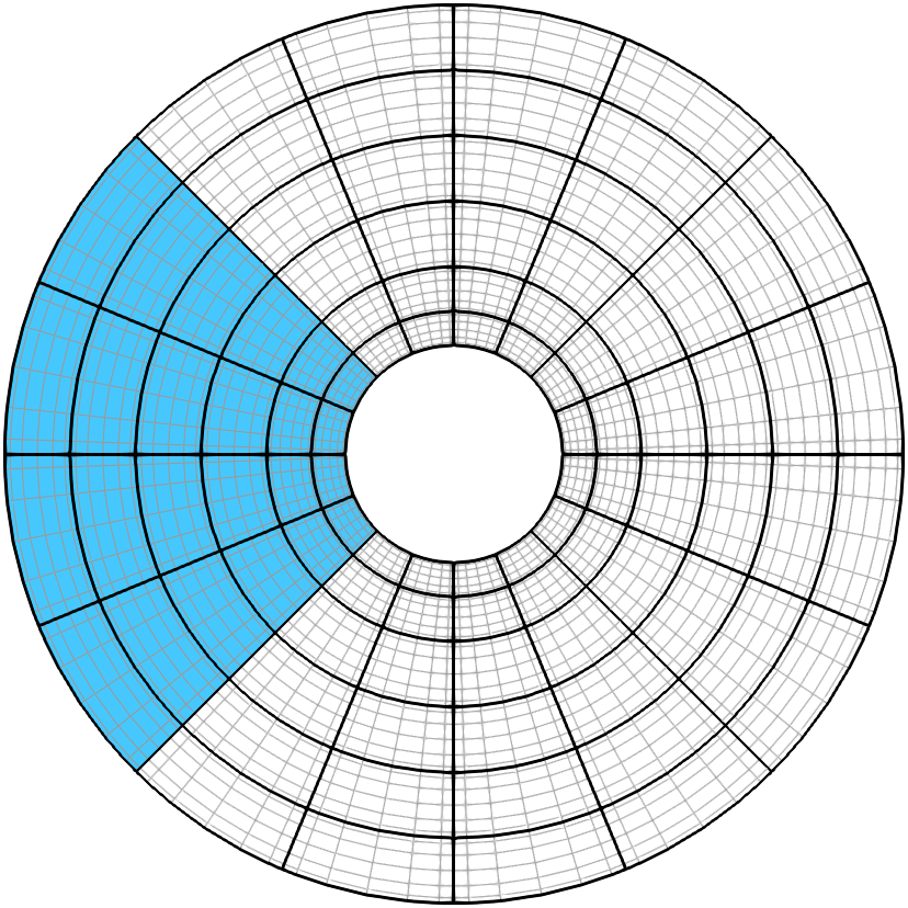
Figure 2: An illustration of a slice through the computational domain used in the evolutions of single black holes described in this paper. Six regions, each in the shape of a deformed cube, combine to cover the volume of a spherical shell, with the inner boundary (the excision surface) inside the black hole’s apparent horizon. The six regions are themselves refined radially and angularly into smaller deformed cubes. One of the six regions is shown in blue for clarity.

3.1.1 Kerr-Schild coordinates

We first evolve a single black hole in Kerr-Schild coordinates from Kerr-Schild initial data. The inner radius of the computational domain is $r_{\mathrm{in}}=r_{\mathrm{exc}}=1.8M$. In this case there are no coordinate dynamics, so a feedback control system is not necessary, though it is enabled in the simulations presented here. The left panel of figure 3 shows the gauge constraint $\mathcal{C}_{a}$ and the 3-index constraint $\mathcal{C}_{iab}$ as a function of time for several different resolutions. We evolve the lowest resolution to time $t=10,000M$ to assess long-term stability, and we evolve the medium and high resolutions to assess convergence. To limit the computational cost of these tests, we choose to evolve the medium and high resolutions only to time $t=2,000M$. All simulations are stable to time $t=2000M$, and the lowest resolution remains stable to $t=10,000M$. The amount of violation of the gauge constraint $\mathcal{C}_{a}$ and the 3-index constraint $\mathcal{C}_{iab}$ is indicative of the overall constraint violation in the simulation. In this evolution, the constraints remain constant, and they decrease exponentially with increasing $p$-refinement (that is, increasing points per cell per dimension), as expected.

The right panel of figure 3 demonstrates long-term stability and convergence for the same setup but with a black hole of dimensionless spin $\chi\equiv S/M^{2}=0.8$ (with $r_{\mathrm{in}}=r_{\mathrm{exc}}=1.57M$). Again, we see that the constraints remain constant and convergence exponentially with increasing $p$-refinement.

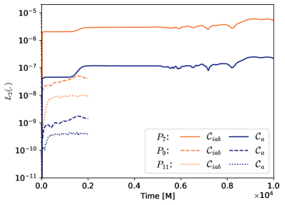
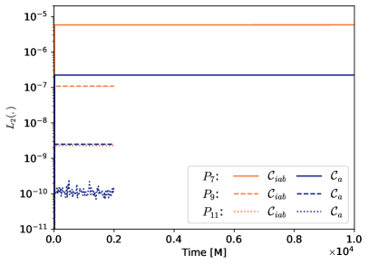
Figure 3: Constraint violations for single black hole evolutions in Kerr-Schild coordinates with Kerr-Schild initial data. We evolve the lowest resolution to time $t=10,000M$ to demonstrate long term stability and evolve two higher resolutions to time $t=2,000M$ to assess convergence with spatial resolution. Left: Non-spinning black hole. Right: Spinning black-hole with dimensionless spin $\chi=S/M^{2}=0.8$.

3.1.2 Harmonic coordinates

Next, we evolve a single black hole in harmonic gauge $H_{a}=0$ using initial data also in harmonic gauge. Here, $r_{\mathrm{in}}=r_{\mathrm{exc}}=0.9M$. The absolute and relative time stepper tolerances for the highest resolution of this test case are $10^{-10}$ and $10^{-8}$, respectively. Again, since the initial data and evolution use the same gauge there are no gauge dynamics. The left panel of figure 4 shows the gauge constraint $\mathcal{C}_{a}$ and the 3-index constraint $\mathcal{C}_{iab}$ as a function of time for several different resolutions. We evolve the lowest resolution to time $t=10,000M$ to assess stability and two higher resolutions to time $t=5,000M$ to assess convergence. The constraints again remain constant, and they decrease exponentially with increasing $p$-refinement.

As a first test of the control system, we evolve a Kerr-Schild black hole in harmonic coordinates. The inner radius of the domain again is $r_{\mathrm{in}}=r_{\mathrm{exc}}=1.8M$. The differing gauge choices in the initial data and evolution create coordinate dynamics that cause the BH horizon to shrink. The control system (§2.7) must decrease the radius of the excision surface smoothly and precisely to avoid incoming characteristic speeds, so that the problem remains well-posed and the code does not terminate. The right panel of figure 4 shows constraint violations over time for three resolutions. All evolutions are stable, and the constraint violations converge away. However, the constraints remain larger until after time $1,000M$. We suspect this is caused by initial gauge dynamics, i.e., by time-dependent, outward-moving coordinate effects that travel outward until exiting the domain through the outer boundary at $r_{\mathrm{out}}=1,000M$.

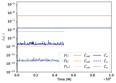
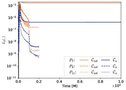
Figure 4: Constraint violations for single black hole evolutions in harmonic coordinates. We evolve the lowest resolution to time $t=10,000M$ to demonstrate long term stability and evolve two higher resolutions to an earlier time to assess convergence with spatial resolution. Left: Analytic initial data is in harmonic coordinates. Higher resolutions evolved to $t=5,000M$. The highest resolution has $10\times$ tighter time stepper tolerances. Right: Analytic initial data is in Kerr-Schild coordinates. Higher resolutions evolved to $t=2,000M$. The difference between the initial data and evolution gauge causes non-trivial dynamics.

3.1.3 Damped harmonic coordinates

Our final single-black-hole test consists of evolving Kerr-Schild analytic initial data in damped harmonic gauge with $r_{\mathrm{in}}=r_{\mathrm{exc}}=1.8M$. The left panel of figure 5 shows the constraints as a function of time for several different resolutions. Just as in the harmonic gauge case, the non-trivial gauge dynamics cause larger constraint violations until after one light-crossing time to the outer boundary of $r_{\mathrm{out}}=1,000M$. The evolutions are stable and converge with increasing resolution. We also repeated this evolution but for a black hole with a dimensionless spin of $\chi=0.8$ and $r_{\mathrm{in}}=r_{\mathrm{exc}}=0.57M$. We show the constraint violations in the right panel of figure 5. Again we see stable evolutions and exponential convergence with increasing $p$-refinement.

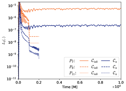
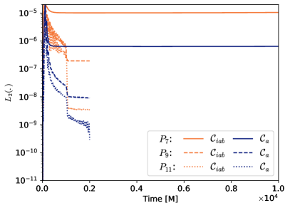
Figure 5: Constraint violations for single black hole evolutions in damped harmonic coordinates with Kerr-Schild initial data. We evolve the lowest resolution to time $t=10,000M$ to demonstrate long term stability and evolve two higher resolutions to time $t=2,000M$ to assess convergence with spatial resolution. Left: Non-spinning black hole. Right: Spinning black-hole with dimensionless spin $\chi=S/M^{2}=0.8$.

3.2 Gauge wave

As a final test of convergence and stability, we evolve analytic initial data consisting of a gauge wave in flat spacetime, a test conceived in [66] as part of a “standard testbed” for NR codes. Physically, the solution is equivalent to flat spacetime, but the chosen coordinates include a sinusoidal traveling wave that introduces time-dependence, with a line element given by

$$ds^{2}=-H(t,x)\,dt^{2}+H(t,x)\,dx^{2}+dy^{2}+dz^{2},$$ (51)

where

$$H(t,x)=1-A\sin\left(\frac{2\pi\left(x-t\right)}{d}\right),$$ (52)

where $A$ and $d$ are the amplitude and wavelength of the gauge wave, which travels along the $x$-axis.

We evolve analytic initial data of this solution, using the gauge source function $H_{a}$ computed directly from the analytic initial data. We set the FOGH constraint damping parameters to $\gamma_{0}=\gamma_{2}=1$ and $\gamma_{1}=-1$. We evolve on the domain $[0,1]^{3}$ with two elements in the $x$-direction, one element in the $y$- and $z$-directions. We fix the $y$ and $z$ points per element to 6 ($P_{5}$) and perform a convergence test by running three resolutions with 15 ($P_{14}$), 18 ($P_{17}$), and 20 ($P_{19}$) points per element in the $x$ direction. We apply periodic boundary conditions in all directions. We use a sixth-order Adams-Moulton predictor-corrector time integrator. In our simulations we choose $A=0.1$ and $d=1$.

Gauge wave simulations are known to be unstable in the BSSN formulation of the Einstein equations [67], but are stable in the Z4 system [68]. However, this is not the case with the FOGH system. The left panel of figure 6 shows the $L_{2}$ norm of the 1-index and 3-index constraints as a function of time. While the lowest resolution ($P_{14}$) simulation has exponentially growing constraints, the higher resolution simulations have constant and convergent constraints. Similarly, the right panel of figure 6 shows the $L_{2}$ norm of the error in the evolved variables $g_{ab}$, $\Pi_{ab}$, and $\Phi_{iab}$ at the three resolutions. We observe stable and convergent long-term behavior. The highest resolution simulation is close to being limited by the time stepper tolerance.

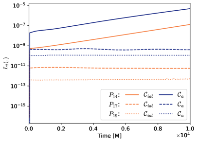
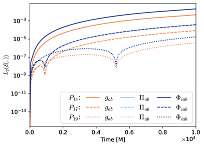
Figure 6: Results from an amplitude $0.1$ gauge wave simulation demonstrating long term stable and convergent simulations. We show simulations at three resolutions, 15, 18, and 20 grid points per element in the $x$-direction. Left: The 1-index and 3-index constraints as a function of time. The lowest resolution has exponentially growing constraints in time while the two higher resolutions have constant and convergent constraints in time. Right: Errors in the FOGH evolved variables $g_{ab}$, $\Pi_{ab}$, and $\Phi_{iab}$ at the three resolutions. We see stable and convergent long-term behavior with the errors decreasing exponentially with increasing resolution. The errors for $\Pi_{ab}$ and $\Phi_{iab}$ lie on top of each other and so only the errors for $\Phi_{iab}$ are visible.

3.3 Binary black hole inspiral, merger, and ringdown

In this section, we use SpECTRE to generate binary black hole initial data and evolve the binary through $\sim 18$ orbits of inspiral, merger, and ringdown to a final, stationary state. We then use SpECTRE’s Cauchy Characteristic Evolution (CCE) module to evolve the outgoing gravitational waves to future null infinity. We perform the simulations at three different resolutions, which we refer to as “Lev0”, “Lev1”, and “Lev2” with Lev0 being the lowest resolution and Lev2 being the highest. Each increase in resolution increases the number of points per element per dimension by one. During the inspiral, each simulation uses 4,800 elements, with Lev0, Lev1, and Lev2 having $\sim 2.6$; $\sim 3.7$; and $\sim 4.8$ million total grid points. During the ringdown, each simulation uses 7,680 elements and $\sim 10.2$, $\sim 13.3$, and $\sim 16.9$ million total grid points, respectively. All simulations use the damped harmonic gauge to prevent the lapse collapsing and $\sqrt{\gamma}$ diverging at merger. All simulations (both inspiral and ringdown) also use a fourth-order Adams-Moulton predictor-corrector time integrator with absolute and relative time stepper tolerances of $10^{-10}$ and $10^{-8}$, respectively.

The evolutions were each performed on 10 compute-nodes in the Resnick High Performance Computing Center at Caltech. Each compute node has two 28-core Intel Cascade Lake CPUs. Our Lev0, Lev1, and Lev2 evolutions cost 58,000; 71,000; and 114,000 core hours, which amounts to 104; 127; and 204 wallclock hours, and an average of 120; 80; and 43 $M$/hour during the inspiral. In a future paper, we will assess SpECTRE’s performance and scaling in more detail; our purpose for this paper is to demonstrate that SpECTRE can evolve binary black holes through inspiral, merger, and ringdown.

3.3.1 Initial data

We begin our evolutions with initial data of two equal-mass and non-spinning black holes in a quasicircular orbit. To generate the initial data we use the SpECTRE initial data module [69, 70, 71], which solves the elliptic constraint sector of the Einstein equations in the extended conformal thin sandwich (XCTS) formalism [72, 73, 74]. It uses the superposed Kerr-Schild formalism to construct a conformal background to the extended conformal thin sandwich equations based on the weighted superposition of two isolated Kerr-Schild black holes [75, 76]. The black holes are represented as excisions with negative-expansion apparent horizon boundary conditions [77, 78]. The initial data solver uses DG methods similar to those described in this article to achieve scalable and parallelizable solutions to the elliptic equations and is also open source [44, 70].

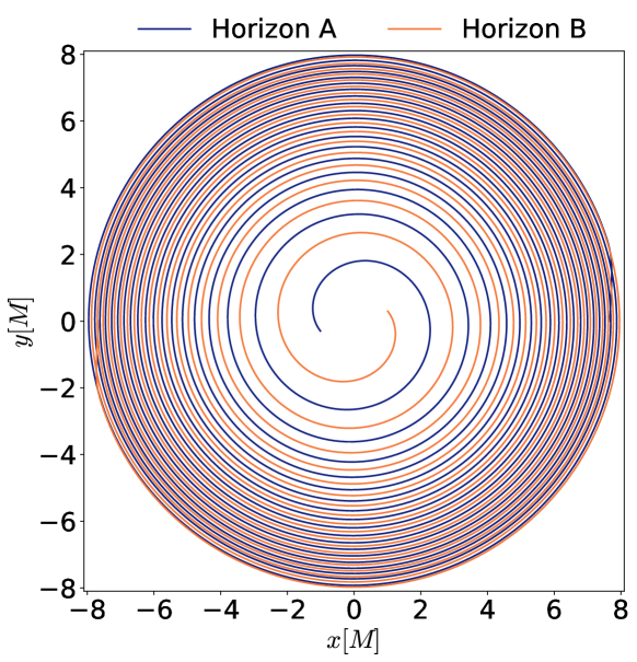
Figure 7: The trajectories of the centers of each apparent horizon during the Lev2 inspiral evolution, in the evolution’s asymptotically inertial coordinates. The coordinates $x$ and $y$ indicate the position of the black hole within the orbital plane in units of the total initial mass $M$ of the binary.

We choose an initial coordinate separation of the excision centers to be $d_{0}=15.366M$ to facilitate future comparison with the family of simulations in [79] and to place the two black holes at $\sim 18$ orbits before they merge. The masses and spins of the black holes measured on the horizons are driven to the desired values in a control loop that adjusts the initial data parameters, similar to [80]. In a second control loop we performed eccentricity reduction by evolving the initial data for a few orbits and adjusting the initial orbital parameters to iteratively reduce the eccentricity of the orbit [81, 82] to $1.1\times 10^{-3}$. The resulting initial data parameters are summarized in table 3, and a plot of the resulting inertial trajectories for Lev2 is shown in figure 7.

Table 1: Parameters used to generate the binary-black-hole initial data evolved in §3.3: in terms of the sum of the black holes’ Christodoulou masses $M=M_{1}+M_{2}$ of each black hole, the individual masses $M_{1}$ and $M_{2}$, the dimensionless spin magnitudes $|\chi_{1}|/M^{2}$ and $|\chi_{2}|/M^{2}$, the orbital eccentricity $e$, the initial coordinate separation $d_{0}$ of the horizon centers, the initial orbital angular velocity $\Omega_{0}$, and the initial expansion rate $\dot{a}_{0}$.

• $M_{1}/M$	$M_{2}/M$	$|\chi_{1}|/M^{2}$	$|\chi_{2}|/M^{2}$	$d_{0}/M$	$M\Omega_{0}$	$e$	$\dot{a}_{0}$
  0.5	0.5	$1.8\times 10^{-6}$	$4.6\times 10^{-7}$	15.366	0.0159	$1.1\times 10^{-3}$	$3.4\times 10^{-5}$

3.3.2 Computational domain decomposition

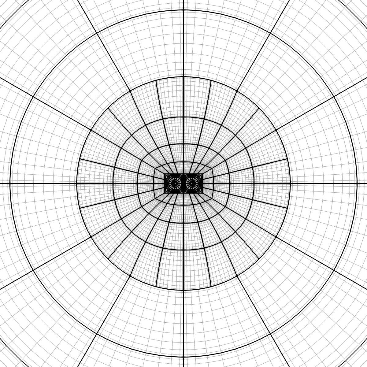
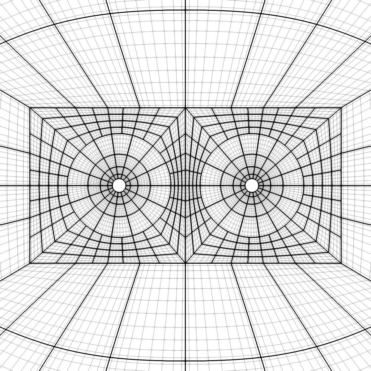
Figure 8: An illustration of the computational grid used during the inspiral. We make use of two excision regions, each region lying inside a black hole’s apparent horizon. Each excision is surrounded by a spherical shell partitioned into six deformed cubes as in figure 2. Each spherical shell is then surrounded by another shell of six deformed cubes that transition to a cubical boundary. Then the two cubes themselves are surrounded by a transitionary envelope which becomes spherical. Left: The transitionary envelope. Right: A close-up of the domain structure around the excisions. The center of each excision is offset from the center of the cube.

The numerical evolution of the GH system is performed with a DG scheme in which the physical domain of the problem is partitioned into deformed hexahedral elements with conforming boundaries. The boundaries and gridpoint distributions of an element are determined by a continuous and differentiable coordinate map applied to the logical Cartesian coordinates, which we label $\xi,\eta$ and $\zeta$, of a regular cube spanning $[-1,1]^{3}$. The maps corresponding to neighboring elements are required to be continuous but are not required to be differentiable at element boundaries. This provides the flexibility necessary to construct the complicated domains needed for binary merger simulations using DG methods. An example of the domain used during the inspiral is shown in figure 8 and an example of the ringdown domain is shown in figure 9. While the coordinate maps provide significant flexibility, we found that instabilities arise if neighboring elements differ by significantly more than a factor of two in size, placing a practical constraint on how quickly the resolution can be reduced as one moves away from the BHs.

Our computational domain is the region of space between the outer spherical boundary and the excision boundaries that remove the black hole singularities from the domain. The excision boundaries are spherical in the comoving coordinates with their sizes and shapes in the inertial coordinates informed by the size and shape of the apparent horizons (§2.7). At merger the apparent horizons of the inspiraling black holes become enveloped by a single common apparent horizon. We handle the different number of excision boundaries during the inspiral and ringdown by having distinct domains for each. At merger we interpolate data from the inspiral domain that has two excision boundaries to the ringdown domain that has one excision boundary. We describe each domain below.

The inspiral domain:

The inspiral domain is more complicated than the ringdown domain. This is because of the complexity of having two excisions. During the inspiral we must tile a two-excision domain with conforming hexahedra. Our solution to this tiling problem makes use of 44 element collections grouped into two radial and two “biradial” layers. Our description of the domain decomposition starts at the excision surfaces and extends radially outward.

The first layer consists of six wedges composing the spherical shell surrounding each excision. Each wedge is subdivided into multiple elements. The black holes are located on the $x$-axis at $x\sim\pm 7.683M$ with an excision radius of $r_{\mathrm{exc}}\sim 0.792M$. The shell around each black hole has an outer radius of $6M$. For a fixed target accuracy, distributing the grid points logarithmically in radius and equiangularly [83, 84] in angles significantly reduces computational cost.

The second layer uses a set of wedges that wrap the shells around each black hole in a cubical shell, as seen in figure 8. A consequence of the decreasing separation between the two black holes during the inspiral is that the size of the excision within each cube grows as the simulation progresses. Since we only deform the region inside the cubes to conform to the shape of the apparent horizons, the simulation will fail if the apparent horizons grow beyond the cube boundaries. We remedy this by decoupling the excision center from the center of the cube (see the right panel of figure 8), effectively increasing the size of the cube relative to the size of the excision by a constant factor that is sufficient to keep the apparent horizons within the cubes throughout the simulation. This generalized map is crucial for robust inspiral and merger simulations.

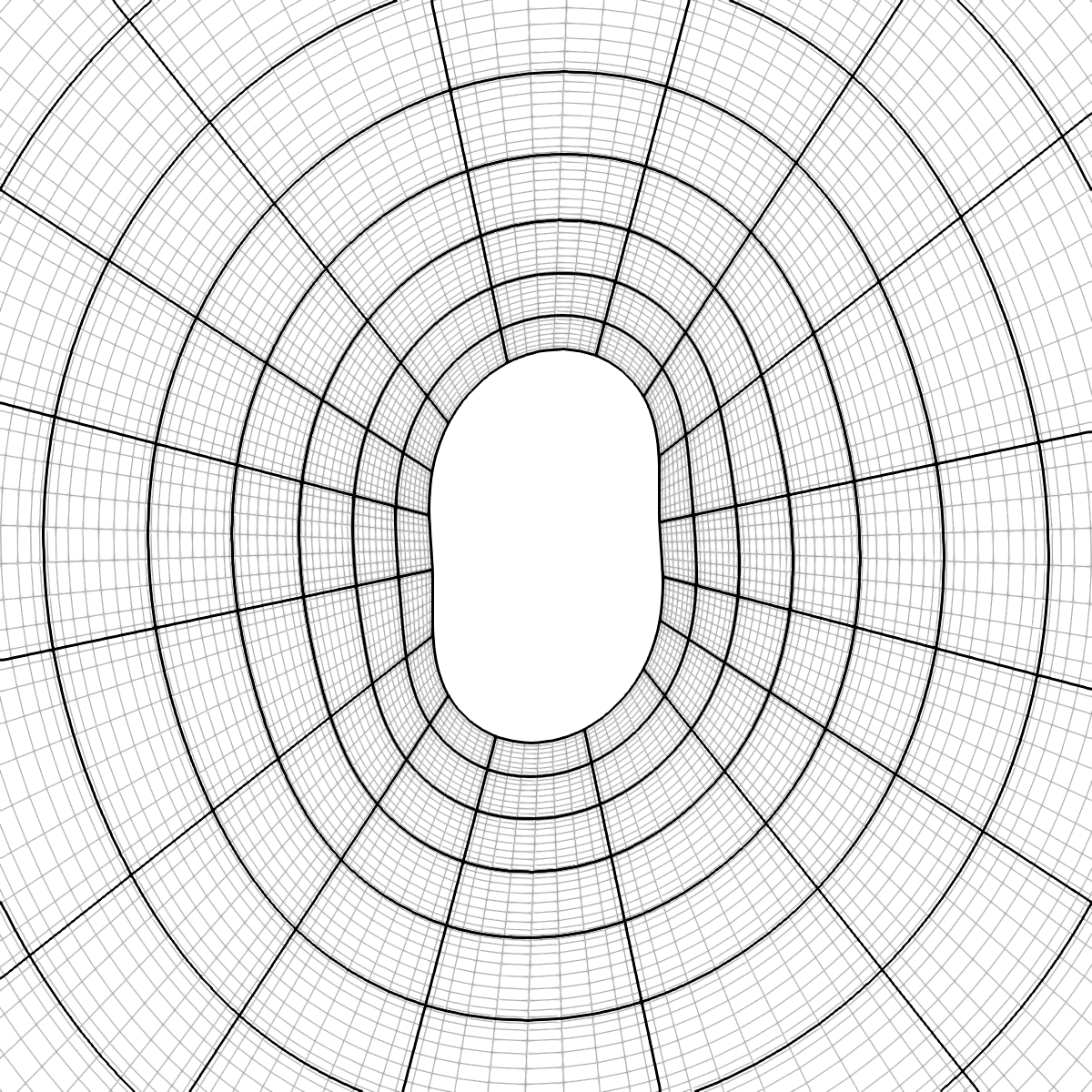
Figure 9: An image of the ringdown domain. After a common horizon is found, the evolution is regridded onto a domain with a single excision as in figure 2. Additional time-dependent maps are used to deform the excision’s spherical shape into one that corresponds to the common horizon shape.

The third layer consists of the elements surrounding the cubes around each black hole (layers 1 and 2). We refer to this region, which extends from $r\sim 18M$ to $r=100M$, as the “envelope”. This layer serves to transition the grid point distributions from what is used near the black holes to the distribution that is used in the wave zone. We use a logarithmic map in the radial direction and we interpolate between a “biradial” equiangular map used for two excisions and a “radial” equiangular map suited for the spherical outer boundary.

The fourth and final layer is a spherical shell extending from the end of the envelope ($r=100M$) to the outer boundary at $r=600M$. This shell uses a linear distribution in the radial direction and an equiangular distribution in the angular directions. Since the GW wavelength is constant in radius, a linear distribution is necessary to avoid under resolving the waves. In production quality simulations we expect to place the outer boundary at $r=1,500M$, since in SpEC simulations we observe a center-of-mass drift caused by the gauge boundary condition. Errors in the gauge boundary condition fall off as $\sim 1/r^{2}$. We find that the drift is larger for longer simulations, but this can be compensated for with a larger outer boundary. Since we use CCE to extract the gravitational waves, a large domain for wave extraction is not required.

In addition to the hexahedral maps that partition the domain, we also globally apply rotation and expansion maps that track the angular, radial, and center of mass motion of the binary system.

The ringdown domain:

The ringdown domain is a single excision domain used after a common apparent horizon has formed. An example of this domain is shown in figure 9. It is similar in structure to the domain used in the single black hole tests in §3.1. We use a logarithmic radial map from the excision surface to $r=50M$ and use a linear spacing further away to resolve the gravitational waves. We used an equidistant map instead of an equiangular map in the angular directions. A significant challenge compared to the single black hole evolution is that the time-dependent maps used during ringdown must be initialized from, and matched to, the corresponding time-dependent maps in the inspiral. The rotation and expansion maps are matched and then decay exponentially to being time-independent. Most challenging are the shape and size maps. For the shape map we perform a least squares fit in time to the spherical harmonic coefficients of the common horizon found during the inspiral. We fit to 100 times, and then initialize the shape map by evaluating the fit at the transition time. For the size map, we manually specify an excision radius $r_{\mathrm{exc}}=1.45$ and gave the excision surface an initial outward velocity of 1.0.

3.3.3 Constraint damping

Based on our experience evolving binary black holes in SpEC, we use a superposition of three Gaussians and a constant for $\gamma_{0}$ and $\gamma_{2}$, and a single Gaussian plus a constant for $\gamma_{1}$. See (4) for how the constraint damping terms appear in the evolution equations. The motivation for the different Gaussians is to increase the constraint damping near each black hole, which requires the Gaussians to move with the black holes as they inspiral. In SpEC and SpECTRE we achieve this by making the Gaussians functions of the comoving “grid frame” coordinates $x^{\bar{\imath}}$. As the black holes inspiral, their coordinate radius increases in the comoving $x^{\bar{\imath}}$ coordinates, which means the width $w$ of the Gaussian must also increase by the same amount. Increasing the width is achieved by dividing the width by the expansion factor $E(t)$, which starts at $1$ and decreases as the black holes inspiral. The specific form of the damping parameters we use is

$$\gamma_{0}(t,x^{\bar{\imath}}) = \gamma_{2}(t,x^{\bar{\imath}})=C+\sum_{I=0}^{2}A_{I}\exp\left[-\left(\frac{\bar{r}_{I}}{\bar{w}_{I}/E(t)}\right)^{2}\right],$$ (53)

$$\gamma_{1}(t,x^{\bar{\imath}}) = C+A_{0}\exp\left[-\left(\frac{\bar{r}_{0}}{\bar{w}_{0}}\right)^{2}\right],$$ (54)

where $C$ is a constant, $A_{I}$ are the amplitudes of the Gaussians, $\bar{r}_{I}$ are the grid-frame radii from the center of each Gaussian, and $\bar{w}_{I}$ are the widths of the Gaussians in the grid frame. Table 2 shows the parameters during the inspiral and table 3 shows them during the ringdown. In the grid frame the black holes are always located on the $\bar{x}$-axis so we only specify the grid frame $\bar{x}$-coordinate at which each Gaussian is centered, denoted by $\bar{x}^{C}$ in tables 2 and 3.

Table 2: Parameters for the Gaussians that make up the constraint damping functions during the inspiral. See (53) and (54) for how the coefficients appear in the functional form of the constraint damping parameters.

• 	$C$	$A_{0}$	$\bar{w}_{0}$	$\bar{x}_{0}^{C}$	$A_{1}$	$\bar{w}_{1}$	$\bar{x}_{1}^{C}$	$A_{2}$	$\bar{w}_{2}$	$\bar{x}_{2}^{C}$
  $\gamma_{0}$	$0.01/M$	$0.75/M$	38.415	0	$8/M$	3.5	7.683	$8/M$	3.5	-7.683
  $\gamma_{1}$	$-0.999/M$	$0.999/M$	$10d_{0}$	–	–	–	–	–	–	–
  $\gamma_{2}$	$0.01/M$	$0.75/M$	38.415	0	$8/M$	3.5	7.683	$8/M$	3.5	-7.683

Table 3: Parameters for the Gaussians that make up the constraint damping functions during the ringdown. See (53) and (54) for how the coefficients appear in the functional form of the constraint damping parameters.

• 	$C$	$A_{0}$	$\bar{w}_{0}$	$\bar{x}_{0}^{C}$	$A_{1}$	$\bar{w}_{1}$	$\bar{x}_{1}^{C}$	$A_{2}$	$\bar{w}_{2}$	$\bar{x}_{2}^{C}$
  $\gamma_{0}$	$0.01/M$	$1.0/M$	100	0	$7/M$	2.5	0	–	–	–
  $\gamma_{1}$	$-0.999999/M$	–	–	–	–	–	–	–	–	–
  $\gamma_{2}$	$0.001/M$	$0.1/M$	100	0	$7/M$	2.5	0	–	–	–

3.3.4 Constraint violations

Figure 10 shows the constraint energy $\mathcal{E}$ (see (19)) as function of time at each resolution. Experience from SpEC suggests that the initial, rapid growth in $\mathcal{E}$ is caused by not resolving the initial data’s rapid relaxation and emission of spurious, high-frequency “junk” gravitational radiation at the start of the simulation. Resolving the junk radiation is computationally expensive and generally not done in NR evolutions of binary black holes. After the initial growth of constraint violation damps away, the constraints converge exponentially with increasing $p$-refinement. The constraints grow sharply near the time of merger, as the black holes become more distorted by each others’ tidal gravity, causing the solution to be less resolved by our fixed computational mesh. We anticipate that future SpECTRE simulations using adaptive mesh refinement will improve the behavior of the constraints near the time of merger.

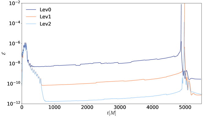
Figure 10: L2-norm of the constraint energy $\mathcal{E}$ (see (19)) over the entire computational domain for evolutions of an equal-mass, non-spinning, binary black hole at low (“Lev0”), medium (“Lev1”), and high (“Lev2”) spatial resolution, as a function of time $t$ in units of the initial total mass $M$. The peak of the constraint energy for each resolution is when we transition to the ringdown grid. We see exponential convergence with resolution except at merger and early ringdown, where adaptive mesh refinement will be necessary to resolve the additional dynamics.

After the merger, as the remnant black hole rings down, the constraint violations decrease to much smaller values again. When the black hole has settled to its final stationary state, the constraint violations continue to slowly decrease in time. Because the ringdown constraints in the highest resolution are not smaller than those with the medium spatial resolution, we suspect that the numerical error is dominated not by spatial resolution in the ringdown but by some other factor. One possibility is the time-stepping accuracy during the late inspiral and ringdown. We leave a careful study of this, including improvements to the domain decomposition and use of adaptive mesh refinement during the ringdown, to future work.

3.3.5 Apparent horizons

Another way of measuring the accuracy of BBH simulations is to track the masses and spins of the BHs. We measure masses and spins on the individual apparent horizons during the inspiral and merger and on the common apparent horizon during ringdown. The irreducible mass, defined as $M_{\mathrm{irr}}\equiv\sqrt{A/16\pi}$, where $A$ is the surface area of the apparent horizon, should be monotonically increasing. Thus, any decreases in $M_{\mathrm{irr}}$ can be viewed as a measure of the numerical error in the simulation. Another useful metric is the Christodoulou mass $M_{\mathrm{Ch}}\equiv\sqrt{M_{\mathrm{irr}}^{2}+S^{2}/4M_{\mathrm{irr}}^{2}}$, which includes both the irreducible mass and rotational kinetic energy. The dimensionless spin $\chi=S/M_{\mathrm{Ch}}^{2}$ measures the spin in terms of approximate rotational Killing vectors, as discussed in Appendix A of [75]. For equal-mass non-spinning simulations $M_{\mathrm{irr}}$ and $M_{\mathrm{Ch}}$ should remain constant until merger, while $\chi$ should remain identically zero. Deviations from this behavior help quantify numerical errors in the simulation.

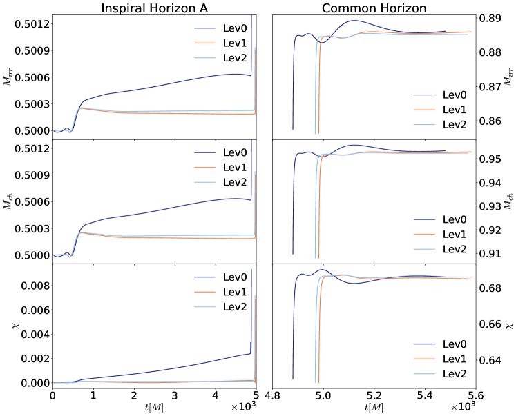
Figure 11: Apparent horizon masses and spins as a function of time. The left column shows the irreducible mass $M_{\rm irr}$, Christodoulou mass $M_{\rm ch}$, and dimensionless spin angular momentum $\chi\equiv S/M_{\rm ch}^{2}$ for one of the individual apparent horizons during inspiral, as a function of time $t$ in units of the total initial Christodoulou mass $M$. The right column shows the same quantities during the ringdown for the common apparent horizon. We see convergence with increasing resolution, specifically that the Lev1 and Lev2 evolutions track each other more closely than the Lev0 and Lev1 simulations.

Figure 11 shows $M_{\mathrm{irr}}$, $M_{\mathrm{Ch}}$, and $\chi$ during the inspiral and ringdown. We find that the masses and spins over time are convergent, in the sense that the difference between Lev0 and Lev1 is greater than the difference between Lev1 and Lev2. During the inspiral, after the initial transient, the masses and spins remain more constant in time as resolution increases, until sharp gains near the time of merger as the black holes gain energy and angular momentum. During the ringdown, the masses and spins relax to final, constant values, as expected. The final Christodoulou mass $M_{\rm ch}=0.952$ differs from the initial Christodoulou mass ($M_{\rm ch}=1$) by 4.8%, and the final spin is $0.686$. Both values are consistent with the fitting formulas in [79], tuned using SpEC evolutions of equal-mass, equal-aligned-spin binary black holes.

3.3.6 Gravitational waveforms

We compute gravitational waveforms using Cauchy-Characteristic Evolution (CCE) [85, 86, 87, 88, 46], using the SpECTRE implementation of CCE [45]. This method utilizes an additional characteristic evolution code, the one described in [45], that solves the full Einstein equations on a set of outgoing null slices that extend from some inner worldtube all the way to future null infinity. Boundary conditions on the worldtube are provided by the interior Cauchy evolution, in this case also done with SpECTRE. For the characteristic evolution, there is freedom to choose one complex function on the initial null slice, which encodes the initial incoming radiation. We set it according to equation (16) of [45]. From the characteristic evolution, one can compute the gravitational-wave strain and all five Weyl scalars at future null infinity. Gravitational waveforms computed via CCE are in a well-defined gauge modulo Bondi-van der Burg-Metzner-Sachs (BMS) transformations [89, 90], which are extensions of Poincaré transformations and correspond to symmetries of asymptotically flat spacetimes at future null infinity. The raw output from CCE is in an effectively random BMS frame, so to completely fix the gauge, it is necessary to perform a BMS transformation [91]. We choose to transform waveforms into the superrest frame of the inspiral [92, 93], which can be thought of as the BMS extension of a frame in which the binary is at rest during the inspiral. We find the BMS transformation to map to this frame using data from the strain and Weyl scalars over the time window $[1800M,2200M]$. See [91] and references therein for an in-depth review of BMS frame fixing.

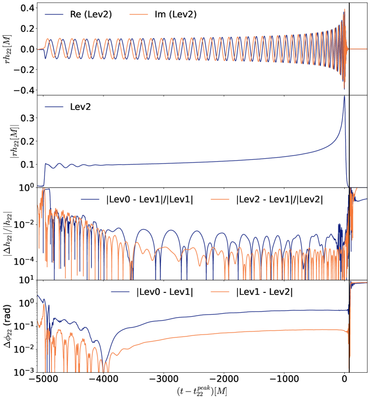
Figure 12: The $\ell=m=2$ spin-weighted spherical-harmonic mode of the gravitational waves, computed using Cauchy Characteristic Evolution (CCE) and frame-fixed using the Python package scri, with a worldtube radius of $200M$, where $M$ is the total initial Christodoulou mass. From top to bottom, as a function of retarded time $t-t^{\rm peak}_{22}$, the panels show i) the real and imaginary part of the strain $rh_{22}/M$; ii) the amplitude $|rh_{22}/M|$ at the highest spatial resolution; iii) the fractional amplitude difference $|\Delta h_{22}|/|h_{22}|$, defined as the magnitude of the $\ell=m=2$ amplitude difference between two spatial resolutions, divided by the magnitude of the higher spatial resolution’s amplitude; iv) the difference in phase $\Delta\phi_{22}$, defined as the difference between the $\ell=m=2$ gravitational-wave phase at two different spatial resolutions, with each phase offset such that the phase vanishes at $t-t_{22}^{\rm peak}=-4000M$. The vertical black lines shows where the amplitude goes below $\sim 10^{-3}$.

Figure 12 shows the leading-order $\ell=m=2$ spin-weighted spherical harmonic mode of the gravitational-wave strain as a function of retarded time $t$. To estimate the accuracy of the waveforms, we first apply a time shift $t_{22}^{\rm peak}$ so that the peak amplitudes at each spatial resolution occur at the same shifted time. Then, we apply a constant phase offset such that the gravitational-wave phase of the $\ell=m=2$ mode vanishes at time $t-t_{22}^{\rm peak}=-4000M$. This time was chosen as an early time after most of the initial, spurious “junk” radiation (especially visible in the amplitude at early times) has been emitted. This junk radiation is characteristically different than the junk radiation seen in figure 10. The junk radiation in figure 12 is of a lower frequency and is due to our choice of data on the initial null slice. It is an active area of research to improve data on the initial null slice.

We choose to post-process the data in this way because it enables us to transform each simulation to some reasonable BMS frame without using information from the other simulations. As a result, we can perform more meaningful convergence tests, since the output from each simulation is independent of every other. While one could obtain better agreement between different resolutions by finding the BMS transformation which minimizes the residual between the simulations’ waveforms, this would go beyond computing a convergence error, because the frame of one simulation is determined by the other.

Finally, we interpolate the amplitudes and phases at each spatial resolution onto a common set of times and take differences, estimating the numerical error of a spatial resolution in terms of its difference with the next highest spatial resolution. We find that between time $t-t_{22}^{\rm peak}=-4000M$ and merger time $t-t_{22}^{\rm peak}=0$, the amplitude and phase differences decrease with increasing resolution, as expected, with the medium and high resolution differing in amplitude by $0.04\%$ at time of merger. During the window between $t-t_{22}^{\rm peak}=-4000M$ and $t=t_{22}^{\rm peak}$, the medium and high spatial resolutions accumulate $0.06$ radians of phase error. After merger time, the fractional amplitude and phase errors grow, which is expected, because the amplitude itself is exponentially falling to zero, making determining the phase accurately increasingly challenging.

4 Conclusion

We present the first inspiral-merger-ringdown simulations of two binary black holes using discontinuous Galerkin methods. We use the open-source numerical relativity code SpECTRE [44] to perform all simulations. These include several long-term stability and accuracy tests, e.g. evolutions of a single black hole in Kerr-Schild, harmonic, and damped harmonic gauge, as well as a long-term stable gauge wave simulation. All simulations demonstrate the expected exponential convergence.

The binary black hole simulation is of the last 18 orbits before merger of an equal mass non-spinning binary. We extract gravitational waveforms at future null infinity using SpECTRE’s CCE module. We observe exponential convergence in the constraint violations with increasing resolution, and demonstrate convergence in amplitude and phase of the $\ell=m=2$ mode of the gravitational wave strain. Our medium and high resolution simulations run at 80 and 43 $M$/hour on ten 56-core Intel Cascade Lake nodes. The simulations presented here are the first binary merger simulations where the initial data, evolution, and wave extraction are all performed using the open-source code SpECTRE.

While the results here present a milestone for SpECTRE simulations, several further advancements are necessary to enable building catalogs for future gravitational wave detectors. These fall in one of four categories: i) performance improvements like using adaptive mesh refinement, dynamic load balancing, and GPU support; ii) robustness and parameter space improvements like ensuring that high-spin, high-mass-ratio, and eccentric simulations can be performed robustly without hand tuning; iii) automation infrastructure that allows a single user to run hundreds of simulations, such as automatically restarting failed simulations, automatically transitioning from inspiral to ringdown, and automatically running CCE after the Cauchy simulation completes; and iv) improving documentation and tutorials to make the code more accessible to the broader community. These will allow SpECTRE to outperform our current code SpEC and to be more useful to the broader numerical-relativity community.

References

References

- [1] R. Abbott et al. GWTC-3: Compact Binary Coalescences Observed by LIGO and Virgo during the Second Part of the Third Observing Run. Phys. Rev. X, 13(4):041039, 2023.
- [2] Luc Blanchet. Post-Newtonian theory for gravitational waves. Living Rev. Rel., 27(1):4, 2024.
- [3] Frans Pretorius. Evolution of binary black hole spacetimes. Phys. Rev. Lett., 95:121101, 2005.
- [4] Manuela Campanelli, C. O. Lousto, P. Marronetti, and Y. Zlochower. Accurate evolutions of orbiting black-hole binaries without excision. Phys. Rev. Lett., 96:111101, 2006.
- [5] John G. Baker, Joan Centrella, Dae-Il Choi, Michael Koppitz, and James van Meter. Gravitational wave extraction from an inspiraling configuration of merging black holes. Phys. Rev. Lett., 96:111102, 2006.
- [6] Matthew D. Duez and Yosef Zlochower. Numerical Relativity of Compact Binaries in the 21st Century. Rept. Prog. Phys., 82(1):016902, 2019.
- [7] Harald P. Pfeiffer. Numerical simulations of compact object binaries. Class. Quant. Grav., 29:124004, 2012.
- [8] James Healy, Carlos O. Lousto, Yosef Zlochower, and Manuela Campanelli. The RIT binary black hole simulations catalog. Class. Quant. Grav., 34(22):224001, 2017.
- [9] James Healy, Carlos O. Lousto, Jacob Lange, Richard O’Shaughnessy, Yosef Zlochower, and Manuela Campanelli. Second RIT binary black hole simulations catalog and its application to gravitational waves parameter estimation. Phys. Rev. D, 100(2):024021, 2019.
- [10] James Healy and Carlos O. Lousto. Third RIT binary black hole simulations catalog. Phys. Rev. D, 102(10):104018, 2020.
- [11] James Healy and Carlos O. Lousto. Fourth RIT binary black hole simulations catalog: Extension to eccentric orbits. Phys. Rev. D, 105(12):124010, 2022.
- [12] Karan Jani, James Healy, James A. Clark, Lionel London, Pablo Laguna, and Deirdre Shoemaker. Georgia Tech Catalog of Gravitational Waveforms. Class. Quant. Grav., 33(20):204001, 2016.
- [13] Deborah Ferguson et al. Second MAYA Catalog of Binary Black Hole Numerical Relativity Waveforms. 9 2023.
- [14] Abdul H. Mroue et al. Catalog of 174 Binary Black Hole Simulations for Gravitational Wave Astronomy. Phys. Rev. Lett., 111(24):241104, 2013.
- [15] Michael Boyle et al. The SXS Collaboration catalog of binary black hole simulations. Class. Quant. Grav., 36(19):195006, 2019.
- [16] M. Punturo, M. Abernathy, F. Acernese, B. Allen, N. Andersson, K. Arun, F. Barone, B. Barr, M. Barsuglia, M. Beker, N. Beveridge, S. Birindelli, S. Bose, L. Bosi, S. Braccini, C. Bradaschia, T. Bulik, E. Calloni, G. Cella, E. Chassande Mottin, S. Chelkowski, A. Chincarini, J. Clark, E. Coccia, C. Colacino, J. Colas, A. Cumming, L. Cunningham, E. Cuoco, S. Danilishin, K. Danzmann, G. De Luca, R. De Salvo, T. Dent, R. De Rosa, L. Di Fiore, A. Di Virgilio, M. Doets, V. Fafone, P. Falferi, R. Flaminio, J. Franc, F. Frasconi, A. Freise, P. Fulda, J. Gair, G. Gemme, A. Gennai, A. Giazotto, K. Glampedakis, M. Granata, H. Grote, G. Guidi, G. Hammond, M. Hannam, J. Harms, D. Heinert, M. Hendry, I. Heng, E. Hennes, S. Hild, J. Hough, S. Husa, S. Huttner, G. Jones, F. Khalili, K. Kokeyama, K. Kokkotas, B. Krishnan, M. Lorenzini, H. Lück, E. Majorana, I. Mandel, V. Mandic, I. Martin, C. Michel, Y. Minenkov, N. Morgado, S. Mosca, B. Mours, H. Müller–Ebhardt, P. Murray, R. Nawrodt, J. Nelson, R. Oshaughnessy, C. D. Ott, C. Palomba, A. Paoli, G. Parguez, A. Pasqualetti, R. Passaquieti, D. Passuello, L. Pinard, R. Poggiani, P. Popolizio, M. Prato, P. Puppo, D. Rabeling, P. Rapagnani, J. Read, T. Regimbau, H. Rehbein, S. Reid, L. Rezzolla, F. Ricci, F. Richard, A. Rocchi, S. Rowan, A. Rüdiger, B. Sassolas, B. Sathyaprakash, R. Schnabel, C. Schwarz, P. Seidel, A. Sintes, K. Somiya, F. Speirits, K. Strain, S. Strigin, P. Sutton, S. Tarabrin, A. Thüring, J. van den Brand, C. van Leewen, M. van Veggel, C. van den Broeck, A. Vecchio, J. Veitch, F. Vetrano, A. Vicere, S. Vyatchanin, B. Willke, G. Woan, P. Wolfango, and K. Yamamoto. The Einstein Telescope: a third-generation gravitational wave observatory. Classical and Quantum Gravity, 27(19):194002, October 2010.
- [17] Matthew Evans et al. A Horizon Study for Cosmic Explorer: Science, Observatories, and Community. 9 2021.
- [18] Pau Amaro-Seoane, Heather Audley, Stanislav Babak, John Baker, Enrico Barausse, Peter Bender, Emanuele Berti, Pierre Binetruy, Michael Born, Daniele Bortoluzzi, Jordan Camp, Chiara Caprini, Vitor Cardoso, Monica Colpi, John Conklin, Neil Cornish, Curt Cutler, Karsten Danzmann, Rita Dolesi, Luigi Ferraioli, Valerio Ferroni, Ewan Fitzsimons, Jonathan Gair, Lluis Gesa Bote, Domenico Giardini, Ferran Gibert, Catia Grimani, Hubert Halloin, Gerhard Heinzel, Thomas Hertog, Martin Hewitson, Kelly Holley-Bockelmann, Daniel Hollington, Mauro Hueller, Henri Inchauspe, Philippe Jetzer, Nikos Karnesis, Christian Killow, Antoine Klein, Bill Klipstein, Natalia Korsakova, Shane L Larson, Jeffrey Livas, Ivan Lloro, Nary Man, Davor Mance, Joseph Martino, Ignacio Mateos, Kirk McKenzie, Sean T McWilliams, Cole Miller, Guido Mueller, Germano Nardini, Gijs Nelemans, Miquel Nofrarias, Antoine Petiteau, Paolo Pivato, Eric Plagnol, Ed Porter, Jens Reiche, David Robertson, Norna Robertson, Elena Rossi, Giuliana Russano, Bernard Schutz, Alberto Sesana, David Shoemaker, Jacob Slutsky, Carlos F. Sopuerta, Tim Sumner, Nicola Tamanini, Ira Thorpe, Michael Troebs, Michele Vallisneri, Alberto Vecchio, Daniele Vetrugno, Stefano Vitale, Marta Volonteri, Gudrun Wanner, Harry Ward, Peter Wass, William Weber, John Ziemer, and Peter Zweifel. Laser Interferometer Space Antenna. arXiv e-prints, page arXiv:1702.00786, February 2017.
- [19] Michael Pürrer and Carl-Johan Haster. Gravitational waveform accuracy requirements for future ground-based detectors. Phys. Rev. Res., 2(2):023151, 2020.
- [20] Deborah Ferguson, Karan Jani, Pablo Laguna, and Deirdre Shoemaker. Assessing the readiness of numerical relativity for LISA and 3G detectors. Phys. Rev. D, 104(4):044037, 2021.
- [21] Aasim Jan, Deborah Ferguson, Jacob Lange, Deirdre Shoemaker, and Aaron Zimmerman. Accuracy limitations of existing numerical relativity waveforms on the data analysis of current and future ground-based detectors. Phys. Rev. D, 110(2):024023, 2024.
- [22] Hengrui Zhu, Jacob Fields, Francesco Zappa, David Radice, James Stone, Alireza Rashti, William Cook, Sebastiano Bernuzzi, and Boris Daszuta. Performance-Portable Numerical Relativity with AthenaK. 9 2024.
- [23] https://www.black-holes.org/SpEC.html.
- [24] J.S. Hesthaven, S. Gottlieb, and D. Gottlieb. Spectral Methods for Time-Dependent Problems. Cambridge University Press, Cambridge, UK, 2007.
- [25] Alireza Rashti, Francesco Maria Fabbri, Bernd Brügmann, Swami Vivekanandji Chaurasia, Tim Dietrich, Maximiliano Ujevic, and Wolfgang Tichy. New pseudospectral code for the construction of initial data. Phys. Rev. D, 105(10):104027, 2022.
- [26] L. Jens Papenfort, Samuel D. Tootle, Philippe Grandclément, Elias R. Most, and Luciano Rezzolla. New public code for initial data of unequal-mass, spinning compact-object binaries. Phys. Rev. D, 104(2):024057, 2021.
- [27] Hannes R. Rüter, David Hilditch, Marcus Bugner, and Bernd Brügmann. Hyperbolic Relaxation Method for Elliptic Equations. Phys. Rev. D, 98(8):084044, 2018.
- [28] Wolfgang Tichy, Liwei Ji, Ananya Adhikari, Alireza Rashti, and Michal Pirog. The new discontinuous Galerkin methods based numerical relativity program Nmesh. Class. Quant. Grav., 40(2):025004, 2023.
- [29] David Hilditch, Andreas Weyhausen, and Bernd Brügmann. A pseudospectral method for gravitational wave collapse. Phys. Rev. D, 93(6):063006, 2016.
- [30] Marcus Bugner, Tim Dietrich, Sebastiano Bernuzzi, Andreas Weyhausen, and Bernd Brügmann. Solving 3D relativistic hydrodynamical problems with weighted essentially nonoscillatory discontinuous Galerkin methods. Phys. Rev. D, 94(8):084004, 2016.
- [31] David Hilditch, Andreas Weyhausen, and Bernd Brügmann. Evolutions of centered Brill waves with a pseudospectral method. Phys. Rev. D, 96(10):104051, 2017.
- [32] Isabel Suárez Fernández, Rodrigo Vicente, and David Hilditch. Semilinear wave model for critical collapse. Phys. Rev. D, 103(4):044016, 2021.
- [33] Maitraya K. Bhattacharyya, David Hilditch, K. Rajesh Nayak, Sarah Renkhoff, Hannes R. Rüter, and Bernd Brügmann. Implementation of the dual foliation generalized harmonic gauge formulation with application to spherical black hole excision. Phys. Rev. D, 103(6):064072, 2021.
- [34] Isabel Suárez Fernández, Sarah Renkhoff, Daniela Cors, Bernd Bruegmann, and David Hilditch. Evolution of Brill waves with an adaptive pseudospectral method. Phys. Rev. D, 106(2):024036, 2022.
- [35] Daniela Cors, Sarah Renkhoff, Hannes R. Rüter, David Hilditch, and Bernd Brügmann. Formulation improvements for critical collapse simulations. Phys. Rev. D, 108(12):124021, 2023.
- [36] Sarah Renkhoff, Daniela Cors, David Hilditch, and Bernd Brügmann. Adaptive hp refinement for spectral elements in numerical relativity. Phys. Rev. D, 107(10):104043, 2023.
- [37] Thomas W. Baumgarte, Bernd Brügmann, Daniela Cors, Carsten Gundlach, David Hilditch, Anton Khirnov, Tomáš Ledvinka, Sarah Renkhoff, and Isabel Suárez Fernández. Critical Phenomena in the Collapse of Gravitational Waves. Phys. Rev. Lett., 131(18):181401, 2023.
- [38] Krinio Marouda, Daniela Cors, Hannes R. Rüter, Florian Atteneder, and David Hilditch. Twist-free axisymmetric critical collapse of a complex scalar field. Phys. Rev. D, 109(12):124042, 2024.
- [39] Florian Atteneder, Hannes R. Rüter, Daniela Cors, Roxana Rosca-Mead, David Hilditch, and Bernd Brügmann. Boson star head-on collisions with constraint-violating and constraint-satisfying initial data. Phys. Rev. D, 109(4):044058, 2024.
- [40] Michael Dumbser, Olindo Zanotti, and Ilya Peshkov. High order discontinuous Galerkin schemes with subcell finite volume limiter and AMR for a monolithic first–order BSSNOK formulation of the Einstein–Euler equations. 6 2024.
- [41] Miguel Alcubierre, Werner Benger, Bernd Bruegmann, Gerd Lanfermann, Lars Nerger, Edward Seidel, and Ryoji Takahashi. The 3-D grazing collision of two black holes. Phys. Rev. Lett., 87:271103, 2001.
- [42] William H Reed and TR Hill. Triangular mesh methods for the neutron transport equation. Technical report, Los Alamos Scientific Lab., N. Mex.(USA), 1973.
- [43] J.S. Hesthaven and T. Warburton. Nodal Discontinuous Galerkin Methods: Algorithms, Analysis, and Applications. Springer-Verlag New York, New York, 2008.
- [44] Nils Deppe, William Throwe, Lawrence E. Kidder, Nils L. Vu, Kyle C. Nelli, Cristóbal Armaza, Marceline S. Bonilla, François Hébert, Yoonsoo Kim, Prayush Kumar, Geoffrey Lovelace, Alexandra Macedo, Jordan Moxon, Eamonn O’Shea, Harald P. Pfeiffer, Mark A. Scheel, Saul A. Teukolsky, Nikolas A. Wittek, et al. SpECTRE v2024.09.29. 10.5281/zenodo.13858965, 9 2024.
- [45] Jordan Moxon, Mark A. Scheel, Saul A. Teukolsky, Nils Deppe, Nils Fischer, Francois Hébert, Lawrence E. Kidder, and William Throwe. SpECTRE Cauchy-characteristic evolution system for rapid, precise waveform extraction. Phys. Rev. D, 107(6):064013, 2023.
- [46] Jordan Moxon, Mark A. Scheel, and Saul A. Teukolsky. Improved Cauchy-characteristic evolution system for high-precision numerical relativity waveforms. Phys. Rev. D , 102(4):044052, August 2020.
- [47] Thomas W. Baumgarte and Stuart L. Shapiro. Numerical Relativity: Solving Einstein’s Equations on the Computer. Cambridge University Press, 2010.
- [48] L. Rezzolla and O. Zanotti. Relativistic Hydrodynamics. Oxford University Press, September 2013.
- [49] Lee Lindblom, Mark A. Scheel, Lawrence E. Kidder, Robert Owen, and Oliver Rinne. A New generalized harmonic evolution system. Class. Quant. Grav., 23:S447–S462, 2006.
- [50] Lee Lindblom, Keith D. Matthews, Oliver Rinne, and Mark A. Scheel. Gauge Drivers for the Generalized Harmonic Einstein Equations. Phys. Rev. D, 77:084001, 2008.
- [51] Bela Szilagyi, Lee Lindblom, and Mark A. Scheel. Simulations of Binary Black Hole Mergers Using Spectral Methods. Phys. Rev. D, 80:124010, 2009.
- [52] Saul A. Teukolsky. Formulation of discontinuous Galerkin methods for relativistic astrophysics. J. Comput. Phys., 312:333–356, 2016.
- [53] Nils Deppe, François Hébert, Lawrence E. Kidder, and Saul A. Teukolsky. A high-order shock capturing discontinuous Galerkin–finite difference hybrid method for GRMHD. Class. Quant. Grav., 39(19):195001, 2022.
- [54] Mark A. Scheel, Harald P. Pfeiffer, Lee Lindblom, Lawrence E. Kidder, Oliver Rinne, and Saul A. Teukolsky. Solving Einstein’s equations with dual coordinate frames. Phys. Rev., D74:104006, 2006.
- [55] Jan S. Hesthaven. A stable penalty method for the compressible Navier–Stokes equations: II. One-dimensional domain decomposition schemes. SIAM J. Sci. Comput., 18:658–685, 1997.
- [56] Jan S. Hesthaven. A stable penalty method for the compressible Navier–Stokes equations: III. Multidimensional domain decomposition schemes. SIAM J. Sci. Comput., 20:62–93, 1999.
- [57] J. S. Hesthaven. Spectral penalty methods. Appl. Num. Math., 33:23–41, 2000.
- [58] Oliver Rinne, Lee Lindblom, and Mark A. Scheel. Testing outer boundary treatments for the Einstein equations. Class. Quant. Grav., 24:4053–4078, 2007.
- [59] Sizheng Ma et al. Fully relativistic three-dimensional Cauchy-characteristic matching for physical degrees of freedom. Phys. Rev. D, 109(12):124027, 2024.
- [60] Luisa T. Buchman, Matthew D. Duez, Marlo Morales, Mark A. Scheel, Tim M. Kostersitz, and Andrew M. Evans. Numerical Relativity Multimodal Waveforms using Absorbing Boundary Conditions. 2 2024.
- [61] William Throwe and Saul Teukolsky. Local time-stepping with predictor-corrector methods. In preparation.
- [62] William H. Press, Saul A. Teukolsky, William T. Vetterling, and Brian P. Flannery. Numerical Recipes 3rd Edition: The Art of Scientific Computing. Cambridge University Press, sep 2007.
- [63] Nils Deppe, Lawrence E. Kidder, Mark A. Scheel, and Saul A. Teukolsky. Critical behavior in 3D gravitational collapse of massless scalar fields. Phys. Rev., D99(2):024018, 2019.
- [64] Daniel A. Hemberger, Mark A. Scheel, Lawrence E. Kidder, Béla Szilágyi, Geoffrey Lovelace, Nicholas W. Taylor, and Saul A. Teukolsky. Dynamical excision boundaries in spectral evolutions of binary black hole spacetimes. Class. Quant. Grav., 30:115001, 2013.
- [65] Kyle C. Nelli et al. 2025. In preparation.
- [66] Miguel Alcubierre et al. Toward standard testbeds for numerical relativity. Class. Quant. Grav., 21(2):589–613, 2004.
- [67] M. C. Babiuc et al. Implementation of standard testbeds for numerical relativity. Class. Quant. Grav., 25:125012, 2008.
- [68] Daniela Alic, Carles Bona-Casas, Carles Bona, Luciano Rezzolla, and Carlos Palenzuela. Conformal and covariant formulation of the Z4 system with constraint-violation damping. Phys. Rev. D, 85:064040, 2012.
- [69] Nils L. Fischer and Harald P. Pfeiffer. Unified discontinuous Galerkin scheme for a large class of elliptic equations. Phys. Rev. D, 105(2):024034, 2022.
- [70] Nils L. Vu et al. A scalable elliptic solver with task-based parallelism for the SpECTRE numerical relativity code. Phys. Rev. D, 105(8):084027, 2022.
- [71] Nils L. Vu. A discontinuous Galerkin scheme for elliptic equations on extremely stretched grids. 5 2024.
- [72] James W. York, Jr. Conformal ’thin sandwich’ data for the initial-value problem of general relativity. Phys. Rev. Lett., 82:1350–1353, 1999.
- [73] Harald P. Pfeiffer and James W. York, Jr. Extrinsic curvature and the Einstein constraints. Phys. Rev. D, 67:044022, 2003.
- [74] Harald P. Pfeiffer. The initial value problem in numerical relativity. J. Hyperbolic Differ. Equ., 2(02):497–520, 2005.
- [75] Geoffrey Lovelace, Robert Owen, Harald P. Pfeiffer, and Tony Chu. Binary-black-hole initial data with nearly-extremal spins. Phys. Rev. D, 78:084017, 2008.
- [76] Geoffrey Lovelace, Mark. A. Scheel, and Bela Szilagyi. Simulating merging binary black holes with nearly extremal spins. Phys. Rev. D, 83:024010, 2011.
- [77] Gregory B. Cook and Harald P. Pfeiffer. Excision boundary conditions for black hole initial data. Phys. Rev. D, 70:104016, 2004.
- [78] Vijay Varma, Mark A. Scheel, and Harald P. Pfeiffer. Comparison of binary black hole initial data sets. Phys. Rev. D, 98(10):104011, 2018.
- [79] Daniel A. Hemberger, Geoffrey Lovelace, Thomas J. Loredo, Lawrence E. Kidder, Mark A. Scheel, Béla Szilágyi, Nicholas W. Taylor, and Saul A. Teukolsky. Final spin and radiated energy in numerical simulations of binary black holes with equal masses and equal, aligned or anti-aligned spins. Phys. Rev. D, 88:064014, 2013.
- [80] Serguei Ossokine, Francois Foucart, Harald P. Pfeiffer, Michael Boyle, and Béla Szilágyi. Improvements to the construction of binary black hole initial data. Class. Quantum Gravity, 32:245010, 2015.
- [81] Alessandra Buonanno, Lawrence E. Kidder, Abdul H. Mroué, Harald P. Pfeiffer, and Andrea Taracchini. Reducing orbital eccentricity of precessing black-hole binaries. Phys. Rev. D, 83:104034, May 2011.
- [82] Sarah Habib, Mark Scheel, and Saul Teukolsky. Eccentricity reduction for quasicircular binary evolutions. In preparation.
- [83] R. Sadourny. Conservative finite-difference approximations of the primitive equations on quasi-uniform spherical grids. Mon. Wea. Rev., 100:136–144, 1972.
- [84] C. Ronchi, R. Iacono, and P.S. Paolucci. The “cubed sphere”: A new method for the solution of partial differential equations in spherical geometry. Journal of Computational Physics, 124(1):93–114, 1996.
- [85] Nigel T. Bishop, Roberto Gómez, Luis Lehner, and Jeffrey Winicour. Cauchy-characteristic extraction in numerical relativity. Phys. Rev. D , 54(10):6153–6165, November 1996.
- [86] Nigel T. Bishop and Luciano Rezzolla. Extraction of gravitational waves in numerical relativity. Living Reviews in Relativity, 19(1):2, October 2016.
- [87] Casey J. Handmer, Béla Szilágyi, and Jeffrey Winicour. Spectral Cauchy characteristic extraction of strain, news and gravitational radiation flux. Classical and Quantum Gravity, 33(22):225007, November 2016.
- [88] Kevin Barkett, Jordan Moxon, Mark A. Scheel, and Béla Szilágyi. Spectral Cauchy-characteristic extraction of the gravitational wave news function. Phys. Rev. D , 102(2):024004, July 2020.
- [89] Hermann Bondi, M. G. J. Van der Burg, and A. W. K. Metzner. Gravitational waves in general relativity, VII. Waves from axi-symmetric isolated system. Proc. R. Soc. A, 269(1336):21–52, August 1962.
- [90] R. Sachs. Gravitational waves in general relativity. VIII. Waves in asymptotically flat space-time. Proc. R. Soc. A, 270(1340):103–126, October 1962.
- [91] Keefe Mitman et al. A Review of Gravitational Memory and BMS Frame Fixing in Numerical Relativity. 5 2024.
- [92] Keefe Mitman et al. Fixing the BMS frame of numerical relativity waveforms. Phys. Rev. D, 104(2):024051, 2021.
- [93] Keefe Mitman et al. Fixing the BMS frame of numerical relativity waveforms with BMS charges. Phys. Rev. D, 106(8):084029, 2022.
- [94] Laxmikant Kale, Bilge Acun, Seonmyeong Bak, Aaron Becker, Milind Bhandarkar, Nitin Bhat, Abhinav Bhatele, Eric Bohm, Cyril Bordage, Robert Brunner, Ronak Buch, Sayantan Chakravorty, Kavitha Chandrasekar, Jaemin Choi, Michael Denardo, Jayant DeSouza, Matthias Diener, Harshit Dokania, Isaac Dooley, Wayne Fenton, Juan Galvez, Fillipo Gioachin, Abhishek Gupta, Gagan Gupta, Manish Gupta, Attila Gursoy, Vipul Harsh, Fang Hu, Chao Huang, Narain Jagathesan, Nikhil Jain, Pritish Jetley, Prateek Jindal, Raghavendra Kanakagiri, Greg Koenig, Sanjeev Krishnan, Sameer Kumar, David Kunzman, Michael Lang, Akhil Langer, Orion Lawlor, Chee Wai Lee, Jonathan Lifflander, Karthik Mahesh, Celso Mendes, Harshitha Menon, Chao Mei, Esteban Meneses, Eric Mikida, Phil Miller, Ryan Mokos, Venkatasubrahmanian Narayanan, Xiang Ni, Kevin Nomura, Sameer Paranjpye, Parthasarathy Ramachandran, Balkrishna Ramkumar, Evan Ramos, Michael Robson, Neelam Saboo, Vikram Saletore, Osman Sarood, Karthik Senthil, Nimish Shah, Wennie Shu, Amitabh B. Sinha, Yanhua Sun, Zehra Sura, Ehsan Totoni, Krishnan Varadarajan, Ramprasad Venkataraman, Jackie Wang, Lukasz Wesolowski, Sam White, Terry Wilmarth, Jeff Wright, Joshua Yelon, and Gengbin Zheng. Uiuc-ppl/charm: Charm++ version 6.10.2, August 2020.
- [95] J. D. Hunter. Matplotlib: A 2d graphics environment. Computing in Science & Engineering, 9(3):90–95, 2007.
- [96] Thomas A Caswell, Michael Droettboom, Antony Lee, John Hunter, Eric Firing, Elliott Sales de Andrade, Tim Hoffmann, David Stansby, Jody Klymak, Nelle Varoquaux, Jens Hedegaard Nielsen, Benjamin Root, Ryan May, Phil Elson, Darren Dale, Jae-Joon Lee, Jouni K. Seppänen, Damon McDougall, Andrew Straw, Paul Hobson, Christoph Gohlke, Tony S Yu, Eric Ma, Adrien F. Vincent, Steven Silvester, Charlie Moad, Nikita Kniazev, hannah, Elan Ernest, and Paul Ivanov. matplotlib/matplotlib: Rel: v3.3.0, July 2020.
- [97] T. Tantau. The tikz and pgf packages.
- [98] Utkarsh Ayachit. The ParaView Guide: A Parallel Visualization Application. Kitware, Inc., Clifton Park, NY, USA, 2015.
- [99] J. Ahrens, Berk Geveci, and C. Law. Paraview: An end-user tool for large-data visualization. In The Visualization Handbook, 2005.
- [100] Charles R. Harris, K. Jarrod Millman, Stéfan J. van der Walt, Ralf Gommers, Pauli Virtanen, David Cournapeau, Eric Wieser, Julian Taylor, Sebastian Berg, Nathaniel J. Smith, Robert Kern, Matti Picus, Stephan Hoyer, Marten H. van Kerkwijk, Matthew Brett, Allan Haldane, Jaime Fernández del Río, Mark Wiebe, Pearu Peterson, Pierre Gérard-Marchant, Kevin Sheppard, Tyler Reddy, Warren Weckesser, Hameer Abbasi, Christoph Gohlke, and Travis E. Oliphant. Array programming with NumPy. Nature, 585(7825):357–362, September 2020.
- [101] Pauli Virtanen, Ralf Gommers, Travis E. Oliphant, Matt Haberland, Tyler Reddy, David Cournapeau, Evgeni Burovski, Pearu Peterson, Warren Weckesser, Jonathan Bright, Stéfan J. van der Walt, Matthew Brett, Joshua Wilson, K. Jarrod Millman, Nikolay Mayorov, Andrew R. J. Nelson, Eric Jones, Robert Kern, Eric Larson, C J Carey, İlhan Polat, Yu Feng, Eric W. Moore, Jake VanderPlas, Denis Laxalde, Josef Perktold, Robert Cimrman, Ian Henriksen, E. A. Quintero, Charles R. Harris, Anne M. Archibald, Antônio H. Ribeiro, Fabian Pedregosa, Paul van Mulbregt, and SciPy 1.0 Contributors. SciPy 1.0: Fundamental Algorithms for Scientific Computing in Python. Nature Methods, 17:261–272, 2020.
- [102] Michael Boyle. Angular velocity of gravitational radiation from precessing binaries and the corotating frame. Phys. Rev. D, 87(10):104006, 2013.
- [103] Michael Boyle, Lawrence E. Kidder, Serguei Ossokine, and Harald P. Pfeiffer. Gravitational-wave modes from precessing black-hole binaries. 9 2014.
- [104] Michael Boyle. Transformations of asymptotic gravitational-wave data. Phys. Rev. D, 93(8):084031, 2016.
- [105] Mike Boyle, Dante Iozzo, and Leo C. Stein. moble/scri: v1.2, September 2020.