Gravitational Waves and Black Hole perturbations in Acoustic Analogues

Abstract

Phonons in Bose-Einstein condensates propagate as massless scalar particles on top of an emergent acoustic metric. This hydrodynamics/gravity analogy can be exploited to realize acoustic black holes, featuring an event horizon that traps phonons. We show that by appropriately perturbing the background fluid, gravitational wave-like fluctuations of the acoustic metric can be produced. Such fluctuations can be used to excite an acoustic black hole, which should then relax by phonon emission.

I Introduction

Besides their interest as prominent astrophysical objects, black holes (BHs) serve as perfect playgrounds for theoretical physicists interested to explore the deepest and possibly intertwined aspects of quantum mechanics and general relativity. Indeed, a full understanding of BHs is likely to require insights from both fields. This line of research is of great physical interest, because solving open problems regarding the nature of BHs could lead us to significantly improve our comprehension of gravity.

The detection of gravitational waves (GWs) originating from coalescing binary BHs has opened up new avenues for probing these objects LIGO Scientific Collaboration and Virgo Collaboration (2016). This discovery holds also the potential to reveal, through future generation detectors, aspects of their quantum mechanical nature Fu et al. (2024). However, like other astronomical observations, it is inherently constrained by the challenge of studying uncontrolled physical systems in the cosmos.

Recently, rapid advancements in quantum technologies have begun to address this limitation by enabling the creation of analogue (sonic) BHs in laboratory settings, offering a controlled environment to explore similar phenomena. These systems, typically created through quantum fluids, share the same kinematic properties as their astrophysical counterparts by mimicking the same metric, while the dynamics of the background will generally differ. The connection between hydrodynamics and gravity lies in the fact that the low-energy phonons propagate as massless scalar fields on an effective acoustic metric. Once the metric is determined, comparing sonic and astrophysical systems can provide valuable insights into which properties are universal and which are unique to specific gravitational theories. One of the most remarkable achievements of this approach has been the quantum simulation of the Hawking radiation from a sonic horizon in a Bose-Einstein condensate (BEC) Steinhauer (2016) implementing the idea proposed by Unruh for a conventional fluid Unruh (1981). Although sonic BHs are clearly very different from astrophysical BHs – most importantly the former do not obey Einstein equations – they can however test universal properties common to both entities. For example in Ref. Mannarelli et al., 2021 it has been shown that, similarly to what computed for astrophysical BHs, the expression of the Hawking temperature of a sonic BH in a BEC springs from quantum mechanics and the assumption of the area law for the horizon entropy.

Following that line of reasoning, this paper focuses on using analogue systems to explore open questions about sonic BHs and gravity. We present two systems specifically designed for this purpose: one that reproduces a GW-like perturbation in vacuum, and another that represents an analogue BH excited by a GW-like perturbation. In both cases, the GW-like perturbation is implemented by appropriate fluctuations of the hydrodynamic background. In this way we obtain a classical perturbation of the metric which has the same expression of a GW in a specific gauge. The study of GW perturbations in hydrodyanmic systems was first discussed in Ref. Hartley et al., 2018, which focused on the interaction, and possible detection, of real GWs with BECs. Here we treat complex and interesting physical situations as that of a simulated GW impinging onto an sonic BH. The systems discussed in this paper pave the way for investigating significant theoretical questions that can also be experimentally tested.

This paper is organised as follows. In Sec. II, we review the acoustic metric in the context of non-relativistic BECs. We focus on BECs due to their inherent quantum nature and their rapid advancement as a platform for quantum technologies. Sec. III demonstrates how to simulate a GW perturbation within a flat background acoustic metric in a BEC. We then extend this analysis in Sec. IV, where we examine how to create a GW-like perturbations on the acoustic BH metric within a BEC environment. At the beginning of this section, we introduce a vortex geometry, which serves as the foundation for our model of an acoustic BH perturbed by GW-like disturbances. Finally, in Sec. V, we summarize our findings and discuss potential future research directions enabled by our models.

II Theoretical setup

In this section we briefly discuss the emergence of the acoustic metric in non-relativistic BECs at vanishing temperatureBarceló, Liberati, and Visser (2005). This is achieved by an appropriate scale separation between the background fluid and the low-energy (phonon) excitations.

For a Bose gas in the dilute gas approximation, where the average spacing between particles is greater than the scattering length $a$, the true interaction potential between particles can be approximated using the Fermi pseudo-potential. Under this approximation and employing the Hartree-Fock method, the total wavefunction of the system, consisting of $N$ bosons, can be represented as a product of single-particle functions. This allows us to describe the diluted Bose gas through a single quantum field, $\hat{\Psi}$, which satisfies the Gross-Pitaevskii equation Dalfovo et al. (1999):

$$i\hslash\frac{\partial}{\partial t}\hat{\Psi}=\biggl{(}-\frac{\hslash^{2}}{2m}\nabla^{2}+V_{\text{ext}}(\mathbf{x})+\gamma(a)\hat{\Psi}^{{\dagger}}\hat{\Psi}\biggr{)}\hat{\Psi},$$ (1)

where $m$ is the mass of the bosons, $V_{\text{ext}}$ is the external potential and

$$\gamma(a)=\frac{4\pi a\hslash^{2}}{m}\,,$$ (2)

parameterises the strength of the interaction between bosons. The quantum field can be divided into a macroscopic (classical) condensate $\psi(x)=\langle\hat{\Psi}(x)\rangle$, and a fluctuation $\hat{\varphi}(x)$:

$$\hat{\Psi}(x)=\psi(x)+\hat{\varphi}(x),$$ (3)

where the expectation value is defined as the trace of the density matrix times the operator itself. This splitting indicates a separation of scales, with the fluctuation $\hat{\varphi}(x)$ being linked to rapid and short-distance quantum fluctuations of the wavefunction, while the background field $\psi(x)$ accounts for the large-distance and long-time scale variations. Neglecting back-reactions of the quantum fluctuations on the background, the equation for the classical wave function is given by

$$i\hslash\frac{\partial}{\partial t}\psi=\biggl{(}-\frac{\hslash^{2}}{2m}\nabla^{2}+V_{\text{ext}}(\mathbf{x})+\gamma(a)n_{c}\biggr{)}\psi,$$ (4)

with $n_{c}\equiv|\psi(t,\mathbf{x})|^{2}$ the condensate density. Equation (4) is the most commonly adopted expression to approximate the dynamics of the condensate wavefunction. The linearized quantum fluctuations, on the other hand, follow the Bogoliubov-de Gennes equation:

$$i\hslash\frac{\partial}{\partial t}\hat{\varphi}(t,\mathbf{x})= \biggl{(}-\frac{\hslash^{2}}{2m}\nabla^{2}+V_{\text{ext}}(\mathbf{x})+\gamma(a)2n_{c}\biggr{)}\hat{\varphi}(t,\mathbf{x})$$

$$+\gamma(a)\psi^{2}(t,\mathbf{x})\hat{\varphi}^{{\dagger}}(t,\mathbf{x}),$$ (5)

which depends on the solution of mean-field equation. This set of equations arises from neglecting back-reactions within the self-consistent mean-field approximation. Would we account for the back-reaction of quantum fluctuations on the dynamics of the condensate wavefunction, the equations governing the mean-field and quantum fluctuations become inseparable.

In order to describe the quantum fluctuations as massless scalar field propagating on top of an emergent acoustic metric we use the Madelung representation for the condensate wavefunction

$$\psi(t,\mathbf{x})=\sqrt{n_{c}(t,\mathbf{x})}e^{-i\theta(t,\mathbf{x})/\hslash},$$ (6)

and the quantum acoustic representation for the fluctuation

$$\hat{\varphi}(t,\mathbf{x})=e^{-i\theta/\hslash}\left(\frac{1}{2\sqrt{n_{c}}}\hat{n}_{1}-i\frac{\sqrt{n_{c}}}{\hslash}\hat{\theta}_{1}\right)\,,$$ (7)

where $\hat{n}_{1}$ and $\hat{\theta}_{1}$ are two real scalar fields corresponding to density fluctuations and phonon excitations, respectively. Upon substituting this expression in Eq. (II) we obtain two coupled differential equations for $\hat{n}_{1}$ and $\hat{\theta}_{1}$. These equations can be cast as a single nonlocal differential equation for $\hat{\theta}_{1}$, see Barceló, Liberati, and Visser (2005) for more details. In the hydrodynamic limit, that is for length scales much larger than the healing length Dalfovo et al. (1999), such equation can be written as that of a quantum scalar field propagating over a curved background:

$$\square\hat{\theta}_{1}=\frac{1}{\sqrt{|g|}}\partial_{\mu}(\sqrt{|g|}g^{\mu\nu}\partial_{\nu}\hat{\theta}_{1})=0,$$ (8)

with the so-called acoustic metric

$$g_{\mu\nu}(t,\mathbf{x})=\frac{n_{c}}{mc_{s}}\begin{pmatrix}-[c_{s}^{2}-v^{2}]&-v_{j}\\ -v_{i}&\delta_{ij}\end{pmatrix},$$ (9)

where

$$c_{s}=\sqrt{\frac{\gamma(a)n_{c}}{m}}\,,$$ (10)

is the adiabatic speed of sound and

$$\mathbf{v}=\frac{\nabla\theta}{m}\,,$$ (11)

is the irrotational velocity field of the condensate. The $00$ component of the metric vanishes when the fluid velocity equals the speed of sound; this corresponds to the acoustic horizon.

III Gravitational Wave acoustic metric

So far we have seen that the propagation of the phonon field is formally equivalent to the propagation of a massless scalar field in curved spacetime, with the acoustic metric given in Eq. (9). We now consider to which extent the perturbations of the acoustic metric can be described as GWs. Notice that to describe the GW-like perturbation with the acoustic analogue, we are actually considering two different types of fluctuations: the background fluctuations, that will be related to the metric perturbations, and phonons, that are the massless modes propagating on the emergent metric. Given the scale separation between these two fluctuations, the phonons frequency should be larger than the GWs one.
We begin with considering GWs propagating in flat spacetime (GWs in a BH-like metric are instead discussed in the next section). We first briefly recap how GWs are introduced in general relativity, then we show that GWs expressed in a particular gauge can be emulated by appropriate fluid perturbations.

III.1 Gravitational waves in flat spacetime

The metric we aim to reproduce is that of GWs in vacuumMaggiore (2007):

$$\gamma_{\mu\nu}=\eta_{\mu\nu}+\epsilon\,h_{\mu\nu},$$ (12)

where $\epsilon\ll 1$ and we indicate with $\gamma_{\mu\nu}$ the gravitational metric tensor, $\eta_{\mu\nu}$ the Minkowski metric, while $h_{\mu\nu}$ represents the metric perturbation. GWs are metric perturbations solution of the Einstein’s field equations in the linearized theory. An important symmetry in this linearized framework is represented by coordinate (or gauge) transformations of the form:

$$x^{\mu}\to x^{\prime\mu}=x^{\mu}+\epsilon^{\prime}\zeta^{\mu}(x),$$ (13)

where $\epsilon^{\prime}\ll 1$ and $\zeta^{\mu}(x)$ a generic four-vector. This gauge transformation induces a metric transformation, which can be cast as a metric perturbation. Taking $\epsilon=\epsilon^{\prime}$, at the first order in $\epsilon$, this transformation is:

$$\eta_{\mu\nu}+\epsilon h_{\mu\nu}(x)\to \eta_{\mu\nu}+\epsilon h^{\prime}_{\mu\nu}(x^{\prime})$$

$$=\eta_{\mu\nu}+\epsilon\left(h_{\mu\nu}-\partial_{\mu}\zeta_{\nu}-\partial_{\nu}\zeta_{\mu}\right).$$ (14)

Thus, slowly varying infinitesimal diffeomorphisms are symmetries of linearized theory of gravity. In contrast, full general relativity has complete invariance under all coordinate transformations, not limited to infinitesimal changes.

By an appropriate gauge transformation it is possible to set $h^{\mu}{}_{\mu}=0$, then in the Lorentz gauge

$$\partial^{\nu}h_{\mu\nu}=0\,,$$ (15)

the in vacuum propagation of the GW is described by the wave equation

$$(-\partial_{t}^{2}+c^{2}\nabla^{2})h_{\mu\nu}=0\,,$$ (16)

indicating that GWs propagate at the speed of light $c$.
One may further simplify the treatment of GWs using the transverse-traceless (TT) gauge, in this case the metric perturbation satisfies the conditions:

$$h^{0\mu}=0,\quad h^{i}{}_{i}=0,\quad\partial^{j}h_{ij}=0\,,$$ (17)

hence in the TT gauge a GW propagating along the $z$ axis is described by

$$h_{\mu\nu}^{TT}(t,z)= \begin{pmatrix}0&0&0&0\\ 0&h^{TT}_{+}(t,z)&h^{TT}_{\times}(t,z)&0\\ 0&h^{TT}_{\times}(t,z)&-h^{TT}_{+}(t,z)&0\\ 0&0&0&0\\ \end{pmatrix}$$

$$= \begin{pmatrix}0&0&0&0\\ 0&h_{+}&h_{\times}&0\\ 0&h_{\times}&-h_{+}&0\\ 0&0&0&0\\ \end{pmatrix}\cos\left(\omega(t-z/c)\right),$$ (18)

where $h_{+}$ and $h_{\times}$ denote the amplitudes of the “plus” and “cross” polarizations of the wave. As we will see, it is not possible to express the acoustic metric perturbation in this form. However, given the simplicity of the GWs in TT-gauge, we will start from this gauge to obtain an expression of $h_{\mu\nu}$ that can be matched to the acoustic metric perturbation.

III.2 Method

In order to emulate a GW propagating in flat spacetime with a BEC, we have to cast the acoustic metric in Eq. (9) as in Eq. (12), that is a Minkowski background with a propagating GW perturbation. To this end, we have to determine how the BEC background fluctuations change the acoustic metric and then look for a gauge transformation of the space coordinates such that the GW perturbation $h^{\mu\nu}$ takes a form that can be matched to the acoustic metric perturbation.
More in details, the emulation of the GW perturbation with an acoustic analogue is obtained with the following steps:

1. Acoustic metric perturbation: Perturb the fluid background quantities to induce an acoustic metric perturbation. For small perturbations the metric in Eq.  (9) can then be written as a background $g_{\mu\nu}^{0}$ plus a perturbation $\tilde{g}_{\mu\nu}$:

   $$g_{\mu\nu}=g_{\mu\nu}^{0}+\epsilon\tilde{g}_{\mu\nu}\,.$$ (19)

2. GWs in different gauges: Exploit the gauge symmetry of general relativity, to find the metric of a GW that propagates in vacuum $h_{\mu\nu}$ in a form that can be matched to $\tilde{g}_{\mu\nu}$.

3. Comparison of GW with the perturbed acoustic metric: Identify the fluid characteristics needed to match $g_{\mu\nu}^{0}$ with $\eta_{\mu\nu}$ and $\tilde{g}_{\mu\nu}$ with $h_{\mu\nu}$.

4. Physical systems: Check whether the choice of the condensate quantities needed to match the acoustic metric with the gravitational metric are physical, meaning that the continuity and the Euler equations, as well as the irrotational condition are all satisfied.

This approach is inspired by the work in Ref.Hartley et al., 2018, where a propagating homogeneous GW is simulated in a BEC. The main difference is that they do not consider the spatial dependence of the GW, while we do. This introduces technical complications, since the space dependence does not make it possible to work in Fermi normal coordinatesMaggiore (2007) for the step 2, i.e. the inertial limit of the proper detector frame, as done in Ref.  Hartley et al., 2018. Because of that, we need to introduce a different suitable gauge, which is not the usual coordinate reference frame.

III.2.1 Acoustic metric perturbation

We perturb the acoustic metric given in Eq. (9) introducing small fluctuations of the background quantities as follows:

$$n_{c}\to n_{c}+\epsilon\,\delta n_{c}$$ (20)

$$v_{i}\to v_{i}+\epsilon\,\delta v_{i}$$

$$c_{s}\to c_{s}+\epsilon\,\delta c_{s}\,,$$

where all the quantities depend on space and time, and $\delta n_{c}$, $\delta v_{i}$, and $\delta c_{s}$ are the fluctuations of the condensate density, $i$-component of the condensate velocity, and sound speed on top of their corresponding averages $n_{c}$, $v_{i}$ and $c_{s}$, respectively. These perturbations are assumed to determine long-wavelength fluctuations of the background, on length scale much larger than those typical of phonon excitations. Notice that $\delta c_{s}$ can be due both to a perturbation of the condensate density (determined by some additional external interaction), as well as to a perturbation of the scattering length, that can be achieved through a Feshbach resonance Chin et al. (2010). Substituting the expressions in Eqs. (20) in Eq. (9) and using the coordinates $x^{\mu}=(c_{s}t,x,y,z)$, we obtain that at first order in $\epsilon$

$$g_{\mu\nu}^{0}=\frac{n_{c}}{mc_{s}}\begin{pmatrix}-\left(1-\frac{v^{2}}{c_{s}^{2}}\right)&-\frac{v_{j}}{c_{s}}\\ -\frac{v_{i}}{c_{s}}&\delta_{ij}\\ \end{pmatrix}\,,$$ (21)

and

$$\tilde{g}_{\mu\nu}(t,\mathbf{x})=\frac{n_{c}}{mc_{s}}\begin{pmatrix}\tilde{g}_{00}&\tilde{g}_{01}&\tilde{g}_{02}&\tilde{g}_{03}\\ \tilde{g}_{01}&\tilde{g}_{11}&0&0\\ \tilde{g}_{02}&0&\tilde{g}_{22}&0\\ \tilde{g}_{03}&0&0&\tilde{g}_{33}\\ \end{pmatrix}\,,$$ (22)

where the metric components are:

$$\tilde{g}_{00} =2\frac{v^{2}}{c_{s}^{2}}\frac{\delta v}{v}-\frac{1}{2}\frac{(c_{s}^{2}+v^{2})}{c_{s}^{2}}\frac{\delta a}{a}-\frac{1}{2}\frac{3c_{s}^{2}-v^{2}}{c_{s}^{2}}\frac{\delta n_{c}}{n_{c}}\,,$$ (23)

$$\tilde{g}_{0i} =-\frac{1}{2}\frac{v_{i}}{c_{s}}\frac{\delta n_{c}}{n_{c}}+\frac{1}{2}\frac{v_{i}}{c_{s}}\frac{\delta a}{a}-\frac{v_{i}}{c_{s}}\frac{\delta v_{i}}{v_{i}}\,,$$ (24)

$$\tilde{g}_{ij} =\frac{1}{2}\left(\frac{\delta n_{c}}{n_{c}}-\frac{\delta a}{a}\right)\delta_{ij}.$$ (25)

with $\delta c_{s}/c_{s}=\delta a/(2a)+\delta n_{c}/(2n_{c})$. Apart from a prefactor, $g_{\mu\nu}^{0}$ written in Eq. (21) is the flat spacetime metric only if $v_{i}=0$ for all $i$. With this choice, the perturbation of the acoustic metric becomes:

$$\tilde{g}_{\mu\nu}=\frac{n_{c}}{mc_{s}}\begin{pmatrix}-\frac{3}{2}\frac{\delta n_{c}}{n_{c}}-\frac{1}{2}\frac{\delta a}{a}&-\frac{\delta v_{j}}{c_{s}}\\ -\frac{\delta v_{i}}{c_{s}}&\left(\frac{1}{2}\frac{\delta n_{c}}{n_{c}}-\frac{1}{2}\frac{\delta a}{a}\right)\delta_{ij}\\ \end{pmatrix}\,.$$ (26)

At this point, we have to find a gauge in which the GW metric can be written in the same form of the metric in Eq. (26).

III.2.2 GWs in different gauges

In this section, our goal is to derive an expression for $h_{\mu\nu}$, representing a GW metric, that can be matched to $\tilde{g}_{\mu\nu}$. We use the symmetry of linearized general relativity, as described in Eq. (13), which induces the transformation of $h_{\mu\nu}$ outlined in Eq.(III.1). The traditional TT gauge used for GWs (refer to Eq. (III.1)) does not align with $\tilde{g}_{\mu\nu}$ see Eq. (26), nor do Fermi normal coordinatesMaggiore (2007). Consequently, we have to adopt a different reference frame, distinct from both the TT gauge and the local detector frame. We start from the TT gauge and then perform a linearized gauge transformation of the type given in Eq. (13) with

$$\zeta_{0} =(lx+by+dz)(fh_{+}+gh_{\times})\cos\left(\omega(t-z/c)\right)\,,$$

$$\zeta_{x} =\frac{1}{2}(xh_{+}+yh_{\times})\cos\left(\omega(t-z/c)\right)\,,$$

$$\zeta_{y} =\frac{1}{2}(xh_{\times}-yh_{+})\cos\left(\omega(t-z/c)\right)\,,$$

$$\zeta_{z} =0$$ (27)

where $h_{+}$ and $h_{\times}$ are the amplitudes of the GW in the TT gauge and $l,b,d,f,g$ are real numbers. In this gauge the linearized Einstein’s equations do not in general take the simple form given in Eq. (16). However, we do not need to determine such equations, because we know that under a gauge transformation $h_{\mu\nu}$ transforms according to Eq. (III.1). Hence, plugging Eqs.  (27) in Eq. (III.1) we derive the metric perturbation at first order in $\epsilon$, $h^{\prime}_{\mu\nu}(x^{\prime\rho})$. Its nonvanishing components are

$$h^{\prime}_{13}(x^{\prime\rho})= -\frac{\omega}{2c}(x^{\prime}h_{+}+y^{\prime}h_{\times})\sin(\omega(t^{\prime}-z^{\prime}/c))\,,$$ (28)

$$h^{\prime}_{23}(x^{\prime\rho})= -\frac{\omega}{2c}(x^{\prime}h_{\times}-y^{\prime}h_{+})\sin(\omega(t^{\prime}-z^{\prime}/c))\,,$$ (29)

$$h^{\prime}_{00}(x^{\prime\rho})= \frac{2\omega}{c}(lx^{\prime}+by^{\prime}+dz^{\prime})(fh_{+}+gh_{\times})$$

$$\times\sin(\omega(t^{\prime}-z^{\prime}/c))\,,$$ (30)

$$h^{\prime}_{01}(x^{\prime\rho})= \frac{\omega}{2c}(x^{\prime}h_{+}+y^{\prime}h_{\times})\sin(\omega(t^{\prime}-z^{\prime}/c))$$

$$-l(fh_{+}+gh_{\times})\cos(\omega(t^{\prime}-z^{\prime}/c))\,,$$ (31)

$$h^{\prime}_{02}(x^{\prime\rho})= \frac{\omega}{2c}(x^{\prime}h_{\times}-y^{\prime}h_{+})\sin(\omega(t^{\prime}-z^{\prime}/c))$$

$$-b(fh_{+}+gh_{\times})\cos(\omega(t^{\prime}-z^{\prime}/c))\,,$$ (32)

$$h^{\prime}_{03}(x^{\prime\rho})= -d(fh_{+}+gh_{\times})\cos(\omega(t^{\prime}-z^{\prime}/c))-\frac{\omega}{c}$$

$$\times(lx^{\prime}+by^{\prime}+dz^{\prime})(fh_{+}+gh_{\times})\sin(\omega(t^{\prime}-z^{\prime}/c))),$$ (33)

with $x^{\prime\rho}=(ct^{\prime},x^{\prime},y^{\prime},z^{\prime})$. Therefore, in this gauge the GW is given by

$$h^{\prime}_{\mu\nu}=\begin{pmatrix}h^{\prime}_{00}&h^{\prime}_{01}&h^{\prime}_{02}&h^{\prime}_{03}\\ h^{\prime}_{01}&0&0&h^{\prime}_{13}\\ h^{\prime}_{02}&0&0&h^{\prime}_{23}\\ h^{\prime}_{03}&h^{\prime}_{13}&h^{\prime}_{23}&0\end{pmatrix}\,,$$ (34)

which should be compared with $\tilde{g}_{\mu\nu}$ in Eq. (22). The difference is that in this gauge $h^{\prime}_{13},h^{\prime}_{23}\not=0$, which should instead vanish, while $h^{\prime}_{11}=h^{\prime}_{22}=h^{\prime}_{33}=0$, while they should not vanish. We note that if we assume

$$\frac{x^{\prime}\omega}{c}\ll 1\quad\text{and}\quad\frac{y^{\prime}\omega}{c}\ll 1\,,$$ (35)

which we henceforth refer to as the long wavelength limit, $h^{\prime}_{13}$ and $h^{\prime}_{23}$ are suppressed and the the dominant terms are:

$$h^{\prime}_{00}(x^{\prime\rho})= 2dz^{\prime}\frac{\omega}{c}(fh_{+}+gh_{\times})\sin(\omega(t^{\prime}-z^{\prime}/c))\,,$$ (36)

$$h^{\prime}_{01}(x^{\prime\rho})= -l(fh_{+}+gh_{\times})\cos(\omega(t^{\prime}-z^{\prime}/c))\,,$$ (37)

$$h^{\prime}_{02}(x^{\prime\rho})= -b(fh_{+}+gh_{\times})\cos(\omega(t^{\prime}-z^{\prime}/c))\,,$$ (38)

$$h^{\prime}_{03}(x^{\prime\rho})= -d(fh_{+}+gh_{\times})\cos(\omega(t^{\prime}-z^{\prime}/c))$$

$$-dz^{\prime}\frac{\omega}{c}(fh_{+}+gh_{\times})\sin(\omega(t^{\prime}-z^{\prime}/c))\,.$$ (39)

This approach seems promising for meeting our objectives. Still, the diagonal space components of the GW vanish, therefore we have to find the appropriate fluid perturbation such that $\tilde{g}_{11}$, $\tilde{g}_{22}$ and $\tilde{g}_{33}$ vanish or are suppressed. For more suitable gauge transformations see Ref. Coviello, 2024.

III.2.3 Comparison of GW with the perturbed acoustic metric

In this section, we compare the GW metric in the new gauge introduced previously to the acoustic perturbation metric $\tilde{g}_{\mu\nu}$ given in Eq. (26). Recall that to express the background acoustic metric as a Minkowski metric, we assume $v_{i}=0$ for all $i$ (refer to Eq. (21)). Now, we aim to identify additional system characteristics that make the acoustic metric perturbation resemble that of a GW. We refer to this perturbed acoustic metric, when expressed similarly to a GW in the new gauge, as the analogue GW. We disregard the prefactor of $\tilde{g}_{\mu\nu}$, which we consider uniform and time-constant. To align $h^{\prime}_{\mu\nu}(x^{\prime\rho})$ (the GW metric in the transformed frame) with the acoustic metric $\tilde{g}_{\mu\nu}$, we make the following identifications:

• The coordinates $t^{\prime},x^{\prime},y^{\prime},z^{\prime}$ in the new GW reference frame correspond to the time and space coordinates of our BEC system. For simplicity, in the following we drop the primes and refer to these coordinates as $t,x,y,z$ and we also use $h_{\mu\nu}$ instead of $h^{\prime}_{\mu\nu}$.

• The frequency $\omega$ of the GW is identified as the frequency of the analogue GW.

• The speed of light $c$ in the GW metric is replaced by the speed of sound $c_{s}$ in the analogue system, implying that our analogue GW propagates at $c_{s}$.

Next, let us discuss the conditions in Eq. (35) in our physical system. Let $L_{x}$, $L_{y}$ and $L_{z}$ represent the system’s dimensions in the $x$, $y$ and $z$ directions, respectively. Defining dimensionless coordinates $\tilde{x}=x/L_{x}$, $\tilde{y}=y/L_{y}$ and $\tilde{z}=z/L_{z}$ we get:

$$x\frac{\omega}{c_{s}}=\tilde{x}\frac{L_{x}}{c_{s}}\omega=2\pi\tilde{x}\frac{\omega}{\omega_{x}},$$ (40)

$$y\frac{\omega}{c_{s}}=\tilde{y}\frac{L_{y}}{c_{s}}\omega=2\pi\tilde{y}\frac{\omega}{\omega_{y}},$$

$$z\frac{\omega}{c_{s}}=\tilde{z}\frac{L_{z}}{c_{s}}\omega=2\pi\tilde{z}\frac{\omega}{\omega_{z}},$$

where

$$\omega_{x}=\frac{2\pi c_{s}}{L_{x}}\,,\quad\omega_{y}=\frac{2\pi c_{s}}{L_{y}}\,,\quad\omega_{z}=\frac{2\pi c_{s}}{L_{z}}\,,$$ (41)

are the three characteristic frequencies. For a setting, say an optical trap, that elongates along the $z$–direction, the transverse frequencies, $\omega_{x}$ and $\omega_{y}$ are much larger then the longitudinal frequency, $\omega_{z}$. It follows that we can consider perturbation frequencies such that

$$\frac{x\omega}{c_{s}}\ll 1\Leftrightarrow\frac{\omega}{\omega_{x}}\ll 1,\quad\frac{y\omega}{c_{s}}\ll 1\Leftrightarrow\frac{\omega}{\omega_{y}}\ll 1\\ ,$$ (42)

while

$$\frac{\omega}{\omega_{z}}\sim 1\,.$$ (43)

This implies that the considered perturbation in the transverse direction is negligible, while along the longitudinal direction it is comparable with the system dimension, $L_{z}$. This is different from Ref. Hartley et al., 2018 where only GW waveleghts much larger than the BEC size where considered.

At this point, we compare the GW metric $h_{\mu\nu}$ given in Eq.(34), with its components detailed in Eqs. (36)-(III.2.2), with $\tilde{g}_{\mu\nu}$ given in Eq. (22). In order to match the two expressions, the space diagonal components $\tilde{g}_{ii}$, of the acoustic metric perturbation, should vanish. From Eq. (25), we have to impose that the relative density variation is equal to the relative scattering length change, that is $\delta a/a=\delta n_{c}/n_{c}$. With this choice, from Eq. (26), we have that $\tilde{g}_{00}=-2\delta a/a=-2\delta n_{c}/n_{c}$. The space-time dependence of $\delta a/a=\delta n_{c}/n_{c}$ is given through the comparison with $h^{\prime}_{00}$ in Eq. (36). Then, by equating $h^{\prime}_{0i}$ in Eqs. (37)-(III.2.2) with the $\tilde{g}_{0i}$ components in Eq. (22), we find the required space-time dependence of $\delta v_{i}/c_{s}$. Combining all these constraints, we conclude that to simulate a GW the system’s parameters should satisfy the following conditions:

$$\frac{\delta a}{a}=\frac{\delta n_{c}}{n_{c}}= -dz\frac{\omega}{c_{s}}(fh_{+}+gh_{\times})\sin(\omega(t-z/c_{s}))\,,$$

$$\frac{\delta v_{x}}{c_{s}}= l(fh_{+}+gh_{\times})\cos(\omega(t-z/c_{s}))\,,$$

$$\frac{\delta v_{y}}{c_{s}}= b(fh_{+}+gh_{\times})\cos(\omega(t-z/c_{s}))\,,$$

$$\frac{\delta v_{z}}{c_{s}}= d(fh_{+}+gh_{\times})\cos(\omega(t-z/c_{s}))$$

$$+dz\frac{\omega}{c_{s}}(fh_{+}+gh_{\times})\sin(\omega(t-z/c_{s}))\,.$$ (44)

The first of these equations requires equal spacetime modulations of the scattering length and density perturbations, which is experimentally challenging. If we set $d=0$, we greatly simply the system, removing all together the need of a Feshbach resonance to vary $\delta a$, of a density fluctuation $\delta n_{c}$ and of a velocity fluctuation along the $z$–direction:

$$\delta a=\delta n_{c}=\delta v_{z}=0\,.$$ (45)

Under these conditions no modulation of the sound velocity and consequent phonon production is induced by the passage of the GW. This is different from the case studied in Ref. Hartley et al., 2018 (see also Ref. Schützhold, 2018).
Equating the GW to the acoustic metric perturbation, we finally have

$$h^{\prime}_{\mu\nu}\propto\tilde{g}_{\mu\nu}=\frac{n_{c}}{mc_{s}}\begin{pmatrix}0&-\frac{\delta v_{x}}{c_{s}}&-\frac{\delta v_{y}}{c_{s}}&0\\ -\frac{\delta v_{x}}{c_{s}}&0&0&0\\ -\frac{\delta v_{y}}{c_{s}}&0&0&0\\ 0&0&0&0\\ \end{pmatrix}\,,$$ (46)

with

$$\frac{\delta v_{x}}{c_{s}} =l(fh_{+}+gh_{\times})\cos(\omega(t-z/c_{s}))\,,$$

$$\frac{\delta v_{y}}{c_{s}} =b(fh_{+}+gh_{\times})\cos(\omega(t-z/c_{s}))\,.$$ (47)

By imposing $d=0$, the GW has only two independent degrees of freedom, therefore we have completely fixed the gauge. This is determined by $\zeta_{\mu}$ in Eqs. (27), with $d=0$. This gauge is somehow analogous to the TT gauge, but the only nonvanishing components of the GW are now $h^{\prime}_{01}$ and $h^{\prime}_{02}$. Since $\square\zeta_{\mu}=0$ and $h^{\prime}_{\mu\nu}$ is traceless, the linearized Einstein’s equations take the simple form given in Eq. (16).
The metric perturbation in Eq.(46), has been obtained assuming that the scattering length is constant. Thus, the velocity fluctuations along the $x$ and $y$ directions should be induced by an additional interaction potential. Such potential will be explored in the next section to determine if a BEC with these characteristics is physically feasible, meaning it satisfies the continuity and Euler equations as well as the irrotational condition.

III.2.4 Physical systems

We have determined a simple expression of the perturbed acoustic metric that matches the form of a GW in a given gauge. We need to verify that such perturbed metric can be obtained by appropriate perturbations of the hydrodynamic quantities, such that the continuity, the Euler equations, as well as the irrotational velocity conditions, are satisfied.

In the hydrodynamic limit, the Gross-Pitaevskii equation, see Eq. (1), can be written as Barceló, Liberati, and Visser (2005):

$$\partial_{t}n_{c} =-\nabla\cdot(n_{c}\mathbf{v})\,,$$ (48)

$$m\partial_{t}\mathbf{v} =-\nabla\left(\frac{mv^{2}}{2}+V_{\text{ext}}+\frac{4\pi a\hslash^{2}}{m}n_{c}-\frac{\hslash^{2}}{2m}\frac{\nabla^{2}\sqrt{n_{c}}}{\sqrt{n_{c}}}\right)\,,$$ (49)

which are the continuity and Euler equation, respectively. Since we focus on the case where $d=0$, according to Eq. (45) we can restrict to consider the deviations from the equilibrium state determined by

$$v_{i}\to \,v_{i}+\epsilon\,\delta v_{i}\,,$$

$$V_{\text{ext}}\to \,V_{\text{ext}}+\epsilon\,\delta V_{\text{ext}}\,.$$ (50)

Regarding the background, as discussed before, we require $\mathbf{v}=\mathbf{0}$, so that the unperturbed acoustic metric resembles the Minkowski spacetime. In this case the continuity equation is satisfied if $n_{c}$ is stationary. The Euler equation is instead satisfied by an appropriate choice of the external potential and scattering length.

At leading order in $\epsilon$, the continuity equation holds if $n_{c}$ is spatially homogeneous. To satisfy the Euler equation with the perturbed velocities in Eq. (47), the external potential perturbation must be

$$\delta V_{\text{ext}}=m\omega c_{s}(lx+by)(fh_{+}+gh_{\times})\sin(\omega(t-z/c_{s}))\,.$$ (51)

Upon inserting such potential modulation in the Euler equation, one can see that it induces the velocity perturbation along the $z$-axis

$$\frac{\delta v_{z}}{c_{s}}=\frac{\omega}{c_{s}}(lx+by)(fh_{+}+gh_{\times})\sin(\omega(t-z/c_{s})\,,$$ (52)

which is however $\mathcal{O}(\epsilon\omega/\omega_{x,y})$ and thus it is negligible within our approximation. As discussed before, such $\delta v_{z}$ is consistent with the velocity irrotational condition: introducing $\delta v_{x}$ and $\delta v_{y}$ to simulate a GW naturally induces a negligible velocity fluctuation along the $z$–axis.

In summary, we have demonstrated that by applying a coordinate frame transformation from the TT gauge with $\zeta^{\mu}$ given by Eq. (27), the GW metric aligns to the perturbation in the acoustic metric $\tilde{g}_{\mu\nu}$. By setting $\mathbf{v}=\mathbf{0}$ the external potential perturbation necessary to have the appropriate velocity perturbations given in Eq. (47) is the one in Eq. (51).

IV Acoustic BH with a GW–like perturbation

So far we have discussed the propagation of a GW-like perturbation in flat spacetime. Now, we consider scenarios characterized by a different metric. Specifically, we focus on an acoustic metric featuring an event horizon and we examine how to appropriately extend a GW-like perturbation in this context. For our analysis, we adopt a cylindrical geometry.

Clearly, in this section we are not interested to make contact with astrophysical objects: both the background metric and the perturbation cannot be mapped to any realistic BH and GW, respectively. Nevertheless, with a minor abuse of language, we will refer to them as the acoustic BH and the GW analogue.

IV.1 Vortex geometry

We consider the ‘draining bathtub’ fluid model, representing a $(2+1)$-dimensional flow with a sink at the origin Visser (1998). For simplicity we neglect any background density variation: the fluid is homogeneous, with constant density, pressure and speed of sound. In this configuration the continuity equation requires that the radial velocity is given by

$$v_{r}\propto\frac{1}{r}\,,$$ (53)

where $r$ is the distance from the sink. The condition of irrotational (vorticity-free) flow implies the existence of a tangential flow with velocity

$$v_{\phi}\propto\frac{1}{r}\,,$$ (54)

thus the fluid velocity can be written as

$$\mathbf{v}=\frac{(A\mathbf{\hat{r}}+B\mathbf{\hat{\phi}})}{r}\,,$$ (55)

with $A$ and $B$ two constants having dimensions of length²/time. The corresponding velocity potential, see Eq. (11), must be expressed as a linear combination of the logarithm of the radial coordinate, $\ln r$, and the angular coordinate $\phi$. Such potential is discontinuous as $\phi$ wraps around by $2\pi$, and hence, it is not monodromic: the velocity potential should be defined patch-wise on overlapping regions surrounding the vortex core at $r=0$. Neglecting any overall space-independent prefactor, the acoustic metric for this ‘draining bathtub’ scenario is

$$\mathrm{d}s^{2}=-c_{s}^{2}\mathrm{d}t^{2}+\left(\mathrm{d}r-\frac{A}{r}\mathrm{d}t\right)^{2}+\left(r\mathrm{d}\phi-\frac{B}{r}\mathrm{d}t\right)^{2}\,,$$ (56)

and an acoustic event horizon forms at the radial distance

$$r_{H}=\frac{|A|}{c_{s}}\,,$$ (57)

where the radial fluid velocity is equal to the speed of sound. The sign of $A$ determines the nature of the horizon: we take $A<0$, thus the horizon is a future acoustic horizon (acoustic BH), whereas for $A>0$, corresponds to a past acoustic horizon (acoustic white hole).

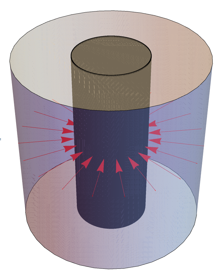
Figure 1: Pictorial representation of a GW-like perturbation in the draining bathtub geometry. The dark cylinder represents the event horizon, while pink arrows indicate the propagation direction of the GW-like perturbation.

Although this construction is described in $(2+1)$–dimensions, it can be extended to $(3+1)$–dimensions by adding an extra spatial dimension, $z$, indicating the height of the cylinder. The condition of irrotational flow implies that the $z$–component of the velocity is constant; for simplicity we assume that it vanishes. Hence in $(3+1)$–dimensions we have a vortex filament located at $r=0$ generating the metric

$$\mathrm{d}s^{2}=-c_{s}^{2}\mathrm{d}t^{2}+\left(\mathrm{d}r-\frac{A}{r}\mathrm{d}t\right)^{2}+\left(r\mathrm{d}\phi-\frac{B}{r}\mathrm{d}t\right)^{2}+\mathrm{d}z^{2}\,,$$ (58)

for the phonon excitations. This extended metric will serve as the foundation for our exploration of a system where an acoustic BH is perturbed by an analogue GW-like fluctuation that propagates radially. A schematic representation of the system is shown in Fig. 1. This choice of geometry is entirely distinct from astrophysical BHs. The background metric given by Eq.(58), with $A<0$, has indeed a cylindrical event horizon located at $r_{H}$ for all $z$. We have chosen this specific geometry for several reasons. While simpler configurations, such as a two-dimensional horizon, could be considered, the cylindrical case offers a more general approach and holds significant experimental potential. Laboratory experiments have successfully created box-like BECs Meyrath et al. (2005); Gaunt et al. (2013); Mukherjee et al. (2017), suggesting the feasibility of confining a BEC within a cylindrically symmetric trapping potential. This geometry can thus serve as a practical model for experimental analogues of gravitational phenomena. Moreover, cigar-shaped or disk-shaped BECs, which have been used in analogue gravity experimentsMuñoz de Nova et al. (2019); Hu et al. (2019), can be obtained as limiting cases of the cylindrical BEC.

IV.2 Method

We proceed to consider the various steps needed to realize a GW-like perturbation in the cylindrical geometry:

1. Cylindrical perturbations: Extend the GW-like perturbation obtained in Sec. III to the cylindrical geometry.

2. Physical requirements: Check the irrotational condition constraint, as well as the continuity and Euler equations.

3. Acoustic metric: Calculate the acoustic metric and its inverse to characterize the emergent spacetime.

4. Perturbed acoustic horizon: Investigate the position of the acoustic horizon upon interaction with the analogue GW.

As in Sec. III, it is important to distinguish between two types of fluctuations: background fluctuations, associated with metric perturbations, and the phonon fluctuations, which represent propagating modes on the emergent acoustic metric. In Appendix A, the generators of the acoustic horizon are examined to elucidate their properties under perturbations.

IV.2.1 Cylindrical perturbations

We extend the GW-like plane wave perturbation obtained in Sec. III to a cylindrical geometry. In the linear case discussed earlier, we identified the analogue of a gravitational wave by perturbing the condensate velocity along the directions perpendicular to the wave’s propagation. For the cylindrical geometry, we consider that the perturbation propagates radially, as depicted by pink arrows in Fig. 1. Consequently, the GW-like perturbation is characterized by velocity fluctuations along the angular and $z$–coordinates, denoted as $\delta v_{\phi}$ and $\delta v_{z}$, respectively. These perturbations can be obtained from those in Eq. (47) with the replacements $\delta v_{x}\to\delta v_{z}$ and $\delta v_{y}\to r/r_{0}\delta v_{\phi}$, where $r_{0}$ is a normalizing length. Due to the radial propagation direction, the term $\cos(\omega(t-z/c_{s})$ in Eq. (47) is replaced by $\cos(\omega(t-r/c_{s}))$. In conclusion, the GW-like perturbation in the cylindrical case is identified by the following velocity fluctuations:

$$\frac{\delta v_{z}}{c_{s}}= \,l(fh_{+}+gh_{\times})\cos(\omega(t-r/c_{s})),\,$$ (59)

$$\frac{\delta v_{\phi}}{c_{s}}= \frac{r_{0}}{r}b(fh_{+}+gh_{\times})\cos(\omega(t-r/c_{s})).$$ (60)

The characteristic frequencies of this system are

$$\omega_{z}=\frac{2\pi c_{s}}{L_{z}},\quad\omega_{r}=\frac{2\pi c_{s}}{L_{r}},$$ (61)

where $L_{z}$ and $L_{r}$ represent the physical dimensions of the system along the $z$ and $r$ directions, respectively. Given that the system elongates along the $z$–direction, we assume that

$$\omega_{r}>\omega_{z}\,,$$ (62)

and we consider perturbation frequencies

$$\omega\sim\omega_{z}\,,$$ (63)

thus with a wavelength of order the height of the cylinder.

IV.2.2 Physical requirements

We now check whether the irrotational condition, as well as the continuity, and Euler equations hold for the velocity perturbations in Eqs. (59) and (60). As in the Minkowskian case, we assume that the unperturbed system is homogeneous: the density, pressure and the speed of sound are taken constant. The unperturbed velocity is given by Eq. (55) with $A$ and $B$ two constants.
We begin by examining the irrotationality of the flow, checking that $\nabla\times\delta\mathbf{v}=\mathbf{0}$. We have seen that in flat spacetime the irrotational condition requires the presence of an additional velocity component; likewise here the fluctuations $\delta v_{z}$ and $\delta v_{\phi}$ satisfy the irrotational condition only if

$$\delta v_{r}= lz\omega(fh_{+}+gh_{\times})\sin(\omega(t-r/c_{s}))$$

$$+b\phi r_{0}\omega(fh_{+}+gh_{\times})\sin(\omega(t-r/c_{s}))\,,$$ (64)

which is thus the sum of two terms: one proportional to $l\,z$ and the other one to $b\,\phi$. In order to have a single-valued function we impose this second term to be zero taking $b=0$. This constraint, in turn, implies that $\delta v_{\phi}=0$, see Eq. (60). Hence, we start with a GW-like perturbation that is represented only by the velocity perturbation $\delta v_{z}$ in Eq. (59) and this induces a radial velocity perturbation

$$\frac{\delta v_{r}}{c_{s}}=lz\frac{\omega}{c_{s}}(fh_{+}+gh_{\times})\sin(\omega(t-r/c_{s})).$$ (65)

In the Minkowskian case, the velocity perturbation induced by the analogue GW was negligible (see Eq (52)), because it was of order ${\cal O}(\epsilon\omega/\omega_{x,y})$. In cylindrical geometry the induced velocity is instead ${\cal O}(\epsilon\omega/\omega_{z})$ and we cannot neglect it, see Eq .(63). Note that the radial velocity perturbation depends on the $z$ coordinate, hence it produces a time dependent bending of the acoustic horizon that changes with height. Turning to dimensionless coordinates, we express $z$ as $\tilde{z}L_{z}$ with $\bar{z}\in[0,1]$ and $r$ as $\bar{r}L_{r}$ with $\bar{r}\in[0,1]$. For convenience we choose $l=1/2\pi$ and so:

$$\frac{\delta v_{z}}{c_{s}}=\frac{1}{2\pi}(fh_{+}+gh_{\times})\cos(\omega(t-2\pi\bar{r}/\omega_{r})),$$

$$\frac{\delta v_{r}}{c_{s}}=\bar{z}\frac{\omega}{\omega_{z}}(fh_{+}+gh_{\times})\sin(\omega(t-2\pi\bar{r}/\omega_{r})).$$ (66)

In the Minkowskian case, the velocity perturbations in Eq. (47), representing the analogue GW, were solutions of the continuity and Euler equations with $\delta a=\delta n_{c}=0$. However, in the cylindrical case with an acoustic horizon, the velocity perturbations in Eq. (66) remain solutions of these equations, provided we introduce appropriate additional terms: the continuity equation forces us to take $\delta n_{c}\not=0$, and as a consequence $\delta a\not=0$. Specifically, the continuity equation holds if we include the source term

$$\delta S= \frac{2\pi}{3}n_{c}\frac{\bar{z}\bar{r}^{3}}{\bar{r}_{H}^{2}}\frac{\omega^{3}}{\omega_{r}\omega_{z}}(fh_{+}+gh_{\times})$$

$$\times\left(-1-\frac{\bar{r}_{H}}{\bar{r}}\right)\sin(\omega(t-2\pi\bar{r}/\omega_{r}))\,,$$ (67)

where

$$\bar{r}_{H}=\frac{|A|}{c_{s}L_{r}}\,,$$ (68)

is the unperturbed horizon position, see Eq. (57), in dimensionless units. Such source term induces the density fluctuation

$$\frac{\delta n_{c}}{n_{c}}= \frac{\bar{z}\bar{r}}{\bar{r}_{H}}\frac{\omega}{\omega_{z}}(fh_{+}+gh_{\times})\sin(\omega(t-2\pi\bar{r}/\omega_{r}))$$

$$+\frac{2\pi}{3}\frac{\bar{z}\bar{r}^{3}}{\bar{r}_{H}^{2}}\frac{\omega^{2}}{\omega_{r}\omega_{z}}(fh_{+}+gh_{\times})\cos(\omega(t-2\pi\bar{r}/\omega_{r})).$$ (69)

Furthermore, to maintain $c_{s}$ as the local speed of sound, we require $\delta c_{s}=0$, which leads to the introduction of a Feshbach resonance (see Eq. (10)) such that $\delta a/a=-\delta n_{c}/n_{c}$. With this choice of $\delta a$, the Euler equation holds if we include the external potential

$$\delta V_{\text{ext}}= \left(\frac{3}{8\pi}\frac{\bar{z}(\bar{r}-\bar{r}_{H})}{\bar{r}_{H}^{2}}\frac{\omega^{2}\omega_{r}}{\omega_{z}c_{s}^{2}}-\frac{\pi}{6}\frac{\bar{z}\bar{r}^{3}}{\bar{r}_{H}^{2}}\frac{\omega^{4}}{\omega_{z}\omega_{r}c_{s}^{2}}\right)\frac{\hslash^{2}}{m}$$

$$\times(fh_{+}+gh_{\times})\cos(\omega(t-2\pi\bar{r}/\omega_{r}))-\left(\bar{z}\frac{c_{s}^{2}\omega}{\omega_{z}}m\right.$$

$$\left.+\frac{1}{16\pi^{2}}\frac{\bar{z}}{\bar{r}\bar{r}_{H}}\frac{\omega\omega_{r}^{2}}{\omega_{z}c_{s}^{2}}\frac{\hslash^{2}}{m}+\frac{\bar{z}\bar{r}}{\bar{r}_{H}^{2}}\left(\frac{7}{12}\bar{r}-\frac{1}{4}\bar{r}_{H}\right)\frac{\omega^{3}}{\omega_{z}c_{s}^{2}}\frac{\hslash^{2}}{m}\right)$$

$$\times(fh_{+}+gh_{\times})\sin(\omega(t-2\pi\bar{r}/\omega_{r})).$$ (70)

In this way we obtain a physical system (irrotationality, continuity and Euler equations are satisfied), in the geometry depicted in Fig. 1, that represents an acoustic BH perturbed by an analogue GW.

IV.2.3 Acoustic metric

At this point, we compute the emergent acoustic metric tensor for phonons, given by $g_{\mu\nu}=g^{0}_{\mu\nu}+\epsilon\tilde{g}_{\mu\nu}$. For simplicity we assume vanishing tangential flow, that is we take $B=0$ in Eq. (55). Using coordinates $(c_{s}t,\bar{r},\theta,\bar{z})$, the unperturbed metric is

$$g^{0}_{\mu\nu}=\frac{n_{c}}{mc_{s}}\begin{pmatrix}-\left(1-\frac{v_{r}^{2}}{c_{s}^{2}}\right)&-\frac{v_{r}}{c_{s}}L_{r}&0&0\\ -\frac{v_{r}}{c_{s}}L_{r}&L_{r}^{2}&0&0\\ 0&0&\bar{r}^{2}L_{r}^{2}&0\\ 0&0&0&L_{z}^{2}\\ \end{pmatrix},$$ (71)

and the perturbation

$$\tilde{g}_{\mu\nu}=\frac{n_{c}}{mc_{s}}\begin{pmatrix}\tilde{g}_{00}&\tilde{g}_{01}&0&\tilde{g}_{03}\\ \tilde{g}_{01}&\tilde{g}_{11}&0&0\\ 0&0&\tilde{g}_{22}&0\\ \tilde{g}_{03}&0&0&\tilde{g}_{33}\\ \end{pmatrix},$$ (72)

has components

$$\tilde{g}_{00}=-\left(1-\frac{v_{r}^{2}}{c_{s}^{2}}\right)\frac{\delta n_{c}}{n_{c}}+2\frac{v_{r}\delta v_{r}}{c_{s}^{2}},$$ (73)

$$\tilde{g}_{01}=L_{r}\left(-\frac{\delta v_{r}}{c_{s}}-\frac{v_{r}}{c_{s}}\frac{\delta n_{c}}{n_{c}}\right),$$ (74)

$$\tilde{g}_{03}=-\frac{\delta v_{z}}{c_{s}}L_{z}\,,\quad\tilde{g}_{11}=\frac{\delta n_{c}}{n_{c}}L_{r}^{2},$$ (75)

$$\tilde{g}_{22}=\tilde{r}^{2}L_{r}^{2}\frac{\delta n_{c}}{n_{c}}\,,\quad\tilde{g}_{33}=\frac{\delta n_{c}}{n_{c}}L_{z}^{2}\,,$$ (76)

that are the fluctuations of the metric induced by the GW analogue. Far from the horizon, these perturbations can be seen as fluctuations around the Minkowski metric. Near the horizon, they represent a perturbation of the cylindrical acoustic metric. Next, we compute the inverse of the metric defined by the relation $g_{\mu\nu}g^{\nu\alpha}=\delta_{\mu}{}^{\alpha}$, and we write it as

$$g^{\mu\nu}=g^{\mu\nu}_{0}-\epsilon\tilde{g}^{\mu\nu}.$$ (77)

In the coordinates $(c_{s}t,\tilde{r},\theta,\tilde{z})$, the unperturbed inverse metric is

$$g^{\mu\nu}_{0}=\frac{c_{s}m}{n_{c}}\begin{pmatrix}-1&-\frac{v_{r}}{c_{s}L_{r}}&0&0\\ -\frac{v_{r}}{c_{s}L_{r}}&\frac{1}{L_{r}^{2}}\left(1-\frac{v_{r}^{2}}{c_{s}^{2}}\right)&0&0\\ 0&0&\frac{1}{\tilde{r}^{2}L_{r}^{2}}&0\\ 0&0&0&\frac{1}{L_{z}^{2}}\\ \end{pmatrix},$$ (78)

and the inverse perturbation is

$$\tilde{g}^{\mu\nu}=\frac{mc_{s}}{n_{c}}\begin{pmatrix}\tilde{g}^{00}&\tilde{g}^{01}&0&\tilde{g}^{03}\\ \tilde{g}^{01}&\tilde{g}^{11}&0&\tilde{g}^{13}\\ 0&0&\tilde{g}^{22}&0\\ \tilde{g}^{03}&\tilde{g}^{13}&0&\tilde{g}^{33}\end{pmatrix},$$ (79)

with components

$$\tilde{g}^{00}=-\frac{\delta n_{c}}{n_{c}},$$ (80)

$$\tilde{g}^{01}=\left(-\frac{\delta n_{c}}{n_{c}}\frac{v_{r}}{c_{s}}+\frac{\delta v_{r}}{c_{s}}\right)\frac{1}{L_{r}},$$ (81)

$$\tilde{g}^{03}=\frac{\delta v_{z}}{c_{s}}\frac{1}{L_{z}},$$ (82)

$$\tilde{g}^{11}=\left(2\frac{v_{r}\delta v_{r}}{c_{s}^{2}}+\frac{\delta n_{c}}{n_{c}}-\frac{v_{r}^{2}}{c_{s}^{2}}\frac{\delta n_{c}}{n_{c}}\right)\frac{1}{L_{r}^{2}},$$ (83)

$$\tilde{g}^{13}=\frac{v_{r}\delta v_{z}}{c_{s}^{2}}\frac{1}{L_{r}L_{z}},$$ (84)

$$\tilde{g}^{22}=\frac{1}{\tilde{r}^{2}L_{r}^{2}}\frac{\delta n_{c}}{n_{c}},$$ (85)

$$\tilde{g}^{33}=\frac{\delta n_{c}}{n_{c}}\frac{1}{L_{z}^{2}}.$$ (86)

From the inverse metric we can determine the event horizon’s characteristics and generators.

IV.2.4 Perturbed acoustic horizon

We now determine the displacement of the horizon position determined by the impinging GW analogue. In general, the horizon position is given by the condition $|v_{r}|_{r_{H}}=c_{s}$. In the unperturbed system, the horizon is located in $\bar{r}_{H}$ given in Eq. (68). The GW analogue propagation is determined by the velocity fluctuation $\delta v_{r}$ in Eq. (65). Consequently, the acoustic horizon is displaced at $\tilde{r}_{H}^{\text{new}}=\tilde{r}_{H}+\epsilon\delta\tilde{r}_{H}$, which satisfies:

$$|v_{r}+\epsilon\delta v_{r}|_{\tilde{r}_{H}^{\text{new}}}=c_{s}.$$ (87)

Solving Eq. (87), we find the horizon’s displacement is

$$\frac{\delta\tilde{r}_{H}}{\tilde{r}_{H}}=-\tilde{z}\frac{\omega}{\omega_{z}}(fh_{+}+gh_{\times})\sin(\omega(t-2\pi\tilde{r}_{H}/\omega_{r}))\,,$$ (88)

indicating that it is opposite to the sign of the radial velocity fluctuation, see Eq. (66), while the fluctuation $\delta v_{z}$ has no effect on the horizon’s position. The horizon’s displacement vanishes at $\tilde{z}=0$ and for $\tilde{z}\neq 0$ it depends on the sign of $\sin(\omega(t-2\pi\tilde{r}_{H}/\omega_{r}))$. At a given time $t$, such that $\sin(\omega(t-2\pi\tilde{r}_{H}/\omega_{r}))>0$, we have that $\delta\tilde{r}_{H}<0$ and the displacement decreases as $\tilde{z}$ increases, see Fig.  2.

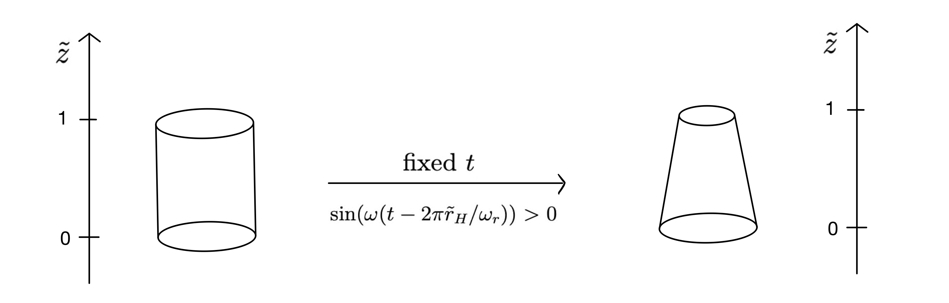
Figure 2: Schematic representation of the perturbation of the acoustic horizon. Left: unperturbed horizon. Right: perturbed acoustic horizon at a fixed time such that $\sin(\omega(t-2\pi\tilde{r}_{H}/\omega_{r}))>0$. The size of the perturbation is enhanced for clarity.

At time $t$ such that $\sin(\omega(t-2\pi\tilde{r}_{H}/\omega_{r}))<0$, we have he opposite behavior: $\delta\tilde{r}_{H}$ increases linearly with $\tilde{z}$, see Fig. 3.

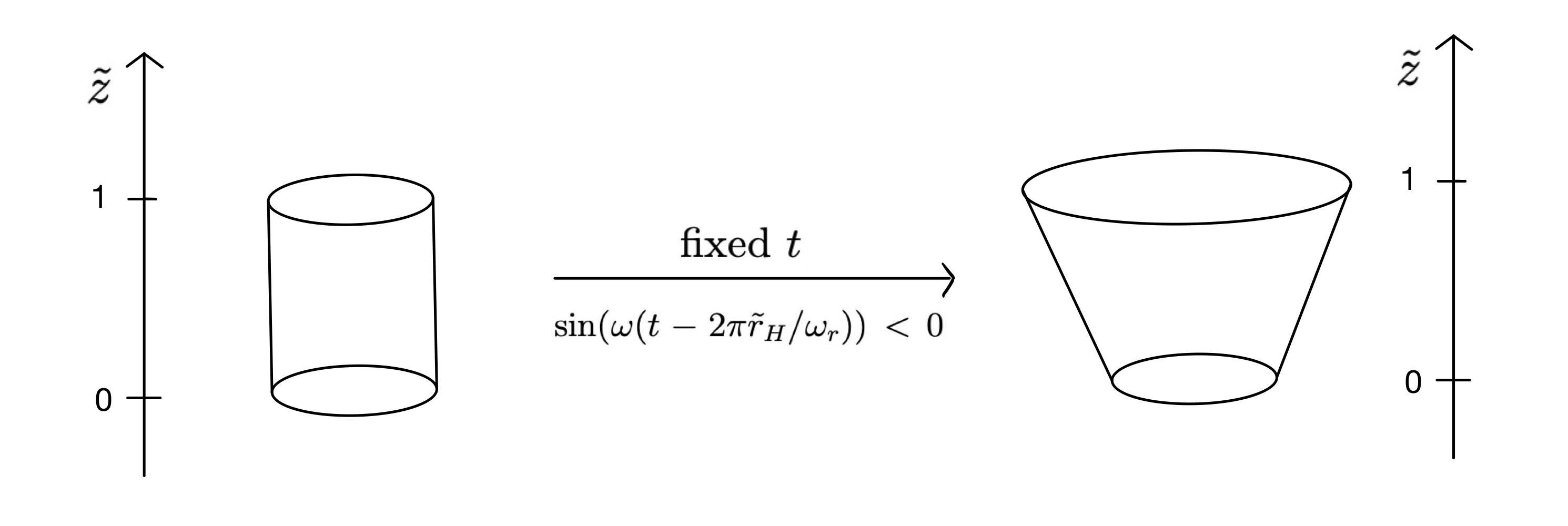
Figure 3: Schematic representation of the perturbation of the acoustic horizon. Left: unperturbed horizon. Right: perturbed acoustic horizon at a fixed time such that $\sin(\omega(t-2\pi\tilde{r}_{H}/\omega_{r}))<0$. The size of the perturbation is enhanced for clarity.

If we now examine the scenario at fixed $\tilde{z}\neq 0$, and we observe the changes over time, we find that the horizon displacement fluctuates around zero as shown in Fig. 4: the event horizon expands or contracts due to the GW analogue propagation. The magnitude of the dilatation depends on the considered height: it vanishes for $\bar{z}=0$ and it is maximal for $\bar{z}=1$.

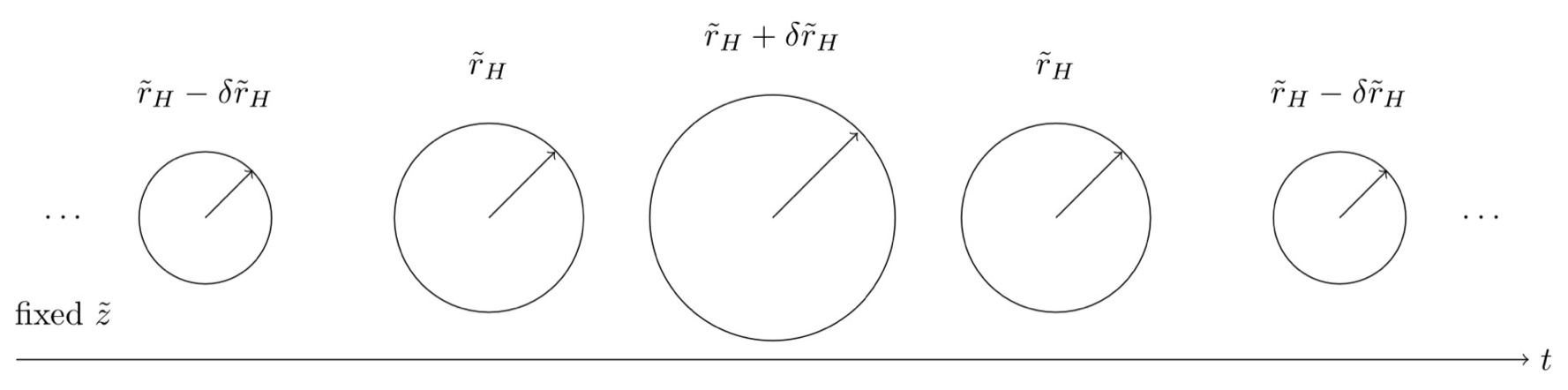
Figure 4: Schematic representation of the perturbation of the perturbed acoustic horizon in the $\tilde{x}\tilde{y}$ plane. At fixed $\tilde{z}>0$ the horizon is a circle that oscillates as time lapses.

Differently from the flat spacetime case where GWs do not cause phonon production, when GWs impinge onto an acoustic horizon they induce on it periodic deformations which turns into a stimulated amplification of the Hawking phonon radiation in a phenomenon resembling the dynamical Casimir effect Sabin, Bruschi, and Fuentes (2014). This process was described in details in Luisa Chiofalo et al., 2024 in the case of a planar acoustic horizon under the action of a small velocity shear in background flow. Something similar takes place for the system considered here with a cylindrical geometry and the shear perturbation being originated by the impinging GWs. The expansion or contraction observed at a fixed $\tilde{z}$ corresponds to an oscillation of the tilting of the horizon. Due to this tilt, the radiated phonons, which are predominantly emitted in the direction perpendicular to the horizon, experience a change in their propagation direction as compared to the unperturbed caseShapiro and Teukolsky (1983); Mannarelli et al. (2021). Focusing for instance on the $\tilde{x}\tilde{z}$ plane at $\tilde{y}=0$ and considering only the half-plane $\tilde{x}>0$, the situation closely resembles the analysis conducted in Sec. V of Ref. Luisa Chiofalo et al., 2024, where the shear viscosity to entropy density ratio $\eta/s$ at the acoustic horizon was calculated to be equal to $1/4\pi$, namely, the KSS lower bound Kovtun, Son, and Starinets (2005). Although a planar horizon was considered in Ref. Luisa Chiofalo et al., 2024, that result holds here as well: in both cases the relevant effect is that given by the bending of the horizon surface with respect to the $\tilde{z}$ axis.

V Conclusions and future perspectives

Developing a system that enables an in-depth investigation of acoustic horizons through perturbations is crucial for addressing fundamental theoretical questions regarding the physics of BHs. In this paper, we have designed a perturbation that closely mimics a classical GW and applied it to excite an acoustic horizon. We first demonstrate that it is possible to configure a BEC such that the metric perturbation experienced by phonons resembles that of a GW in Minkowski space in a specific gauge. Subsequently, we considered the effect of this perturbation, adapted to the new symmetry of the system, on an acoustic cylindrical BH. With the proposed approach we have established a laboratory-reproducible system where to study how an acoustic horizon responds to perturbations closely modeled after GWs. In particular, experiments with ultra-cold atoms can be designed to replicate these systems in order to test the theoretical predictions arising from this research. These models open avenues for diverse future studies.

Firstly, the shear viscosity to entropy density ratio ($\eta/s$) of the acoustic horizon can be assessed. One approach is to determine and compare its value with that of a real BH in general relativity Chirco and Liberati (2010). Additionally, it is important to check whether this ratio adheres the universal lower bound of $\eta/s$, proposed in the AdS/CFT contextKovtun, Son, and Starinets (2005). This bound is conjectured to be $1/4\pi$ for any fluid in nature Cremonini (2011); Kovtun, Son, and Starinets (2003). However, the conditions under which this bound can be saturated by a matter system, given the known symmetries, remain an open question Adams et al. (2012). Thus, investigating $\eta/s$ for acoustic black holes could be crucial to determine if it saturates this bound and to establish whether the ratio for acoustic black holes is universal or dependent on specific hydrodynamic conditions.

Additionally, the surface reflectivity of the acoustic horizon can be explored and related to the membrane fluid viscosity Oshita, Wang, and Afshordi (2020).
Moreover, the analogue GW perturbation discussed in this paper can be analyzed in greater details. A particularly intriguing aspect is how, despite the absence of spin–2 modes in the system, we can still replicate a spin–2 perturbation of the metric. It might be worthwhile to study the quantization of this classical analogue GW to investigate whether its quanta can be identified and to predict the equation of motion for this mode. Although quasi-normal modes of acoustic black holes have been studied previously Berti, Cardoso, and Lemos (2004), examining this spin–2 perturbation could potentially provide a new avenue for approximating a spin–2 test field analysis Toshmatov et al. (2015). Furthermore, we can explore gravitational memory in these systems to understand how the emergent spacetime responds when an analogue GW passes through it, and whether there are any symmetries of the system related to itFavata (2010).

The authors have no conflicts to disclose.

Appendix A Horizon’s generators

To characterize the kinematics of the horizon, we compute the null vector field that is simultaneously tangent and orthogonal to the null congruence of the geodesics generating the horizon. The vector field normal to the hypersurface $S=\text{constant}$ has the general expression

$$k^{\mu}=\ell(x)g^{\mu\nu}\partial_{\nu}S\,,$$ (89)

with $\ell(x)$ an arbitrary non-vanishing function of the coordinates. Hereafter we take for simplicity $\ell(x)=1$.
We first compute $k^{\mu}$ in the unperturbed system. We consider the family of hypersurfaces

$$S=\tilde{r}-\tilde{r}_{H}=\text{constant}\,,$$ (90)

where $\bar{r}_{H}$ is given in Eq. (68); the acoustic horizon corresponds to $S=0$. For the considered hypersurface

$$\partial_{\nu}S=(0,1,0,0)\,,$$ (91)

hence, using the inverse of the metric in Eq. (78), we obtain that the vector normal to the hypersurface $S$ is given by

$$k^{\mu}=\left(\frac{m}{2\pi n_{c}}\omega_{r}\frac{\tilde{r}_{H}}{\tilde{r}},\frac{m}{4\pi^{2}n_{c}c_{s}}\omega_{r}^{2}\left(1-\frac{\tilde{r}_{H}^{2}}{\tilde{r}^{2}}\right),0,0\right),$$ (92)

and then

$$g^{0}_{\mu\nu}k^{\mu}k^{\nu}=\frac{m}{4\pi^{2}n_{c}c_{s}}\omega_{r}^{2}\left(1-\frac{\tilde{r}_{H}^{2}}{\tilde{r}^{2}}\right).$$ (93)

Since at the horizon $v_{r}^{2}=c_{s}^{2}$, we find that

$$\left.g^{0}_{\mu\nu}k^{\mu}k^{\nu}\right|_{S=0}=0\,,$$ (94)

meaning that the acoustic horizon is a null hypersurface.
For the computation of the null vector field in the system perturbed by the GW analogue, we have to consider that the inverse of the metric is given by Eq. (77) and that the position of the acoustic horizon is shifted to $\tilde{r}_{H}+\epsilon\delta\tilde{r}_{H}$, where $\delta\tilde{r}_{H}$ is in Eq. (88). For these reasons we define a new family of hypersurfaces:

$$S_{\text{new}}=\tilde{r}-\left(\tilde{r}_{H}+\epsilon\delta\tilde{r}_{H}\right)=\text{constant}\,,$$ (95)

and the acoustic horizon hypersurface is $S_{\text{new}}=0$. In this case

$$\partial_{\nu}S_{\text{new}}=(0,1,0,0)-\epsilon\partial_{\nu}\delta\tilde{r}_{H}\,,$$ (96)

thus the components of the normal vector field, that we now call $k_{\text{new}}^{\mu}$, at the leading order in the perturbations are given by

$$k_{\text{new}}^{\mu}=g_{0}^{\mu\nu}\partial_{\nu}S-\epsilon\tilde{g}^{\mu\nu}\partial_{\nu}S-\epsilon g_{0}^{\mu\nu}\partial_{\nu}\delta\tilde{r}_{H}\,.$$ (97)

Therefore, $k_{\text{new}}^{\mu}$ is identical to that of the unperturbed system at zeroth order in $\epsilon$, see Eq. (92), with corrections at order $\epsilon$ arising from both metric perturbations and changes in the horizon’s position. Its components are given by

$$k_{\text{new}}^{0} =k^{0}+\epsilon(fh_{+}+gh_{\times})\left[\frac{m}{n_{c}}\frac{\tilde{z}}{\pi}\frac{\omega\omega_{r}}{\omega_{z}}\sin(\omega T_{\text{eff}})\right.$$ (98)

$$\left.-\left(\frac{1}{3}\frac{m}{n_{c}}\frac{\omega^{2}}{\omega_{z}}\frac{\tilde{r}^{2}\tilde{z}}{\tilde{r}_{H}}+\frac{m}{n_{c}}\tilde{z}\tilde{r}_{H}\frac{\omega^{2}}{\omega_{z}}\right)\cos(\omega T_{\text{eff}})\right],$$

$$k_{\text{new}}^{1} =k^{1}+\epsilon(fh_{+}+gh_{\times})\left[\left(\frac{m}{2\pi n_{c}c_{s}}\frac{\omega^{2}\omega_{r}}{\omega_{z}}\frac{\tilde{z}\tilde{r}_{H}^{2}}{\tilde{r}}\right.\right.$$ (99)

$$\left.+\frac{m}{6\pi n_{c}c_{s}}\frac{\omega^{2}\omega_{r}}{\omega_{z}}\frac{\tilde{z}\tilde{r}}{\tilde{r}_{H}^{2}}(-\tilde{r}^{2}+\tilde{r}_{H}^{2})\right)\cos(\omega T_{\text{eff}})$$

$$\left.-\frac{m}{4\pi^{2}n_{c}c_{s}}\frac{\omega\omega_{r}^{2}}{\omega_{z}}\frac{\tilde{z}}{\tilde{r}\tilde{r}_{H}}(\tilde{r}^{2}-3\tilde{r}_{H}^{2})\sin(\omega T_{\text{eff}})\right],$$

$$k_{\text{new}}^{2}=0,$$ (100)

$$k_{\text{new}}^{3} =\epsilon(fh_{+}+gh_{\times})\left(\frac{m}{4\pi^{2}n_{c}c_{s}}\omega\omega_{z}\tilde{r}_{H}\sin(\omega T_{\text{eff}})\right.$$ (101)

$$\left.+\frac{m}{8\pi^{3}n_{c}c_{s}}\omega_{z}\omega_{r}\frac{\tilde{r}_{H}}{\tilde{r}}\cos(\omega T_{\text{eff}})\right),$$

where for simplicity we have defined $T_{\text{eff}}=t-2\pi\tilde{r}/\omega_{r}$. Now, we compute $g_{\mu\nu}k_{\text{new}}^{\nu}k_{\text{new}}^{\mu}$ at the acoustic horizon, so at $S_{\text{new}}=0$, and we call it $K$. We find:

$$K=\epsilon 4\pi\frac{n_{c}c_{s}}{m}\frac{\omega^{2}}{\omega_{r}\omega_{z}}\tilde{r}_{H}\tilde{z}(fh_{+}+gh_{\times})\cos(\omega T_{\text{eff}}).$$ (102)

Unlike the unperturbed case, where $g_{\mu\nu}k^{\mu}k^{\nu}$ at the acoustic horizon is equal to 0 (see Eq. (94)), here we have a dynamical horizon and because of that, it is not required to be a null hypersurface Ashtekar and Krishnan (2003). Depending on the sign of the cosine we can have a null, timelike or spacelike hypersurface. However, for a Killing horizon this quantity should be zero and indeed for sufficiently low fluctuations this term vanishes: it is of order $\mathcal{O}(\epsilon\omega^{2}/\omega_{r}\omega_{z})$. The null vector field computed in this appendix allows to evaluate the expansion rate, shear, and rotation of the null geodesic congruence Poisson (2004). We will discuss this topic in a future publication.

References

- LIGO Scientific Collaboration and Virgo Collaboration (2016) LIGO Scientific Collaboration and Virgo Collaboration, “Observation of Gravitational Waves from a Binary Black Hole Merger,” Phys. Rev. Lett. 116, 061102 (2016), arXiv:1602.03837 .
- Fu et al. (2024) G. Fu, Y. Liu, B. Wang, J.-P. Wu, and C. Zhang, “Probing Quantum Gravity Effects with Eccentric Extreme Mass-Ratio Inspirals,” arXiv e-prints , arXiv:2409.08138 (2024), arXiv:2409.08138 .
- Steinhauer (2016) J. Steinhauer, “Observation of quantum Hawking radiation and its entanglement in an analogue black hole,” Nature Physics 12, 959–965 (2016), arXiv:1510.00621 .
- Unruh (1981) W. G. Unruh, “Experimental black-hole evaporation?” Physical Review Letters 46, 1351–1353 (1981).
- Mannarelli et al. (2021) M. Mannarelli, D. Grasso, S. Trabucco, and M. L. Chiofalo, “Hawking temperature and phonon emission in acoustic holes,” Physical Review D 103, 076001 (2021).
- Hartley et al. (2018) D. Hartley, T. Bravo, D. Rätzel, R. Howl, and I. Fuentes, “Analogue simulation of gravitational waves in a -dimensional bose-einstein condensate,” Physical Review D 98, 025011 (2018).
- Barceló, Liberati, and Visser (2005) C. Barceló, S. Liberati, and M. Visser, “Analogue Gravity,” Living Reviews in Relativity 8, 12 (2005), arXiv:gr-qc/0505065 .
- Dalfovo et al. (1999) F. Dalfovo, S. Giorgini, L. P. Pitaevskii, and S. Stringari, “Theory of Bose-Einstein condensation in trapped gases,” Rev. Mod. Phys. 71, 463–512 (1999), arXiv:cond-mat/9806038 .
- Maggiore (2007) M. Maggiore, Gravitational Waves. Vol. 1: Theory and Experiments (Oxford University Press, 2007).
- Chin et al. (2010) C. Chin, R. Grimm, P. Julienne, and E. Tiesinga, “Feshbach resonances in ultracold gases,” Review of Modern Physics 82, 1225–1286 (2010).
- Coviello (2024) C. Coviello, “Gravitational waves and black hole perturbations in acoustic analogues,” arXiv e-prints (2024), arXiv:2409.15403 .
- Schützhold (2018) R. Schützhold, “Interaction of a bose-einstein condensate with a gravitational wave,” Phys. Rev. D 98, 105019 (2018), arXiv:1807.07046 .
- Visser (1998) M. Visser, “Acoustic black holes: horizons, ergospheres and hawking radiation,” Classical and Quantum Gravity 15, 1767 (1998).
- Meyrath et al. (2005) T. P. Meyrath, F. Schreck, J. L. Hanssen, C. S. Chuu, and M. G. Raizen, “Bose-Einstein condensate in a box,” Physical Review A 71, 041604 (2005), arXiv:cond-mat/0503590 .
- Gaunt et al. (2013) A. L. Gaunt, T. F. Schmidutz, I. Gotlibovych, R. P. Smith, and Z. Hadzibabic, “Bose-Einstein Condensation of Atoms in a Uniform Potential,” Physical Review Letters 110, 200406 (2013), arXiv:1212.4453 .
- Mukherjee et al. (2017) B. Mukherjee, Z. Yan, P. B. Patel, Z. Hadzibabic, T. Yefsah, J. Struck, and M. W. Zwierlein, “Homogeneous atomic fermi gases,” Physical Review Letters 118, 123401 (2017).
- Muñoz de Nova et al. (2019) J. R. Muñoz de Nova, K. Golubkov, V. I. Kolobov, and J. Steinhauer, “Observation of thermal Hawking radiation and its temperature in an analogue black hole,” Nature 569, 688–691 (2019), arXiv:1809.00913 .
- Hu et al. (2019) J. Hu, L. Feng, Z. Zhang, and C. Chin, “Quantum simulation of Unruh radiation,” Nature Physics 15, 785–789 (2019).
- Sabin, Bruschi, and Fuentes (2014) C. Sabin, M. Bruschi, David Edward Ahmadi, and I. Fuentes, “Phonon creation by gravitational waves,” New J. Phys. 16, 085003 (2014), arXiv:1402.7009 .
- Luisa Chiofalo et al. (2024) M. Luisa Chiofalo, D. Grasso, M. Mannarelli, and S. Trabucco, “Dissipative processes at the acoustic horizon,” New J. Phys. 26, 053021 (2024), arXiv:2202.13790 .
- Shapiro and Teukolsky (1983) S. L. Shapiro and S. A. Teukolsky, Black holes, white dwarfs and neutron stars. The physics of compact objects (Wiley-VCH, 1983).
- Mannarelli et al. (2021) M. Mannarelli, D. Grasso, S. Trabucco, and M. L. Chiofalo, “Phonon emission by acoustic black holes,” arXiv e-prints , arXiv:2109.11831 (2021), arXiv:2109.11831 .
- Kovtun, Son, and Starinets (2005) P. Kovtun, D. T. Son, and A. O. Starinets, “Viscosity in strongly interacting quantum field theories from black hole physics,” Phys. Rev. Lett. 94, 111601 (2005), arXiv:hep-th/0405231 .
- Chirco and Liberati (2010) G. Chirco and S. Liberati, “Nonequilibrium thermodynamics of spacetime: The role of gravitational dissipation,” Physical Review D 81, 024016 (2010).
- Cremonini (2011) S. Cremonini, “The Shear Viscosity to Entropy Ratio: a Status Report,” Modern Physics Letters B 25, 1867–1888 (2011), arXiv:1108.0677 .
- Kovtun, Son, and Starinets (2003) P. Kovtun, D. T. Son, and A. O. Starinets, “Holography and hydrodynamics: diffusion on stretched horizons,” Journal of High Energy Physics 2003, 064 (2003).
- Adams et al. (2012) A. Adams, L. D. Carr, T. Schäfer, P. Steinberg, and J. E. Thomas, “Strongly correlated quantum fluids: ultracold quantum gases, quantum chromodynamic plasmas and holographic duality,” New Journal of Physics 14, 115009 (2012), arXiv:1205.5180 .
- Oshita, Wang, and Afshordi (2020) N. Oshita, Q. Wang, and N. Afshordi, “On reflectivity of quantum black hole horizons,” Journal of Cosmology and Astroparticle Physics 2020, 016 (2020), arXiv:1905.00464 .
- Berti, Cardoso, and Lemos (2004) E. Berti, V. Cardoso, and J. P. Lemos, “Quasinormal modes and classical wave propagation in analogue black holes,” Phys. Rev. D 70, 124006 (2004), arXiv:gr-qc/0408099 .
- Toshmatov et al. (2015) B. Toshmatov, A. Abdujabbarov, Z. Stuchlík, and B. Ahmedov, “Quasinormal modes of test fields around regular black holes,” Physical Review D 91 (2015), 10.1103/PhysRevD.91.083008, arXiv:1503.05737 .
- Favata (2010) M. Favata, “The gravitational-wave memory effect,” Classical and Quantum Gravity 27, 084036 (2010), arXiv:1003.3486 .
- Ashtekar and Krishnan (2003) A. Ashtekar and B. Krishnan, “Dynamical horizons and their properties,” Physical Review D 68, 104030 (2003), arXiv:gr-qc/0308033 .
- Poisson (2004) E. Poisson, A relativist’s toolkit : the mathematics of black-hole mechanics (Cambridge University Press, 2004).