Learning to Ground Existentially Quantified Goals

Abstract

Goal instructions for autonomous AI agents cannot assume that objects have unique names. Instead, objects in goals must be referred to by providing suitable descriptions. However, this raises problems in both classical planning and generalized planning. The standard approach to handling existentially quantified goals in classical planning involves compiling them into a DNF formula that encodes all possible variable bindings and adding dummy actions to map each DNF term into the new, dummy goal. This preprocessing is exponential in the number of variables. In generalized planning, the problem is different: even if general policies can deal with any initial situation and goal, executing a general policy requires the goal to be grounded to define a value for the policy features. The problem of grounding goals, namely finding the objects to bind the goal variables, is subtle: it is a generalization of classical planning, which is a special case when there are no goal variables to bind, and constraint reasoning, which is a special case when there are no actions. In this work, we address the goal grounding problem with a novel supervised learning approach. A GNN architecture, trained to predict the cost of partially quantified goals over small domain instances is tested on larger instances involving more objects and different quantified goals. The proposed architecture is evaluated experimentally over several planning domains where generalization is tested along several dimensions including the number of goal variables and objects that can bind such variables. The scope of the approach is also discussed in light of the known relationship between GNNs and $C_{2}$ logics.

1 Introduction

In classical planning, the usual assumption is that objects have unique names, and goals are described using these names. For instance, a goal might be to place block A on top of block B, where A and B are specific blocks. A similar assumption is made in generalized planning, where a policy is sought to handle reactively any instances within a given domain. To apply the general plan to a particular domain instance, it is assumed that the goal consists of a conjunction of grounded atoms, with objects referred to by unique names.

However, instructions for goals in autonomous AI agents cannot assume that objects have individual, known names. Instead, goals must be expressed by referring to objects using suitable descriptions. For instance, the instruction to place the large, yellow ball next to the blue package or to construct a tower of 6 blocks, alternating between blue and red blocks, does not specify the objects uniquely, and it’s indeed part of the problem to select the right objects.

To address goals in classical planning that do not include unique object names, existentially quantified goals are used (?; ?; ?). For example, the goal of placing the large, yellow ball next to the blue package can be expressed with the following formula:

$$\exists x,y:\big{[} \textsc{Ball}(x)\wedge\textsc{Large}(x)\wedge\textsc{Yellow}(x)$$

$$\wedge\textsc{Package}(y)\wedge\textsc{Blue}(y)\wedge\textsc{Next}(x,y)\big{]}.$$

However, there are not many classical planners that support existentially quantified goals because dealing with such goals is computationally hard, even when actions are absent. Determining whether an existentially quantified goal is true in a state is indeed NP-hard, as these goals can easily express constraint satisfaction problems (?). For example, consider a graph coloring problem over a graph $G=\langle V,E\rangle$, where $V$ represents vertices $i\in V$ and $E$ represents edges $(k,j)\in E$. This problem can be expressed via the goal:

$$\exists x_{1},\ldots,x_{n}:\Bigg{[}\bigwedge_{i\in V}\textsc{Color}(i,x_{i})\Bigg{]}\wedge\Bigg{[}\bigwedge_{(k,j)\in E}\textsc{Neq}(x_{k},x_{j})\Bigg{]}.$$

This expression applies to an initial state with ground atoms $\textsc{Color}(i,x)$, where $x$ is a possible color of vertex $i$, and ground atoms $\textsc{Neq}(x,x^{\prime})$ express that $x$ and $x^{\prime}$ are distinct.

The standard approach to handling existentially quantified goals in classical planning involves eliminating them by transforming them into a grounded DNF formula that encodes all possible variable bindings. This process also involves adding dummy actions for each DNF term to map them to a new, dummy goal (?). However, this preprocessing step is exponential in the number of variables. For instance, in the graph coloring example, it results in several terms and dummy actions that grow exponentially with the number of vertices $n$.

The problem of grounding goals, which involves finding objects to bind the goal variables, is subtle. It is a generalization of standard classical planning where there are no goal variables to bind, and it is a special case of constraint reasoning, which is computationally hard even without considering actions. Conceptually, the interesting problems lie between these two extremes, in the presence of multiple possible bindings for the goal variables, each resulting in a fully grounded goal with a ”cost” determined by the number of steps needed to reach it from the initial state. Optimal bindings, or groundings, replace the goal variables with constants to achieve grounded goals with minimum cost. In action-less problems representing constraint satisfaction problems, the cost of the bindings (i.e., the cost of the resulting grounded goals) is either zero or infinity. In planning problems with existentially quantified goals, the cost of the possible groundings depends on the initial state, the actions, and the structure of the goal, and can be any natural number or infinity. For example, in the planning problem with the initial and goal states shown in Figures 1(a) and 1(b) below, the optimal grounding binds the two bottom blocks in the goal to F and A, so that the first move places A on F.

In this work, we tackle the problem of grounding goals as a generalized planning problem (?; ?; ?). Here, both the training and test instances are assumed to contain partially quantified goals; that is, a combination of grounded and existentially quantified variables. We use a graph neural network (GNN) architecture, trained using supervised learning to predict the cost $V(P)$ of partially quantified goals over small domain instances $P$ and test it on larger instances $P^{\prime}$ involving more objects and different goals. The bindings of the goal variables are then obtained sequentially by greedily grounding one variable at a time, without any search, neither in the problem state space nor the space of goal bindings. Once the variables in the goal of an instance $P$ have been grounded, existing methods can be used to obtain a plan for the fully grounded problem $P^{\prime}$, using standard classical or generalized planners that expect grounded goals.

The paper is organized as follows: we start by explaining the learning task through an example, and then review classical planning, generalized planning, and existentially quantified goals. Next, we describe the task, introduce our proposed learning method, present the experimental results and detailed analysis over an example.

2 Example: Visit-1

We begin with an example to illustrate our learning task, estimating the cost of existentially quantified goals in planning, and why GNNs provide a handle on this problem given the known correspondence between GNNs and $C_{2}$, the fragment of first-order logic with two variables and counting (?; ?). Indeed, we show that the general value (cost) function for the problem can be expressed in $C_{2}$ and hence can be learned with GNNs.

The example is a variation of the Visitall domain where a robot is placed on a grid and can move up, down, left, or right. In the original domain, the goal is for the robot to visit all the cells in the grid. Each cell is represented as a single object, and two cells $x$ and $y$ are considered adjacent if there is a $\textsc{Connected}(x,y)$ atom in the state. A cell $x$ is marked as visited with a $\textsc{Visited}(x)$ atom. The location of the robot is given by $\textsc{At-Robot}(x)$, where $x$ is a cell.

In our variation, cells have colors from a fixed set of colors $\mathcal{C}$ and the goal is to visit a cell of a given color. The cost of the problem is thus given by the distance to the closest cell of that color. For reasons to be elaborated later, the distances involved must be bounded with the set $\mathcal{D}$ representing the distances up to such a bound. The goals have the form:

$$G=\exists x:\textsc{C}(x)\wedge\textsc{Visited}(x),$$

where C is any of the colors in $\mathcal{C}$. Later on, we will consider a further variation of the problem where cells of different colors are to be visited. The objective is to express the cost function for this family of problems using Boolean features definable in $C_{2}$ so that the cost function can be learned with GNNs.

The Boolean function $\text{SP}_{d,\textsc{C}}(x)$ determines the existence of a shortest path of length $d$ from $x$ to a cell with color C:

$$\text{P}_{0,\textsc{C}}(x) =\textsc{C}(x)$$

$$\text{P}_{d,\textsc{C}}(x) =\exists y:\textsc{Connected}(x,y)\wedge\text{P}_{d-1,\textsc{C}}(y)$$

$$\text{SP}_{d,\textsc{C}}(x) =\text{P}_{d,\textsc{C}}(x)\wedge\neg\text{P}_{d-1,\textsc{C}}(x)$$

If we let $N$ stand for the max distance plus 1, the value function $V^{*}$ can then be expressed as:

$$\textsc{G}_{\textsc{C}} =\exists v:\textsc{C}_{G}(v)$$

$$D_{d,\textsc{C}} =\textsc{G}_{\textsc{C}}\wedge\exists x:\left[\textsc{At-Robot}(x)\wedge\text{SP}_{d,\textsc{C}}(x)\right]$$

$$V^{*}(s;G) =\min_{d\in\mathcal{D},\textsc{C}\in\mathcal{C}}d\cdot[\![D_{d,\textsc{C}}]\!]+N\cdot[\![\neg D_{d,\textsc{C}}]\!]$$

Here, $s$ represents a state, and $G$ denotes a goal. The notation $[\![\cdot]\!]$ is the Iverson bracket, and $\textsc{C}_{G}$ refers to the colors specified in $G$. When predicate names are used without subscripts, they refer to $s$. If we assume that the state $s$ does not contain any Visited atoms, then $V^{*}$ calculates the distance to the nearest cell with the color C, provided such a cell exists. If no such cell exists, the value is set to $N$.

We will learn $V^{*}$ using GNNs. Since the expressiveness of GNNs is limited by two-variable first-order logic $C_{2}$, if $V^{*}$ cannot be expressed with $C_{2}$ features, it will not be learnable by GNNs. Existentially quantified goals are thus handled “by free” by GNNs as long as they do not get out of these limits. Moreover, existentially quantified goals with more than two variables are not necessarily a problem if they are equivalent to formulas in $C_{2}$. For example, the goal of building a tower of five blocks is naturally written in terms of five variables, yet the formula is equivalent to a formula with two variables only that are quantified multiple times.

3 Related work

Quantification in planning. Since the middle nineties, planners usually ground all actions and goals to improve efficiency. This does not rule out the use of existential and universal quantification in action preconditions and effects, and goals (?; ?). Universal quantification can be replaced by conjunctions, while existential quantification by disjunctions (?). The problem with existential quantification in the goal is that the number of resulting disjuncts is exponential in the number of goal variables. In action preconditions, the problem is less critical as the number of variables is bounded by the arity of the action schemas.

Lifted planning. Modern, lifted planners aim to approximate the performance of fully grounded planners without having to ground actions or goals (?; ?). The problem with non-grounded goals is that they do not result in equally informed heuristics, and approaches that aim to compute informed heuristics without grounding the actions or goals carry a significant overhead (?).

Generalized planning. The problem of learning policies for solving collections of problems involving different number of objects and goals have been approached with symbolic (?; ?; ?; ?; ?; ?) and deep learning methods (?; ?; ?; ?; ?), yet in practically all cases, goals are assumed to be fully grounded.

Grounding instructions in RL. In reinforcement learning, the problem of grounding instructions is the problem of understanding and carrying out the given instructions (?; ?; ?). The key difference with generalized planning is that the structure of the states and goals, both sets of ground atoms over a fixed set of predicates in planning, are not assumed to be known in RL. Instead, if a state or trajectory is produced that complies with instructions, a reward is obtained.

GNNs and $C_{k}$ logics. There is a tight correspondence among the classes of graphs that can be distinguished by GNNs, the Weisfeiler-Leman algorithm (1-WL) (?; ?), and two-variable first-order logic with counting quantifiers ($C_{2}$) (?; ?; ?). Briefly, this means that $C_{2}$ serves as an upper bound of expressivity for GNNs.

4 Background

We review classical planning, generalized planning, and existentially quantified goals.

4.1 Classical Planning

A classical planning problem is a pair $P\,{=}\,\langle D,I\rangle$ where $D$ is a first-order domain and $I$ contains information about the instance (?; ?; ?). The domain $D$ has a set of predicate symbols $p$ and a set of action schemas with preconditions and effects given by atoms $p(x_{1},\ldots,x_{k})$ where $p$ is a predicate symbol of arity $k$, and each $x_{i}$ is an argument of the schema. An instance is a tuple $I\,{=}\,\langle O,\textit{Init},\textit{Goal}\rangle$ where $O$ is a set of object names $c_{i}$, and Init and Goal are sets of ground atoms $p(c_{1},\ldots,c_{k})$.

A problem $P\,{=}\,\langle D,I\rangle$ encodes a state model $S(P)\,{=}\,\langle S,s_{0},S_{G},\textit{Act},A,f\rangle$ in compact form where the states $s\in S$ are sets of ground atoms, $s_{0}$ is the initial state $I$, $S_{G}$ is the set of goal states $s$ such that $S_{G}\subseteq s$, Act is the set of ground actions, $A(s)$ is the set of ground actions whose preconditions are true in $s$, and $f$ is the induced transition function where $s^{\prime}\,{=}\,f(a,s)$ is the resulting state after applying $a\in A(s)$ in state $s$. An action sequence $a_{0},\ldots,a_{n}$ is applicable in $P$ if $a_{i}\in A(s_{i})$ and $s_{i+1}\,{=}\,f(a_{i},s_{i})$, for $i\,{=}\,1,\ldots,n$, and it is a plan if $s_{n+1}\in S_{G}$.

The cost of a plan is assumed to be given by its length and a plan is optimal if there is no shorter plan. The cost of a goal $G$ for a problem $P$ is the cost of the optimal plan to reach $G$ from the initial state of $P$.

4.2 Generalized Planning

In generalized planning, one is interested in solutions to collections $\mathcal{Q}$ of problems $P$ over the same planning domain (?; ?; ?). For example, the class of problems $\mathcal{Q}$ may include all Blocksworld instances where a given block $x$ must be cleared, or all instances of Blocksworld for any (grounded) goal. A critical issue in generalized planning is the representation of these general solutions or policies $\pi$ which must select one or more actions in the reachable states $s$ of the instances $P\in\mathcal{Q}$. A common representation of these policies is in terms of general value functions $V$ (?; ?) that map states $s$ into non-negative scalar values $V(s)$. The general policy $\pi_{V}$ greedy on $V$ then selects the action $a$ applicable in $s$ that result in successor state $s^{\prime}$ with minimum $V(s^{\prime})$ value. If the value of the child $s^{\prime}$ is always lower than the value of its parent state $s$, the value function $V$ represents a general policy $\pi_{V}$ that is guaranteed to solve any problem in the class $\mathcal{Q}$.

In this formulation, it is assumed that the state $s$ over a problem $P$ in $\mathcal{Q}$ also encodes the goal $G$ of $P$ given by a set of ground atoms $p_{G}(c_{1},\ldots,c_{k})$ for each ground goal $p(c_{1},\ldots,c_{k})$ in $P$. The new goal predicate $p_{G}$ (?) is used to indicate in the state $s$ that the atom $p(c_{1},\ldots,c_{k})$ is to be achieved from $s$ and that it is not necessarily true in $s$.

4.3 Existentially Quantified Goals

A classical planning problem with partially quantified goals is a pair $P_{X}\,{=}\,\langle D,I_{X}\rangle$ where $D$ is a first-order domain, $X$ is a set of variables, and $I_{X}{=}\langle O,\textit{Init},\textit{G}_{X}\rangle$ expresses the instance information as before, with one difference: the atoms $p(t_{1},\ldots,t_{k})$ in the goal $G_{X}$ can contain variables $x$ from $X$, which are assumed to be existentially quantified. That is, in quantified problem $P_{X}$, the terms $t_{i}$ can be either constants $c_{i}$ from $O$ referring to the objects or variables $x$ from $X$. The variables $x$ in the goal $G_{X}$ of $P_{X}$ introduce a small change in the semantics of a standard classical planning problem, where a state $s$ over $P_{X}$ is a goal state if there is a substitution of the variables $x_{i}$ in $G_{X}$ by constants $c_{i}$, $x_{i}\mapsto c_{i}$, $x_{i}\in X$, $c_{i}\in O$, such that the resulting fully grounded goal $G_{C}$ is true in $s$; namely, $G_{C}\subseteq s$. Quantification is sometimes used in action preconditions and sometimes involves universal quantification, but we will leave this to future work.

As mentioned above, existential quantification in goals adds a second source of complexity in planning, as even in the absence of actions, planning with existentially quantified goals is NP-hard  (?). Most existing classical planners do not support existentially quantified goals, and those that do, compile the goal variables away by considering all the possible goal groundings and new, dummy actions, that map each one of them into a new dummy goal that is to be reached. The problem with this approach is that it is exponential in the number of goal variables. Lifted planning approaches can deal with quantified preconditions and goals without having to ground them (?; ?), yet variables in the goal affect the quality of the heuristics that can be obtained, and approaches that aim to obtain more informed heuristics have a costly overhead (?; ?)

5 Task: Learning to ground goals

The problem of generalized planning with partially (existentially) quantified goals can be split into two; namely, learning to ground the goals; i.e., substituting the goal variables with constants, and learning a general policy for fully grounded goals. Since the second problem has been addressed in the literature, we focus solely on the first part: learning to ground a given partially quantified goal in a planning problem $P$ that belongs to a large class of instances $\mathcal{Q}$ over the same planning domain but which may differ from $P$ on several dimensions including the number of objects and the number of goal atoms or variables.

We approach this learning task in a simple manner: by learning to predict the optimal cost of partially grounded goals $G$ in families of problem instances $P$ from a given domain $D$. Recall that the cost of $G$ is the cost of $P$ if $G$ is the goal of $P$.

For making these cost predictions, a general value function $V$ is learned to approximate the optimal cost function $V^{*}$. The value function $V$ accepts a state $s$ and a partially quantified goal $G$ and outputs a non-negative scalar that estimates the (min) number of steps to reach a state $s^{\prime}$ from $s$ in $P$ such that $s^{\prime}$ satisfies the goal $G$ (i.e., there is a grounding $G^{\prime}$ of $G$ that is true in $s^{\prime}$). We write the target value function as $V(s;G)$ when we want to make explicit the goal $G$, else we write it simply as $V(s)$.

We learn the target value function $V(s;G)$ over a given domain, where $G$ is a partially quantified goal, in a supervised manner. Namely, for several small instances $P$ from the domain, we use as targets for $V(s;G)$, the optimal cost $V^{*}(s;G)$ of the problems $P[s,G]$ that are like $P$ but with initial state $s$ and goal $G$. The learned value function $V(s;G)$ is expected to generalize among several dimensions: different initial states, instances with more objects, and different goals with more goal atoms, variables, or both.

The learned value function $V(s;G)$ can then be used to bind the variables in the partially quantified goal. For binding a single variable in $G$, we consider the goals $G^{\prime}=G_{x=c}$ that result from $G$ by instantiating each variable $x$ in $G$ to a constant $c$, while greedily choosing the goal $G^{\prime}$ that minimizes $V(s;G^{\prime})$. For binding all the variables in $G$, the process is repeated until a fully grounded goal is obtained.

The quality of these goal groundings can then be determined by the ratio $V^{*}(s;G^{\prime})/V^{*}(s;G)$ where $V^{*}(s;G^{\prime})$ is the optimal cost of achieving the grounded goal $G^{\prime}$ and $V^{*}(s;G)$ is the optimal cost of achieving the partially quantified goal $G$. This ratio is $1$ when the grounded goal $G^{\prime}$ is optimal and else is strictly higher than $1$. For large instances, for which the optimal values cannot be computed, $V^{*}$ values are replaced by $V^{L}$ values obtained using a non-optimal planner that accepts existentially quantified goals.

The ability to map quantified goals $G$ into fully grounded goals $G$’ can be used in two different ways. In classical planning, it can be used to seek plans for the quantified goals by seeking plans for the fully grounded goal $G^{\prime}$, while in generalized planning, it can be used to apply a learned general policy $\pi$ for achieving a partially quantified goal $G$: for this $G$ is replaced by $G^{\prime}$.

6 Architecture

We use Graph Neural Networks (GNNs) to learn how to bind variables to constants. Since plain GNNs can only process graphs and not relational structures, we use a suitable variant (?). We describe GNNs first and then this extension.

6.1 Graph Neural Networks

GNNs are parametric functions that operate on graphs through aggregate and combination functions, denoted $\text{agg}{}_{i}$ and $\text{comb}{}_{i}$, respectively (?; ?; ?). GNNs maintain and update embeddings $f_{i}(v)\in\mathbb{R}^{k}$ for each vertex $v$ in a graph $G$. This process is performed iteratively over $L$ layers, starting with $i=0$ and the initial embeddings $f_{0}(v)$, and progressing to $f_{i+1}(v)$ as follows:

$$f_{i+1}(v)=\text{comb}{}_{i}\bigl{(}f_{i}(v),\text{agg}{}_{i}\bigl{(}\bigl{\{}\!\!\bigl{\{}f_{i}(w)\mid w\in N_{G}(v)\bigr{\}}\!\!\bigr{\}}\bigr{)}\bigr{)}$$ (1)

where $N_{G}(v)$ is the set of neighboring nodes of $v$ in the graph $G$. The aggregation function $\text{agg}{}_{i}$ (e.g., max, sum, or smooth-max) condenses multiple vectors into a single vector, while the combination function $\text{comb}{}_{i}$ merges pairs of vectors. The function implemented by GNNs is well-defined for graphs of any size and is invariant under graph isomorphisms, provided that the aggregation functions are permutation-invariant.

6.2 Relational GNNs

GNNs operate over graphs, whereas planning states $s$ are relational structures based on predicates of varying arities. Our relational GNN (R-GNN) for processing these structures is inspired by the approach used for solving min-CSPs (?) and closely follows the one used for learning general policies (?), where the objects $o_{i}$ in a relational structure (state) exchange messages with the objects $o_{j}$ through the atoms $q=p(o_{1},\ldots,o_{m})$ in the structure that involves the two objects and possibly others. For dealing with existentially quantified variables $x$, the variables $x$ in the goal are treated as extra objects in the state. The R-GNN shown in Algorithm 1, maps a state $s$ into a final embedding $f_{L}(o)$ for each object in the state (including the variables), which feed a readout function and outputs the value $V(s)$ to be learned by adjusting the weights of the network.

In the R-GNN, there are atoms instead of edges, and messages are passed among objects appearing in the same atom:

$$f_{i+1}(o)=\text{comb}{}_{i}\bigl{(}f_{i}(o),\text{agg}{}_{i}\bigl{(}\bigl{\{}\!\!\bigl{\{}m_{q,o}\mid o\in q,q\in S\bigr{\}}\!\!\bigr{\}}\bigr{)}\bigr{)}\,.$$

Here, $m_{q,o}$ for a predicate $q=p(o_{1},\ldots,o_{m})$ and object $o=o_{j}$ represents the message that atom $q$ sends to object $o$, defined as:

$$m_{q,o_{j}}=\bigl{[}\text{comb}{}_{p}\bigl{(}f_{i}(o_{1}),\ldots,f_{i}(o_{m})\bigr{)}\bigr{]}_{j}\,,$$

where $\text{comb}{}_{p}$ is the combination function for predicate $p$, generating $m$ messages, one for each object $o_{j}$, from their embeddings $f_{i}(o_{j})$. The $\text{comb}{}_{i}$ function merges two vectors of size $k$, the current embedding $f_{i}(o)$ and the aggregation of the messages $m_{q,o}$ received at $o$.

1:  Input: Set of atoms $\mathcal{A}$, and set of objects $\mathcal{O}$

2:  Output: Embeddings $f_{L}(o)$ for each $o\in\mathcal{O}$

3:  Initialize $f_{0}(o)\sim 0^{k}$ for each node $o\in\mathcal{N}$

4:  for $i\in\{0,\ldots,L-1\}$ do

5:     for each atom $q:=p(o_{1},\ldots,o_{m})\in\mathcal{A}$ do

6:        $m_{q,o_{j}}:=[\text{MLP}{}_{p}(f_{i}(o_{1}),\ldots,f_{i}(o_{m}))]_{j}$

7:     end for

8:     for each object $n\in\mathcal{O}$ do

9:        $f_{i+1}(n):=\text{MLP}{}_{U}\bigl{(}f_{i}(o),\text{agg}{}\bigl{(}\bigl{\{}\!\!\bigl{\{}m_{q,o}\mid o\in q\bigr{\}}\!\!\bigr{\}}\bigr{)}\bigr{)}$

10:     end for

11:  end for

Algorithm 1 The Relational GNN (R-GNN) architecture used to predict partially quantified goals.

In our implementation, all layers share weights, and the aggregation function agg is the smooth maximum, which approximates the component-wise maximum. Each MLP consists of three parts: first, a linear layer; next, the Mish activation function (?); and then another linear layer. The functions $\text{comb}{}_{i}$ and $\text{comb}{}_{p}$ correspond to $\text{MLP}{}_{U}$ and $\text{MLP}{}_{p}$ in Algorithm 1, respectively. Note that, there is a different $\text{MLP}_{p}$ for each predicate $p$.

7 Learning the Value Function

The architecture in Algorithm 1 requires two inputs: a set of atoms $\mathcal{A}$ and a set of objects $\mathcal{O}$. Given a state $s$ over a set of objects $O$, along with a quantified goal $G$ over both a set of variables $V$ and the objects $O$, we need to transform these into a single set of atoms, $\mathcal{A}$, and objects $\mathcal{O}$. The set of objects $\mathcal{O}=O\cup V$ is set to contain the original object and the variables, regarded as extra objects. The set of atoms $\mathcal{A}$ in turn, is defined as

$$\mathcal{A}=S \cup\{P_{G}(\cdot):P(\cdot)\in G\}\cup\{\textsc{Constant}(o):o\in O\}$$

$$\cup\{\textsc{Variable}(v):v\in V\}\cup\mathcal{B}.$$

Recall that for atoms in the goal, we use a specific goal predicate $P_{G}$, instead of $P$, to extend the atoms in the state (?). In addition, we use the unary predicates Constant and Variable to differentiate between true objects and objects standing for variables. Finally, the set $\mathcal{B}$ contains a binary predicate, PossibleBinding, that enables communication between objects and variables. We define $\mathcal{B}$ as:

$$\mathcal{B}=\{\textsc{PossibleBinding}(o,v):o\in O,v\in V\}.$$

Without these atoms, constants, and variables cannot communicate when the goal is fully quantified. This implies, for example, that the final embedding of a variable does not depend on the current state.

The set of node embeddings at the last layer of the R-GNN is the result of the net; that is, $\text{R-GNN}(\mathcal{A},\mathcal{O})=\{f_{L}(o)\mid o\in\mathcal{O}\}$. Such embeddings are used to encode general value functions, policies, or both. In this paper, we encode a learnable value function $V(S,G)$ through a simple additive readout that feeds the embeddings into an MLP:

$$V(s,G)=\text{MLP}{}\bigl{(}\textstyle\sum_{o\in\mathcal{O}}f_{L}(o)\bigr{)}\,.$$

This value function will be used to iteratively guide a controller to ground $G$, one variable at a time, until it is fully grounded. This means that $G$ can be a partially quantified goal. Note that this is necessary because there is an exponential number of possible bindings overall, but only a linear number of possible bindings for a single variable. The loss we use for training the R-GNN is the mean square error (MSE)

$$\mathcal{L}(s,G)=\left(V(s,G)-V^{*}(s,G)\right)^{2}$$

over the states $s$ and goals $G$ in the training set. The cost of a goal is defined as the optimal number of steps required to achieve it from a given state, denoted by $V^{*}(s,G)$. A state satisfies $G$ if there exists a complete binding such that the resulting grounded goal is true in $s$. We compute $V^{*}(s,G)$ using breadth-first search (BFS) from $s$ to determine the optimal distance to the nearest state that satisfies $G$. If there is no reachable state that satisfies $G$, then we use a large cost to indicate unsatisfiability (but not infinity). Generally, deciding $V^{*}$ is computationally expensive; however, we train our networks on instances with small state spaces.

8 Expressivity Limitations

In our experiments, we focus primarily on the use of a fixed set of colors. This same set is also used in the example presented in Section 2. Here, we explore why we chose to fix the set of colors and demonstrate that if the colors were allowed to vary as part of the input, R-GNNs would not be expressive enough.

It is important to determine if an object $o$ and a variable $x$ have the same color. Generally, we represent a color with an object $c$ and express that an object $o$ has this color with the atom $\textsc{HasColor}(o,c)$. Similarly, $\textsc{HasColor}(x,c)$ represents that a variable $x$ has color $c$. To express that $o$ and $x$ share the same color, we use the formula:

$$\textsc{SameColor}(o,x)=\exists c:\; \textsc{HasColor}(o,c)$$

$$\wedge\textsc{HasColor}(x,c).$$

Since this formula uses three variables, it is likely not in $C_{2}$, meaning that R-GNNs cannot infer it.

Instead, we use a fixed set of unary predicates $\textsc{C}_{1},\dots,\textsc{C}_{n}$ to denote colors. This allows us to express the SameColor relation as:

$$\textsc{SameColor}(o,x)= \left[\textsc{C}_{1}(o)\wedge\textsc{C}_{1}(x)\right]\vee\dots$$

$$\vee\left[\textsc{C}_{n}(o)\wedge\textsc{C}_{n}(x)\right].$$

With only two variables used, this approach allows R-GNNs to potentially learn whether two objects or variables share the same color, as long as the number of colors is fixed. For clarification, we do not use the SameColor predicate explicitly in our experiments, since it can be inferred using PossibleBinding along with a fixed set of colors.

In conclusion, we use a fixed set of colors due to the expressivity limitations of the R-GNN architecture, where the color predicates are part of the domain. We also highlight that not every unique variable in the quantified goal contributes to the $C_{2}$ limit. This is because some variables do not overlap in scope, allowing them to be reused, which helps keep the total number of variables down. This is illustrated in Section 11, where many variables are used in the goal, but their total number is bounded by a fixed constant.

9 Domains

Now, we will describe the domains used in our experiments and the types of goals that the architecture must learn to ground. All domains are taken from the International Planning Competition (IPC), but are augmented with colors. With colors, we can express a richer class of goals, where objects can be referred to by their (non-unique) colors. However, the overall approach is general, and descriptions involving other object attributes such as size or shape and their combinations can also be used, if such predicates are used in the training instances.

9.1 Blocks

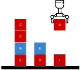
(a) Grounded state.

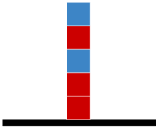
(b) Quantified goal.

Figure 1: A Blocks example. The goal shown on the right is: $\exists x_{1},\dots x_{5}:\textsc{Blue}(x_{1})\wedge\textsc{Red}(x_{2})\wedge\textsc{Blue}(x_{3})\wedge\textsc{Red}(x_{4})\wedge\textsc{Red}(x_{5})\wedge\textsc{On}(x_{1},x_{2})\wedge\textsc{On}(x_{2},x_{3})\wedge\textsc{On}(x_{3},x_{4})\wedge\textsc{On}(x_{4},x_{5})$. The cost of an optimal goal grounding is 9. In the experiments, our learned model instead finds a suboptimal goal grounding with a cost of 15.

Blocks is the standard Blockworld domain with a gripper and block colors that can be used in the goals. Figure 1 depicts an instance of the domain involving 8 blocks, named from $A$ to $H$, and expressed as:

$$\exists x_{1},\ldots,x_{5}:\; \textsc{Blue}(x_{1})\wedge\textsc{Red}(x_{2})\wedge\textsc{Blue}(x_{3})$$

$$\wedge\textsc{Red}(x_{4})\wedge\textsc{Red}(x_{5})\wedge\textsc{On}(x_{1},x_{2})$$

$$\wedge\textsc{On}(x_{2},x_{3})\wedge\textsc{On}(x_{3},x_{4})\wedge\textsc{On}(x_{4},x_{5}).$$

This goal requires constructing a tower in which a blue block $x_{1}$ rests on a red block $x_{2}$, which in turn rests on a blue block $x_{3}$, which rests on a red block $x_{4}$, and finally, that rests on another red block $x_{5}$. The optimal grounding involves binding block $x_{5}$ to block $F$ and block $x_{4}$ to block $A$, so that the target tower is built on top of $F$.

Let us emphasize that the grounding problem tackled by the learner is not easy. Firstly, the resulting binding needs to be logically valid, meaning it must adhere to the static constraints of the goal, such as colors in this case. A binding would be logically invalid if a variable $x_{i}$ is bound to a constant $c$ with a different color from $x_{i}$ in the goal. Secondly, the resulting binding must lead to a reachable goal. In this domain, it implies that no pair of variables $x_{i}$ can be bound to the same constant, as the blocks $x_{i}$ need to form a single tower. Lastly, the resulting binding needs to be optimal; that is, it must be achievable in the fewest steps possible. None of these three properties – validity, reachability, or optimality – are hardcoded or guaranteed by the learning architecture, but we can experimentally test them. Planners that handle existentially quantified goals by expanding them into grounded DNF formulas ensure and exploit validity. By pruning the DNF terms that are not logically valid, they exploit (but do not guarantee) reachability by removing DNF clauses containing mutually exclusive atom pairs. They ensure optimality if they are optimal planners. In our setting, validity, reachability, and optimality, or a reasonable approximation, must be learned solely from training.

The domain called Blocks-C is essentially the same as the Blocks domain, but instead of focusing on the relation On, it revolves around the relation Clear. This implies that the goal is to dismantle towers to uncover blocks of specific colors, with the fewest steps possible.

9.2 Gripper

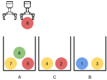
(a) Grounded state.

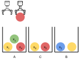
(b) Predicted grounding.

Figure 2: A Gripper example. The goal is: $\exists x_{1},\ldots,x_{4}:\big{[}\textsc{Yellow}(x_{1})\wedge\textsc{Blue}(x_{2})\wedge\textsc{Green}(x_{3})\wedge\textsc{Red}(x_{4})\wedge\textsc{Red}(x_{5})\wedge\textsc{Yellow}(x_{6})\wedge\textsc{At}(x_{1},A)\wedge\textsc{At}(x_{2},A)\wedge\textsc{At}(x_{3},B)\wedge\textsc{At}(x_{4},A)\wedge\textsc{At}(x_{5},C)\wedge\textsc{At}(x_{6},C)\big{]}\wedge\big{[}\bigwedge_{i,j}\textsc{Neq}(x_{i},x_{j})\big{]}$, where $\textsc{Neq}(x,y)$ denotes that $x$ and $y$ have to be different constants. The grounding of the goal that our learned model predicts is shown on the right. This is an optimal binding with a cost of 8.

In Gripper, there is a robot equipped with two grippers that can pick up balls and move them between rooms. In our version, the balls are colored, and there is a fixed number of rooms that are not necessarily adjacent to each other. Figure 2 provides an example. In this figure, there are three rooms labeled as $A$, $B$, and $C$. The goal is:

$$\exists x_{1},\ldots,x_{4}:\; \textsc{Yellow}(x_{1})\wedge\textsc{Blue}(x_{2})\wedge\textsc{Green}(x_{3})$$

$$\wedge\textsc{Red}(x_{4})\wedge\textsc{Red}(x_{5})\wedge\textsc{Yellow}(x_{6})$$

$$\wedge\textsc{At}(x_{1},A)\wedge\textsc{At}(x_{2},A)\wedge\textsc{At}(x_{3},B)$$

$$\wedge\textsc{At}(x_{4},A)\wedge\textsc{At}(x_{5},C)\wedge\textsc{At}(x_{6},C)$$

$$\wedge\big{[}\bigwedge_{i,j}\textsc{Neq}(x_{i},x_{j})\big{]}$$

The goal is to place a yellow ball $x_{1}$, a blue ball $x_{2}$ and a red ball $x_{4}$ in room A, a green ball $x_{3}$ in room B, and a red ball $x_{5}$ and a yellow ball $x_{6}$ in room C. The optimal solution is to bind $x_{1}$ to $7$, $x_{4}$ to $5$, $x_{5}$ to $2$ and $x_{6}$ to $4$, since then the goal atoms with these variables are already true in the initial state. As for $x_{2}$ and $x_{3}$, these need to be bound to $1$ and $8$ respectively, since these are the only balls of the correct color.

9.3 Delivery

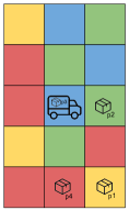
(a) Grounded state.

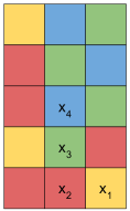
(b) Predicted grounding.

Figure 3: A Delivery example. The goal is: $\exists x_{1},\dots,x_{4}:\textsc{At}(p_{1},x_{3})\wedge\textsc{At}(p_{3},x_{2})\wedge\textsc{At}(p_{4},x_{1})\wedge\textsc{At}(t,x_{4})\wedge\textsc{Yellow}(x_{1})\wedge\textsc{Red}(x_{2})\wedge\textsc{Green}(x_{3})\wedge\textsc{Blue}(x_{4})\wedge\big{[}\bigwedge_{i,j}\textsc{Neq}(x_{i},x_{j})\big{]}$, where $\textsc{Neq}(x,y)$ denotes that $x$ and $y$ have to be different constants. Figure 3(b) shows the bindings of the learned model. This binding has a cost of 11, while LAMA produces a plan with a cost of 17.

In this domain, there is a truck, several packages, and a grid with colored cells. The goal is to distribute the packages to cells with specific colors. In the following example, there are $3$ packages, $p_{1}$, $p_{2}$, and $p_{3}$, to be distributed using truck $t$:

$$\exists x_{1},\dots,x_{4}:\; \textsc{At}(p_{1},x_{3})\wedge\textsc{At}(p_{3},x_{2})\wedge\textsc{At}(p_{4},x_{1})$$

$$\wedge\textsc{At}(t,x_{4})\wedge\textsc{Yellow}(x_{1})\wedge\textsc{Red}(x_{2})$$

$$\wedge\textsc{Green}(x_{3})\wedge\textsc{Blue}(x_{4})$$

$$\wedge\big{[}\bigwedge_{i,j}\textsc{Neq}(x_{i},x_{j})\big{]}$$

To distribute these packages efficiently, the truck must decide on an order to pick up the packages and deliver them to cells close to this planned route to minimize the total cost.

In this example, the truck must deliver package $p_{1}$ to a green cell $x_{3}$, $p_{3}$ to a red cell $x_{2}$, $p_{4}$ to a yellow cell $x_{1}$, and then park the truck $t$ in a blue cell $x_{4}$. As seen in Figure 3(b), the learned model selects cells close to where the packages are, which lowers the total distance traveled by the truck.

9.4 Visitall

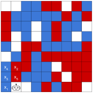
Figure 4: A Visitall example. The goal is: $\exists x_{1},\dots,x_{5}:\big{[}\textsc{Blue}(x_{1})\wedge\textsc{Blue}(x_{3})\wedge\textsc{Blue}(x_{4})\wedge\textsc{Red}(x_{2})\wedge\textsc{Red}(x_{5})\wedge\textsc{Visited}(x_{1})\wedge\textsc{Visited}(x_{2})\wedge\textsc{Visited}(x_{3})\wedge\textsc{Visited}(x_{4})\wedge\textsc{Visited}(x_{5})\big{]}\wedge\big{[}\bigwedge_{i,j}\textsc{Neq}(x_{i},x_{j})\big{]}$, where $\textsc{Neq}(x,y)$ denotes that $x$ and $y$ have to be different constants. An optimal grounding with a cost of $5$ is shown. In this case, LAMA fails to find a solution within the time limit, but when combined with our learned model, it solves the resulting grounded instance optimally.

In a more general version of Visit-1, presented in Section 2, the robot is required to visit at least one cell of each color specified in the goal while also minimizing the total distance traveled. Figure 4 provides an example. The example goal is:

$$\exists x_{1},\dots,x_{5}:\big{[} \textsc{Blue}(x_{1})\wedge\textsc{Blue}(x_{3})\wedge\textsc{Blue}(x_{4})$$

$$\wedge\textsc{Red}(x_{2})\wedge\textsc{Red}(x_{5})\wedge\textsc{Visited}(x_{1})$$

$$\wedge\textsc{Visited}(x_{2})\wedge\textsc{Visited}(x_{3})$$

$$\wedge\textsc{Visited}(x_{4})\wedge\textsc{Visited}(x_{5})\big{]}$$

$$\wedge\big{[}\bigwedge_{i,j}\textsc{Neq}(x_{i},x_{j})\big{]}$$

The robot needs to visit 3 blue cells $x_{1}$, $x_{3}$, and $x_{4}$, and 2 red cells $x_{2}$ and $x_{5}$. An optimal solution with a cost of $5$ is shown in Figure 4. This domain poses a difficult optimization problem, similar to but distinct from the Traveling Salesman Problem (TSP).

		No $x_{i}\neq x_{j}$ constraint			With $x_{i}\neq x_{j}$ constraints			Random groundings
Domain	#	Cov.	$V^{*}$	$V/V^{*}$	Cov.	$V^{*}$	$V/V^{*}$	All Cov.	Valid Cov.	$V/V^{*}$
Blocks	500	99.8 %	8.918	1.211	99.8 %	8.918	1.211	3.8 %	76.2 %	1.391
Blocks-C	500	99.8 %	3.402	1.103	100 %	4.478	1.019	6.8 %	100 %	1.797
Gripper	500	100 %	4.78	1.298	99.4 %	5.304	1.189	3 %	86.6 %	1.499
Delivery	500	99.8 %	9.016	1.238	100 %	9.224	1.177	10.8 %	100 %	1.522
Visitall	500	100 %	4.072	1.181	99.2 %	4.712	1.080	2.6 %	100 %	1.445

Table 1: This table shows how well the learned model performed on the optimal test sets (refer to Table 2). For each domain, we evaluate the learned models in two settings: one where multiple variables assigned to the same object can result in valid bindings, and one where these are always invalid. These settings are labeled as ”No $x_{i}\neq x_{j}$ constraint” and ”With $x_{i}\neq x_{j}$ constraints,” respectively. The ”#” column indicates the number of test instances. The performance of the learned models is displayed as coverage (Cov.), which represents the percentage of instances solved after grounding the goal. The average cost of optimal plans is shown in the $V^{*}$ column, and the quality of the grounded goal is presented as the ratio between the cost of the plan found using the grounded goal and the cost of an optimal plan in the $V/V^{*}$ column. Additionally, we compare the results to two baselines where groundings are randomly sampled: one considering all possible bindings and another considering only those that satisfy static constraints (e.g., colors). These baselines are labeled as ”Random groundings,” with ”All” and ”Valid” denoting the two methods, respectively. The quality ratio presented in $V/V^{*}$ corresponds to the ”Valid” baseline.

		Optimal	LAMA
Domain	Train	Test	Test
Blocks	[2, 7]	8	[9, 17]
Blocks-C	[2, 7]	8	[9, 17]
Gripper	[9, 11]	13	[15,47]
Delivery	[6, 25]	[26, 30]	[31, 88]
Visitall	[2, 16]	20	[25, 100]

Table 2: An overview of the different datasets used in our experiments. The intervals represent the number of constants appearing in the states. For instance, we train a model using up to $7$ blocks for the Blocks domain. Subsequently, we evaluate this model on two different test sets: one where we were able to compute the cost of an optimal binding, labeled as Optimal, and another where the cost is determined using the LAMA planner, labeled as LAMA. In all domains, the training set includes instances with $1$ to $4$ goal variables, and the test data includes instances with $1$ to $6$ goal variables. The number of colors for each instance ranges from $1$ to $6$ for both the training and test sets.

		No $x_{i}\neq x_{j}$ constraint					With $x_{i}\neq x_{j}$ constraints
Domain	#	Cov.	LAMA Cov.	$V^{L}$	$V/V^{L}$	Speedup	Cov.	LAMA Cov.	$V^{L}$	$V/V^{L}$	Speedup
Blocks	500	100 %	99.4 %	11.93	1.245	19.837	100 %	99.2 %	11.93	1.245	19.837
Blocks-C	500	100 %	100 %	2.74	1.179	1.359	99.8 %	100 %	4.438	1.047	1.190
Gripper	500	97.6 %	96.2 %	6.368	1.263	104.335	99.6 %	97 %	7.07	1.239	68.306
Delivery	500	99 %	98.6 %	7.958	1.459	50.495	100 %	98.6 %	8.768	1.212	36.533
Visitall	500	100 %	98 %	4.884	1.480	33.219	88.8 %	96.6 %	5.306	1.122	43.468

Table 3: This table shows the performance of the learned model on the LAMA test sets (refer to Table 2). See Table 1 for explanations of most columns. We were unable to compute $V^{*}$ for these instances, so we approximate it using LAMA, denoted as $V^{L}$. We evaluate two configurations: first, LAMA using grounded goals obtained through our learned models, and second, LAMA using the quantified goal. The coverage of the first and second configurations is presented in the ”Cov.” and ”LAMA Cov.” columns, respectively. The ”Speedup” column illustrates the speedup of using the first configuration over the second.

10 Experimental Results

Once a model has been trained to predict the cost of partially quantified goals relative to a state, it is then possible to use it as a policy. If $V$ is a learned model for some domain, then it defines a policy $\pi_{V}$ over the space of partially quantified goals as follows. Let $s$ and $G$ be a state and a goal, respectively; the successors $N(s,G)$ of $s$ and $G$ are a set of goals where $G$ has bound a single variable with a constant. The policy $\pi_{V}$ is:

$$\pi_{V}(s,G)=\operatorname*{arg\,min}_{G_{x=c}\in N(s,G)}V(s,G_{x=c}).$$

The policy is iteratively used until the goal is fully grounded. By binding a single variable, we avoid the combinatorial explosion that would occur when considering all possible combinations. The number of iterations required to fully ground $G$ is equal to the number of variables.

We implemented the proposed method using PyTorch and trained the models on NVIDIA A10 GPUs with 24 GB of memory. Training lasted a maximum of $100~{}000$ epochs or $72$ hours. We used Adam (?) with a learning rate of $0.001$, using batch sizes ranging from $1024$ to $8192$. Each domain’s dataset comprised $40~{}000$ pairs of states and goals, $39~{}500$ for training and 500 for validation. The number of constants used in both the training and testing sets are detailed in Table 2. During training, we used up to $4$ variables, while during testing, we used up to $6$. Furthermore, the trained models support up to $6$ distinct colors. The learned models have $30$ layers and an embedding size of $32$. For each specific domain, we trained a single model and the model with the lowest validation loss was used for testing.

10.1 Results

As mentioned earlier, our goal is to learn goal groundings that are: logically valid, reachable, and efficient (close to optimal). Tables 1 and 3 show the performance of our learned models across various domains. Tables 4 and 5 delve deeper into two specific domains, Blocks and Visitall, illustrating how well the learned models scale and generalize with an increasing number of constants. We discuss how the experiments shed light on these properties.

Validity and reachabilty. A valid grounding is one that satisfies static constraints, such as colors. For instance, the learned models are permitted to bind a variable to a red block even if that variable must be bound to a blue block. If this occurs, the resulting grounded goal is unsatisfiable, leading to an unsolvable instance. In Tables 1 and 3, the coverage measures this property, as all solvable groundings must also be valid. However, a valid grounding does not necessarily have to be reachable from the given state. The coverage measures that the goal groundings are both valid and reachable. In our experiments, our learned models result in a system with very high coverage, meaning that the vast majority of the goal groundings are both valid and reachable. Additionally, in Table 1, the baseline ”All Cov.” shows that randomly grounding variables will likely result in an invalid grounding. The other baseline, ”Valid Cov.”, randomly selects a valid grounding, ensuring validity but not reachability. However, it often leaves Blocks and Gripper instances unsolvable. In contrast, our learned models produce goal groundings that are both valid and reachable.

Efficiency. We evaluate efficiency in two datasets. Firstly, in Table 1, we compare the actual cost of predicted goal groundings, denoted as $V$, to the optimal cost of goal groundings, denoted as $V^{*}$. Secondly, in Table 3, where determining $V^{*}$ is computationally infeasible, we instead compare against the plan length identified by LAMA (?). These comparisons are presented as the quotients $V/V^{*}$ and $V/V^{L}$ in Tables 1 and 3, respectively. We observe that our goal groundings are often close to optimal for smaller instances, with averages reaching up to $1.238$. For larger instances requiring LAMA, goal groundings degrade a bit, with averages reaching up to $1.48$. It is important to note that these ratios are calculated only over instances solvable by both LAMA alone and LAMA with our learned models and that LAMA does not necessarily find an optimal plan for grounded goals. Tables 4 and 5 show whether the quality of the goal groundings deteriorates as the instance size increases in two domains: Blocks and Visitall. It seems that the quality does not degrade, as it remains consistent when the number of constants increases.

Scalability. LAMA compiles quantified goals by expanding them into grounded DNF formulas, whose clauses become the conditions of axioms that derive a new dummy atom. This expansion is exponential in the number of goal variables, takes preprocessing time, and affects the quality of the resulting heuristic. As a result, if LAMA is given a high-quality grounded goal, it can avoid preprocessing and get a more informed heuristic. The column labeled ”Speedup” in Tables 1 and 3 indicates the speedup achieved by running LAMA with our learned models compared to LAMA alone. We observe a two-order-of-magnitude speedup in the Gripper domain in Table 3, and in most domains, we see a one-order-of-magnitude speedup. Furthermore, in Tables 4 and 5, instances are aggregated based on size (# constants) rather than by domain. This allows us to observe scalability in the Blocks and Visitall domains, demonstrating that the speedup increases with the instance size. In Table 5, as the number of objects becomes very large, the coverage decreases for both LAMA alone and LAMA with the learned model: in the first case, the search times out; in the second, unreachable grounded goals are generated.

Size	#	Cov.	L. Cov.	$V^{L}$	$V/V^{L}$	Speedup
7	33	100 %	100 %	18.485	1.131	0.453
9	33	100 %	100 %	15.939	1.399	4.207
11	31	100 %	100 %	14.645	1.198	16.818
13	27	100 %	100 %	14.111	1.491	1.843
15	33	100 %	100 %	11.545	1.247	6.964
17	29	100 %	93.1 %	11.778	1.476	136.028

Table 4: Performance and generalization scaling within the domain of Blocks. The instances are scaled by the number of constants (blocks), as shown in the column labeled ”Size”. Refer to Table 3 for explanations of the other columns. Note that, the largest instance in the training set consists of exactly 7 constants. Therefore, this table also illustrates how well the learned models generalize beyond the training distribution.

Size	#	Cov.	L. Cov.	$V^{L}$	$V/V^{L}$	Speedup
16	27	96.3	100	5.444	1.003	0.788
20	25	100	100	6.36	1.126	1.775
25	25	96	100	6.0	1.132	5.333
49	21	71.4	95.2	8.2	0.911	13.813
64	32	56.3	81.3	7.577	1.027	14.996
100	36	61.1	80.6	4.690	1.386	8.513

Table 5: Performance and generalization scaling within the domain of Visitall. See Table 4 for explanations of the columns.

11 Analysis: Visit-Many

We now continue the example from Section 2 and present a detailed analysis where a specific number of colors must be visited. In our experiments, we allow the number of colors in the goal to vary, but here we assume exactly $k$ colors:

$$\exists x_{1},\dots,x_{k}:\textsc{C}_{1}(x_{1})\wedge\dots\wedge\textsc{C}_{k}(x_{k}),\text{where }\textsc{C}_{i}\in\mathcal{C}.$$

To determine distances, we adjust the Boolean functions P and SP to check if there is a path of length $d$ that visits cells with colors $\langle\textsc{C}_{1},\dots,\textsc{C}_{n}\rangle$ in the specified order:

$$\text{P}_{0,C}(x) =\textsc{C}(x),$$

$$\text{P}_{d,\langle\textsc{C}_{1},\dots,\textsc{C}_{n}\rangle}(x) =\textsc{C}_{1}(x)\wedge P_{d,\textsc{C}_{2},\dots,\textsc{C}_{n}}(x),$$

$$\text{P}_{d,\langle\textsc{C}_{1},\dots,\textsc{C}_{n}\rangle}(x) =\exists y:\textsc{Conn.}(x,y)\wedge P_{d-1,\langle\textsc{C}_{1},\dots,\textsc{C}_{n}\rangle}(y),$$

$$\text{SP}_{d,\langle\textsc{C}_{1},\dots,\textsc{C}_{n}\rangle}(x) =\text{P}_{d,\langle\textsc{C}_{1},\dots,\textsc{C}_{n}\rangle}(x)\wedge\neg\text{P}_{d-1,\langle\textsc{C}_{1},\dots,\textsc{C}_{n}\rangle}(x).$$

The colors in the subscript act like a queue: if the color of the current cell matches the color in front of the queue, that color is removed. The value function is then defined as:

$$\textsc{G}_{\bar{\textsc{C}}} =\neg\exists\textsc{C}\in\mathcal{C}\setminus\bar{\textsc{C}}:\left[\exists v:\textsc{C}_{G}(v)\right],$$

$$\text{D}_{d,\bar{\textsc{C}}} =\textsc{G}_{\bar{\textsc{C}}}\wedge\exists x:\left[\textsc{At-Robot}(x)\wedge\text{SP}_{d,\bar{\textsc{C}}}(x)\right],$$

$$V^{*}(s;G) =\min_{d\in\mathcal{D},\bar{\textsc{C}}\in\mathcal{C}^{k}}d\cdot[\![\text{D}_{d,\bar{\textsc{C}}}]\!]+N\cdot[\![\neg D_{d,\bar{\textsc{C}}}]\!].$$

Here, $\mathcal{D}$ is the fixed set of distances, $\mathcal{C}$ is the fixed set of all colors, and $\mathcal{C}^{k}$ is the set of all ordered sequences of length $k$, where each element is chosen from $\mathcal{C}$ (elements can be repeated). The $\textsc{G}_{\bar{\textsc{C}}}$ feature is false when the goal involves a color not in the sequence $\bar{\textsc{C}}$. This is because both the goal and the sequence allow for repetition. Since the number of colors is fixed, we can expand the outer quantifier. We assume that the given state does not contain any Visited atoms, since grounding should be done on the initial state. If there is such an atom, $V^{*}$ may return a suboptimal value.

No more than two variables are used at any point, indicating that this domain with such quantified goals belongs to $C_{2}$. Note that this analysis excludes any inequality constraints, which might move the task outside of $C_{2}$.

12 Conclusions

We considered the problem of learning to ground existentially quantified goals, building on existing techniques for learning general policies using GNNs. These methods usually require goals that are already grounded, and the aim is to enable them to support existentially quantified goals by grounding them beforehand. This preprocessing step is also useful for classical planning, where existentially quantified goals exponentially increase time and space requirements. We also discuss this approach in relation to $C_{2}$ logics, as it builds on relational GNNs for representing and learning general value functions (?).

Grounding existentially quantified goals after learning is computationally efficient and does not require search. The process involves greedily following the learned value function, substituting one variable at a time with a constant. However, learning such a value function is challenging because the grounded goals must satisfy conditions of logical validity, reachability, and optimality. We tested these conditions experimentally on instances with more objects, goal atoms, and variables. In the future, we plan to explore unsupervised methods for grounding learning, fine-tuning weights using reinforcement learning as done by (?), and experimenting with GNN architectures with improved expressive power (?; ?). This might include adding memory and recursion capabilities (?).

References

- Bajpai, Garg, and others 2018 Bajpai, A. N.; Garg, S.; et al. 2018. Transfer of deep reactive policies for mdp planning. In Proc. of the 32nd Annual Conference on Neural Information Processing Systems (NeurIPS 2018), 10965–10975.
- Barceló et al. 2020 Barceló, P.; Kostylev, E.; Monet, M.; Pérez, J.; Reutter, J.; and Silva, J.-P. 2020. The logical expressiveness of graph neural networks. In Proc. of the 8th International Conference on Learning Representations (ICLR 2020).
- Cai, Fürer, and Immerman 1992 Cai, J.-Y.; Fürer, M.; and Immerman, N. 1992. An optimal lower bound on the number of variables for graph identification. Combinatorica 12(4):389–410.
- Chevalier-Boisvert et al. 2019 Chevalier-Boisvert, M.; Bahdanau, D.; Lahlou, S.; Willems, L.; Saharia, C.; Nguyen, T. H.; and Bengio, Y. 2019. Babyai: A platform to study the sample efficiency of grounded language learning. In Proc. of the 7th International Conference on Learning Representations (ICLR 2019). OpenReview.net.
- Corrêa et al. 2020 Corrêa, A. B.; Pommerening, F.; Helmert, M.; and Francès, G. 2020. Lifted successor generation using query optimization techniques. In Proc. of the 30th International Conference on Automated Planning and Scheduling (ICAPS 2020), 80–89. AAAI Press.
- Fern, Yoon, and Givan 2006 Fern, A.; Yoon, S.; and Givan, R. 2006. Approximate policy iteration with a policy language bias: Solving relational markov decision processes. Journal of Artificial Intelligence Research 25:75–118.
- Frances and Geffner 2015 Frances, G., and Geffner, H. 2015. Modeling and computation in planning: Better heuristics from more expressive languages. In Proc. of the 25th International Conference on Automated Planning and Scheduling (ICAPS 2015), 70–78. AAAI Press.
- Francès and Geffner 2016 Francès, G., and Geffner, H. 2016. -strips: Existential quantification in planning and constraint satisfaction. In Kambhampati, S., ed., Proc. of the 25th International Joint Conference on Artificial Intelligence (IJCAI 2016), 3082–3088. AAAI Press.
- Francès et al. 2019 Francès, G.; Corrêa, A. B.; Geissmann, C.; and Pommerening, F. 2019. Generalized potential heuristics for classical planning. In Proc. of the 28th International Joint Conference on Artificial Intelligence (IJCAI 2019), 5554–5561. IJCAI.
- Francès, Bonet, and Geffner 2021 Francès, G.; Bonet, B.; and Geffner, H. 2021. Learning general planning policies from small examples without supervision. In Proc. of the 35th AAAI Conference on Artificial Intelligence (AAAI 2021), 11801–11808. AAAI Press.
- Gazen and Knoblock 1997 Gazen, B. C., and Knoblock, C. A. 1997. Combining the expressivity of UCPOP with the efficiency of Graphplan. In Recent Advances in AI Planning. 4th European Conference on Planning (ECP 1997), volume 1348 of Lecture Notes in Artificial Intelligence, 221–233. Springer-Verlag.
- Geffner and Bonet 2013 Geffner, H., and Bonet, B. 2013. A Concise Introduction to Models and Methods for Automated Planning, volume 7 of Synthesis Lectures on Artificial Intelligence and Machine Learning. Morgan & Claypool.
- Ghallab, Nau, and Traverso 2016 Ghallab, M.; Nau, D.; and Traverso, P. 2016. Automated planning and acting. Cambridge U.P.
- Gilmer et al. 2017 Gilmer, J.; Schoenholz, S. S.; Riley, P. F.; Vinyals, O.; and Dahl, G. E. 2017. Neural message passing for quantum chemistry. In Proc. of the 34th International Conference on Machine Learning (ICML 2017), 1263–1272. JMLR.org.
- Grohe 2021 Grohe, M. 2021. The logic of graph neural networks. In Proceedings of the Thirty-Sixth Annual ACM/IEEE Symposium on Logic in Computer Science (LICS 2021), 1–17.
- Hamilton 2020 Hamilton, W. 2020. Graph Representation Learning, volume 14 of Synthesis Lectures on Artificial Intelligence and Machine Learning. Morgan & Claypool.
- Haslum et al. 2019 Haslum, P.; Lipovetzky, N.; Magazzeni, D.; and Muise, C. 2019. An Introduction to the Planning Domain Definition Language, volume 13 of Synthesis Lectures on Artificial Intelligence and Machine Learning. Morgan & Claypool.
- Illanes and McIlraith 2019 Illanes, L., and McIlraith, S. A. 2019. Generalized planning via abstraction: Arbitrary numbers of objects. In Proc. of the 33rd AAAI Conference on Artificial Intelligence (AAAI 2019), 7610–7618. AAAI Press.
- Khardon 1999 Khardon, R. 1999. Learning action strategies for planning domains. Artificial Intelligence 113:125–148.
- Kingma and Ba 2015 Kingma, D. P., and Ba, J. 2015. Adam: A method for stochastic optimization. In Proc. of the 3rd International Conference on Learning Representations (ICLR 2015).
- Martín and Geffner 2004 Martín, M., and Geffner, H. 2004. Learning generalized policies from planning examples using concept languages. Applied Intelligence 20(1):9–19.
- Misra 2020 Misra, D. 2020. Mish: A self regularized non-monotonic activation function. In Proceedings of the 31st British Machine Vision Conference (BMVC 2020). BMVA Press.
- Morris et al. 2019 Morris, C.; Ritzert, M.; Fey, M.; Hamilton, W. L.; Lenssen, J. E.; Rattan, G.; and Grohe, M. 2019. Weisfeiler and leman go neural: Higher-order graph neural networks. In Proc. of the 33rd AAAI Conference on Artificial Intelligence (AAAI 2019), 4602–4609. AAAI Press.
- Narasimhan, Barzilay, and Jaakkola 2018 Narasimhan, K.; Barzilay, R.; and Jaakkola, T. 2018. Grounding language for transfer in deep reinforcement learning. Journal of Artificial Intelligence Research 63:849–874.
- Pednault 1989 Pednault, E. P. D. 1989. ADL: Exploring the middle ground between STRIPS and the situation calculus. In Proc. of the 1st International Conference on Principles of Knowledge Representation and Reasoning (KR 1989), 324–332. Morgan Kaufmann.
- Pfluger, Cucala, and Kostylev 2024 Pfluger, M.; Cucala, D. T.; and Kostylev, E. V. 2024. Recurrent graph neural networks and their connections to bisimulation and logic. In Proc. of the 38th AAAI Conference on Artificial Intelligence (AAAI 2024), volume 38, 14608–14616. AAAI Press.
- Richter and Westphal 2010 Richter, S., and Westphal, M. 2010. The LAMA planner: Guiding cost-based anytime planning with landmarks. Journal of Artificial Intelligence Research 39:127–177.
- Rivlin, Hazan, and Karpas 2020 Rivlin, O.; Hazan, T.; and Karpas, E. 2020. Generalized planning with deep reinforcement learning. In ICAPS 2020 Workshop on Bridging the Gap Between AI Planning and Reinforcement Learning (PRL), 16–24.
- Ruis et al. 2020 Ruis, L.; Andreas, J.; Baroni, M.; Bouchacourt, D.; and Lake, B. M. 2020. A benchmark for systematic generalization in grounded language understanding. In Larochelle, H.; Ranzato, M.; Hadsell, R.; Balcan, M.; and Lin, H., eds., Proc. of the 34th Annual Conference on Neural Information Processing Systems (NeurIPS 2020), volume 33, 19861–19872. Curran Associates, Inc.
- Scarselli et al. 2009 Scarselli, F.; Gori, M.; Tsoi, A. C.; Hagenbuchner, M.; and Monfardini, G. 2009. The graph neural network model. IEEE Transactions on Neural Networks 20(1):61–80.
- Srivastava, Immerman, and Zilberstein 2011 Srivastava, S.; Immerman, N.; and Zilberstein, S. 2011. A new representation and associated algorithms for generalized planning. Artificial Intelligence 175(2):393–401.
- Ståhlberg, Bonet, and Geffner 2022a Ståhlberg, S.; Bonet, B.; and Geffner, H. 2022a. Learning general optimal policies with graph neural networks: Expressive power, transparency, and limits. In Proc. of the 32nd International Conference on Automated Planning and Scheduling (ICAPS 2022), 629–637. AAAI Press.
- Ståhlberg, Bonet, and Geffner 2022b Ståhlberg, S.; Bonet, B.; and Geffner, H. 2022b. Learning generalized policies without supervision using GNNs. In Proc. of the 19th International Conference on Principles of Knowledge Representation and Reasoning (KR 2022), 474–483. IJCAI Organization.
- Ståhlberg, Bonet, and Geffner 2023 Ståhlberg, S.; Bonet, B.; and Geffner, H. 2023. Learning general policies with policy gradient methods. In Proc. of the 20th International Conference on Principles of Knowledge Representation and Reasoning (KR 2023). IJCAI Organization.
- Ståhlberg 2023 Ståhlberg, S. 2023. Lifted successor generation by maximum clique enumeration. In Proc. of the 26th European Conference on Artificial Intelligence (ECAI 2023), 2194–2201. IOS Press.
- Toenshoff et al. 2021 Toenshoff, J.; Ritzert, M.; Wolf, H.; and Grohe, M. 2021. Graph neural networks for maximum constraint satisfaction. Frontiers in Artificial Intelligence and Applications 3:580607.
- Toyer et al. 2020 Toyer, S.; Thiébaux, S.; Trevizan, F.; and Xie, L. 2020. ASNets: Deep learning for generalised planning. Journal of Artificial Intelligence Research 68:1–68.
- Xu et al. 2019 Xu, K.; Hu, W.; Leskovec, J.; and Jegelka, S. 2019. How powerful are graph neural networks? In Proc. of the 7th International Conference on Learning Representations (ICLR 2019). OpenReview.net.