Bootstrap-based goodness-of-fit test for parametric families of conditional distributions

Abstract

In various scientific fields, researchers are interested in exploring the relationship between some response variable $Y$ and a vector of covariates $X$. In order to make use of a specific model for the dependence structure, it first has to be checked whether the conditional density function of $Y$ given $X$ fits into a given parametric family. We propose a consistent bootstrap-based goodness-of-fit test for this purpose. The test statistic traces the difference between a nonparametric and a semi-parametric estimate of the marginal distribution function of $Y$. As its asymptotic null distribution is not distribution-free, a parametric bootstrap method is used to determine the critical value. A simulation study shows that, in some cases, the new method is more sensitive to deviations from the parametric model than other tests found in the literature. We also apply our method to real-world datasets.

Keywords: model check, specification test, regression, Monte Carlo simulation

1 Introduction

In many scientific applications a response variable together with a number of features that possibly influence the outcome are observed. It is of high interest to figure out in which way the response (random) variable $Y$ depends on the vector of input (random) variables $X$. In this paper, we will propose a test to check whether the conditional distribution of $Y$ given $X$ fits into a given parametric family. According to Andrews (1997), many models in micro-econometric and biometric applications are of this type, and Maddala (1983) and McCullagh & Nelder (1983) list numerous examples. A common class of parametric regression models used in practice are generalized linear models (GLMs). They were first introduced in Nelder & Wedderburn (1972) and later on thoroughly discussed in Fahrmeir et al. (2013); Fox & Weisberg (2018); Dikta & Scheer (2021). Note that, as opposed to classical regression which merely assumes a model for the conditional mean, we consider a model for the whole distribution of $Y$ given $X$. This enables us to not only predict the value of $Y$ for some new feature vector $X$ but, for example, also provide a confidence band for the estimate.

The literature on goodness-of-fit tests for conditional distributions and related model checks for parametric families of regression functions is very extensive. The methods can be categorized into two general approaches, namely those that do make use of nonparametric kernel estimators and those that do not. Representatives of the former class are, for example, given in Rodríguez-Campos et al. (1998); Zheng (2000); Fan et al. (2006); Pardo-Fernández et al. (2007); Cao & González-Manteiga (2008); Ducharme & Ferrigno (2012). Since methods of this type suffer from the problem of choosing an appropriate smoothing parameter, we suggest a model check that falls into the second category here.

As stated above, there has already been done a tremendous amount of research in this direction, e.g. in Andrews (1997); Stute (1997); Stute & Zhu (2002); Delgado & Stute (2008); Bierens & Wang (2012); Veazie & Ye (2020); Dikta & Scheer (2021). Most of the proposed methods involve the approximation of the critical value by a bootstrap method and many of them were shown to be consistent. Some of them were even extended to time series data or function-valued parameters (see Bai (2003); Rothe & Wied (2013); Troster & Wied (2021)).

In sec:def, we derive a new test statistic for the problem at hand. A result on the limit distribution of the underlying process is established in sec:asymp which, in theory, can be used to approximate the $p$-value for large sample sizes $n$. However, it turns out that the limit distribution is dependent on the true distributions of $X$ and $Y$ which are unknown. To circumvent this problem and still be able to approximate the $p$-value, we suggest a parametric bootstrap method and establish its asymptotic justification in sec:boot. The consistency of the resulting goodness-of-fit test is verified in sec:cons. In sec:appl, the finite sample behavior of our method is studied, applying the method to both simulated and real datasets and comparing the results to methods from the literature. The appendix provides the proofs of the results stated in the text.

2 Definition of the test statistic

Let $\{(X_{i},Y_{i})\}_{i=1}^{n}$ be an i.i.d. sample of covariates and response variables with distribution function $H$ for $X$ and conditional density function $f(\,\cdot\,|x)$ for $Y$ given $X=x$ with respect to a $\sigma$-finite measure $\nu$. We want to create a test for

$$H_{0}:f\in\mathcal{F}=\{(x,y)\mapsto f(y|\vartheta,x)~{}|~{}\vartheta\in\Theta\}\quad\text{vs.}\quad H_{1}:f\notin\mathcal{F},$$ (1)

where

$$\Theta\coloneqq\left\{\vartheta\,\Big{|}\,\int\int f(y|\vartheta,x)\nu(dy)H(dx)<\infty\right\}$$

defines the set of admissible parameters. If $H_{0}$ holds, we denote the true distribution parameter by $\vartheta_{0}$.

Our test statistic will be based on the difference between a non-parametric and a semi-parametric estimate of the marginal distribution function $F_{Y}$ of $Y$. A natural choice for the non-parametric estimator is the empirical distribution function (ecdf) $\hat{F}_{Y,n}$ of $Y_{1},\dots,Y_{n}$. For the derivation of the estimator of $F_{Y}$ taking the assumed parametric family $\mathcal{F}$ for the conditional density function $f$ into account, we first rewrite

$$F_{Y}(t) =\mathbb{E}\left[{{I_{\left\{Y\leq t\right\}}}}\right]=\mathbb{E}\left[\mathbb{E}\left[{{I_{\left\{Y\leq t\right\}}}}\,|\,X\right]\right]$$

$$=\int\mathbb{E}\left[{{I_{\left\{Y\leq t\right\}}}}\,|\,X=x\right]H(dx)$$

$$=\int F(t|x)H(dx),$$

where $F(\,\cdot\,|x)$ is the true conditional distribution function of $Y$ given $X=x$. The semi-parametric estimate of $F_{Y}$ now follows in two approximation steps. First, we substitute the true conditional distribution with a parametric estimate, yielding

$$F_{Y,\hat{\vartheta}_{n}}(t)\coloneqq\int F\big{(}t|\hat{\vartheta}_{n},X_{i}\big{)}H(dx).$$

A classical choice for $\hat{\vartheta}_{n}$ is the maximum likelihood estimator (MLE). Our analysis is, however, worded in general terms and only requires the estimator to meet certain assumptions. As in most applications the distribution of the covariates is unknown, we further approximate $H$ by the ecdf $\hat{H}_{n}$ of $X_{1},\dots,X_{n}$, resulting in

$$\hat{F}_{Y,\hat{\vartheta}_{n}}(t)\coloneqq\int F(t|\hat{\vartheta}_{n},x)\hat{H}_{n}(dx)=\frac{1}{n}\sum_{i=1}^{n}F\big{(}t|\hat{\vartheta}_{n},X_{i}\big{)}.$$

Now, we define the conditional empirical process with estimated parameters as

$$\tilde{\alpha}_{n}(t) \coloneqq\sqrt{n}\left(\hat{F}_{Y,n}(t)-\hat{F}_{Y,\hat{\vartheta}_{n}}(t)\right)=\frac{1}{\sqrt{n}}\sum_{i=1}^{n}{{I_{\left\{Y_{i}\leq t\right\}}}}-F\big{(}t|\hat{\vartheta}_{n},X_{i}\big{)},\quad t\in\bar{\mathbb{R}}.$$

As a test statistic, we can use some continuous functional of the process $\tilde{\alpha}_{n}$. The supremum norm $\norm{\tilde{\alpha}_{n}}=\sup_{t\in\bar{\mathbb{R}}}\absolutevalue{\tilde{\alpha}_{n}(t)}$, for example, yields a Kolmogorov-Smirnov type statistic, whereas the integral $\int\tilde{\alpha}_{n}^{2}(t)F\big{(}t|\hat{\vartheta}_{n},dx\big{)}$ represents a Cramér-von-Mises type statistic. In the following, we will consider $\norm{\tilde{\alpha}_{n}}$ in particular but the results can be easily transferred to other statistics. The $p$-value corresponding to an observed test statistic value $A$ is given by

$$p\coloneqq\mathbb{P}_{H_{0}}(\norm{\tilde{\alpha}_{n}}\geq A).$$

As usual, the null hypothesis is rejected if the $p$-value is below some level of significance. In order to be able to compute the $p$-value (or equivalently the critical value), we need to know the distribution of $\norm{\tilde{\alpha}_{n}}$ under the null hypothesis.

3 Asymptotic null distribution

To investigate the asymptotic null distribution of our test statistic, we need to impose some conditions on the parametric model $\mathcal{F}$ and the estimator $\hat{\vartheta}_{n}$.

Assumption M1.

Define $v(t,\vartheta,x)\coloneqq\frac{\partial}{\partial\vartheta}f(t|\vartheta,x)=\left(v_{1}(t,\vartheta,x),\dots,v_{q}(t,\vartheta,x)\right)^{T}$.

1. There exists a neighborhood $V\subseteq\Theta$ of $\vartheta_{0}$ in which $v(t,\vartheta,x)$ is defined and there is a function $g(t,x)$ such that $\absolutevalue{v_{k}(t,\vartheta,x)}\leq g(t,x)$ for all $k=1,\dots,q$ and $\vartheta\in V$ with $\int g(t,x)\nu(dt)<\infty$ for $H$-a.e. $x$.

2. For every $k=1,\dots,q$ and $V$ defined in (i), it holds

   $$\int\sup_{\vartheta\in V}\int\absolutevalue{v_{k}(t,\vartheta,x)}\nu(dt)H(dx)<\infty.$$

The first condition M1cond:v_ex_dom is analogous to Dikta & Scheer (2021, 6.4.3(iv) and (v)). In their book, the parametric regression function $m$ plays the role of the conditional density $f$ in our analysis. In Andrews (1997, assumption M1(i)), the conditional distribution function $F$ is assumed to be differentiable which is a slightly weaker assumption than $f$ being differentiable. A sufficient condition for ass:m1cond:v_ddom is $\int\int g(t,x)\nu(dt)H(dx)<\infty$ with $g$ defined in ass:m1cond:v_ex_dom.

Assumption M2.

Define $w(t,\vartheta,x)\coloneqq\frac{\partial}{\partial\vartheta}F(t|\vartheta,x)=\left(w_{1}(t,\vartheta,x),\dots,w_{q}(t,\vartheta,x)\right)^{T}$.

1. The family of functions $\{\vartheta\mapsto w(t,\vartheta,x)\}_{t\in\mathbb{R}}$ is equicontinuous at $\vartheta_{0}$ for $H$-a.e. $x$, meaning that for $H$-a.e. $x$ and every $\varepsilon>0$, there exists a $\delta\equiv\delta(x,\varepsilon)>0$ such that

   $$\sup_{t\in\mathbb{R}}\norm{w(t,\vartheta,x)-w(t,\vartheta_{0},x)}<\varepsilon\quad\text{if}\quad\norm{\vartheta-\vartheta_{0}}<\delta.$$

2. $W(t,\vartheta)\coloneqq\mathbb{E}\left[w(t,\vartheta,X)\right]$ is uniformly continuous in $t$ at $\vartheta_{0}$.

In Andrews (1997, M1(ii)), the uniform convergence of the arithmetic mean of $w$ to its expected value $W$ is explicitly required. We use ass:m1cond:v_ddom and M2cond:w_cont to prove this convergence. ass:m2cond:W_cont is the analogue of Andrews (1997, M1(iii)) and Dikta & Scheer (2021, 6.5.2(xi)).

Assumption E1.

1. There exists a function $L$ with $\mathbb{E}\left[L(X,Y;\vartheta_{0})\right]=0$ and existing covariance matrix such that

   $$\sqrt{n}(\hat{\vartheta}_{n}-\vartheta_{0})=n^{-1/2}\sum_{i=1}^{n}L(X_{i},Y_{i};\vartheta_{0})+o_{\mathbb{P}}(1).$$

2. $\hat{\vartheta}_{n}\to\vartheta_{0}$ wp1 as $n\to\infty$.

The estimator $\hat{\vartheta}_{n}$ admitting an asymptotic linear representation as assumed in E1cond:mle_lin is a classic condition for convergence theorems of parametric test statistics. Usually, it is fulfilled for least squares estimators or maximum likelihood estimates. For the MLE, a corresponding result was established in Dikta & Scheer (2021, Corollary 5.56). Technically, their setting was a little different in that they were considering parametric GLMs in particular but the results can be easily extended to general conditional distribution families.

The following theorem establishes a convergence result for the conditional empirical process with estimated parameters $\tilde{\alpha}_{n}$. Specifically, we consider weak convergence in the space of uniformly bounded functions on the extended real line $\ell^{\infty}(\bar{\mathbb{R}})$ as defined in Kosorok (2008, Ch. 7). The asymptotic distribution of the test statistic $\norm{\tilde{\alpha}_{n}}$ can be derived subsequently using the Continuous Mapping Theorem.

Theorem 1.

Under $H_{0}$ and Assumptions M1, M2 and E1cond:mle_lin, it holds that

$$\tilde{\alpha}_{n}\Rightarrow\tilde{\alpha}_{\infty}\quad\text{in }\ell^{\infty}(\bar{\mathbb{R}}),$$

where $\tilde{\alpha}_{\infty}$ is a centered Gaussian process with covariance function

$$K(s,t)= ~{}\mathbb{P}_{\vartheta_{0}}\left(Y\leq\min(s,t)\right)-\mathbb{E}\left[F(s|\vartheta_{0},X)F(t|\vartheta_{0},X)\right]$$

$$+W^{T}(t,\vartheta_{0})\mathbb{E}_{\vartheta_{0}}\left[\quantity(F(s|\vartheta_{0},X)-{{I_{\left\{Y\leq s\right\}}}})L(X,Y;\vartheta_{0})\right]$$

$$+W^{T}(s,\vartheta_{0})\mathbb{E}_{\vartheta_{0}}\left[\quantity(F(t|\vartheta_{0},X)-{{I_{\left\{Y\leq t\right\}}}})L(X,Y;\vartheta_{0})\right]$$

$$+W^{T}(s,\vartheta_{0})\text{COV}_{\vartheta_{0}}\left(L(X,Y;\vartheta_{0})\right)W(t,\vartheta_{0}).$$

As the asymptotic null distribution involves $\vartheta_{0}$ as well as the distribution of $X$, it is case dependent and cannot be tabulated. For that reason, we suggest a bootstrap method to approximate the limit distribution.

4 Parametric bootstrap method

The goal of bootstrap methods, in general, is to estimate the distribution of a given test statistic under the null hypothesis by generating new samples introducing some type of randomness while sticking as close as possible to the original sample. In our case, this means that we want to estimate the distribution of $\norm{\tilde{\alpha}_{n}}$ by generating new samples $\{(X_{i,n}^{*},Y_{i,n}^{*})\}$ whose conditional distribution is guaranteed to belong to the conditional distribution family $\mathcal{F}$ while at the same time keeping the distributions as similar as possible to the original sample. These considerations lead to the following resampling scheme:

1. Keep the covariates the same: $X_{i,n}^{*}=X_{i}$.

2. Generate new response variables $Y_{i,n}^{*}$ according to the estimated conditional distribution function $F\big{(}\cdot|\hat{\vartheta}_{n},X_{i,n}^{*}\big{)}$.

3. Based on this new bootstrap sample, find an estimate $\hat{\vartheta}_{n}^{*}$ for the distribution parameter.

4. Determine the bootstrap conditional empirical process with estimated parameters

   $$\tilde{\alpha}_{n}^{*}(t)\coloneqq\sqrt{n}\left(F^{*}_{Y,n}(t)-\hat{F}_{Y,\hat{\vartheta}_{n}^{*}}(t)\right),$$

   where $F^{*}_{Y,n}(t)$ denotes the ecdf of $\{Y_{i,n}^{*}\}_{i=1}^{n}$.

The $p$-value $\mathbb{P}_{H_{0}}\quantity(\norm{\tilde{\alpha}_{n}}\geq A)$ is then approximated by $\mathbb{P}_{n}^{*}\quantity(\norm{\tilde{\alpha}_{n}^{*}}\geq A)$ with $\mathbb{P}_{n}^{*}$ indicating the probability measure corresponding to the bootstrap random variables based on $n$ original observations. This approach is justified if the bootstrap process $\tilde{\alpha}_{n}^{*}$ converges to the same limit distribution as $\tilde{\alpha}_{n}$. To prove a corresponding result, some additional assumptions are needed.

Assumption M3.

For the neighborhood $V$ of $\vartheta_{0}$ defined in ass:m1, it holds that

$$\int\int\sup_{\vartheta\in V}f(y|\vartheta,x)\nu(dy)H(dx)<\infty.$$

This assumption is needed to apply Dikta & Scheer (2021, Lemma 5.58), a bootstrap weak law, whenever the integrand is absolutely bounded by one. It is used in several occasions in the proof but, compared to Dikta and Scheer’s book, it mainly replaces their condition 6.5.1(ii).

Assumption E2.

Let $L$ be the function defined in ass:e1.

1. $\sqrt{n}(\hat{\vartheta}_{n}^{*}-\hat{\vartheta}_{n})=n^{-1/2}\sum_{i=1}^{n}L(X_{i},Y_{i,n}^{*};\hat{\vartheta}_{n})+o_{\mathbb{P}_{n}^{*}}(1).$

2. $\mathbb{E}_{n}^{*}\left[L(X,Y^{*};\hat{\vartheta}_{n})\right]=0$ and

   $$\frac{1}{n}\sum_{i=1}^{n}\mathbb{E}_{n}^{*}\left[L(X_{i},Y_{i,n}^{*};\hat{\vartheta}_{n})L^{T}(X,Y_{i,n}^{*};\hat{\vartheta}_{n})\right]\xrightarrow[n\to\infty]{}\mathbb{E}_{\vartheta_{0}}\left[L(X,Y;\vartheta_{0})L^{T}(X,Y;\vartheta_{0})\right].$$

ass:e2 is usually fulfilled for appropriate estimators $\hat{\vartheta}_{n}$. Its validity for the MLE can be proven similarly as Dikta & Scheer (2021, Theorem 5.59 and Corollary 5.62).

Assumption E3.

Let $L$ be the function defined in ass:e1.

1. $L$ is continuous in $\vartheta$ at $\vartheta_{0}$ and there exist neighborhoods $V_{1}$ and $V_{2}$ of $\vartheta_{0}$ such that

   $$\int\int\sup_{\vartheta_{1}\in V_{1}}\norm{L(x,y,\vartheta_{1})}\sup_{\vartheta_{2}\in V_{2}}f(y|\vartheta_{2},x)\nu(dy)H(dx)<\infty.$$

2. For the neighborhood $V$ defined in ass:m1, there exists a $\delta>0$ such that

   $$\int\int\sup_{\vartheta\in V}\norm{L(x,y,\vartheta)}^{2+\delta}f(y|\vartheta,x)\nu(dy)H(dx)<\infty.$$

Dikta and Scheer use different conditions for similar purposes in their proof. Specifically, ass:e3 replaces Dikta & Scheer (2021, 6.5.2(vii) and (xii)). The following theorem establishes a weak convergence result for the bootstrap process $\tilde{\alpha}_{n}^{*}$ and as such justifies the bootstrap approximation.

Theorem 2.

Under Assumptions M1-M3 and E1-E3, it holds wp1 that

$$\tilde{\alpha}_{n}^{*}\Rightarrow\tilde{\alpha}_{\infty}\quad\text{in }\ell^{\infty}(\bar{\mathbb{R}}),$$

where $\tilde{\alpha}_{\infty}$ is the same process as in thm:conv_proc.

In practice, the bootstrap $p$-value $\mathbb{P}_{n}^{*}\quantity(\norm{\tilde{\alpha}_{n}^{*}}\geq A)$ is, in turn, approximated by a Monte Carlo simulation repeating steps (1)-(4) $m$ times yielding $\{\tilde{\alpha}_{n,k}^{*}\}_{k=1}^{m}$ and finally computing

$$\tilde{p}\coloneqq\frac{1}{m}\sum_{k=1}^{m}{{I_{\left\{\norm{\tilde{\alpha}_{n,k}^{*}}\geq A\right\}}}}\approx\mathbb{P}_{n}^{*}\quantity(\norm{\tilde{\alpha}_{n}^{*}}\geq A)\approx\mathbb{P}_{H_{0}}\quantity(\norm{\tilde{\alpha}_{n}}\geq A)=p.$$ (2)

This additional approximation is justified by the strong law of large numbers (SLLN).

Note that thm:conv_proc_boot is also valid under $H_{1}$ as long as $\hat{\vartheta}_{n}$ converges to some $\vartheta_{0}\in\Theta$ and Assumptions M1-M3 and E1-E3 hold for this $\vartheta_{0}$. This result will be needed in the next section investigating the asymptotic power of the test.

5 Consistency of the test

In the following, we show that our proposed test is consistent against any conditional density $f_{1}$ in the alternative hypothesis $H_{1}$, as long as the corresponding conditional distribution function $F_{1}$ is distinguishable from all members of the parametric family.

Assumption H1.

For every $\vartheta\in\Theta$, there exists a $t\in\mathbb{R}$ such that

$$\mathbb{E}\left[F_{1}(t|X)\right]\neq\mathbb{E}\left[F(t|\vartheta,X)\right].$$

Further, we need to impose the following assumption on the parameter estimator $\hat{\vartheta}_{n}$.

Assumption E4.

There exists a $\vartheta_{1}\in\Theta$ such that $\hat{\vartheta}_{n}\to\vartheta_{1}$ in pr.

The limit value $\vartheta_{1}$ is sometimes called the pseudo-true parameter. In case $\hat{\vartheta}_{n}$ is the MLE, $\vartheta_{1}$ minimizes the Kullback-Leibler divergence between the true distribution of the data and the parametric model.

Theorem 3.

Let $c_{n}$ denote the (random) sequence of bootstrap critical values for a given significance level $0<\alpha<1$, as defined by $\mathbb{P}_{n}^{*}\quantity(\norm{\tilde{\alpha}_{n}^{*}}>c_{n})\leq\alpha$. Under the alternative hypothesis $H_{1}$, Assumptions H1 and E4 as well as M1 and M2 with $\vartheta_{0}$ being replaced by the pseudo-true value $\vartheta_{1}$, it holds that

$$\lim_{n\to\infty}\mathbb{P}\left(\norm{\tilde{\alpha}_{n}}>c_{n}\right)=1.$$

6 Simulations and examples

In this chapter, we will investigate the finite sample behavior of the proposed goodness-of-fit test for parametric families of conditional distributions. For that, we will apply it to both artificially created data (for which the true distribution is known) and real datasets (for which the true distribution is unknown). The results will be compared to existing methods used for the same purpose, specifically the tests proposed in Bierens & Wang (2012), Andrews (1997) and Dikta & Scheer (2021). All tests were conducted in R using the gofreg-package, see Kremling (2024).

Simulation study

For our simulation study, we use the same data generating processes (DGPs) as in Zheng (2000) that were also investigated in Bierens and Wang’s paper. Accordingly, the one-dimensional covariate $X$ is sampled from a standard normal distribution and the dependent variable $Y$ is generated according to

DGP(0):

$Y=1+X+\varepsilon$ where $\varepsilon\sim N(0,1)$,

DGP(1):

$Y=1+X+\varepsilon$ where $\varepsilon$ has the standard logistic distribution,

DGP(2):

$Y=1+X+\varepsilon$ where $\varepsilon\sim t_{5}$,

DGP(3):

$Y=1+X+X^{2}+\varepsilon$ where $\varepsilon\sim N(0,1)$, or

DGP(4):

$Y=1+X+X\varepsilon$ where $\varepsilon\sim N(0,1)$.

The null hypothesis $H_{0}$ is that the model is linear, homoscedastic and normally distributed. Under this assumption, DGP(0) is true and all other DGPs are false. We want to analyze the sensitivity of the four goodness-of-fit tests to the different deviations from the null.

In all five simulations, we generated a dataset $\{(X_{i},Y_{i})\}_{i=1}^{n}$ with sample size $n=200$ and applied the four bootstrap-based goodness-of-fit tests to it using $m=500$ bootstrap repetitions. We always use the Kolmogorov-Smirnov type test statistic (based on the different underlying processes). Each method yields one $p$-value for the given dataset. To measure the sensitivity of each test, we repeated each simulation $1000$ times and computed the ecdf of the $p$-values. The corresponding results are illustrated in fig:gof_sim.

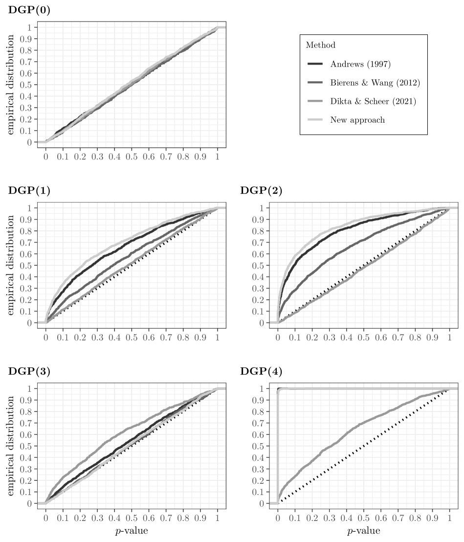
Figure 1: ECDF of bootstrap $p$-values for the simulated models

Clearly, all four methods behave appropriately in case the null hypothesis is fulfilled. Specifically, the $p$-values for DGP(0) are approximately uniformly distributed as the graphs are close to the dotted identity line. The plots corresponding to DGP(1) and DGP(2) indicate that our new approach is the most sensitive one to a violation of the distribution assumption. The likelihood of low $p$-values (corresponding to a rejection of $H_{0}$) is the highest for our method followed by Andrews’ and Bierens and Wang’s methods. The method studied by Dikta and Scheer, on the other hand, performs rather poorly in these examples as the $p$-value is approximately uniformly distributed. In the plot for DGP(3), however, it can be seen that Dikta and Scheer’s method seems to be the most sensitive one if the assumed linear relationship between $X$ and $Y$ is not valid. In this case, rejection is most likely using their method whereas the other methods fail to reject $H_{0}$. Finally, all methods except Dikta and Scheer’s react very senstively to a violation of the homoscedacity assumption as it is the case in DGP(4).

Bike sharing data

As a real-world dataset, we consider the bike sharing data from Fanaee-T (2013) that was also analyzed in Dikta & Scheer (2021). It contains the hourly and daily count of rental bikes in Washington DC in 2011 and 2012 together with corresponding weather and seasonal information. The data is preprocessed in the same way as discussed in Dikta & Scheer (2021, Example 5.44) leaving us with continuous variables for the normalized temperature, humidity and wind speed as well as factors indicating the weather situation, year, season and type of day (working day, holiday or day between Christmas and New Year).

As Dikta and Scheer, we use the daily rental counts as output variable $Y$ and all of the listed variables together with an intercept, the squared temperature, the squared humidity and an interaction term between year and season as covariate vector $X$. In section 6.1.2 of their book, Dikta and Scheer identify two parametric GLMs that seem to fit to the given data, i.e. that are not rejected by their goodness-of-fit test, namely a negative binomial and a log-transformed Gaussian model. In each model, the canonical link function is used: the logarithm for the negative binomial model and the identity function for the Gaussian model. The Gaussian model is called “log-transformed” as it uses $\log(Y)$ as response variable.

We want to investigate how well these two models fit to the given data according to our new approach using the conditional empirical process with estimated parameters. As illustrated in table 1, our new goodness-of-fit test results in an approximate $p$-value of zero for both parametric families, so they are clearly rejected. The method from Andrews (1997) and Bierens & Wang (2012) also yield very low $p$-values. In light of our previous simulation study, we could conclude that the regression function is probably correct (because Dikta and Scheer’s method accepts the models) but the distribution family is not chosen appropriately (because the other three methods reject the models). We fitted some more models using different distributions but could not find any that was not rejected by our new goodness-of-fit test.

Note that the high-dimensionality of the covariate vector $X$ results in a fairly long runtime for Andrew’s method. In particular, the calculation of the $p$-value took about 15 times longer than for our new approach and roughly 30 times longer than using Dikta and Scheer’s method.

Table 1: Bootstrap $p$-values of different tests and models fitted to the bike sharing data

Model	Andrews (1997)	Bierens & Wang (2012)	Dikta & Scheer (2021)	New approach
Log-transformed Gaussian	0.01	0.06	0.12	0
Negative binomial	0.03	0.01	0.08	0

Bank transaction data

As another real-world example, we use the bank transaction dataset from Fox & Weisberg (2018). It is composed of three variables: $t1$ and $t2$, the numbers of transactions of two types performed by $n=261$ branches of a large bank used as vector of covariates $X$, and time, the total time in minutes of labor in each branch used as response variable $Y$.

In a first step, we fit a classical linear model with normal distribution to the given data and compute the corresponding $p$-value according to the three different goodness-of-fit tests. The results are shown in table 2. The method introduced by Dikta & Scheer (2021) yields a $p$-value of $0.96$, so the model is clearly accepted. The goodness-of-fit tests from Andrews (1997) and Bierens & Wang (2012) as well as our new approach, however, reject the model with a $p$-value of $0$, $0.05$ and $0.06$, respectively. Recalling the results of the simulation study, such a combination is likely caused by a correct regression function but inappropriate distribution assumption in the model.

Table 2: Bootstrap $p$-values of different tests and models fitted to the bank transaction data

Model	Andrews (1997)	Bierens & Wang (2012)	Dikta & Scheer (2021)	New approach
Gaussian	0	0.05	0.96	0.06
Gamma	0.41	0.95	0.99	0.81

To come up with a more appropriate distribution family for $Y$ given $X$, we plotted the data and examined how the points are scattered around the mean. It could be seen that the variance of the data points does not seem to be constant as it would be the case in a Gaussian model. Instead, the data points are closer around the regression line for lower values of the conditional mean and more spread out for higher values. This behavior suggests a Gamma distribution implying a constant coefficient of variation.

So, in a next step, we fitted a linear model with Gamma distribution to the dataset and again used the three different tests to evaluate its goodness-of-fit. As illustrated in table 2, all of the methods yield high $p$-values this time meaning that the model is not rejected and thus seems to describe the data appropriately.

Appendix: Proofs

Proof of thm:conv_proc.

The proof will be based on a Durbin-like splitting of the process (see Durbin (1973)) given by

$$\tilde{\alpha}_{n}(t) =\underbrace{\frac{1}{\sqrt{n}}\sum_{i=1}^{n}{{I_{\left\{Y_{i}\leq t\right\}}}}-F(t|\vartheta_{0},X_{i})}_{\alpha_{n}^{(1)}(t)}$$

$$\quad+\underbrace{\frac{1}{\sqrt{n}}\sum_{i=1}^{n}F(t|\vartheta_{0},X_{i})-F(t|\hat{\vartheta}_{n},X_{i})}_{\alpha_{n}^{(2)}(t)}.$$

To prove the convergence of $\tilde{\alpha}_{n}$, we will first verify that the two processes are asymptotically tight in $\ell^{\infty}(\bar{\mathbb{R}})$ and find asymptotic iid representations for them to analyze the covariance structure of the finite-dimensional distributions (fidis). Then we use the multivariate central limit theorem (CLT) for the convergence of the fidis and finally apply Kosorok (2008, Theorem 7.17) to conclude the weak convergence of the process in $\ell^{\infty}(\bar{\mathbb{R}})$.

Asymptotic tightness of $\alpha_{n}^{(1)}$ will be shown by splitting it into two parts again:

$$\alpha_{n}^{(1)}(t) =\underbrace{\sqrt{n}\Big{(}F_{Y,n}(t)-F_{Y,0}(t)\Big{)}}_{\alpha_{n}^{(1a)}(t)}+\underbrace{\sqrt{n}\left(F_{Y,0}(t)-\frac{1}{n}\sum_{i=1}^{n}F(t|\vartheta_{0},X_{i})\right)}_{\alpha_{n}^{(1b)}(t)}.$$

The first summand $\alpha_{n}^{(1a)}$ represents the classical empirical process. It was proven to be a Donsker class by Donsker himself, see e.g. Kosorok (2008, p. 11). By Kosorok (2008, Lemma 7.12(ii)), it follows that $\alpha_{n}^{(1a)}$ is asymptotically tight in $\ell^{\infty}(\bar{\mathbb{R}})$.

To show asymptotic tightness of the second summand $\alpha_{n}^{(1b)}$, we write the process as

$$-\alpha_{n}^{(1b)}(t) =\sqrt{n}\left(\frac{1}{n}\sum_{i=1}^{n}F(t|\vartheta_{0},X_{i})-F_{Y,0}(t)\right)$$

$$=\sqrt{n}\left(\frac{1}{n}\sum_{i=1}^{n}F(t|\vartheta_{0},X_{i})-\mathbb{E}\left[F(t|\vartheta_{0},X)\right]\right).$$

This shows that $\alpha_{n}^{(1b)}$ can be regarded as a generalized empirical process over the index set $\tilde{\mathcal{F}}=\{x\mapsto F(t|\vartheta_{0},x)~{}|~{}t\in\mathbb{R}\}$. Now, we will use Kosorok (2008, Theorem 8.19) to show that $\tilde{\mathcal{F}}$ is a $\mathbb{P}$-Donsker class and consequently $\alpha_{n}^{(1b)}$ is asymptotically tight. An envelope function of $\tilde{\mathcal{F}}$ is given by $\tilde{F}(x)=1$ which is clearly square-integrable. As explained in the first paragraph on page 150 of Kosorok’s book, all measurability conditions of the theorem are satified if $\tilde{\mathcal{F}}$ is pointwise measurable. To see that this is in fact the case, define the countable set of functions $\tilde{\mathcal{G}}\coloneqq\{x\mapsto F(t|\vartheta_{0},x)~{}|~{}t\in\mathbb{Q}\}\subset\tilde{\mathcal{F}}$. Due to the right-continuity of $F(t|\vartheta_{0},x)$ in $t$, there exists a sequence $\{s_{m}\}\in\mathbb{Q}$ for every $t\in\mathbb{R}$ with $F(s_{m}|\vartheta_{0},x)\to F(t|\vartheta_{0},x)$ for every $x$. The final and main condition of Kosorok (2008, Theorem 8.19) is the boundedness of the uniform entropy integral. As noted at the beginning of page 158 in Kosorok’s book, it is satisfied if $\tilde{\mathcal{F}}$ is a VC-class of functions. This is true since $F(t|\vartheta_{0},x)$ is monotonically increasing in $t$ for every $x$, see Kosorok (2008, Lemma 9.10).

A linear representation of $\alpha_{n}^{(1)}$ is given by

$$\alpha_{n}^{(1)}(t)=n^{-1/2}\sum_{i=1}^{n}\xi^{(1)}(t,X_{i},Y_{i})$$

with

$$\xi^{(1)}(t,x,y) ={{I_{\left\{y\leq t\right\}}}}-F(t|\vartheta_{0},x)$$

$$\mathbb{E}_{\vartheta_{0}}\left[\xi^{(1)}(t,X,Y)\right] =0,$$

$$\text{COV}_{\vartheta_{0}}\left(\xi^{(1)}(s,X,Y),\xi^{(1)}(t,X,Y)\right) =\mathbb{P}_{\vartheta_{0}}\left(Y\leq\min(s,t)\right)-\mathbb{E}\left[F(s|\vartheta_{0},X)F(t|\vartheta_{0},X)\right]$$

Next, we want to examine $\alpha_{n}^{(2)}(t)$. Using ass:e1cond:mle_lin and the mean value theorem, we get

$$\alpha_{n}^{(2)}(t) =\frac{1}{\sqrt{n}}\sum_{i=1}^{n}F\big{(}t|\vartheta_{0},X_{i}\big{)}-F\big{(}t|\hat{\vartheta}_{n},X_{i}\big{)}$$

$$=-\sqrt{n}\left(\hat{\vartheta}_{n}-\vartheta_{0}\right)^{T}\frac{1}{n}\sum_{i=1}^{n}\frac{\partial}{\partial\vartheta}F(t|\tilde{\vartheta}_{n}(t,X_{i}),X_{i})$$

$$=-\left(n^{-1/2}\sum_{i=1}^{n}L^{T}(X_{i},Y_{i};\vartheta_{0})+o_{\mathbb{P}}(1)\right)\left(\frac{1}{n}\sum_{i=1}^{n}w(t,\tilde{\vartheta}_{n}(t,X_{i}),X_{i})\right)$$

with $\tilde{\vartheta}_{n}(t,X_{i})$ lying on the line segment between $\vartheta_{0}$ and $\hat{\vartheta}_{n}$ dependent on $t$ and $X_{i}$. Next, we would like to replace the second factor by $W(t,\vartheta_{0})$. Let $\varepsilon>0$. We have, by Markov’s inequality, for any $k=1,\dots,q$ and $\delta>0$ that

$$\mathbb{P}\left(\sup_{t\in\bar{\mathbb{R}}}\absolutevalue{\frac{1}{n}\sum_{i=1}^{n}w_{k}(t,\tilde{\vartheta}_{n}(t,X_{i}),X_{i})-w_{k}(t,\vartheta_{0},X_{i})}>\varepsilon\right)$$

$$\quad\leq\mathbb{P}\left(\frac{1}{n}\sum_{i=1}^{n}\sup_{\norm{\vartheta-\vartheta_{0}}<\delta}\sup_{t\in\bar{\mathbb{R}}}\absolutevalue{w_{k}(t,\vartheta,X_{i})-w_{k}(t,\vartheta_{0},X_{i})}>\varepsilon\right)+\mathbb{P}\left(\norm{\hat{\vartheta}_{n}-\vartheta_{0}}>\delta\right)$$

$$\quad\leq\frac{1}{\varepsilon}\cdot\mathbb{E}\left[\sup_{\norm{\vartheta-\vartheta_{0}}<\delta}\sup_{t\in\bar{\mathbb{R}}}\absolutevalue{w_{k}(t,\vartheta,X)-w_{k}(t,\vartheta_{0},X)}\right]+\mathbb{P}\left(\norm{\hat{\vartheta}_{n}-\vartheta_{0}}>\delta\right).$$

By ass:e1cond:mle_lin, the second summand vanishes as $n$ tends to infinity. Furthermore, by ass:m2cond:w_cont, the integrand of the first summand goes to zero as $\delta$ tends to zero and due to ass:m1cond:v_ddom, we can apply Lebesgue’s dominated convergence theorem (DCT) to follow that the whole term converges to zero. For that, note that because of ass:m1cond:v_ex_dom, the order of integration and differentiation can be interchanged and we have

$$\absolutevalue{w_{k}(t,\vartheta,x)} =\absolutevalue{\int_{-\infty}^{t}v_{k}(s,\vartheta,x)\nu(ds)}$$

$$\leq\int_{-\infty}^{t}\absolutevalue{v_{k}(s,\vartheta,x)}\nu(ds)$$

$$\leq\sup_{\tilde{\vartheta}\in V}\int\absolutevalue{v_{k}(s,\tilde{\vartheta},x)}\nu(ds),$$

which is integrable according to ass:m1cond:v_ddom. Further, we have for any $K>0$

$$\sup_{t\in\bar{\mathbb{R}}}\absolutevalue{\frac{1}{n}\sum_{i=1}^{n}w_{k}(t,\vartheta_{0},X_{i})-W(t,\vartheta_{0})}$$

$$\quad=\sup_{t\in\bar{\mathbb{R}}}\absolutevalue{\int w_{k}(t,\vartheta_{0},x)(H_{n}-H)(dx)}$$

$$\quad=\sup_{t\in\bar{\mathbb{R}}}\absolutevalue{\int\int_{-\infty}^{t}v_{k}(s,\vartheta_{0},x)\nu(ds)(H_{n}-H)(dx)}$$

$$\quad\leq\sup_{|t|\leq K}\absolutevalue{\int\int_{-K}^{t}v_{k}(s,\vartheta_{0},x)\nu(ds)(H_{n}-H)(dx)}$$

$$\qquad+\int\int{{I_{\left\{|s|>K\right\}}}}\absolutevalue{v_{k}(s,\vartheta_{0},x)}\nu(ds)H_{n}(dx)+\int\int{{I_{\left\{|s|>K\right\}}}}\absolutevalue{v_{k}(s,\vartheta_{0},x)}\nu(ds)H(dx)$$

$$\quad\eqqcolon A_{1,n}(K)+A_{2,n}(K)+A_{3}(K).$$

By Jennrich (1969, Theorem 2), applicable due to ass:m1, $A_{1,n}(K)$ converges to zero as $n$ goes to infinity for any value of $K$. Moreover, an iterated application of Lebesgue’s DCT using ass:m1 to find dominating integrable functions, yields

$$\lim_{K\to\infty}A_{3}(K)=\int\int\lim_{K\to\infty}{{I_{\left\{|s|>K\right\}}}}\absolutevalue{v_{k}(s,\vartheta_{0},x)}\nu(ds)H(dx)=0.$$

Since, by SLLN, $\lim_{n\to\infty}A_{2,n}(K)=A_{3}(K)$ wp1, the second term also vanishes as $n$ and $K$ tend to infinity. So we can follow that

$$\sup_{t\in\bar{\mathbb{R}}}\norm{\frac{1}{n}\sum_{i=1}^{n}w(t,\tilde{\vartheta}_{n}(t,X_{i}),X_{i})-W(t,\vartheta_{0})}=o_{\mathbb{P}}(1).$$

Altogether, we get

$$\alpha_{n}^{(2)}(t)=n^{-1/2}\sum_{i=1}^{n}\xi^{(2)}(t,X_{i},Y_{i})+r^{(2)}_{n}(t)$$

with

$$\xi^{(2)}(t,x,y) =-\left(L(x,y;\vartheta_{0})\right)^{T}W(t,\vartheta_{0})$$

$$\mathbb{E}_{\vartheta_{0}}\left[\xi^{(2)}(t,X,Y)\right] =0,$$

$$\text{COV}_{\vartheta_{0}}\left(\xi^{(2)}(s,X,Y),\xi^{(2)}(t,X,Y)\right) =W^{T}(s,\vartheta_{0})\text{COV}_{\vartheta_{0}}\left(L(X,Y;\vartheta_{0})\right)W(t,\vartheta_{0})$$

$$r^{(2)}_{n}(t) \to 0\text{ a.s.\ uniformly in }t.$$

To prove the tightness of $\alpha_{n}^{(2)}(t)$, note that $L$ is not dependent on $t$ and $W(t,\vartheta_{0})$ is continuous in $t$ by assumption ass:m2cond:W_cont. Thus, the process is in $C[-\infty,\infty]$ and we can use Billingsley (1968, Theorem 8.2) to verify tightness. By the multivariate CLT, there is a centered normal random vector $S_{\infty}$ such that $S_{n}=-n^{-1/2}\sum_{i=1}^{n}L(X_{i},Y_{i};\vartheta_{0})\Rightarrow S_{\infty}$. Since $W(0,\vartheta_{0})$ is a deterministic vector, $\alpha_{n}^{(2)}(0)=S_{n}^{T}W(0,\vartheta_{0})+r_{n}(0)$ converges as well and is thus tight in $\mathbb{R}$ by Prokhorov’s Theorem. It remains to show that for every $\varepsilon,\eta>0$, there exists a $\delta>0$ and $n_{0}\in\mathbb{N}$ such that for all $n\geq n_{0}$

$$\mathbb{P}\left(\sup_{\absolutevalue{s-t}<\delta}\absolutevalue{\alpha_{n}^{(2)}(s)-\alpha_{n}^{(2)}(t)}\geq\varepsilon\right)\leq\eta.$$ (3)

For any $\varepsilon,\eta>0$, we have

$$\mathbb{P}\left(\sup_{\absolutevalue{s-t}<\delta}\absolutevalue{\alpha_{n}^{(2)}(s)-\alpha_{n}^{(2)}(t)}\geq\varepsilon\right)$$

$$\quad=\mathbb{P}\left(\sup_{\absolutevalue{s-t}<\delta}\absolutevalue{S_{n}^{T}\Big{(}W(s,\vartheta_{0})-W(t,\vartheta_{0})\Big{)}+r_{n}(s)-r_{n}(t)}\geq\varepsilon\right)$$

$$\quad\leq\mathbb{P}\left(\norm{S_{n}}\sup_{\absolutevalue{s-t}<\delta}\norm{\left(W(s,\vartheta_{0})-W(t,\vartheta_{0})\right)}\geq\frac{\varepsilon}{3}\right)+2\cdot\mathbb{P}\left(\sup_{t\in\mathbb{R}}\absolutevalue{r_{n}(t)}\geq\frac{\varepsilon}{3}\right)$$

$$=\mathbb{P}\left(\norm{S_{n}}\geq\frac{\varepsilon}{3\cdot\sup_{\absolutevalue{s-t}<\delta}\norm{\left(W(s,\vartheta_{0})-W(t,\vartheta_{0})\right)}}\right)+2\cdot\mathbb{P}\left(\sup_{t\in\mathbb{R}}\absolutevalue{r_{n}(t)}\geq\frac{\varepsilon}{3}\right).$$

The second summand clearly converges to zero as $n$ goes to infinity. For the first summand, choose $c_{\infty}$ such that $\mathbb{P}\left(\norm{S_{\infty}}\geq c_{\infty}\right)\leq\frac{\eta}{2}$ and $n_{0}\in\mathbb{N}$ such that for all $n\geq n_{0}$

$$\mathbb{P}\left(\norm{S_{n}}\geq c_{\infty}\right) \leq\absolutevalue{\mathbb{P}\left(\norm{S_{n}}\geq c_{\infty}\right)-\mathbb{P}\left(\norm{S_{\infty}}\geq c_{\infty}\right)}+\mathbb{P}\left(\norm{S_{\infty}}\geq c_{\infty}\right)$$

$$\leq\frac{\eta}{2}+\frac{\eta}{2}=\eta.$$

Since $W(t,\vartheta_{0})$ is uniformly continuous in $t$, we can find a $\delta$ such that

$$\frac{\varepsilon}{3\cdot\sup_{\absolutevalue{s-t}<\delta}\norm{\left(W(s,\vartheta_{0})-W(t,\vartheta_{0})\right)}}\geq c_{\infty},$$

which concludes the proof of (3). Note that uniform tightness in $C[-\infty,\infty]$ implies uniform tightness in the larger space $\ell^{\infty}(\bar{\mathbb{R}})$ which in turn implies asymptotic tightness in $\ell^{\infty}(\bar{\mathbb{R}})$.

Due to their asymptotic linear representations, the fidis of $\alpha_{n}^{(1)}$ and $\alpha_{n}^{(2)}$ converge to a centered normal distribution by the multivariate CLT. Having established their asymptotic tightness as well, we can apply Kosorok (2008, Theorem 7.17) to follow that both processes and thus also their sum $\tilde{\alpha}_{n}$ converges weakly to a centered Gaussian process in $\ell^{\infty}(\bar{\mathbb{R}})$. The only step left to prove the statement of the theorem is the calculation of the covariance structure of the limiting process. The auto-covariance functions of $\alpha_{n}^{(1)}(t)$ and $\alpha_{n}^{(2)}(t)$ are already given above. For their cross-covariance function, we get

$$\text{COV}_{\vartheta_{0}}\left(\xi^{(1)}(s,X,Y),\xi^{(2)}(t,X,Y)\right)$$

$$\quad=\mathbb{E}_{\vartheta_{0}}\left[\quantity({{I_{\left\{Y\leq s\right\}}}}-F(s|\vartheta_{0},X))\quantity(-L^{T}(X,Y;\vartheta_{0})W(t,\vartheta_{0}))\right]$$

$$\quad=W^{T}(t,\vartheta_{0})\mathbb{E}_{\vartheta_{0}}\left[\quantity(F(s|\vartheta_{0},X)-{{I_{\left\{Y\leq s\right\}}}})L(X,Y;\vartheta_{0})\right].\qed$$

Proof of thm:conv_proc_boot.

The proof is similar to the proof of convergence of the original test statistic. We start by splitting the process as follows

$$\tilde{\alpha}_{n}^{*}(t) =\underbrace{\frac{1}{\sqrt{n}}\sum_{i=1}^{n}{{I_{\left\{Y_{i,n}^{*}\leq t\right\}}}}-F(t|\hat{\vartheta}_{n},X_{i})}_{\alpha_{n}^{(1*)}(t)}$$

$$\quad+\underbrace{\frac{1}{\sqrt{n}}\sum_{i=1}^{n}F(t|\hat{\vartheta}_{n},X_{i})-F(t|\hat{\vartheta}_{n}^{*},X_{i})}_{\alpha_{n}^{(2*)}(t)}.$$

To prove the convergence of $\tilde{\alpha}_{n}^{*}$, we will again apply Kosorok (2008, Theorem 7.17). We start by proving the convergence of $\alpha_{n}^{(1*)}$ using Kosorok (2008, Theorem 11.16). Since the $X_{i}$ are fixed under $\mathbb{P}_{n}^{*}$, we can write

$$\alpha_{n}^{(1*)}(t) =\frac{1}{\sqrt{n}}\sum_{i=1}^{n}{{I_{\left\{Y_{i,n}^{*}\leq t\right\}}}}-F(t|\hat{\vartheta}_{n},X_{i})$$

$$=\sum_{i=1}^{n}\tilde{f}_{n,i}(t)-\mathbb{E}_{n}^{*}\left[\tilde{f}_{n,i}(t)\right],$$

where $\tilde{f}_{n,i}(t)=\frac{1}{\sqrt{n}}{{I_{\left\{Y_{i,n}^{*}\leq t\right\}}}}$ with envelope $\tilde{F}_{n,i}=\frac{1}{\sqrt{n}}$. The separability of $\{\tilde{f}_{n,i}\}$ can be shown with a similar argument as in the original convergence proof using the fact that $\tilde{f}_{n,i}(t)$ is right-continuous. By Kosorok (2008, Lemma 11.15), it follows that the triangular array is almost measurable Suslin. The manageability condition (A) of Kosorok (2008, Theorem 11.16) is fulfilled since the indicator functions in $\tilde{f}_{n,i}(t)$ are monotone increasing in $t$ (see page 221 in Kosorok’s book). The second condition (B) holds as

$$\tilde{K}(s,t) \coloneqq\lim_{n\to\infty}\mathbb{E}_{n}^{*}\left[\alpha_{n}^{(1*)}(s)\alpha_{n}^{(1*)}(t)\right]$$

$$=\lim_{n\to\infty}\frac{1}{n}\mathbb{E}_{n}^{*}\left[\sum_{i=1}^{n}\sum_{j=1}^{n}\left({{I_{\left\{Y_{i,n}^{*}\leq s\right\}}}}-F(s|\hat{\vartheta}_{n},X_{i})\right)\left({{I_{\left\{Y_{j,n}^{*}\leq t\right\}}}}-F(t|\hat{\vartheta}_{n},X_{j})\right)\right]$$

$$=_{(1)}\lim_{n\to\infty}\frac{1}{n}\sum_{i=1}^{n}\mathbb{E}_{n}^{*}\left[\left({{I_{\left\{Y_{i,n}^{*}\leq s\right\}}}}-F(s|\hat{\vartheta}_{n},X_{i})\right)\left({{I_{\left\{Y_{i,n}^{*}\leq t\right\}}}}-F(t|\hat{\vartheta}_{n},X_{i})\right)\right]$$

$$=_{(2)}\mathbb{E}_{\vartheta_{0}}\left[\left({{I_{\left\{Y\leq s\right\}}}}-F(s|\vartheta_{0},X)\right)\left({{I_{\left\{Y\leq t\right\}}}}-F(t|\vartheta_{0},X)\right)\right]$$

$$=\mathbb{P}_{\vartheta_{0}}\left(Y\leq\min(s,t)\right)-\mathbb{E}\left[F(s|\vartheta_{0},X)F(t|\vartheta_{0},X)\right]<\infty,$$

where for the equality $=_{(1)}$, we used the fact that $Y_{1,n}^{*},\dots,Y_{n,n}^{*}$ are independent, and in $=_{(2)}$, we applied Dikta & Scheer (2021, Lemma 5.58). Note that the lemma is applicable due to ass:m3. The verification of the next two conditions, (C) and (D), is straightforward:

$$\limsup_{n\to\infty}\sum_{i=1}^{n}\mathbb{E}_{n}^{*}\left[\tilde{F}_{n,i}^{2}\right]=\limsup_{n\to\infty}\sum_{i=1}^{n}\frac{1}{n}=1<\infty$$

and

$$\sum_{i=1}^{n}\mathbb{E}_{n}^{*}\left[\tilde{F}_{n,i}{{I_{\left\{\tilde{F}_{n,i}>\varepsilon\right\}}}}\right]=\sum_{i=1}^{n}\mathbb{E}_{n}^{*}\left[\frac{1}{n}{{I_{\left\{\frac{1}{\sqrt{n}}>\varepsilon\right\}}}}\right]={{I_{\left\{\frac{1}{\sqrt{n}}>\varepsilon\right\}}}}\xrightarrow[n\to\infty]{}0\quad\forall\varepsilon>0.$$

For condition (E), we need to consider $\rho_{n}(s,t)\coloneqq\quantity(\sum_{i=1}^{n}\mathbb{E}_{n}^{*}\left[\absolutevalue{\tilde{f}_{n,i}(s)-\tilde{f}_{n,i}(t)}^{2}\right])^{\frac{1}{2}}$. By ass:m3 and Dikta & Scheer (2021, Lemma 5.58), we have

$$\rho_{n}(s,t) =\quantity(\frac{1}{n}\sum_{i=1}^{n}\mathbb{E}_{n}^{*}\left[\absolutevalue{{{I_{\left\{Y_{i,n}^{*}\leq s\right\}}}}-{{I_{\left\{Y_{i,n}^{*}\leq t\right\}}}}}\right])^{\frac{1}{2}}$$

$$\xrightarrow[n\to\infty]{}\quantity(\mathbb{E}_{\vartheta_{0}}\left[\absolutevalue{{{I_{\left\{Y\leq s\right\}}}}-{{I_{\left\{Y\leq t\right\}}}}}\right])^{\frac{1}{2}}\eqqcolon\rho(s,t).$$

Assume that $\{s_{n}\},\{t_{n}\}\in\mathbb{R}$ with $\rho(s_{n},t_{n})\to 0$. Then we have

$$\rho_{n}(s_{n},t_{n}) \leq\sup_{s,t\in\bar{\mathbb{R}}}\absolutevalue{\rho_{n}(s,t)-\rho(s,t)}+\rho(s_{n},t_{n}).$$

The second summand converges to zero by assumption. Since, similarly to the reverse triangle inequality, it holds $\sqrt{|a-b|}\geq\absolutevalue{\sqrt{a}-\sqrt{b}}$, we get for the first summand

$$\sup_{s,t\in\bar{\mathbb{R}}}\absolutevalue{\rho_{n}(s,t)-\rho(s,t)}^{2}$$

$$\quad=\sup_{s,t\in\bar{\mathbb{R}}}\absolutevalue{\quantity(\frac{1}{n}\sum_{i=1}^{n}\mathbb{E}_{n}^{*}\left[\absolutevalue{{{I_{\left\{Y_{i,n}^{*}\leq s\right\}}}}-{{I_{\left\{Y_{i,n}^{*}\leq t\right\}}}}}\right])^{\frac{1}{2}}-\quantity(\mathbb{E}_{\vartheta_{0}}\left[\absolutevalue{{{I_{\left\{Y\leq s\right\}}}}-{{I_{\left\{Y\leq t\right\}}}}}\right])^{\frac{1}{2}}}^{2}$$

$$\quad\leq\sup_{s,t\in\bar{\mathbb{R}}}\absolutevalue{\frac{1}{n}\sum_{i=1}^{n}\mathbb{E}_{n}^{*}\left[\absolutevalue{{{I_{\left\{Y_{i,n}^{*}\leq s\right\}}}}-{{I_{\left\{Y_{i,n}^{*}\leq t\right\}}}}}\right]-\mathbb{E}_{\vartheta_{0}}\left[\absolutevalue{{{I_{\left\{Y\leq s\right\}}}}-{{I_{\left\{Y\leq t\right\}}}}}\right]}.$$

Several applications of the triangle inequality further yield

$$\sup_{s,t\in\bar{\mathbb{R}}}\absolutevalue{\rho_{n}(s,t)-\rho(s,t)}^{2}$$

$$\quad\leq\sup_{s,t\in\bar{\mathbb{R}}}\absolutevalue{\frac{1}{n}\sum_{i=1}^{n}\mathbb{E}_{n}^{*}\left[{{I_{\left\{Y_{i,n}^{*}\leq s\right\}}}}+{{I_{\left\{Y_{i,n}^{*}\leq t\right\}}}}\right]-\mathbb{E}_{\vartheta_{0}}\left[{{I_{\left\{Y\leq s\right\}}}}+{{I_{\left\{Y\leq t\right\}}}}\right]}$$

$$\quad=2\sup_{t\in\bar{\mathbb{R}}}\absolutevalue{\frac{1}{n}\sum_{i=1}^{n}\mathbb{E}_{n}^{*}\left[{{I_{\left\{Y_{i,n}^{*}\leq t\right\}}}}\right]-\mathbb{E}_{\vartheta_{0}}\left[{{I_{\left\{Y\leq t\right\}}}}\right]}$$

$$\quad=2\sup_{t\in\bar{\mathbb{R}}}\absolutevalue{\mathbb{E}\left[F(t|\vartheta_{0},X)\right]-\frac{1}{n}\sum_{i=1}^{n}F(t|\hat{\vartheta}_{n},X_{i})}$$

$$\quad\leq 2\left(\sup_{t\in\bar{\mathbb{R}}}\absolutevalue{\mathbb{E}\left[F(t|\vartheta_{0},X)\right]-\frac{1}{n}\sum_{i=1}^{n}F(t|\vartheta_{0},X_{i})}+\sup_{t\in\bar{\mathbb{R}}}\absolutevalue{\frac{1}{n}\sum_{i=1}^{n}F(t|\vartheta_{0},X_{i})-F(t|\hat{\vartheta}_{n},X_{i})}\right).$$

The almost sure convergence of the first summand to zero is equivalent to saying that $\tilde{\mathcal{F}}=\{x\mapsto F(t|\vartheta_{0},x)~{}|~{}t\in\mathbb{R}\}$ is a Glivenko-Cantelli class. This is in fact the case as we showed $\tilde{\mathcal{F}}$ to be Donsker in the proof of thm:conv_proc and every Donsker class is also Glivenko-Cantelli (see Kosorok (2008, Lemma 8.17)). To analyze the convergence of the second summand, we use a Taylor expansion and the Cauchy-Schwarz inequality yielding

$$\sup_{t\in\bar{\mathbb{R}}}\absolutevalue{\frac{1}{n}\sum_{i=1}^{n}F(t|\vartheta_{0},X_{i})-F(t|\hat{\vartheta}_{n},X_{i})}$$

$$\quad=\sup_{t\in\mathbb{R}}\absolutevalue{\quantity(\hat{\vartheta}_{n}-\vartheta_{0})^{T}\frac{1}{n}\sum_{i=1}^{n}w(t,\tilde{\vartheta}_{n}(t,X_{i}),X_{i})}$$

$$\quad\leq\norm{\hat{\vartheta}_{n}-\vartheta_{0}}\sup_{t\in\mathbb{R}}\norm{\frac{1}{n}\sum_{i=1}^{n}w(t,\tilde{\vartheta}_{n}(t,X_{i}),X_{i})},$$ (4)

where $\tilde{\vartheta}_{n}(t,X_{i})$ lies on the line segment connecting $\vartheta_{0}$ and $\hat{\vartheta}_{n}$ and depends on $t$ and $X_{i}$. By ass:e1cond:mle_conv_wp1, $\norm{\hat{\vartheta}_{n}-\vartheta_{0}}$ converges to zero wp1 as $n$ goes to infinity. So the desired result follows if the supremum term is appropriately bounded. Since $\hat{\vartheta}_{n}$ converges almost surely to $\vartheta_{0}$, $\tilde{\vartheta}_{n}(t,X_{i})$ will eventually lie in $V$. We have

$$\sup_{\vartheta\in V}\sup_{t\in\mathbb{R}}\norm{w(t,\vartheta,x)} =\sup_{\vartheta\in V}\sup_{t\in\mathbb{R}}\norm{\int_{-\infty}^{t}v(s,\vartheta,x)\nu(ds)}$$

$$\leq\sup_{\vartheta\in V}\int_{-\infty}^{\infty}\norm{v(s,\vartheta,x)}\nu(ds)$$

$$\eqqcolon M_{w}(x),$$

which is an H-integrable function according to ass:m1cond:v_ddom. It follows that (for sufficiently large $n$)

$$\sup_{t\in\mathbb{R}}\norm{\frac{1}{n}\sum_{i=1}^{n}w(t,\tilde{\vartheta}_{n}(t,X_{i}),X_{i})} \leq\sup_{\vartheta\in V}\sup_{t\in\mathbb{R}}\norm{\frac{1}{n}\sum_{i=1}^{n}w(t,\vartheta,X_{i})}$$

$$\leq\frac{1}{n}\sum_{i=1}^{n}\sup_{\vartheta\in V}\sup_{t\in\mathbb{R}}\norm{w(t,\vartheta,X_{i})}$$

$$\leq\frac{1}{n}\sum_{i=1}^{n}M_{w}(X_{i}).$$

By the SLLN, the arithmetic mean converges to the finite expected value $\mathbb{E}\left[M_{w}(X)\right]=\int M_{w}(x)H(dx)$. It follows that the product on the right-hand side of (4) converges to zero wp1. In summary, we have verified all five conditions (A)-(E) of Kosorok (2008, Theorem 11.16) and hence can conclude that $\alpha_{n}^{(1*)}$ converges to a tight centered Gaussian process with auto-covariance function $\tilde{K}(s,t)$. By Kosorok (2008, Lemma 7.12), it follows that $\alpha_{n}^{(1*)}$ is asymptotically tight.

Next, we investigate $\alpha_{n}^{(2*)}$. In particular, we will find an asymptotically equivalent representation. Using a Taylor expansion and ass:e2cond:mle_lin_boot, we have

$$\alpha_{n}^{(2*)}(t) =\frac{1}{\sqrt{n}}\sum_{i=1}^{n}F(t|\hat{\vartheta}_{n},X_{i})-F(t|\hat{\vartheta}_{n}^{*},X_{i})$$

$$=-\sqrt{n}\quantity(\hat{\vartheta}_{n}^{*}-\hat{\vartheta}_{n})^{T}\frac{1}{n}\sum_{i=1}^{n}\frac{\partial}{\partial\vartheta}F(t|\tilde{\vartheta}_{n}^{*}(t,X_{i}),X_{i})$$

$$=-\quantity(n^{-1/2}\sum_{i=1}^{n}L^{T}(X_{i},Y_{i,n}^{*},\hat{\vartheta}_{n})+o_{\mathbb{P}_{n}^{*}}(1))\frac{1}{n}\sum_{i=1}^{n}w(t,\tilde{\vartheta}_{n}^{*}(t,X_{i}),X_{i}),$$

where $\tilde{\vartheta}_{n}^{*}(t,X_{i})$ lies on the line segment connecting $\hat{\vartheta}_{n}$ and $\hat{\vartheta}_{n}^{*}$ and may depend on $t$ and $X_{i}$. We can estimate

$$\mathbb{P}_{n}^{*}\quantity(\sup_{t\in\bar{\mathbb{R}}}\absolutevalue{\frac{1}{n}\sum_{i=1}^{n}w_{k}(t,\tilde{\vartheta}_{n}^{*}(t,X_{i}),X_{i})-w_{k}(t,\vartheta_{0},X_{i})}>\varepsilon)$$

$$\quad\leq\mathbb{P}_{n}^{*}\quantity(\sup_{\norm{\vartheta-\vartheta_{0}}<\delta}\sup_{t\in\bar{\mathbb{R}}}\absolutevalue{\frac{1}{n}\sum_{i=1}^{n}w_{k}(t,\vartheta,X_{i})-w_{k}(t,\vartheta_{0},X_{i})}>\varepsilon)+\mathbb{P}_{n}^{*}\quantity(\norm{\hat{\vartheta}_{n}^{*}-\vartheta_{0}}>\delta).$$

As $\norm{\hat{\vartheta}_{n}^{*}-\hat{\vartheta}_{n}}=o_{\mathbb{P}_{n}^{*}}(1)$ and $\norm{\hat{\vartheta}_{n}-\vartheta_{0}}\to 0$ wp1 by ass:e1cond:mle_conv_wp1 and E2cond:mle_lin_boot, it follows that the second term on the right-hand side converges to zero as $n$ goes to infinity. The argument of the first summand does not involve any randomness with respect to $\mathbb{P}_{n}^{*}$, so we consider

$$\limsup_{n\to\infty}\sup_{\norm{\vartheta-\vartheta_{0}}<\delta}\sup_{t\in\bar{\mathbb{R}}}\absolutevalue{\frac{1}{n}\sum_{i=1}^{n}w_{k}(t,\vartheta,X_{i})-w_{k}(t,\vartheta_{0},X_{i})}$$

$$\quad\leq\limsup_{n\to\infty}\frac{1}{n}\sum_{i=1}^{n}\sup_{\norm{\vartheta-\vartheta_{0}}<\delta}\sup_{t\in\bar{\mathbb{R}}}\absolutevalue{w_{k}(t,\vartheta,X_{i})-w_{k}(t,\vartheta_{0},X_{i})}$$

$$\quad=\mathbb{E}\left[\sup_{\norm{\vartheta-\vartheta_{0}}<\delta}\sup_{t\in\bar{\mathbb{R}}}\absolutevalue{w_{k}(t,\vartheta,X)-w_{k}(t,\vartheta_{0},X)}\right],$$

where the last equality follows from the SLLN together with the integrability condition for $w_{k}$. By Lebesgue’s DCT applicable due to ass:m1 and ass:m2cond:w_cont, the resulting expected value vanishes as $\delta$ tends to zero. As proven in thm:conv_proc, we have wp1

$$\sup_{t\in\bar{\mathbb{R}}}\norm{\frac{1}{n}\sum_{i=1}^{n}w(t,\vartheta_{0},X_{i})-W(t,\vartheta_{0})}\to 0\quad\text{as }n\to\infty.$$

It follows that wp1

$$\sup_{t\in\bar{\mathbb{R}}}\norm{\frac{1}{n}\sum_{i=1}^{n}w(t,\tilde{\vartheta}_{n}^{*}(t,X_{i}),X_{i})-W(t,\vartheta_{0})}=o_{\mathbb{P}_{n}^{*}}(1).$$

Altogether, we get wp1

$$\alpha_{n}^{(2*)}(t)=n^{-1/2}\sum_{i=1}^{n}W^{T}(t,\vartheta_{0})L(X_{i},Y_{i,n}^{*},\hat{\vartheta}_{n})+o_{\mathbb{P}_{n}^{*}}(1)$$

uniformly in $t$. Since the sum on the right hand side is asymptotically equivalent to $\alpha_{n}^{(2*)}(t)$ in the sense of Billingsley (1968, Theorem 4.1), we will substitute it from now on without mentioning it again.

To analyze the convergence of the fidis of $\tilde{\alpha}_{n}^{*}$ we use Cramér-Wold device (see e.g. Billingsley (1968, Theorem 7.7)). So we need to show that

$$\forall k\in\mathbb{N},~{}(t_{1},\dots,t_{k})\in\mathbb{R}^{k},~{}0\neq a\in\mathbb{R}^{k}:\quad\sum_{j=1}^{k}a_{j}\tilde{\alpha}_{n}^{*}(t_{j})\Rightarrow\mathcal{N}(0,a^{t}\Sigma a)\quad\text{wp1},$$ (5)

where $\Sigma_{j,l}=K(t_{j},t_{l})$ for $1\leq j,l\leq k$. We have

$$Z_{n}^{*} =\sum_{j=1}^{k}a_{j}\tilde{\alpha}_{n}^{*}(t_{j})$$

$$=\sum_{i=1}^{n}\underbrace{\sum_{j=1}^{k}a_{j}\frac{1}{\sqrt{n}}\quantity({{I_{\left\{Y_{i,n}^{*}\leq t_{j}\right\}}}}-F(t_{j}|\hat{\vartheta}_{n},X_{i}))}_{\xi_{i,n}^{*}}-\underbrace{\sum_{j=1}^{k}a_{j}W^{T}(t_{j},\vartheta_{0})}_{A^{T}}\underbrace{\frac{1}{\sqrt{n}}L(X_{i},Y_{i,n}^{*},\hat{\vartheta}_{n})}_{\eta_{i,n}^{*}}$$

with $\mathbb{E}_{n}^{*}\left[\xi_{i,n}^{*}\right]=\mathbb{E}_{n}^{*}\left[\eta_{i,n}^{*}\right]=0$ and $(\xi_{1,n}^{*},\eta_{1,n}^{*}),\dots,(\xi_{n,n}^{*},\eta_{n,n}^{*})$ independent. It follows that

$$\text{Var}_{n}^{*}\left(Z_{n}^{*}\right) =\sum_{i=1}^{n}\text{Var}_{n}^{*}\left(\xi_{i,n}^{*}\right)+\text{Var}_{n}^{*}\left(A^{T}\eta_{i,n}^{*}\right)-2\text{COV}_{n}^{*}\left(\xi_{i,n}^{*},A^{T}\eta_{i,n}^{*}\right)$$

$$=\sum_{i=1}^{n}\mathbb{E}_{n}^{*}\left[\xi_{i,n}^{*2}\right]+A^{T}\mathbb{E}\left[\eta_{i,n}^{*}\eta_{i,n}^{*T}\right]A-2A^{T}\mathbb{E}_{n}^{*}\left[\xi_{i,n}^{*}\eta_{i,n}^{*}\right].$$

For the first summand, we get

$$\sum_{i=1}^{n}\mathbb{E}_{n}^{*}\left[\xi_{i,n}^{*2}\right]$$

$$\quad=\frac{1}{n}\sum_{i=1}^{n}\sum_{j=1}^{k}\sum_{l=1}^{k}a_{j}a_{l}\mathbb{E}_{n}^{*}\left[\quantity({{I_{\left\{Y_{i,n}^{*}\leq t_{j}\right\}}}}-F(t_{j}|\hat{\vartheta}_{n},X_{i}))\quantity({{I_{\left\{Y_{i,n}^{*}\leq t_{l}\right\}}}}-F(t_{l}|\hat{\vartheta}_{n},X_{i}))\right]$$

$$\quad=\sum_{j=1}^{k}\sum_{l=1}^{k}a_{j}\quantity(\frac{1}{n}\sum_{i=1}^{n}\mathbb{E}_{n}^{*}\left[{{I_{\left\{Y_{i,n}^{*}\leq\min(t_{j},t_{l})\right\}}}}\right]-F(t_{j}|\hat{\vartheta}_{n},X_{i})F(t_{l}|\hat{\vartheta}_{n},X_{i}))a_{l}$$

$$\quad\xrightarrow[n\to\infty]{}\sum_{j=1}^{k}\sum_{l=1}^{k}a_{j}\Big{(}\mathbb{E}_{\vartheta_{0}}\left[{{I_{\left\{Y\leq\min(t_{j},t_{l})\right\}}}}\right]-\mathbb{E}\left[F(t_{j}|\vartheta_{0},X)F(t_{l}|\vartheta_{0},X)\right]\Big{)}a_{l}$$

$$\quad=\sum_{j=1}^{k}\sum_{l=1}^{k}a_{j}\tilde{K}(t_{j},t_{l})a_{l},$$

using Dikta & Scheer (2021, Lemma 5.58) for the convergence, applicable due to ass:m3. By ass:e2(ii), the second summand converges as well:

$$\sum_{i=1}^{n}A^{T}\mathbb{E}_{n}^{*}\left[\eta_{i,n}^{*}\eta_{i,n}^{*T}\right]A =A^{T}\frac{1}{n}\sum_{i=1}^{n}\mathbb{E}_{n}^{*}\left[L(X_{i},Y_{i,n}^{*},\hat{\vartheta}_{n})L^{T}(X_{i},Y_{i,n}^{*},\hat{\vartheta}_{n})\right]A$$

$$\xrightarrow[n\to\infty]{}A^{T}\mathbb{E}_{\vartheta_{0}}\left[L(X,Y,\vartheta_{0})L^{T}(X,Y,\vartheta_{0})\right]A$$

$$=\sum_{j=1}^{k}\sum_{l=1}^{k}a_{j}W^{T}(t_{j},\vartheta_{0})\text{COV}_{\vartheta_{0}}\left(L(X,Y,\vartheta_{0})\right)W(t_{l},\vartheta_{0})a_{l}.$$

Finally, another application of Dikta & Scheer (2021, Lemma 5.58) using ass:e3cond:xi_cont_int yields

$$\sum_{i=1}^{n}A^{T}\mathbb{E}_{n}^{*}\left[\xi_{i,n}^{*}\eta_{i,n}^{*}\right]$$

$$\quad=\sum_{j=1}^{k}\sum_{l=1}^{k}a_{j}W^{T}(t_{j},\vartheta_{0})\frac{1}{n}\sum_{i=1}^{n}\mathbb{E}_{n}^{*}\left[\quantity({{I_{\left\{Y_{i,n}^{*}\leq t_{l}\right\}}}}-F(t_{l}|\hat{\vartheta}_{n},X_{i}))L(X_{i},Y_{i,n}^{*},\hat{\vartheta}_{n})\right]a_{l}$$

$$\quad\xrightarrow[n\to\infty]{}\sum_{j=1}^{k}\sum_{l=1}^{k}a_{j}W^{T}(t_{j},\vartheta_{0})\mathbb{E}_{\vartheta_{0}}\left[\quantity({{I_{\left\{Y\leq t_{l}\right\}}}}-F(t_{l}|\vartheta_{0},X))L(X,Y,\vartheta_{0})\right]a_{l}.$$

In summary, we have shown that $\text{Var}_{n}^{*}\left(Z_{n}^{*}\right)\to a^{t}\Sigma a$ wp1. Since $\Sigma$ is a covariance matrix and hence positive semidefinite, we know that $a^{t}\Sigma a\geq 0$. If $a^{T}\Sigma a=0$, $Z_{n}^{*}\Rightarrow\mathcal{N}(0,a^{T}\Sigma a)\equiv\mathcal{N}(0,0)$ trivially holds. Otherwise, i.e. if $a^{T}\Sigma a>0$, we can apply Serfling (2009, Corollary to Theorem 1.9.3) and thus have to verify the Lyapunov condition:

$$\frac{1}{\text{Var}_{n}^{*}\left(Z_{n}^{*}\right)^{(2+v)/2}}\sum_{i=1}^{n}\mathbb{E}_{n}^{*}\left[\absolutevalue{\xi_{i,n}^{*}-A^{T}\eta_{i,n}^{*}}^{2+v}\right]\to 0\quad\text{wp1}$$

for some $v>0$, where the null set does not depend on $a$. Since $\text{Var}_{n}^{*}\left(Z_{n}^{*}\right)$ converges to $a^{T}\Sigma a>0$, it is sufficient to prove that there exists $v>0$ such that the sum of expectations converges to zero wp1. Note that

$$\sum_{i=1}^{n}\mathbb{E}_{n}^{*}\left[\absolutevalue{\xi_{i,n}^{*}-A^{T}\eta_{i,n}^{*}}^{2+v}\right] \leq\sum_{i=1}^{n}\quantity(\mathbb{E}_{n}^{*}\left[\absolutevalue{\xi_{i,n}^{*}}^{2+v}\right]^{1/(2+v)}+\mathbb{E}_{n}^{*}\left[\absolutevalue{A^{T}\eta_{i,n}^{*}}^{2+v}\right]^{1/(2+v)})^{2+v}$$

$$\leq 2^{2+v}\quantity(\sum_{i=1}^{n}\mathbb{E}_{n}^{*}\left[\absolutevalue{\xi_{i,n}^{*}}^{2+v}\right]+\sum_{i=1}^{n}\mathbb{E}_{n}^{*}\left[\absolutevalue{A^{T}\eta_{i,n}^{*}}^{2+v}\right]),$$

so we can analyze the two sums separately. We have

$$\sum_{i=1}^{n}\mathbb{E}_{n}^{*}\left[\absolutevalue{\xi_{i,n}^{*}}^{2+v}\right] =\sum_{i=1}^{n}\mathbb{E}_{n}^{*}\left[\absolutevalue{\frac{1}{\sqrt{n}}\sum_{j=1}^{k}a_{j}\quantity({{I_{\left\{Y_{i,n}^{*}\leq t_{j}\right\}}}}-F(t_{j}|\hat{\vartheta}_{n},X_{i}))}^{2+v}\right]$$

$$\leq\frac{1}{n^{v/2}}\frac{1}{n}\sum_{i=1}^{n}\mathbb{E}_{n}^{*}\left[\quantity(\sum_{j=1}^{k}\absolutevalue{a_{j}})^{2+v}\right]$$

$$=\frac{1}{n^{v/2}}\quantity(\sum_{j=1}^{k}\absolutevalue{a_{j}})^{2+v}\xrightarrow[n\to\infty]{}0,$$

and using Cauchy-Schwartz inequality

$$\sum_{i=1}^{n}\mathbb{E}_{n}^{*}\left[\absolutevalue{A^{T}\eta_{i,n}^{*}}^{2+v}\right] =\sum_{i=1}^{n}\mathbb{E}_{n}^{*}\left[\absolutevalue{\frac{1}{\sqrt{n}}\sum_{j=1}^{k}a_{j}W^{T}(t_{j},\vartheta_{0})L(X_{i},Y_{i,n}^{*},\hat{\vartheta}_{n})}^{2+v}\right]$$

$$\leq\frac{1}{n^{v/2}}\norm{\sum_{j=1}^{k}a_{j}W(t_{j},\vartheta_{0})}^{2+v}\frac{1}{n}\sum_{i=1}^{n}\mathbb{E}_{n}^{*}\left[\norm{L(X_{i},Y_{i,n}^{*},\hat{\vartheta}_{n})}^{2+v}\right].$$

As $n^{-v/2}$ converges to zero as $n$ goes to infinity, it remains to show that the mean on the right hand side is bounded. For that, choose $v=\delta$ from ass:e3cond:xi_delta and note that

$$\mathbb{E}_{n}^{*}\left[\norm{L(x,Y_{i,n}^{*},\hat{\vartheta}_{n})}^{2+\delta}\right]=\int\norm{L(x,y,\hat{\vartheta}_{n})}^{2+\delta}f(y|\hat{\vartheta}_{n},x)\nu(dy),$$

regarded as a function of $\vartheta$ (evaluated at $\hat{\vartheta}_{n}$) is continuous for every $x$ due to Lebesgue’s DCT together with ass:e3. As $\hat{\vartheta}_{n}\to\vartheta_{0}$ wp1, we can use Dikta & Scheer (2021, Corollary 5.67) to conclude that

$$\frac{1}{n}\sum_{i=1}^{n}\mathbb{E}_{n}^{*}\left[\norm{L(X_{i},Y_{i,n}^{*},\hat{\vartheta}_{n})}^{2+\delta}\right]=\frac{1}{n}\sum_{i=1}^{n}\int\norm{L(X_{i},y,\hat{\vartheta}_{n})}^{2+\delta}f(y|\hat{\vartheta}_{n},X_{i})\nu(dy)$$

$$\quad\xrightarrow[n\to\infty]{}\int\int\norm{L(x,y,\vartheta_{0})}^{2+\delta}f(y|\vartheta_{0},x)\nu(dy)H(dx),$$

which is bounded according to ass:e3cond:xi_delta. Therefore, the Lyapunov condition is fulfilled and we can follow that (5) holds and the fidis of the process $\tilde{\alpha}_{n}^{*}$ converge to a multivariate normal distribution.

Following Kosorok (2008, Theorem 7.17), the proof is complete if we can show that the process is asymptotically tight in $\ell^{\infty}(\bar{\mathbb{R}})$. As already mentioned, the asymptotic tightness of $\alpha_{n}^{(1*)}$ follows by Kosorok (2008, Lemma 7.12) from its convergence to a tight process. The proof of Dikta & Scheer (2021, Lemma 6.30) shows that $n^{-1/2}\sum_{i=1}^{n}L(X_{i},Y_{i,n}^{*},\hat{\vartheta}_{n})$ converges to a zero mean multivariate normal distribution. This result together with ass:m2cond:w_cont allows us to apply the same arguments to $\alpha_{n}^{(2*)}$ as used in thm:conv_proc to verify the asymptotic tightness of $\alpha_{n}^{(2)}$. ∎

Proof of thm:cons.

With $F_{1}$ denoting the true conditional distribution function underlying the sample $\{(X_{i},Y_{i})\}_{i=1}^{n}$, we can write

$$\frac{1}{\sqrt{n}}\norm{\tilde{\alpha}_{n}} =\sup_{t\in\mathbb{R}}\absolutevalue{\frac{1}{n}\sum_{i=1}^{n}{{I_{\left\{Y_{i}\leq t\right\}}}}-F(t|\hat{\vartheta}_{n},X_{i})}$$

$$=\sup_{t\in\mathbb{R}}\Bigg{|}\underbrace{\frac{1}{n}\sum_{i=1}^{n}{{I_{\left\{Y_{i}\leq t\right\}}}}-\mathbb{E}\left[F_{1}(t|X)\right]}_{T_{1,n}(t)}+\underbrace{\mathbb{E}\left[F_{1}(t|X)-F(t|\vartheta_{1},X)\right]}_{T_{2}(t)}$$

$$\quad\qquad+\underbrace{\mathbb{E}\left[F(t|\vartheta_{1},X)\right]-\frac{1}{n}\sum_{i=1}^{n}F(t|\vartheta_{1},X_{i})}_{T_{3,n}(t)}$$

$$\quad\qquad+\underbrace{\frac{1}{n}\sum_{i=1}^{n}F(t|\vartheta_{1},X_{i})-F(t|\hat{\vartheta}_{n},X_{i})}_{T_{4,n}(t)}\Bigg{|}.$$

The classical Glivenko-Cantelli Theorem states that $\sup_{t\in\mathbb{R}}\absolutevalue{T_{1,n}(t)}\to 0$ a.s. A similar result for $T_{3,n}$ can be proven using generalized empirical process theory and the fact that $\tilde{\mathcal{F}}=\{F(t|\vartheta_{1},\cdot)~{}|~{}t\in\mathbb{R}\}$ is a Donsker class as illustrated in the proof of thm:conv_proc. Using a Taylor expansion and arguments along the line of the proof of thm:conv_proc, it can be shown that $\sup_{t\in\mathbb{R}}\absolutevalue{T_{4,n}(t)}$ also converges to zero in pr. As a consequence, we can write

$$\frac{1}{\sqrt{n}}\norm{\tilde{\alpha}_{n}}=\sup_{t\in\mathbb{R}}\absolutevalue{T_{2}(t)}+o_{\mathbb{P}}(1).$$

By ass:h1, there exists a $t\in\mathbb{R}$ such that $\absolutevalue{T_{2}(t)}>0$ and hence $\sup_{t\in\mathbb{R}}\absolutevalue{T_{2}}>\frac{1}{k}$ for some $k\geq 1$. Since, by thm:conv_proc_boot and the Continuous Mapping Theorem, the bootstrap test statistic $\norm{\tilde{\alpha}_{n}^{*}}$ converges in distribution to $\norm{\tilde{\alpha}_{\infty}}$ (even under $H_{1}$), the sequence of bootstrap critical values $c_{n}$ converges to a constant. It follows that (for sufficiently large $n$)

$$\mathbb{P}\left(\norm{\tilde{\alpha}_{n}}>c_{n}\right)\geq\mathbb{P}\left(\frac{1}{\sqrt{n}}\norm{\tilde{\alpha}_{n}}>\frac{1}{k}\right)=\mathbb{P}\left(\sup_{t\in\mathbb{R}}\absolutevalue{T_{2}}+o_{\mathbb{P}}(1)>\frac{1}{k}\right)\xrightarrow[n\to\infty]{}1.$$

∎

References

• (1)
• Andrews (1997) Andrews, D. W. (1997), ‘A conditional kolmogorov test’, Econometrica: Journal of the Econometric Society pp. 1097–1128.
• Bai (2003) Bai, J. (2003), ‘Testing parametric conditional distributions of dynamic models’, Review of Economics and Statistics 85(3), 531–549.
• Bierens & Wang (2012) Bierens, H. J. & Wang, L. (2012), ‘Integrated conditional moment tests for parametric conditional distributions’, Econometric Theory 28(2), 328–362.
• Billingsley (1968) Billingsley, P. (1968), Convergence of probability measures, John Wiley & Sons Inc., New York.
• Cao & González-Manteiga (2008) Cao, R. & González-Manteiga, W. (2008), ‘Goodness-of-fit tests for conditional models under censoring and truncation’, Journal of Econometrics 143(1), 166–190.
• Delgado & Stute (2008) Delgado, M. A. & Stute, W. (2008), ‘Distribution-free specification tests of conditional models’, Journal of Econometrics 143(1), 37–55.
• Dikta & Scheer (2021) Dikta, G. & Scheer, M. (2021), Bootstrap Methods, 1 edn, Springer International Publishing.
• Ducharme & Ferrigno (2012) Ducharme, G. R. & Ferrigno, S. (2012), ‘An omnibus test of goodness-of-fit for conditional distributions with applications to regression models’, Journal of Statistical Planning and Inference 142(10), 2748–2761.
• Durbin (1973) Durbin, J. (1973), ‘Weak convergence of the sample distribution function when parameters are estimated’, The Annals of Statistics pp. 279–290.
• Fahrmeir et al. (2013) Fahrmeir, L., Kneib, T., Lang, S., Marx, B., Fahrmeir, L., Kneib, T., Lang, S. & Marx, B. (2013), Regression models, Springer.
• Fan et al. (2006) Fan, Y., Li, Q. & Min, I. (2006), ‘A nonparametric bootstrap test of conditional distributions’, Econometric Theory 22(4), 587–613.
• Fanaee-T (2013) Fanaee-T, H. (2013), ‘Bike Sharing’, UCI Machine Learning Repository.
• Fox & Weisberg (2018) Fox, J. & Weisberg, S. (2018), An R companion to applied regression, Sage publications.
• Jennrich (1969) Jennrich, R. I. (1969), ‘Asymptotic properties of non-linear least squares estimators’, The Annals of Mathematical Statistics 40(2), 633–643.
• Kosorok (2008) Kosorok, M. R. (2008), Introduction to empirical processes and semiparametric inference, Vol. 61, Springer.
• Kremling (2024) Kremling, G. (2024), gofreg: Bootstrap-Based Goodness-of-Fit Tests for Parametric Regression. https://gkremling.github.io/gofreg/.
• Maddala (1983) Maddala, G. (1983), Limited-dependent and qualitative variables in econometrics, Cambridge University Press.
• McCullagh & Nelder (1983) McCullagh, P. & Nelder, J. A. (1983), Generalized Linear Models, London: Chapman and Hall.
• Nelder & Wedderburn (1972) Nelder, J. A. & Wedderburn, R. W. (1972), ‘Generalized linear models’, Journal of the Royal Statistical Society: Series A (General) 135(3), 370–384.
• Pardo-Fernández et al. (2007) Pardo-Fernández, J. C., Van Keilegom, I. & González-Manteiga, W. (2007), ‘Goodness-of-fit tests for parametric models in censored regression’, Canadian Journal of Statistics 35(2), 249–264.
• Rodríguez-Campos et al. (1998) Rodríguez-Campos, M. C., González-Manteiga, W. & Cao, R. (1998), ‘Testing the hypothesis of a generalized linear regression model using nonparametric regression estimation’, Journal of statistical planning and inference 67(1), 99–122.
• Rothe & Wied (2013) Rothe, C. & Wied, D. (2013), ‘Misspecification testing in a class of conditional distributional models’, Journal of the American Statistical Association 108(501), 314–324.
• Serfling (2009) Serfling, R. J. (2009), Approximation theorems of mathematical statistics, John Wiley & Sons.
• Stute (1997) Stute, W. (1997), ‘Nonparametric model checks for regression’, The Annals of Statistics pp. 613–641.
• Stute & Zhu (2002) Stute, W. & Zhu, L.-X. (2002), ‘Model checks for generalized linear models’, Scandinavian Journal of Statistics 29(3), 535–545.
• Troster & Wied (2021) Troster, V. & Wied, D. (2021), ‘A specification test for dynamic conditional distribution models with function-valued parameters’, Econometric Reviews 40(2), 109–127.
• Veazie & Ye (2020) Veazie, P. & Ye, Z. (2020), ‘A simple goodness-of-fit test for continuous conditional distributions’, Ratio Mathematica 39(0), 7–32.
• Zheng (2000) Zheng, J. X. (2000), ‘A consistent test of conditional parametric distributions’, Econometric Theory 16(5), 667–691.