High frame rate characterization of interaction between twin-nozzle jet in crossflow

Abstract

The twin-nozzle jet in crossflow is a canonical flow structure in various engineering equipment, yet there are limited detailed studies focusing on its dynamical characteristics. In this study, the flow field of a twin-nozzle jet in crossflow, under different velocity ratios (3, 5, and 7) and jet spacing (2d, 3d, and 4d), was measured using particle image velocimetry (PIV) at 40 kHz. Two-dimensional velocity field measurements revealed that the interaction between the front and rear jets is strongly influenced by the jet spacing, leading to variations in jet trajectories, velocity along the trajectories, and vortex dynamics. Notably, both the front and rear jet trajectories are elevated compared to those of a single jet due to the blocking and pressure effects. The trajectories can be fitted to a scaling equation with $r^{(1.5l-5)}d$ as the scaling length. Additionally, the velocity variation, dynamics of the shear layer vortices, local pressure distribution, and turbulent kinetic energy distribution were examined. The findings emphasize the distinctions between single-nozzle and twin-nozzle jets in crossflow while also uncovering the interactions between the front and rear jets. The results demonstrate how varying velocity ratios and jet spacing influence these interactions, providing deeper insights into the complex dynamics at play in twin-nozzle configurations.

I Introduction

The jet in crossflow (JICF) represents a fundamental flow structure utilized for controlling fluid mixing in power equipment. A typical single-nozzle JICF involves a jet injected from an orifice into a relatively lower-speed mainstream, where it undergoes complex trajectory alterations before blending with the mainstream[1], as illustrated in Fig. 1(a). This simple yet highly effective configuration is widely employed in applications such as gas turbine film cooling, axially staged combustion, and various combustion devices, including afterburners and scramjet engines, where rapid mixing is essential.

In many practical applications, such as gas turbine blade cooling, combustion chamber wall cooling, and water pollutant diffusion mixing, JICF structures are often arranged in arrays. Therefore, understanding the interactions between jets, both parallel and perpendicular to the main flow direction, becomes critical for optimizing performance. In this paper, we consider a twin-nozzle JICF configuration, as shown in Fig. 1(b), to investigate the jet-jet interactions and their behavior under the influence of the mainstream flow. The twin-nozzle arrangement is a canonical model for exploring the dynamics of jet interaction in crossflow, and enhancement of fluid mixing in various engineering systems.

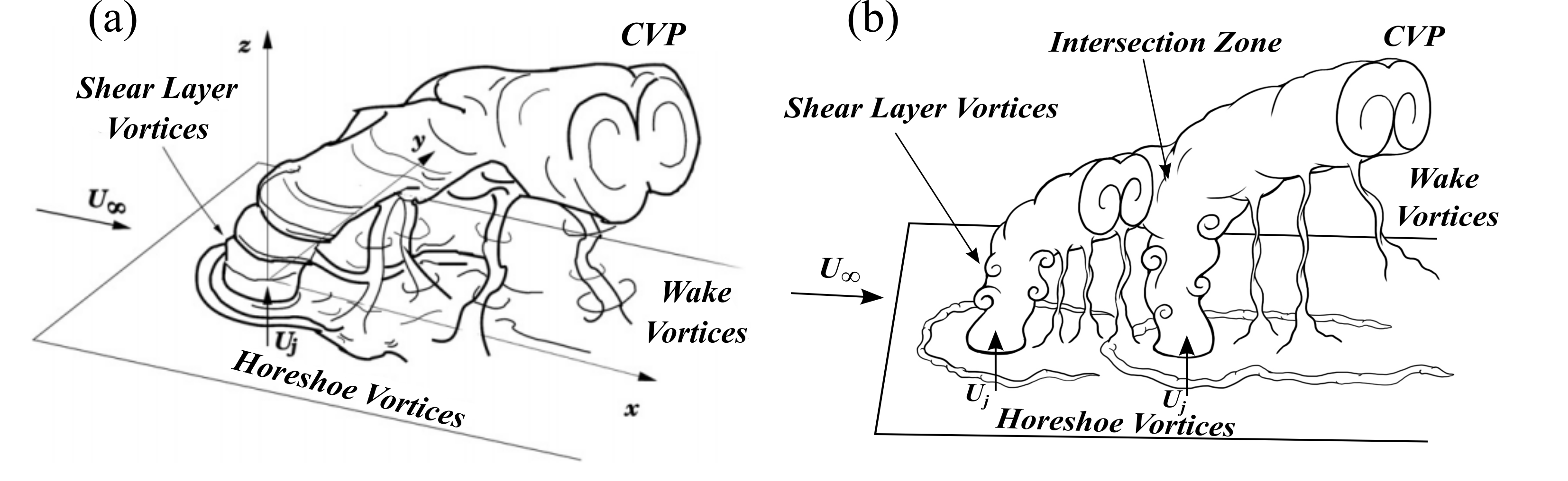
Figure 1: Schematic illustration of the single-nozzle JICF[1] and twin-nozzle JICF.

Two important factors to understand twin-nozzle JICF are the bending trajectory and the three-dimensional vortex structure. The single-nozzle JICF is well studied by experimental measurements and numerical simulations. Different scaling factors have been used to derive the trajectory equation such as early works by Keffer and Baines[2]. Broadwell treated the jet as a point momentum source and chose $rd$ as the length scaling factor[3]:

$$\frac{y}{rd}=A{(\frac{x}{rd})}^{B}$$ (1)

where $r$ is the momentum-flux ratio and $d$ is the nozzle diameter. Smith and Mungal also found that compared with $d$ and $r^{2}d$, $rd$ fits better as the length scaling factor[4]. In Eqn. (1), $A$ is the mixing parameter usually between 1.2-2.6 and $B$ is the fitted constant which determines the trajectory bending for the front and rear jets ranging around 0.28-0.34. Muppidi performed numerical simulation on jet trajectories with velocity ratios of 1.5 and 5.7 and proposed an similar analytical expression using $rd$ as the length scale factor[5]. The trajectory of twin-nozzle JICF has received less attention. Experiment been studied by Schwendemann et al.[6, 7, 8], but the scaling equation has not been proposed.

When the jet moves downstream along the trajectory, vortices are generated due to the interaction between jet and main-flow, including shear layer vortices (SLV), counter-rotating vortex pair (CVP), horseshoe vortices and weak vortices. Because of the large velocity difference between the mainstream and the jet, shear layer vortices are caused by Kelvin-Helmholtz instability. SLV are the dominant structure in the near field of the jet which exist on the windward and leeward of the jet and move downstream along the jet trajectory[9, 10]. The near-field vortex ring rolls up, tilts, folds, and interacts in the process of moving downstream, and finally forms kidney shape counter-rotating vortex pair as the dominant structure in the far-field[4, 11, 12]. Horseshoe vortices[13, 14] are formed around the jet in the boundary layer due to the blocking effect of the jet on the mainstream. The formation and rolling of the horseshoe vortices may be a periodic phenomenon, and its frequency is similar to the periodic separation of the wake vortices. Wake vortices are formed due to the separation of the mainstream boundary layer. It is perpendicular to the wall and connects it with the deflecting jet, and its separation has a certain frequency, which is significantly affected by the velocity ratios[15]. These vortex structures and their generation, development, propagation and the final fragmentation are mainly determined by the density ratio, the velocity ratio, and the momentum flux ratio. Hot wire velocity measurement were used to conducted experimental research on the shear layer vortex frequency. Huang put the hot wire in the single jet shear layer to measure the power spectral density function under different velocity ratios[16]. Getsinger et al. also used the hot wire to measure the relationship between SLV frequency and density ratio of single-nozzle JICF[17]. Some of recent studies[12] have focused on the movement frequency of shear layer vortex and find improvement in JICF mixing when forcing is applied at the specific values of the Strouhal number. The structure and dynamics of the vortices of twin-nozzle JICF are complicated due to the various interaction between the front and rear jets in the twin-nozzle JICF.

There are several reports on the experimental study of the vortex structure change of the twin-nozzle JICF arranged in parallel. Savory et al. used the real-time digitization system to study the twin-nozzle JICF arranged in parallel and obtained the quantitative data from the visualized flow field[18]. Kolář et al. used hot wire anemometer velocimetry to study the vorticity distribution and turbulent vorticity transport characteristics of the twin-nozzle JICF in two arrangements of series and parallel[19]. Zang et al. used PIV and PLIF technology to study the formation and development of counter-rotating vortex pairs in parallel twin-nozzle at different jet spacing and velocity ratios[20].

However, there is few study about the tandem twin-nozzle JICF. Radhouane et al. used PIV measurement to study the mixing behavior of twin-nozzle and triple-nozzle oblique jets with various heights at different velocity ratios. It is found that the jet height and the velocity ratios affect the mixing process of the mainstream and the jet mainly through the flow field and vortex structure[21, 22]. Gutmark et al. also used PIV measurement to study the difference of single-nozzle JICF and twin-nozzle JICF under different velocity ratios. Features investigated include jet trajectory, mass entrainment, turbulent kinetic energy and the dynamical behavior. It is found that the velocity field behavior of the front jet of twin-nozzle JICF has the same tendency as single-nozzle JICF, when $r=3$ and $L=2d$[23]. One important parameter that is missing from this study is the jet spacing of the tandem twin-nozzle JICF, which determines the interference between the front and rear jet. The separation of the SLV and the shedding of the CVP are inherently unsteady, but the transient characteristic of vortex structure such as SLV under the jet-main flow and jet-jet interaction has not been reported. Therefore, high-frame rate measurement that can capture the unsteady characteristics of the flow field and further analyze the dynamics and interaction between the twin-nozzle JICF is indispensable, especially for high speed shear layer vortex interaction.

High repetition rate measurement can capture the transient unsteady dynamics of turbulent flow-field and provide detailed insights into the turbulence characteristics and complex interactions of the twin-jet in crossflow. Pulse burst lasers can generate several hundreds of high energy laser pulses at repetition rates up to 10 kHz$\sim$1 MHz[24], reaching mJ/pulse energy level in the UV region for a burst period as long as 100 ms[25]. Measurement using burst mode laser has achieved significant progress in recent decade. Pumping an optical parametric oscillator[26, 27] or a dye laser[28],the burst mode laser allows non-intrusive temporal-resolved three-dimensional (4D) combustion diagnostic of flame temperature[29], concentration of soot[30],and reactive intermediates[31]. The burst mode laser has been used in PLIF[32], PIV[33], Thomson scattering[34], Rayleigh scattering[35, 36], Raman scattering[37], and coherent anti-Stokes Raman scattering techniques[38]. Recent advance in the development of burst mode lasers includes three-legged coherent output for simultaneous measurement of high-speed multi-species and multi-parameters combustion imaging[39]. The high repetition rate pulse mode lasers have been used in optical measurement of various combustion systems including gas turbine model combustor, scramjet, and various turbulent flame flow fields and structures including swirling flames and reacting jet in crossflow[40]. Measurement using burst mode laser can be used to study the unsteady dynamics characteristics of turbulent flow-field. For example, Liu et al. used the high-speed rate simultaneous PIV/PLIF imaging to accurately measure the precessing vortex core production process of the swirling flame in the process of changing at different stable positions for the first time[41]. Yi et al. used high-speed PIV and OH-PLIF to study the reacting jet in crossflow, and analyzed the flame initiation and flame stabilization mechanism of auto ignition[42].

In this paper, we used the burst mode PIV measurement at 40 kHz to investigate the turbulent flow-field and jet-jet interaction twin-nozzle JICF compared with the single-nozzle JICF with different jet spacing and velocity ratios. The trajectory equation scaling are obtained through the velocity field. The velocity distribution downstream along the jet trajectory and the attenuation of the jet center-line velocity are analyzed. Effect of the front and rear jet interaction on the strength of the reverse flow region is obtained. Furthermore, the SLV on the windward and leeward sides of the front and rear jets are extracted and their intensity and dynamics are analyzed. Pressure distribution and the turbulence intensity of the flow field are also analyzed.

II Experimental setup for high-speed imaging

Figure 2 shows structural diagram of the twin-nozzle JICF setup, which is divided into the primary stage, the development stage and the secondary stage. The primary stage provides mainstream. The development stage is a contraction structure to accelerate the mainstream. The cross sectional size of the secondary stage is 40 mm wide $\times$ 115 mm high $\times$ 295 mm long, surrounded by quartz glass for optical diagnosis. The two nozzles with the same diameter ($d$=4 mm) are installed in the secondary stage with jet spacing ($L$). The tracer particles are carried by the air and enter from the nozzle. The experimental conditions under investigation are listed in table  1, including test cases with velocity ratios at 3, 5, 7 and the jet spacing at 2$d$, 3$d$, and 4$d$, while the jet velocity ($V_{j}$) is 10 m/s and the main-flow velocity varied from 1.43 m/s to 3.33 m/s. Since the tracer particles are carried by a large amount of air, the density of both the jet and main-flow in all cases are constant at 1.293 kg/m³.

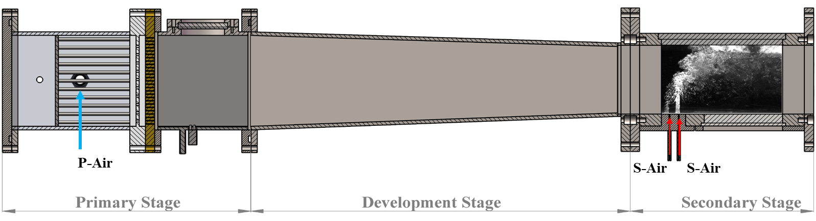
Figure 2: Schematic diagram of twin-nozzle JICF.

Table 1: Experimental conditions

case number	jet spacing $L$	main-flow velocity $U$ (m/s)	velocity ratio $r=V_{j}/U$
0	2$d$	3.33	3
1	2$d$	2.00	5
2	2$d$	1.43	7
3	3$d$	3.33	3
4	3$d$	2.00	5
5	3$d$	1.43	7
6	4$d$	3.33	3
7	4$d$	2.00	5
8	4$d$	1.43	7

The schematic diagram of the 40 kHz high-repetition-rate PIV system is presented in Fig. 3. The high repetition rate burst laser system consists of a flashlamp-pumped Nd:YAG burst mode laser (Spectral Energies, Quasimodo 1000), which has 100 kHz, 10 ms burst, 10 ns width, 100 J output. The PIV measurement was recorded using 532 nm laser, which was expanded to a 45 mm-height using three cylindrical lenses. The laser sheet thickness was around 0.2 mm and it enters to the secondary stage of the setup from the rear. The PIV signal is captured by the high-speed CMOS camera (Photron SA-Z) with a normal lens (Nikkon 50 mm f/1.4 G) and telephoto lens (Nikon AF-200/4d). The far field of the twin-nozzle JICF can be recorded using the short focal lens, and the trajectory of the twin-nozzle JICF and the intersection of the front and rear jet can be analyzed globally. The near-field region of twin-nozzle JICF can be recorded by the telephoto lens, and the reverse flow region and the shear layer vortex can be carefully analyzed. For the experimental conditions with jet velocity of 10 m/s and the characteristic length scale of 4 mm, Al₂O₃ tracer particles with the diameter of 1 $\mu$m are selected and the Stoke number ($Sk$) is calculated to be about 0.1, which satisfies the tracer conditions. The PIV images are calculated using the commercial software (Davis 8.4, LaVision) with multipass cross-correlation with decreasing size windows: from 32$\times$32 pixel square weighted with 75% overlap (1 pass) to 24$\times$24 pixel adaptive weighted with 50% overlap (2 pass). Figure 3(b) shows the time sequence of PIV experiment.

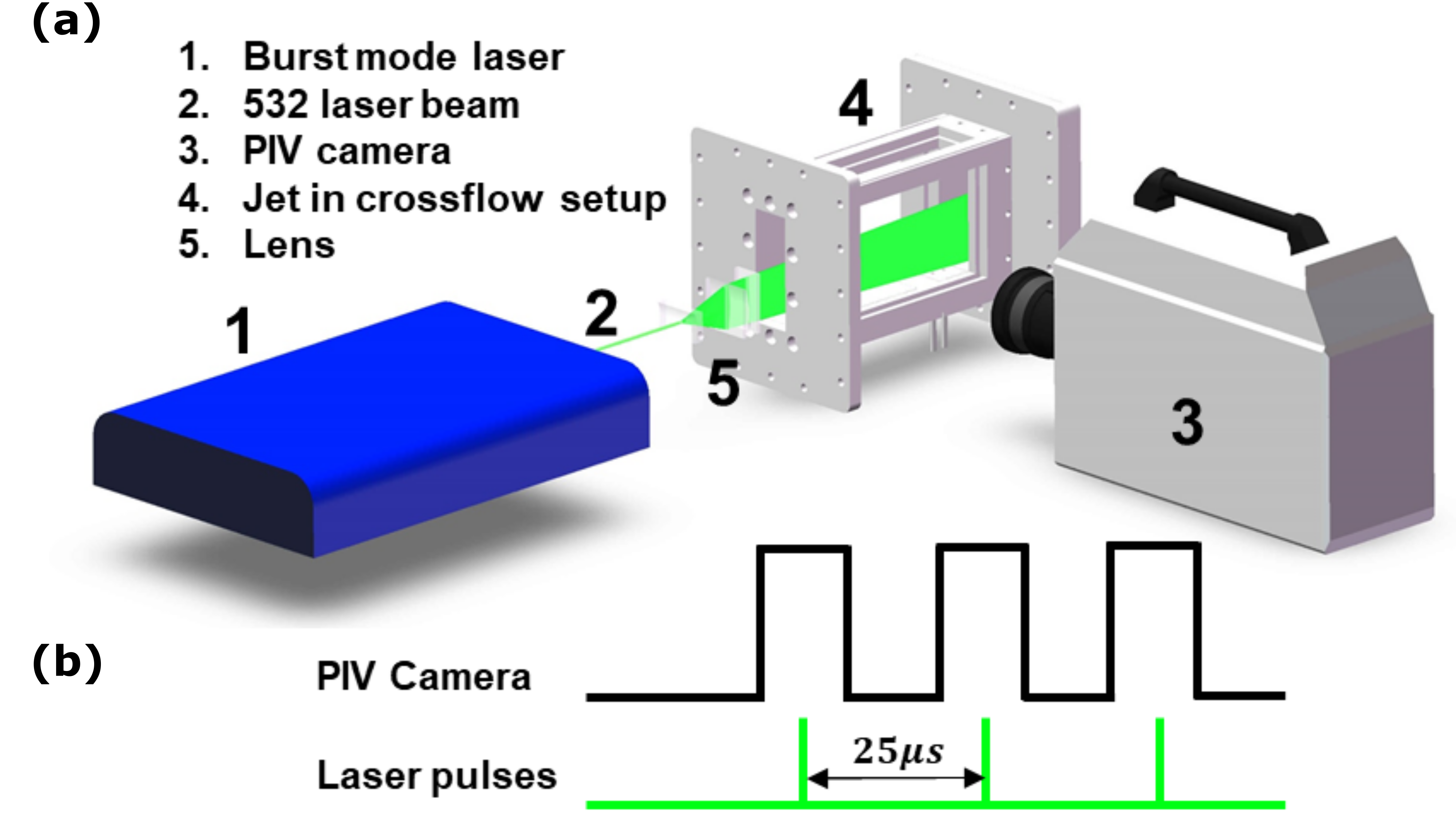
Figure 3: (a) Schematic drawing of the high-speed diagnostic system (b) Time sequence.

III Results and discussions

III.1 Trajectory

As shown in Fig. 4(a), the large visual field can be used to analyze the global flow field of the twin-nozzle JICF. The position of the intersection of the front and rear jets and the jet trajectory curve can be fitted more accurately. Comparing with the single-nozzle JICF shown in Fig. 4(b), the front and rear jets are ejected from the nozzles with the spacing of $L$. Under the effect of the mainstream, they interact and produce various of unsteady flow field structures, and finally merge into a mixed jet to move downstream. In order to analyze the more detailed vortex dynamic characteristics, a telephoto lens is used to photograph the near-field area of the jet surrounded by the red rectangle in Fig. 4(a), and the time series images as shown in Fig. 4(c) are obtained.

The qualitative changes in the flow field can be clearly observed from the visualization results. The yellow arrows in the figure refer to the large-scale shear layer vortex, and the red and blue arrows surround the shear layer vortices. They are produced by the interaction between the jet and the mainstream. Because of the Kelvin-Helmholtz instability, they are distributed on both sides of the jet[17, 43]. The red arrows indicate the direction of rotation of the shear layer vortex on the windward side is counterclockwise, and the blue arrows indicate that the direction of rotation of the shear layer vortex on the leeward side is clockwise. These two kinds of vortices appear periodically and alternately move downstream along the jet trajectory, and eventually merge, mix and break up during the transportation process. The green arrows in the figure point to the wake vortices. They are distributed between the jet and the wall, and their position depends on the pressure distribution in the flow field[1].

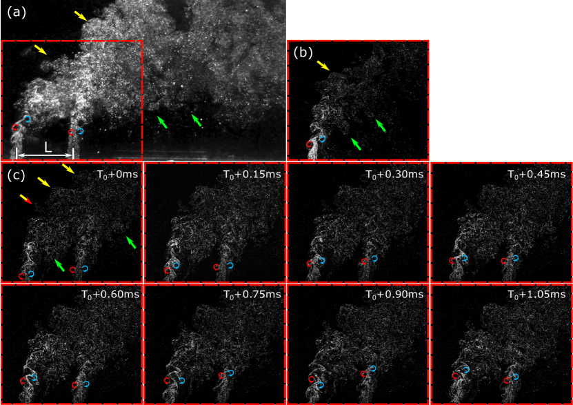
Figure 4: $r$=7, $L$=4$d$, the instantaneous PIV images of (a) Large visual field of twin-nozzle JICF (b) Near field of single-nozzle JICF (c) Near field of twin-nozzle JICF.

In order to quantitatively analyze the interaction of the front and rear jets and the unsteady motion of the SLV, the trajectory are analyzed firstly. Figure 5 (a) shows the mean flow field of the twin-nozzle JICF with different spacing and velocity ratios. The black lines are the trajectory curves of the front jet and the back jet taken at the point of maximum velocity. Due to the blocking effect of the front jet on the main-flow, the penetration depth of the rear jet is much greater than that of the front jet, so the front and rear jets meet during the downstream transportation. The black triangle is the intersection of the front and rear jets. The degree of deflection of the front jet is defined as $\alpha$. The area between the jet exit and the intersection is the separation region of front and rear jets, and the area above the intersection is the mixed region. When the velocity ratio is fixed, as the jet spacing increases, the area enclosed by the front and rear jets and the wall increases. As shown in Fig. 6 (a), we compared the trajectory of the single-nozzle JICF with the front and rear jet of twin-nozzle JICF at $r$=3, and it can be found that due to the interaction between the front and rear jets, the depth of the rear jet is much higher than that of the front jet than the single jet. From the twin-nozzle JICF trajectory, we can also fit to get the effective velocity ratio $r^{\prime}$ using Eqn. (1) to quantify the degree of interaction of front and rear jets, as shown in Table 2.

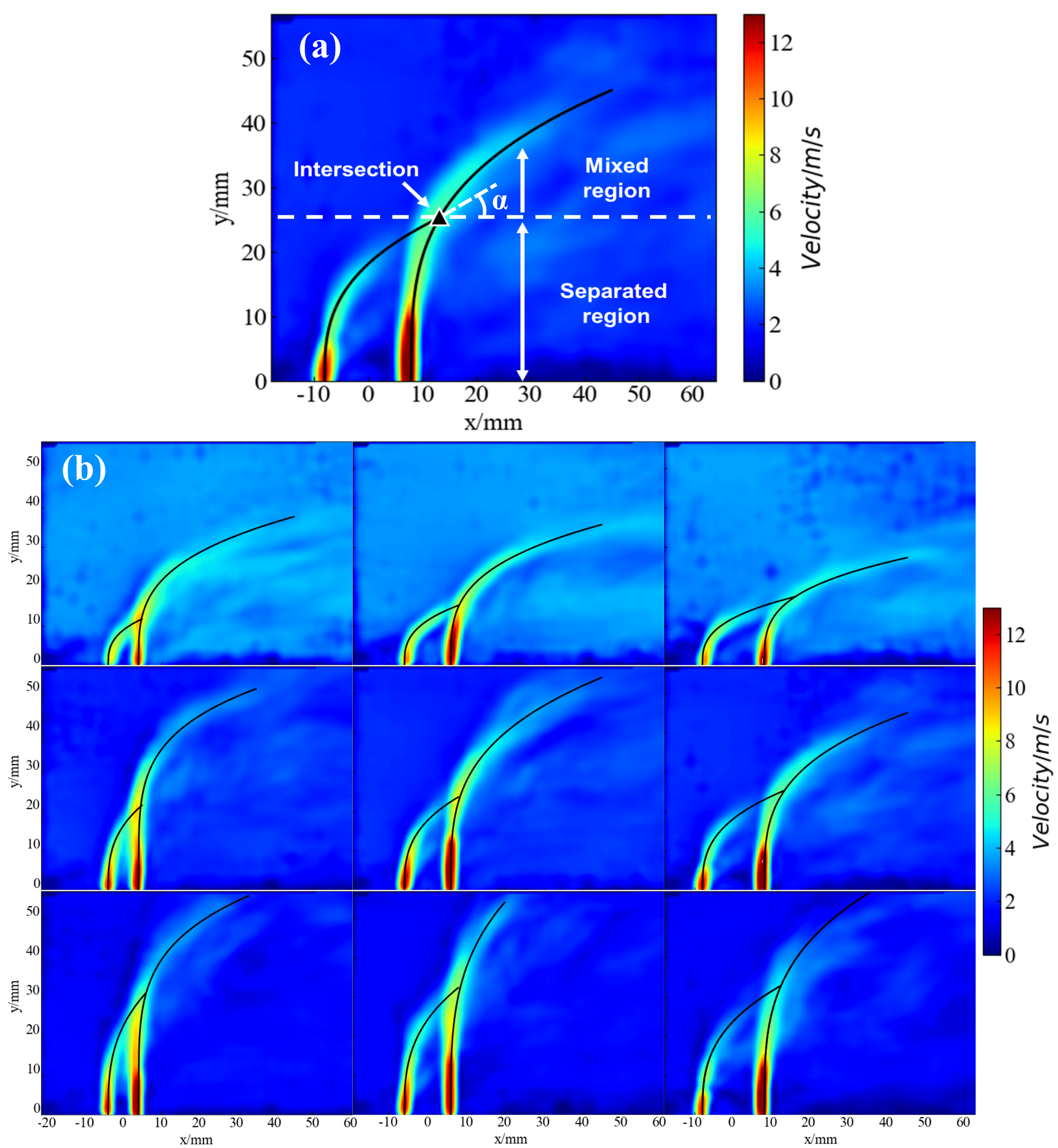
Figure 5: Contours of time-averaged velocity field.

Table 2: velocity ratio ($r$) of the twin-nozzle JICF and the effective velocity ratio ($r^{\prime}$) obtained by fitting with single-nozzle JICF equation with the $r^{\prime}/r$ ratio in the bracket

$r$	$r^{\prime}_{2d}$		$r^{\prime}_{3d}$		$r^{\prime}_{4d}$
	front jet	rear jet	front jet	rear jet	front jet	rear jet
3	4.08 (1.36)	9.26 (3.09)	3.69 (1.23)	7.80 (2.60)	3.58 (1.19)	5.91 (1.97)
5	7.83 (1.57)	14.03 (2.81)	6.29 (1.26)	12.54 (2.51)	4.96 (0.992)	10.08 (2.02)
7	12.05 (1.72)	18.46 (2.64)	8.95 (1.28)	17.15 (2.45)	6.53 (0.933)	14.34 (2.05)

As the twin-jet trajectories are elevated, the ratios of $r^{\prime}/r$ are greater than 1, which indicate the degree of jet-jet interaction and deviation of the behavior of twin-nozzle JICF compared to that of the single-nozzle JICF. Several trends can be clearly observed. First, the $r^{\prime}/r$ ratio decreases as the jet-jet distance increases, indicating the decrease of jet-jet interaction. Second, the $r^{\prime}/r$ ratio of the rear jet is higher than the front jet, showing that the rear jet lifting is higher than the front jet. But the lifting of the rear is observed to be less pronounced as the velocity ratio increased. The front jet, on the contrary, demonstrating an increasing $r^{\prime}/r$ ratio as the jet velocity ratio increases, although the absolute values of $r^{\prime}/r$ ratio is smaller. It is noted that when the jet spacing is $4d$, the $r^{\prime}/r$ ratio of the front jet decreases to slightly below 1 for the $r=5$ and $r=7$ cases. This is purely due to the fitting procedure that produced slightly lower value than expected These two values (0.992 and 0.933) can be viewed as 1, indicating that the front jet behaves as single-nozzle jet when the jet spacing is $4d$.

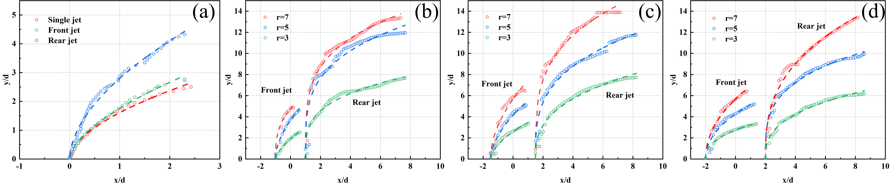
Figure 6: The points of maximum velocity and trajectory fitting (a) single-nozzle JICF and twin-nozzle JICF; (b) $L$=2$d$; (c) $L$=3$d$; (d) $L$=4$d$.

We now give a scaling equation for twin-nozzle JICF trajectory. As shown in Fig. 6, the line of the maximum average velocity in the time-average velocity field is defined as the jet trajectory curve. We first use an alternate form of the scaling equation as the starting point with the jet diameter $d$ as the scaling factor and the the velocity ratio ($r$) only on the r.h.s. of the equation.

$$\frac{y}{d}=A(r)^{C}{(\frac{x^{\prime}}{d})}^{B}$$ (2)

where $L$ is the jet spacing, $x^{\prime}=x\pm\frac{L}{2}$ is the corrected horizontal distance. We introduce a new parameter $C$ here. For single-nozzle JICF scaling form in Eqn  (1) , we have the simple relation $C=1-B$; but for twin-nozzle JICF, $C$ and $A$ are also related to the reduced jet spacing $l=L/d$ that determines the jet-jet interaction. Using Eqn. (1) as the scaling function:

$$\begin{cases}\frac{y_{\text{front}}}{d}&=(0.5+0.1l)r^{(-0.2l+1.5)}{(\frac{x^{\prime}}{d})}^{0.5}\\ \frac{y_{\text{rear}}}{d}&=(3.2-0.5l)r^{(0.1l+0.5)}{(\frac{x^{\prime}}{d})}^{0.3}\end{cases}$$ (3)

This can be re-arranged to:

$$\begin{cases}\frac{y_{\text{front}}}{r^{(1.5l-5)}d}&=(0.1l+0.5){(\frac{x^{\prime}}{r^{(1.5l-5)}d})}^{0.5}\\ \frac{y_{\text{rear}}}{r^{(1.5l-5)}d}&=(-0.5l+3.2){(\frac{x^{\prime}}{r^{(1.5l-5)}d})}^{0.3}\end{cases}$$ (4)

with the length scaling term is $r^{(1.5l-5)}d$. The reduced jet spacing $l=L/d$ appears in both the mixing term and the length scaling term.

It is noted that the scaling equation should be used for $l$ values that are smaller than 4. When $L$ is $4d$, the scaling length term is reduced to the single-nozzle JICF scaling term $rd$. This finding explains the thumb rule that when the jet distance $L$ is greater than 4 time nozzle diameter, the jet trajectory can be deemed single-nozzle JICF without the jet-jet interaction. The scaling equations were also compared the trajectory obtained by Gutmark[23], as shown in Fig. 7, in good agreement.

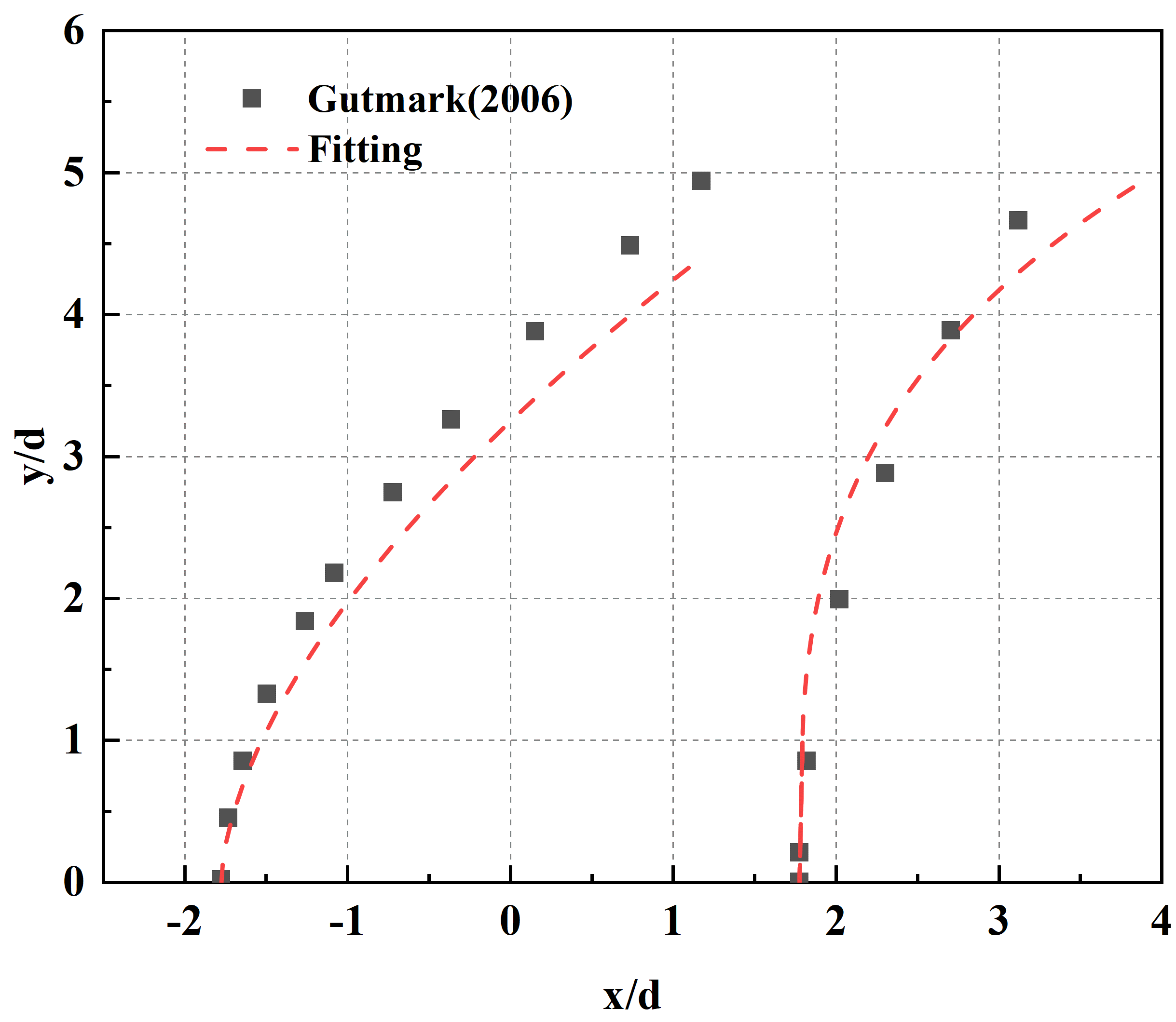
Figure 7: Validation of the scaling law of twin jet trajectories with previously published data.

III.2 Time averaged velocity distribution

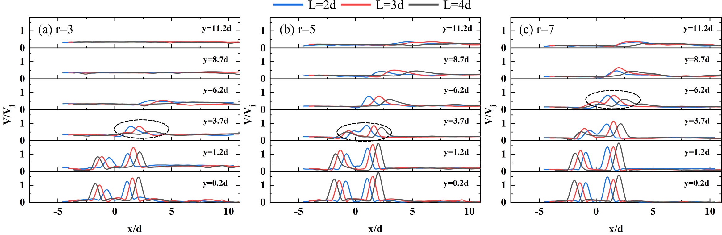
Figure 8: Stream-wise development of the mean velocity profiles from $y$=0.2$d$ to 11.2$d$ along symmetry plane for twin-nozzle jet at (a)$r$=3; (b)$r$=5; (c)$r$=7.

The profiles of mean velocity extracted at downstream location from $y$=0.2$d$ to 11.2$d$ are presented in Fig. 8 to provide a quantitative comparison between twin-nozzle JICF of different velocity ratios and jet spacing. The large visual field can be used to analyze the mean velocity changes in different areas including the front and rear jet separation region and mixed region. A cross-sectional view of the area’s mean velocity $V(V={\sqrt{U^{2}+V_{j}^{2}}})$, and the jet velocity $V_{j}$ is used for normalization. Many researches have applied similar velocity profile forms to study the development and evolution of single-nozzle JICF. For example, Bidan[44] through studied the variation of mainstream velocity on different cross-sections to study the development of JICF. Wen et al.[45] studied the horizontal and vertical average velocities of various positions downstream of the inclined jet. And Dai[46] also used this velocity profile method to compare experimental data with simulated data.

The origin of the coordinate system is placed at the midpoint of the center-line of the front and rear nozzles. It can be seen from the figures that the peak velocity of the rear jet is significantly larger than that of the front jet, indicating that the impact of the mainstream on the front jet makes its velocity slightly smaller than that of the rear jet, and the penetration depth of the rear jet is greater. The velocity ratio and jet spacing have a greater influence on the jet deflection position. When the velocity ratio $r$=3, at $y$=3.7$d$, the front and rear jets with the distance of 4$d$ and 3$d$ have a fusion trend. The front and rear jets with a spacing of 2$d$ merge obviously, and the velocity is in a single peak state. At $y$=6.2$d$, the jet is completely deflected, and the velocity is close to the mainstream velocity. When the velocity ratio $r$=5, at $y$=3.7$d$, the front and rear jets with a spacing of 3$d$ and 4$d$ are clearly separated. The front and rear jets with a spacing of 2$d$ have shown a significant fusion trend. At $y$=6.2$d$, the front and rear jets with different spacing are completely fused, and the velocity presents a single peak state. Then the jet deflects obviously at $y$=11.2$d$, and the velocity is close to the mainstream velocity. When the velocity ratio $r$=7, at $y$=6.2$d$, the front and rear jets with a spacing of 2$d$ have been completely fused, and the front and rear jets with a spacing of 3$d$ and 4$d$ have a clear fusion trend. At $y$=8.7$d$, the front and rear jets are completely fused, indicating that the greater the velocity ratio, the greater the jet spacing, and the farther the front and rear jets are fused. These two factors both inhibit the fusion of the front and rear jets.

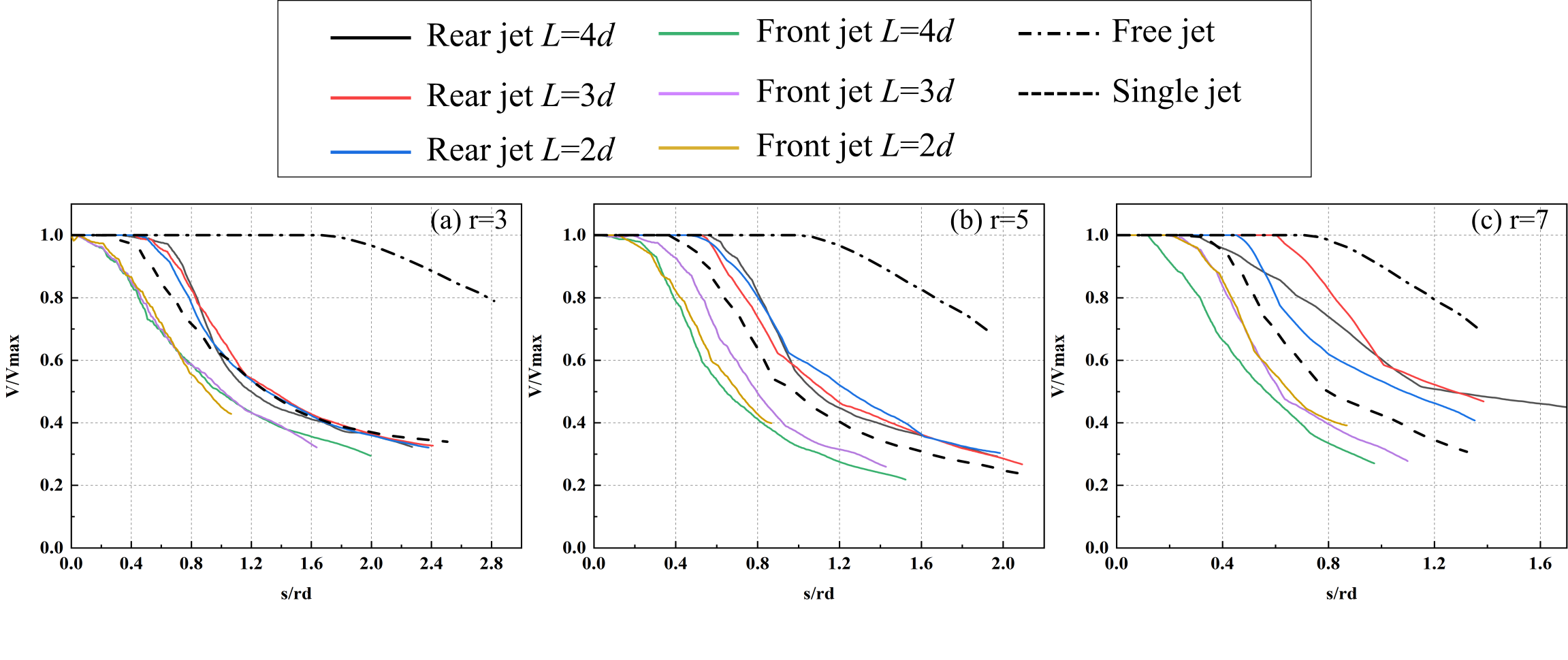
Figure 9: Effect of the velocity ratios and jet spacing on center-line velocity decay and comparison with single-nozzle JICF and free jet[47].

Under the effect of the main-flow, the cross-sectional area increases, and the initial momentum of the jet is redistributed to a plane that deviates from the center-line of the jet. And the CVP begins to develop and brings more jet flow downstream, causing the velocity along the trajectory decline. Using the jet trajectory equation (4), the trajectory length can be obtained. Figure 9 shows the velocity decline profiles of the front and rear jets along the trajectory of the twin-nozzle JICF, and compares it with the single-nozzle JICF. The jet velocity is normalized by the maximum jet velocity. It can be found that with different velocity ratios, the interaction between the front and rear jets and their interaction with the main-flow make it lose the characteristics of single jet. The center-line line velocity of the jet remains stable in the potential core area[23], and it begins to show a decay trend in the deflection area. It can be found that the shielding effect of the front jet makes the attenuation of the center-line velocity of the rear jet lower than that of single-nozzle JICF. And when the velocity ratio is 3, the decay trend of the center-line of the front jet of twin-nozzle JICF at different jet spacing is close to that of the rear jet, indicating that the jet spacing has little effect on the velocity decline trend at this time. As the velocity ratio increases to 5 and 7, the decay trend of center-line velocity of twin-nozzle JICF front jet is significantly less than that of single-nozzle JICF, and the degree of velocity decrease varies between different jet spacing. The conclusions we obtained through a large number of experimental measurements are different from the findings reported by Gutmark[23] that the velocity of the front jet is similar to that of the single jet. The reason may be that the trajectory changes caused by the interaction between the front and rear jets make the pressure between them change, which makes the velocity along the trajectory of the front jet decay faster.

When the jet start to develop downstream from the exit of the circular nozzle, its circular cross section gradually becomes elliptical, which is also one of the factors that cause the attenuation of the jet center-line velocity. Therefore, in this paper, the change of the center-line velocity of the free jet with the elliptical cross-section is compared with that of single-nozzle JICF. Since the free jet is not affected by the main-flow, its jet direction is the trajectory direction. Obviously, its potential core length is much larger than single-nozzle and twin-nozzle JICF. When $s$ is within the range of 5$d$, its center-line velocity remains mainly unchanged and then decreases. The decay trend is much smaller than that of single-nozzle and twin-nozzle JICF, which means that the existence of the mainstream has a greater impact on the decrease of the jet center-line velocity.

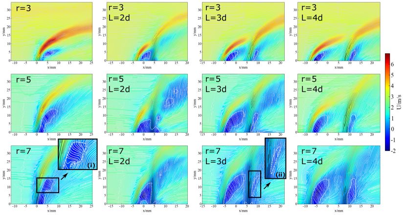
Figure 10: Horizontal velocity component U and zero streamline velocity contours

III.3 Reverse flow region analysis

When the mainstream moves around the jet like flow around a circular cylinder motion and is pulled back to the leeward side by the jet at the same time, the reverse flow region is formed. The reason is that when the jet flows downstream, an inverse pressure gradient is formed on the leeward side, making the flow direction opposite to the main-flow direction. Figure 10 (i) shows that the direction of the streamline is opposite to the mainstream direction in reverse flow region. The degree of blockage of the jet to the main-flow determines the strength of the reverse and the size of the reverse pressure gradient on the leeward side of the jet. Essentially, the reverse flow region should be a three-dimensional area. In this paper, only the two-dimensional velocity field distribution is obtained, so it is represented by a two-dimensional area. In order to clearly identify the reverse flow region, the near-field area of the jet is selected for analysis.

Figure 10 shows the horizontal velocity component and the streamline. The area enclosed by the white dashed line represents the reverse flow region. The main-flow comes into contact with the front jet and moves around it, forming a reverse flow region between the front and rear jets. This part is called the front reverse flow region, which continues to move downstream, bypassing the rear jet, and forms the rear reverse flow region on the leeward side of the rear jet. The reverse flow region provides upward lift for the curved jet and promotes its movement away from the wall. Therefore, it determines the penetration of the jet, and a stronger reverse flow will also enhance the penetration of the jet. In order to quantitatively analyze the effect of jet spacing and velocity ratio on the strength of the reverse flow of the single-nozzle JICF and front and rear reverse flow of twin-nozzle JICF. We define the parameter RZ as the strength of the reverse flow region, and its expression is:

$$RZ=\iint_{S}Ud\sigma$$ (5)

in which $S$ is the area of the reverse flow region, and $U$ is the horizontal velocity component. Figure 11 shows strength of the reverse flow region of different velocity ratios and different jet spacing. The green part represents the reverse flow region of single-nozzle JICF. The red part represents the front reverse flow region of twin-nozzle JICF, and the blue part represents the rear reverse flow region. It can be found that when the jet spacing is fixed, as the velocity ratio increases, the RZ of the front and rear jet gradually increases, and the reason is that the jet has a stronger blocking effect on the mainstream and produce a larger reverse pressure gradient, and the reverse force on the mainstream is stronger. And when the velocity ratio increases, the pressure gradient on the leeward side of the front and rear jets extends farther from the wall in the jet direction, and the longer the action length, so the shape of the reverse flow region also elongates in the jet direction. Under the same experimental conditions, the RZ of the front jet is always greater than that of the rear jet. The reason is that the rear jet provides an additional blocking effect on the part of the main-flow limited between the front and rear jets, thereby forming a greater back pressure gradient and RZ. Similarly, the RZ of single-nozzle JICF is always smaller than that of the front jet of twin-nozzle JICF, and it is always greater than the rear jet, which can also be explained by this reason.

In the case of constant velocity ratio, as the jet spacing increases, RZ increases too. The reason is that the jet spacing increases, the fluid restricted between the front and rear jets increases, and the distance of the reverse force exerted by the front jets on it is longer, making the reverse flow region stronger. When the main-flow continues to move through the restricted area, its velocity increases due to the effect of the main-flow. As the jet spacing increases, the greater the velocity of the fluid bypassing the rear jet, the higher the strength of the reverse flow region of it.

It is also found that when the reduced jet spacing ($l$) is 2, the shape of the reverse flow region changes irregularly, and the front reverse flow region merges with the rear reverse flow region. As the jet spacing decreases, the front and rear jets simultaneously pull and mix with part of the main-flow confined between them, causing irregular changes in the flow field. And with the increase of the velocity ratio, the lift effect of the fluid near the jet is greater, which makes the shape of the reverse flow region elongate in the direction of the jet, and its lifting behavior is obvious, as shown in Figure 10 (ii), the streamline direction is upward, and the reverse flow region moves in the direction of the jet.

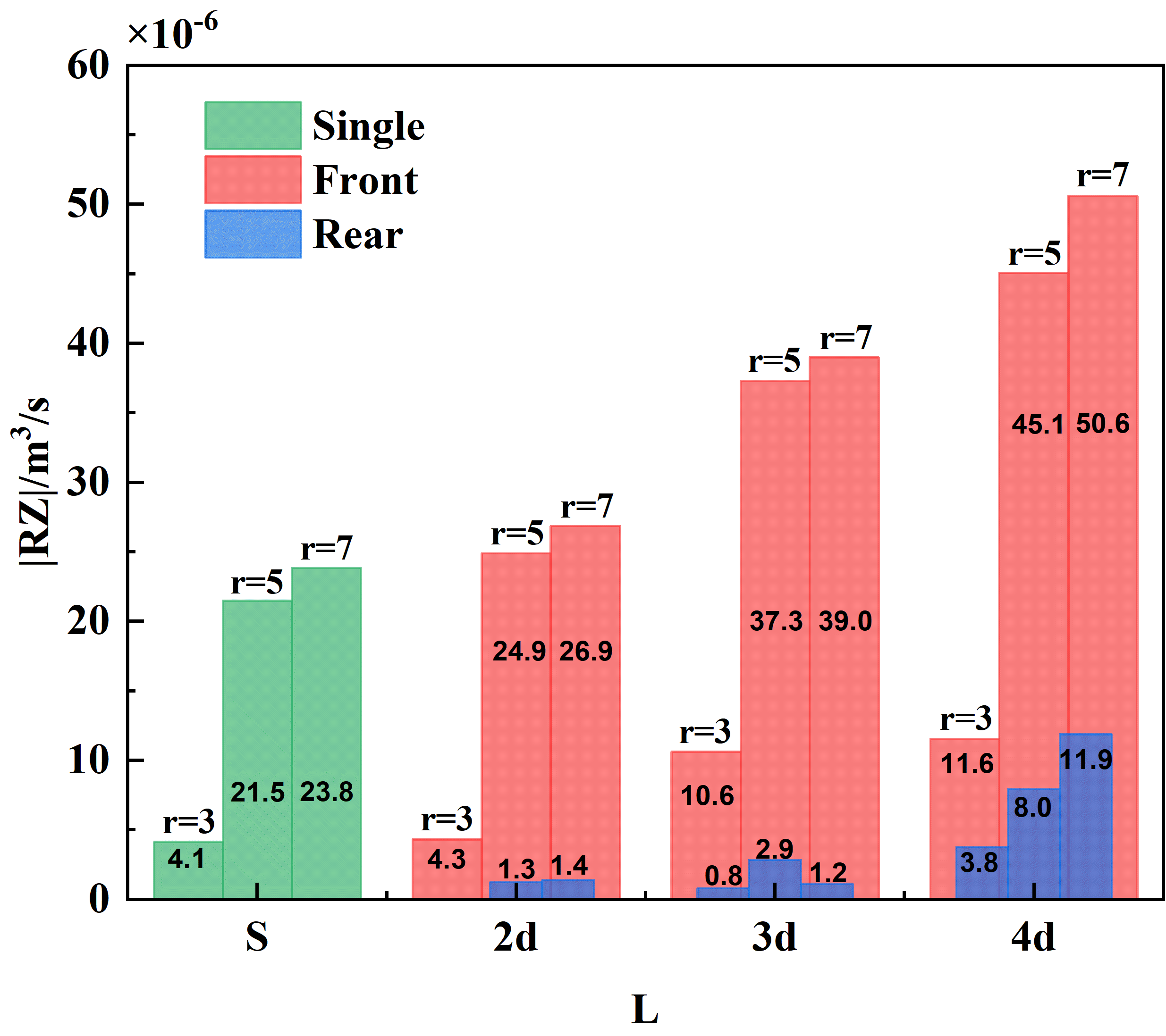
Figure 11: The strength of the reverse flow region of different velocity ratios and different jet spacing.

III.4 Vortex Dynamics

The formation, development, propagation and final breaking of the shear layer vortex (SLV) and counter-rotating vortex pair (CVP) in JICF are main factors for the development of the cross-sectional shape and size along the trajectory and the enhancement of mixing. The SLV is formed due to the Kelvin-Helmholtz instability from velocity difference of jet and main-flow, usually in pairs of opposite direction, as shown in Fig. 12(a). Due to the existence of strong stretching of shear layer, we calculated the vorticity from PIV measurement using Liutex method[48].

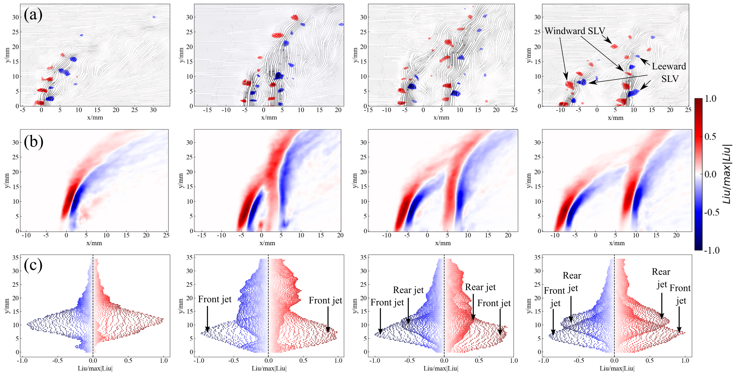
Figure 12: (a) Instantaneous vorticity field; (b) Time-averaged vorticity field; (c) The quantitative evolution of shear layer vortex strength of $r$=5.

Liutex is a vector with direction and magnitude, whose direction is the local axis of rotation, and the magnitude is the fluid rotation strength that we use as the shear layer vortex strength indicator. Fig 12(a) shows the Liutex vorticity of single-nozzle and twin-nozzle JICF when $r$=5 calculated from the experimental data. The direction of the SLV (red) on the windward side is counterclockwise and the magnitude is positive. The direction of leeward side SLV (blue) is clockwise and its magnitude is negative. The windward and leeward SLV are distributed on both sides of the jet center trajectory and the rows of opposite-signed vortices are arranged in an alternate fashion, forming a single row vortex and a double row vortex street. Due to the intersection of the front and rear jets in the process of transporting downstream, the double row vortex merges to form a single row. During the continued movement, it continuously splits and then breaks into small-scale vortices, as suggested by Zang et al. that it originates from the annihilation of the CVP[20].

Figure 12(b) shows the contours of the mean field of Liutex. It is found that the front jet produces greater deflection than the rear jet at different jet spacing, which is similar to the results observed by Gutmark[23] before. Moreover, the Liutex intensity of the SLV on the windward and leeward sides of the front jet is slightly larger than that of the rear jet, which confirms the viewpoints that the front jet shields the rear jet. Figure 12(c) counts the Liutex at each height within 35 mm downstream of the jet exit when the velocity ratio $r$=5, and normalizes it with the maximum value, giving the quantitative evolution law of the shear layer vortex along the jet direction. The red and blue parts in the figure respectively represent the intensity distribution of the shear layer vorticity on the windward side and the leeward side at different heights, which are approximately symmetrically distributed along the axis $x$=0. And Liutex showed a trend of first increasing and then decreasing during the movement from the jet exit to the downstream. The single-nozzle JICF shows a single-peak trend and the twin-nozzle JICF shows a double-peak trend, indicating that the jet is dominant at the jet exit, and vortex generated by rotation is small. At the position where the jet is about to deflect, the vortex generated by the rotation reaches the maximum value and a peak phenomenon occurs. Furthermore, in the process of downstream transportation, the windward and leeward shear layer vortices alternately move, merge and mix with each other, and their strength presents a dynamic downward trend. Finally, due to the complete deflection of the jet, the vortex generated by the rotation is reduced, and the Liutex vorticity is also reduced.

It was also found that the Liutex peak of single-nozzle JICF appeared at the position of $y$=10 mm downstream of the exit. The peak of the front jet of the twin-nozzle JICF at different spacing appeared in the range of 5-10 mm. However, the peak position of rear jet of twin-nozzle JICF with a spacing of 2$d$ is not obvious, and when the spacing is 3$d$ and 4$d$, the peak of the rear jet appears in the range of 10-15 mm downstream of the exit. And as the jet spacing increases, the Liutex peak of the rear jet gradually increases, indicating that the existence of the rear jet will reduce the peak value of the front jet, and the jet spacing has a significant impact on the Liutex vortex of the rear jet. As the jet spacing increases, this effect gradually decreases.

Figure 13: Frequency (a)(b)(c), phase $\phi_{n}$ (d)(e)(f) and unwrapped phase $\phi_{nw}$ (g)(h)(i) of twin-nozzle JICF with different jet spacing

Figure 14: The Power spectral density of different jet spacing.

Figure 13 (a)(b)(c) show the frequency distribution contour diagrams under different jet spacing. It can be found that the shear layer vortex motion frequency on the windward and leeward sides of the jet is basically fixed between 1000 and 1600 Hz in the near-field region of the jet outlet, as the power spectral density shown in the Fig.14. In the process of developing downstream, the shear layer vortex is gradually broken, so there is no obvious characteristics frequency. The phase $\phi_{n}$ obtained by the Fast Fourier Transform (FFT) is shown in Fig. 13 (d)(e)(f), and by unwrapping it, the unwrapped phase $\phi_{nw}$ of Fig. 13 (g)(h)(i) can be obtained. The distribution of these quantities is shown in Fig.13 (g)(h)(i). It can be found that when $L$=2$d$ and 3$d$, the front jet shear vortex increases from 1 period by 7 periods, and the rear jet shear vortex increases from 1 period by 10 periods. However, when $L$=4$d$, the shear layer vortices of the front and rear jets bot increase from 1 period by 7 periods. The reason is that with the increase of the jet spacing, the mutual influence of the front and rear jets decreases, and the shear layer vortices in the interesting area have a large degree of fragmentation and a decrease in strength, which can also be found in Fig. 12.

III.5 The pressure distribution

The pressure distribution in the flow field is an important dynamic characteristic of fluid motion, which determines the force of the objects in the flow field, and is also the source of noise and vibration[50]. It can be solved based on the time-resolved PIV velocity field combined with the finite volume method, the direct integration method or the Poisson equation method. Gurka[51] proposed and verified the basic principle of reconstructing the pressure field based on the velocity field. Tanahashi[52] used PIV to reconstruct the pressure field to study the force of the flow around the cylinder. In this paper, we used the finite element method in FEniCSx package[53] and use arbitrary unit of the pressure and mainly investigate the pressure distribution here, since the air velocity is in the incompressible regime and the velocity field satisfies the divergence-free condition. Figure 15 shows the instantaneous pressure distribution distribution of single-nozzle and twin-nozzle JICF. The black solid and dotted lines represent the SLV on the windward and leeward side calculated in Section III.4. It can be found that the calculated pressure distribution almost overlap witht the vorticity distribution and the pressure at the center of the vorticity is the smallest, which is consistent with Hunt’s finding[54].

Figure 15: The instantaneous pressure and vorticity distribution of single-nozzle and twin-nozzle JICF.

Figure 16 shows the time-averaged pressure field in arbitrary unit. It can be found that the pressure on both sides of the nozzle outlet is relatively high, and the central pressure is relatively low. When $L$=2$d$, the local pressure at the intersection of the front and rear jets is the largest, as shown by the black boxes in the figure. The reason is that the rear jet has the strongest impact on the front jet, which increases the local pressure. Figure  17 shows the quantitative comparison between the average pressure in the intersection area and the deflection degree of the front jet. The local average pressure is calculated from the average pressure in the black boxes, and the deflection degree is defined in Fig. 5. It can be found that as the jet spacing increases from 2$d$ to 4$d$, the local average pressure decreases from 4.96 to 2.94, and the deflection degree of the front jet decreases from $42^{\circ}$ to $18^{\circ}$. Combining with the time-averaged vorticity field given in Fig. 12, it can be found that the pressure at the place with the largest vorticity is relatively small, which corresponds to the instantaneous results.

Figure 16: The time-averaged pressure distribution of single-nozzle and twin-nozzle JICF.

Figure 17: The deflection degree $\alpha$ of the front jet and the local average pressure of the intersection area.

III.6 Turbulent kinetic energy analysis

The degree of interaction between the front and rear jets of twin-nozzle JICF can be reflected by the instability of the flow-field. Twin-nozzle JICF in this experiment is a highly nonlinear turbulent flow, and the flow field is randomly pulsating in time series, which is in a highly disordered and chaotic state in space. The analysis of the turbulent kinetic energy[23] (TKE) of the flow field can understand the turbulence characteristics of the twin-nozzle JICF. The turbulent kinetic energy is the sum of the turbulent kinetic energy of many vortices of different sizes, which can be calculated by $TKE=\frac{1}{2}({u^{\prime}}^{2}+{v^{\prime}}^{2})$. Figure 18 shows the turbulent kinetic energy of the single-nozzle and twin-nozzle JICF with different velocity ratios and jet spacing. It can be found that the turbulent kinetic energy of the shear layer on the windward side is greater than that on the leeward side, regardless of whether it is a single-nozzle JICF or twin-nozzle JICF. The reason is that the windward side directly interacts with the main-flow, which increases the intensity of turbulence. And with the decrease of jet spacing, the turbulence intensity in the downstream mixing jet zone increases, indicating that the mutual interference of the front and rear jets will increase the turbulence intensity.

Figure 18: The plot of the turbulent kinetic energy distribution of (a)single jet, $r$=5; (b) $L$=2$d$, $r$=3; (c) $L$=3$d$, $r$=7; (d) $L$=2$d$, $r$=5; (e) $L$=3$d$, $r$=5; (f) $L$=4$d$, $r$=5.

Figure 19: The center-line turbulent kinetic energy of the single-nozzle JICF and twin-nozzle JICF with different jet spacing at different velocity ratios

It can be observed that the turbulence intensity reaches the maximum value due to the jet-crossflow interaction. The interaction between the front and rear jets makes the peak position of TKE of twin-nozzle JICF different from that of single-nozzle JICF. Therefore, the trajectory equation obtained in Section III.1 is used to quantitatively analyze the change trend of the center-line turbulent kinetic energy of the single-nozzle and twin-nozzle JICF with different jet spacing and velocity ratios, as shown in Fig. 19.

From Fig. 19 (a)(b)(c), it can be found that the TKE peak of single-nozzle JICF is located at about $s$=0.7$rd$. And due to the shielding effect of the front on the rear jet, the position of the TKE peak is ranked as follows: the rear jet of twin-nozzle JICF is farther than that of single-nozzle JICF and farther than the front jet of twin-nozzle JICF. It can also be found from the Fig. 19 (d)(e)(f) that when the velocity ratio is different, the TKE peak position of the rear jet of twin-nozzle JICF is always closer than that of the front jet, and with the increase of the velocity ratio, the peak value of the turbulent kinetic energy of the rear jet decreasing gradually.

IV Conclusions

The high-frequency Particle Image Velocimetry (PIV) technique was employed to examine the effects of jet spacing and velocity ratio on the structure and dynamic characteristics of the twin-nozzle jet in crossflow (JICF). This study provides a quantitative analysis of the flow characteristics and jet-jet interaction of the twin-nozzle JICF. Compared to the single-nozzle case, both the front and rear jet trajectories were elevated. The rear jet trajectory was raised due to the blocking effect of the front jet, while the pressure field of the rear jet contributed to the elevation of the front jet trajectory. The jet-jet interaction also resulted in a more pronounced velocity decay along the front jet trajectory compared to the rear jet. Consequently, the Strouhal frequency of the front jet’s shear layer vortices (SLV) was higher than that of the rear jet. The study further analyzed the jet trajectory and fusion process of the front and rear jets, jet center-line velocity attenuation, reverse flow region variation, SLV intensity and dynamic characteristics, pressure distribution, and turbulence kinetic energy. To summarize, the study yields the following conclusions:

• Jet Fusion and Trajectories: The velocity ratios and jet spacing promote the fusion of the front and rear jets. Due to the blocking effect of the front jet on the main flow, the rear jet exhibits stronger penetration. Trajectory equation with the scaling length $r^{(1.5l-5)}d$ were derived. The mainstream flow exerts a significant influence on the reduction of jet center-line velocity. The average velocity attenuation of both single-nozzle and twin-nozzle jets along the trajectory is substantially greater than that of a free jet. The attenuation of the front jet’s center-line velocity is greater than that of a single jet, while the rear jet exhibits less attenuation compared to the single jet. As the velocity ratio increases, the decay trends of center-line velocity with varying jet spacing become more pronounced. During downstream transport, the jet mix with the main flow, redistributing the initial momentum of the jet and forming a reverse flow zone (RZ), which is strongly affected by the velocity ratio and jet spacing. When the velocity ratio is constant, the RZ of the single-nozzle JICF is smaller than that of the front jet in the twin-nozzle configuration, but larger than that of the rear jet. As both the velocity ratio and jet spacing increase, the RZs of the front and rear jets expand, with the front jet consistently having a larger RZ than the rear jet.

• Vortex Dynamics: Using Liutex vortex identification theory, frequency analysis of the shear layer vortices (SLV) on the windward and leeward sides of the front and rear jets reveals that SLVs gradually break down into smaller vortices during downstream transport due to mixing between the main flow and the jets. The local pressure at the vortex center is the lowest. As jet spacing decreases, the local pressure at the intersection of the front and rear jets increases, leading to a greater deflection angle of the front jet.

• Turbulence Kinetic Energy (TKE): Analysis of turbulence kinetic energy reveals that the TKE of the shear layer on the windward side of the jet is consistently greater than that on the leeward side. As jet spacing decreases, the turbulence intensity in the downstream mixed region increases. Along the jet center-line, TKE initially increases and then decreases, forming a single peak. Due to the shielding effect of the front jet in the twin-nozzle JICF configuration, the peak TKE location for the single-nozzle JICF is closer to the nozzle compared to the front jet of the twin-nozzle JICF.

Funding

National Natural Science Foundation of China (NSFC) (52076137, 91941301); Natural Science Foundation of Shanghai (21ZR1431300).

References

- Fric and Roshko [1994] T. F. Fric and A. Roshko, Journal of Fluid Mechanics 279, 1 (1994), publisher: Cambridge University Press.
- Keffer and Baines [1963] J. F. Keffer and W. D. Baines, Journal of Fluid Mechanics 15, 481 (1963).
- Broadwell and Breidenthal [1984] J. E. Broadwell and R. E. Breidenthal, Journal of Fluid Mechanics 148, 405 (1984), publisher: Cambridge University Press.
- Smith and Mungal [1998] S. H. Smith and M. G. Mungal, Journal of Fluid Mechanics 357, 83 (1998), publisher: Cambridge University Press.
- Muppidi and Mahesh [2005] S. Muppidi and K. Mahesh, Journal of Fluid Mechanics 530, 81 (2005).
- Schwendemann [1973] M. F. Schwendemann, Northrop Aircraft Division, Hawthorne, CA, Rept. NOR , 73 (1973).
- Ziegler and Wooler [1971] H. Ziegler and P. T. Wooler, Journal of Aircraft 8, 414 (1971).
- Isaac and Jakubowski [1985] K. M. Isaac and A. K. Jakubowski, AIAA Journal 23, 1679 (1985).
- Andreopoulos [1985] J. Andreopoulos, Journal of Fluid Mechanics 157, 163 (1985).
- Kelso et al. [1996] R. M. Kelso, T. T. Lim, and A. E. Perry, Journal of Fluid Mechanics 306, 111 (1996), publisher: Cambridge University Press.
- Cortelezzi and Karagozian [2001] L. Cortelezzi and A. R. Karagozian, Journal of Fluid Mechanics 446, 347 (2001), publisher: Cambridge University Press.
- Karagozian [2010] A. R. Karagozian, Progress in Energy and Combustion Science 36, 531 (2010).
- Baker [1979] C. J. Baker, Journal of Fluid Mechanics 95, 347 (1979), publisher: Cambridge University Press.
- Kelso and Smits [1995] R. M. Kelso and A. J. Smits, Physics of Fluids 7, 153 (1995).
- Krothapalli et al. [1990] A. Krothapalli, L. Lourenco, and J. M. Buchlin, AIAA Journal 28, 414 (1990).
- Huang and Lan [2005] R. F. Huang and J. Lan, Physics of Fluids 17, 034103 (2005), number: 3.
- Getsinger et al. [2014] D. R. Getsinger, L. Gevorkyan, O. I. Smith, and A. R. Karagozian, Journal of Fluid Mechanics 760, 342 (2014), publisher: Cambridge University Press.
- Savory and Toy [1991] E. Savory and N. Toy, Journal of Fluids Engineering 113, 68 (1991).
- Kolar et al. [2003] V. Kolar, H. Takao, T. Todoroki, E. Savory, S. Okamoto, and N. Toy, Experimental Thermal and Fluid Science 27, 563 (2003).
- Zang and New [2017] B. Zang and T. H. New, Physics of Fluids 29, 035103 (2017).
- Radhouane et al. [2016] A. Radhouane, N. Mahjoub Said, H. Mhiri, P. Bournot, and G. Le Palec, Environmental Fluid Mechanics 16, 45 (2016).
- Radhouane et al. [2019] A. Radhouane, N. Mahjoub Said, H. Mhiri, and P. Bournot, Experimental Thermal and Fluid Science 105, 234 (2019).
- Gutmark et al. [2011] E. J. Gutmark, I. M. Ibrahim, and S. Murugappan, Experiments in Fluids 50, 653 (2011).
- Jiang et al. [2009] N. Jiang, M. C. Webster, and W. R. Lempert, Applied Optics 48, B23 (2009).
- Slipchenko et al. [2014] M. N. Slipchenko, J. D. Miller, S. Roy, T. R. Meyer, J. G. Mance, and J. R. Gord, Opt. Lett. 39, 4735 (2014).
- Jiang et al. [2008] N. Jiang, W. R. Lempert, G. L. Switzer, T. R. Meyer, and J. R. Gord, Applied Optics 47, 64 (2008).
- Halls et al. [2017a] B. R. Halls, P. S. Hsu, N. Jiang, E. S. Legge, J. J. Felver, M. N. Slipchenko, S. Roy, T. R. Meyer, and J. R. Gord, Optica 4, 897 (2017a), 00000.
- Pan et al. [2018] R. Pan, U. Retzer, T. Werblinski, M. N. Slipchenko, T. R. Meyer, L. Zigan, and S. Will, Opt. Lett. 43, 1191 (2018).
- Halls et al. [2018] B. R. Halls, P. S. Hsu, S. Roy, T. R. Meyer, and J. R. Gord, Opt. Lett. 43, 2961 (2018).
- Meyer et al. [2016] T. R. Meyer, B. R. Halls, N. Jiang, M. N. Slipchenko, S. Roy, and J. R. Gord, Opt. Express 24, 29547 (2016).
- Halls et al. [2017b] B. R. Halls, N. Jiang, T. R. Meyer, S. Roy, M. N. Slipchenko, and J. R. Gord, Opt. Lett. 42, 2830 (2017b), 00000.
- Jiang et al. [2011] N. Jiang, R. A. Patton, W. R. Lempert, and J. A. Sutton, Proceedings of the Combustion Institute 33, 767 (2011).
- Beresh et al. [2015] S. Beresh, S. Kearney, J. Wagner, D. Guildenbecher, J. Henfling, R. Spillers, Brian Pruett, N. Jiang, M. Slipchenko, J. Mance, and S. Roy, Meas. Sci. Technol. 26, 095305 (2015).
- Den Hartog et al. [2008] D. J. Den Hartog, N. Jiang, and W. R. Lempert, Review of Scientific Instruments 79, 10E736 (2008).
- Papageorge et al. [2013] M. J. Papageorge, T. A. McManus, F. Fuest, and J. A. Sutton, Appl. Phys. B 115, 197 (2013).
- McManus et al. [2015] T. A. McManus, M. J. Papageorge, F. Fuest, and J. A. Sutton, Proceedings of the Combustion Institute 35, 1191 (2015).
- Jiang et al. [2017] N. Jiang, P. S. Hsu, J. G. Mance, Y. Wu, M. Gragston, Z. Zhang, J. D. Miller, J. R. Gord, and S. Roy, Opt. Lett. 42, 3678 (2017).
- Roy et al. [2014] S. Roy, J. D. Miller, M. N. Slipchenko, P. S. Hsu, J. G. Mance, T. R. Meyer, and J. R. Gord, Opt. Lett. 39, 6462 (2014).
- Roy et al. [2018] S. Roy, N. Jiang, P. S. Hsu, T. Yi, M. N. Slipchenko, J. J. Felver, J. Estevadeordal, and J. R. Gord, Opt. Lett. 43, 2704 (2018).
- Slipchenko et al. [2021] M. N. Slipchenko, T. R. Meyer, and S. Roy, Proceedings of the Combustion Institute 38, 1533 (2021).
- Liu et al. [2021] X. Liu, S. Wang, G. Wang, L. Xu, and L. Li, Experimental Thermal and Fluid Science 121, 110259 (2021).
- Yi et al. [2019] T. Yi, B. Halls, N. Jiang, J. Felver, M. Sirignano, B. Emerson, T. Lieuwen, J. Gord, and S. Roy, Proceedings of the Combustion Institute 37, 2109 (2019).
- Camussi et al. [2002] R. Camussi, G. Guj, and A. Stella, Journal of Fluid Mechanics 454, 113 (2002), publisher: Cambridge University Press.
- Bidan and Nikitopoulos [2013] G. Bidan and D. E. Nikitopoulos, Journal of Fluid Mechanics 714, 393 (2013), publisher: Cambridge University Press.
- Wen et al. [2018] X. Wen, Y. Liu, and H. Tang, Journal of Visualization 21, 19 (2018).
- Dai et al. [2016] C. Dai, L. Jia, J. Zhang, Z. Shu, and J. Mi, International Journal of Heat and Fluid Flow 58, 11 (2016).
- Pratte and Baines [1967] B. D. Pratte and W. D. Baines, Journal of the Hydraulics Division 93, 53 (1967), publisher: American Society of Civil Engineers.
- Liu et al. [2019] C. Liu, Y.-s. Gao, X.-r. Dong, Y.-q. Wang, J.-m. Liu, Y.-n. Zhang, X.-s. Cai, and N. Gui, Journal of Hydrodynamics 31, 205 (2019).
- Wang et al. [2021] G. Wang, T. F. Guiberti, X. Xia, L. Li, X. Liu, W. L. Roberts, and F. Qi, Combustion and Flame 228, 29 (2021).
- Henning et al. [2008] A. Henning, K. Kaepernick, K. Ehrenfried, L. Koop, and A. Dillmann, Exp Fluids 45, 1073 (2008).
- Gurka’l et al. [1999] R. Gurka’l, A. Liberzon”, D. Hefet’D, and U. Shavit (1999) p. 7.
- Fujisawa et al. [2005] N. Fujisawa, S. Tanahashi, and K. Srinivas, Meas. Sci. Technol. 16, 989 (2005).
- Baratta et al. [2023] I. A. Baratta, J. P. Dean, J. S. Dokken, M. Habera, J. S. Hale, C. N. Richardson, M. E. Rognes, M. W. Scroggs, N. Sime, and G. N. Wells, “DOLFINx: the next generation FEniCS problem solving environment,” preprint (2023).
- Hunt et al. [1988] J. C. R. Hunt, A. A. Wray, and P. Moin (1988) nTRS Author Affiliations: Cambridge Univ. (England)., NASA Ames Research Center, Stanford Univ. NTRS Document ID: 19890015184 NTRS Research Center: Legacy CDMS (CDMS).