Data-driven decision-making under uncertainty with entropic risk measure
Abstract
The entropic risk measure is widely used in high-stakes decision making to account for tail risks associated with an uncertain loss. With limited data, the empirical entropic risk estimator, i.e. replacing the expectation in the entropic risk measure with a sample average, underestimates the true risk. To debias the empirical entropic risk estimator, we propose a strongly asymptotically consistent bootstrapping procedure. The first step of the procedure involves fitting a distribution to the data, whereas the second step estimates the bias of the empirical entropic risk estimator using bootstrapping, and corrects for it. We show that naively fitting a Gaussian Mixture Model to the data using the maximum likelihood criterion typically leads to an underestimation of the risk. To mitigate this issue, we consider two alternative methods: a more computationally demanding one that fits the distribution of empirical entropic risk, and a simpler one that fits the extreme value distribution. As an application of the approach, we study a distributionally robust entropic risk minimization problem with type- Wasserstein ambiguity set, where debiasing the validation performance using our techniques significantly improves the calibration of the size of the ambiguity set.
Furthermore, we propose a distributionally robust optimization model for a well-studied insurance contract design problem.
The model considers multiple (potential) policyholders that have dependent risks and the insurer and policyholders use entropic risk measure. We show that cross validation methods can result in significantly higher out-of-sample risk for the insurer if the bias in validation performance is not corrected for. This improvement can be explained from the observation that our methods suggest a higher (and more accurate) premium to homeowners.
1 Introduction
The purpose of a risk measure is to assign a real number to a random variable, representing the preference of a risk-averse decision maker towards different risky alternatives. For instance, when faced with multiple options, a decision maker might prefer a guaranteed loss of zero over an uncertain option, even if the latter has a strictly negative expected loss. While this behavior can be explained using the mean-variance criterion (Markowitz, 1952), which balances the expected loss and its fluctuations around the mean, the entropic risk measure offers greater flexibility by incorporating higher moments of the loss distribution.
The entropic risk measure is useful in high-stakes decision-making, where rare events and their associated extreme losses are a significant concern. A key advantage of using entropic risk in multi-stage decision-making is the time-consistency of the optimal policies. There has been significant growth in research on exponential utility functions, which appear in the literature under various names, including entropic risk minimization, tilted empirical risk minimization, constant absolute risk aversion, and as special cases of more general shortfall risk measures and optimized certainty equivalent risk measures (Ben-Tal and Teboulle,, 1986). Applications of these concepts are widespread, particularly in finance (Föllmer and Schied,, 2002, 2011; Smith and Chapman,, 2023), portfolio selection (Brandtner et al.,, 2018; Markowitz,, 2014), revenue management (Lim and Shanthikumar,, 2007), economics (Svensson and Werner,, 1993), operations management (Choi and Ruszczyński,, 2011), robotics (Nass et al.,, 2019), statistics (Li et al.,, 2023), reinforcement learning (Fei et al.,, 2021; Hau et al.,, 2023), risk-sensitive control (Howard and Matheson,, 1972), game theory (Saldi et al.,, 2020), and catastrophe insurance pricing (Bernard et al.,, 2020).
Since the seminal work by Föllmer and Schied, (2002), which established the axiomatic foundations for convex risk measures, there has been growing interest in quantitative risk management using convex law-invariant risk measures, such as the entropic risk measure. Unlike coherent risk measures, like Conditional Value at Risk (CVaR – Artzner et al.,, 1999), convex law-invariant risk measures allow for non-linear variation in risk with the size of a position.
To formally define the entropic risk measure, let represent the uncertain loss associated with an uncertain parameter . Then, the entropic risk associated with parameter is given by:
| (1) |
where the loss is transformed by the increasing and convex exponential function, and is the risk aversion parameter. This formulation expresses the entropic risk as the certainty equivalent of the expected disutility , reflecting the monetary value of the risk inherent in the uncertain outcome . By adjusting , the decision maker’s sensitivity to extreme losses can be controlled.
In real-world applications, the distribution of the random variable is unknown, and decisions are often made using historical realizations of random variable that are assumed to be independent and identically distributed (i.i.d.) with distribution . Let the data set of historical observations be denoted by . A common approach to estimate the entropic risk is to replace the true distribution with the empirical distribution defined as , where is a Dirac distribution at the point . The empirical entropic risk measure is then given by:
| (2) |
Since function is strongly concave, Jensen’s inequality implies that the empirical entropic risk strictly underestimates the true entropic risk:
| (3) |
unless almost surely, and where the expectation is taken with respect to the randomness of the data .
A fundamental challenge in high-stakes decision-making is accurately estimating the risk. Even with a large number of samples, the empirical entropic risk may still significantly underestimate the true risk, particularly for risk-averse decision makers. This issue is illustrated in the following example.
Example 1
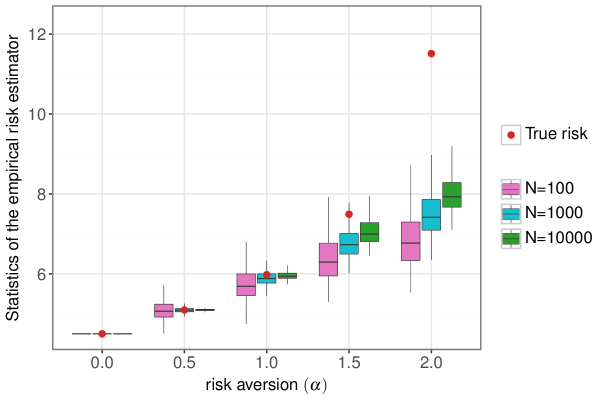
In an insurance pricing problem, the insurer aims to determine the minimum premium at which they can insure against the loss . Let risk aversion parameter of insurer be . Assuming full coverage for the losses , loss of the insurer if they charge a premium is a random variable given by . Thus, minimum premium at which the insurer insures the risk should be such that the entropic risk of the insurer from insuring is at most equal to , i.e., . On rearranging the terms, we can show that the minimum premium equals the entropic risk associated with the loss , . Suppose that the loss follows a distribution (see Fu and Moncher,, 2004; Bernard et al.,, 2020) with shape parameter and scale parameter . The moment-generating function of -distributed random variable is known in closed form which allows us to analytically compute the optimal premium
Suppose an insurer has access to samples of the losses which are generated from a -distribution. We use empirical distribution over samples to estimate the entropic risk for different risk averse parameters, . Figure 1 presents statistics of the distribution of the empirical risk estimator as a function of and . We can see that more risk-averse insurers significantly underestimate the risk of the loss and thus the premium to impose on the insuree. Furthermore, the slow convergence of sample mean to the true mean for heavy tailed random variables is a well-known phenomenon (Catoni,, 2012; Lugosi and Mendelson,, 2019). Even when the underlying distribution of is light-tailed, can be heavy-tailed (Nair et al.,, 2022). For instance, is a lognormally distributed when is Gaussian random variable.
The contribution of this paper is to propose a scheme to correct for the bias of the empirical entropic risk estimator, that is, find bias correction term that depends on a distribution fitted to the data so that
| (4) |
We show that almost surely with . This suggests that, with an infinite number of samples, it is possible to fit a distribution to the data using MLE and correct the bias. However, with limited number of samples, fitting a distribution using maximum likelihood criteria can lead to estimation errors and we will show later empirically that the underestimation problem persists. Instead, we provide two procedures to learn ”bias-aware” distributions that take into account the bias due to the tail events. The first one involves a distribution matching technique that mimics the bias in the samples, and the second one fits an extreme value distribution to the tails of the data.
Going beyond the estimation of entropic risk, we study the entropic risk minimization problem. Solving the sample average approximation (SAA) of the entropic risk minimization problem is known to produce a second source of bias, also known as the optimizer’s curse (Smith and Winkler,, 2006). Distributionally robust optimization (DRO) is widely used to address the optimistic bias of SAA policies because the decision-maker is protected against perturbations in the empirical distribution that lie in a distributional ambiguity set. Most of the literature on DRO with the Wasserstein ambiguity set assumes that the random variables involved in the expectation operator have light tails, a condition that is not satisfied for the entropic risk measure. It is well-known that worst-case loss in a DRO problem with type-p Wasserstein ambiguity set is finite if and only if the loss function satisfies a growth condition (Gao and Kleywegt,, 2023). Thus, the worst-case entropic risk can be shown to be unbounded for type-p Wasserstein ambiguity set with . So, we introduce a distributionally robust entropic risk minimization problem with type- Wasserstein ambiguity set and cast it into a finite-dimensional convex optimization problem for piecewise concave loss functions.
To tune the radius of the ambiguity set, a typical approach is to use K-Fold cross validation (CV). We use our bias correction procedure to estimate the validation performance of decisions. This leads to orders of magnitude improvement in out-of-sample entropic risk in terms of optimality gap compared to the “traditional” K-Fold procedure that chooses the radius of distributional ambiguity set based only on evaluating the decision on the validation loss scenarios.
Our contributions can be described as follows:
-
1.
On the theoretical side, we propose a strongly asymptotically consistent bootstrapping procedure to debias the empirical entropic risk estimator. Our main contribution lies in developing two bias-correction methods to mitigate the underestimation of the entropic risk in the finite sample case. In the first step, both methods fit a distribution to the samples to capture the bias in the samples. In the second step, bootstrapping is used to estimate the bias. Our methods could be of independent interest for debiasing more general risk measures.
-
2.
Our distributionally robust entropic risk minimization problem with a type- Wasserstein ambiguity set has bounded worst-case losses. We obtain its tractable robust counterpart for piecewise concave loss functions using Fenchel duality and provide conditions under which the optimal risk from the the DRO problem converges to the true optimal risk.
-
3.
On the application side, our work contributes toward data-driven designing of insurance premium pricing and coverage policies. To the best of our knowledge, this is the first time that a distributionally robust version of the well-known risk-averse insurance pricing problem is introduced in the literature. Our model takes into account the different risk aversion attitudes of the insurer and homeowners as well as the systemic risk associated with catastrophe events.
The paper is organized as follows. Section 2 surveys the literature on three related topics, estimating risk measures, correcting optimistic bias associated with solving SAA problem, and catastrophe insurance pricing. Section 3 discusses the properties of entropic risk measure. Section 4 provides a bias correction procedure to mitigate the underestimation problem. In Section 5, we study the entropic risk minimization problem using the DRO framework. In Section 6, we introduce the distributionally robust insurance pricing problem and provide numerical results. Finally, conclusions are given in Section 7.
Notations:
denotes the set of integers . denotes the dual norm of . is the Dirac distribution at the point .
2 Literature Review
2.1 Risk estimation
Quantitative risk measurement often relies on precise estimation of risk measures commonly used in finance and actuarial science (McNeil et al.,, 2005). Calculating risk for multidimensional random variables can be challenging due to the need for complex integrals, often approximated using Monte Carlo simulation. When the underlying distribution isn’t directly accessible and only limited samples are available, Monte Carlo-based risk estimators tend to underestimate the actual risk. Kim and Hardy, (2007) addressed this by using bootstrapping to correct bias in Value at Risk (VaR) and Conditional Tail Expectation (CTE) estimates, with Kim, (2010) extending this approach to general distortion risk measures. Bootstrapping involves sampling with replacement from the empirical distribution, calculating the statistic, and averaging the outcomes over multiple iterations. However, bootstrap estimates still tend to underestimate risk in finite samples due to the lack of extreme tail scenarios (see Figure 4). In contrast, our bootstrapping procedure draws samples from a ”bias-aware” fitted distribution that better accounts for tail scenarios.
Several approaches have been proposed in the literature for estimating tail risks. Lam and Mottet, (2017) introduce a distributionally robust optimization based method to construct worst-case bounds on tail risk, assuming the density function is convex beyond a certain threshold. Extreme Value Theory (EVT) is commonly used to estimate tail risk measures, such as CVaR, by fitting a Generalized Pareto Distribution to values exceeding a threshold. Troop et al., (2021) develop an asymptotically unbiased CVaR estimator by correcting the bias in the estimates obtained via maximum likelihood. While these methods focus on upper-tail risk, they are not directly applicable to the entropic risk measure. Instead of fitting an extreme value distribution, we utilize a parametric two-component Gaussian Mixture Model (GMM), which provides a closed-form expression for the entropic risk and captures both the mean and the tails of the data.
One related field of research is to derive concentration bounds on the risks estimates depending on whether the random variable is sub-gaussian, sub-exponential or heavy-tailed. For optimized certainty equivalent risk measures that are Hölder continuous, L.A. and Bhat, (2022) link estimation error to the Wasserstein distance between the empirical and true distributions, for which concentration bounds are available. While the Central Limit Theorem (CLT) ensures asymptotic convergence of the sample average to the true mean, this guarantee doesn’t always hold for finite samples unless the tails are Gaussian or sub-Gaussian (Catoni,, 2012; Bartl and Mendelson,, 2022). Robust statistics literature offers alternative estimators, like the median-of-means (MoM) estimator (Lugosi and Mendelson,, 2019), which ensure the estimator is close to the true mean with high confidence. However, these approaches differ from our focus, which is on constructing estimators with minimal bias.
2.2 Correcting optimistic bias
Our work on entropic risk minimization relates to correcting the optimistic bias of SAA policies to achieve true decision performance (Smith and Winkler,, 2006; Beirami et al.,, 2017). SAA is analogous to empirical risk minimization in machine learning, where the goal is to minimize empirical risk. Methods like DRO, hold-out, and K-fold CV are used to correct this bias. These approaches involve partitioning data into training, validation, and test sets, and then selecting the hyperparameter that results in smallest validation risk (Bousquet and Elisseeff,, 2000). Our hyper-parameter selection employs the debiased validation risk.
Several approaches have been proposed to correct the bias of SAA in linear optimization problems, assuming the true data distribution is Gaussian. Ito et al., (2018) propose a perturbation method to obtain an asymptotically unbiased estimator of the true loss, generating parameters around the true one under the assumption of Gaussian error. Similarly, Gupta et al., (2022) provide a procedure to debias the in-sample performance of affine policies under a Gaussian assumption. However, extending these methods to our non-linear problem is challenging, and our model isn’t limited to Gaussian distributions.
In Siegel and Wagner, (2023), the authors analytically characterize the bias in SAA policies for a data-driven newsvendor problem, providing an asymptotically debiased profit estimator by leveraging the asymptotic properties of order statistics. Iyengar et al., (2023) introduce an Optimizer’s Information Criterion (OIC) to correct bias in SAA policies, generalizing the approach by Siegel and Wagner, (2023). However, OIC requires access to the gradient, Hessian, and influence function of the decision rule, which can be challenging to obtain in general constrained optimization problems. Moreover, the form of optimal policy is known for risk-neutral newsvendor problems but not for entropic risk minimization problems.
2.3 Insurance pricing
The design of insurance contracts has been widely studied since the foundational work of Arrow (Arrow,, 1963, 1971). Under the assumption that premiums are proportional to the policy’s actuarial value, it has been shown that an expected utility-maximizing policyholder will choose full coverage above a deductible. Various extensions of Arrow’s model have been proposed to account for the risk aversion of both the insured and the insurer, using criteria such as mean-variance (Kaluszka, 2004a, ; Kaluszka, 2004b, ), Value at Risk (VaR), and Tail VaR (Cai et al.,, 2008). Bernard and Tian, (2010) incorporate regulatory constraints on the insurer’s insolvency risk through VaR. Cheung et al., (2014) extend these models to multiple policyholders with fully dependent risks (comonotonicity), where the insurer utilizes convex law-invariant risk measures. Bernard et al., (2020) further explore different levels of dependence among policyholders, with both insurers and policyholders valuing terminal wealth using exponential utility functions. However, these studies typically assume that the loss distribution is known. We extend the model proposed by Bernard et al., (2020) to account for ambiguity regarding the true loss distribution when only a limited number of samples are available.
3 Properties of entropic risk measure
The entropic risk measure is a convex-law invariant risk measure, thus satisfying the following definition.
Definition 1
Let denote the space of real-valued measurable functions, such that , where and is a probability space. A functional is a convex law-invariant risk measure if
-
for all and and .
-
if almost surely (a.s.) for all .
-
for and for all .
-
if for all .
Condition , cash-invariance property, states that is the minimum amount that should be added to a risky position to make it acceptable to a regulator. Condition , ensures monotonicity, meaning lower losses are preferable. Condition , convexity, ensures that diversification reduces risk. Lastly, condition , law invariance, states that two random variables with the same distribution should have equal risk.
To ensure that the mean and variance of are finite, we make the following assumption:
Assumption 1
The tails of are exponentially bounded:
for some and .
Assumption 1 further restricts the space of loss functions in Definition 1. We consider loss functions for which Assumption 1 holds. Although Assumption 1 might appear restrictive, intuitively we cannot expect to correct the bias with finite number of samples if the true risk is . For many light tail distributions, like the GMM, Assumption 1 holds, thus entropic risk is finite for any finite risk aversion parameter .
Lemma 1
Under Assumption 1, and .
4 Bias correction using bias-aware bootstrapping
In this section, we introduce our proposed estimators designed to address the underestimation problem associated with the empirical entropic risk estimator, . The true bias is given by . Since the true distribution is unknown, the exact bias cannot be determined. A typical approach in the literature to estimate the bias is using bootstrapping which samples repeatedly from the empirical distribution. Such bootstrapping procedure has been shown to be weakly consistent (DasGupta,, 2008), however, it exhibits significant bias for small sample sizes. In this paper, we propose a modification to the bootstrap algorithm, namely, we first fit a distribution using the i.i.d. loss scenarios and then repeatedly sample from , instead of resampling from the empirical distribution. We will demonstrate that fitting a distribution is crucial step in reducing bias. However, merely fitting a distribution using maximum likelihood estimation (MLE) does not fully resolve the underestimation issue, which is why we introduce bias-aware procedures to better fit the data, see Sections 4.1 and 4.2.
Let a sample capture the loss associated with the uncertain parameter . Similar to Assumption 1, the following assumption ensures that the mean and variance of are finite.
Assumption 2
Suppose that the tails of are almost surely uniformly exponentially bounded. Namely, with probability one with respect to the sample and the fitting procedure of , there exists some and some such that satisfies Assumption 1 for all .
This assumption is not limiting since we have assumed that satisfies this assumption under . In practice, this assumption could be satisfied by properly defining the set of models used to fit to the observed realizations of .
Next we introduce the necessary notation to describe our estimation procedure. Let denote the entropic risk for the distribution . Let represent the empirical distribution of values drawn i.i.d. from the estimated distribution , and denote the corresponding empirical entropic risk. Notice that since was estimated using loss scenarios, it is itself random, thus and are random variables as well. The proposed estimator for the bias of the entropic risk is given by
| (5) |
Algorithm 1 provides an estimate for the bias. Given loss scenarios , the algorithm first estimates , and then repeatedly samples i.i.d. scenarios from to form the empirical distribution . For each of the repetitions, it estimates the entropic risk, denoted by the sequence . Finally, the bias is estimated through . Note that as increases, the resampling (simulation) error in the bootstrap estimate decreases, and the bootstrap estimate converges to the true estimate .
In the next theorem, we show that the bias-adjusted empirical risk given by is an asymptotically consistent estimator of the true risk , meaning that as the number of training samples , the bias-adjusted empirical risk almost surely converges to the true entropic risk.
Theorem 1
The estimator is strongly asymptotically consistent.
The proof involves two key steps: The first step is to establish that the empirical entropic risk converges to the true risk almost surely. This is achieved by using the strong law of large numbers and the continuous mapping theorem. The strong law of large numbers ensures that the average of exponentiated losses converges almost surely to its expected value, and the continuous mapping theorem extends this convergence to the logarithmic transformation involved in the entropic risk, leading to the almost sure convergence of the empirical risk to the true risk. The second step involves showing that the bias term, converges to zero almost surely. This is accomplished by showing that the bias, calculated under any sequence of fitted distributions that satisfy Assumption 2 can be made arbitrarily small for sufficiently large . We show that the almost sure convergence of bias to zero is equivalent to proving that the median of a random variable representing the ratio of empirical and true risk under converges to almost surely. To establish this, Chebyshev’s inequality is used rather than the CLT, as it applies for any finite . By setting the upper tail probability to 25% in the Chebyschev’s inequality, the median of is bounded within an interval around which becomes smaller as increases. Consequently, the median of converges to almost surely. Thus, for any sequence of distributions which satisfy Assumption 2, the bias converges almost surely to zero.
Our approach does not rely on asymptotic or parametric (Gaussian, for instance) assumptions made in the literature to correct the bias. Many bias correction methods assume that the estimator’s error is asymptotically normally distributed and linear, with the error term diminishing faster than one over the square root of the sample size. This allows for deriving a bias correction term (see Iyengar et al., (2023)). However, these corrections hold only asymptotically. In contrast, our method is motivated by addressing the underestimation issue in finite samples. While bias estimated via bootstrapping can be added to the empirical risk to construct a strongly asymptotically consistent estimator, a limited sample size can introduce statistical errors when using MLE to estimate the distribution, leading to inaccurate bias corrections.
Among the options for choosing the distribution , we utilize a where denotes the weights of the mixtures, and and denote the means and standard deviations of the mixtures, respectively. There are many advantages for using GMM: GMMs are universal density approximators, meaning they can approximate any smooth density given sufficient data, the moment-generating function of a random variable exists for all , and thus the entropic risk can be obtained in closed form. This eliminates the need to estimate the entropic risk through simulation, which can be particularly beneficial when the risk aversion parameter is large, as this would otherwise require a large number of samples for accuracy.
The natural approach for fitting a GMM is to use MLE, typically achieved via the Expectation-Maximization algorithm (Dempster et al.,, 1977). In the following example, we demonstrate that our bootstrapping procedure, which fits a GMM using the Expectation-Maximization algorithm, still underestimates the true risk.
Example 2
Consider the problem of estimating the entropic risk of a random variable that follows a Gaussian mixture model with two components , , , and To obtain Figure 2, we draw i.i.d. samples from where . The true bias correction is obtained by first computing the true entropic risk and then subtracting the expected empirical entropic risk obtained by bootstrapping with repetitions. We fit a GMM to the samples using the Expectation-Maximization algorithm and use the same bootstrapping approach to estimate the bias. The boxplots are plotted for 100 repetitions of this experiments. Fitting a GMM by MLE still underestimates the true bias for finite number of samples. Also, we can observe that as the number of training samples increase, the bias estimated by fitted GMM converges toward .
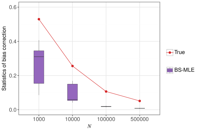
Bootstrapping corrects bias in empirical entropic risk estimator if the bias in i.i.d. samples from the fitted distribution matches that of the true distribution . We can satisfy this condition if we can correctly estimate the true underlying distribution . Although GMM is a universal approximator of density, MLE with limited samples introduces statistical errors in parameter estimation. This motivates the use of a “bias-aware” distribution matching algorithm (described in the next section) for learning a GMM , whose i.i.d. samples capture the bias present in i.i.d samples from the true distribution . This approach is inspired by “decision-aware” learning of estimators for contextual optimization problems (Elmachtoub and Grigas,, 2021; Donti et al.,, 2017; Sadana et al.,, 2024) where one trades statistical accuracy for decision quality.
4.1 Entropic Risk Matching
In this section, our goal is to learn a GMM whose samples mimic the bias in the loss scenarios. This bias corresponding to the learned GMM is estimated using bootstrapping and added to the empirical entropic risk to mitigate the underestimation problem.
The objective of Algorithm 2 is to learn the parameters of a GMM, denoted , which minimize the Wasserstein distance between two distributions. The first distribution is one of the entropic risk derived from i.i.d. samples from , while the second distribution is the distribution of the entropic risk computed using a subset of the observed loss scenarios from the true distribution .
Initially, the algorithm starts by partitioning the given loss scenarios, denoted as into bins, where represents the loss corresponding to the random variable . Each bin contains loss scenarios. For each bin, the entropic risk is computed, producing an empirical distribution of the empirical entropic risk based on the observed data. This empirical distribution represents the entropic risk derived directly from the true loss scenarios.
Next, we fit a GMM, referred to as to the loss scenarios in . The GMM is fitted using the Expectation-Maximization algorithm, which provides initial estimates of the model parameters . These parameters include the mixing weights , means , and standard deviations for each component of the GMM. To compare the model-based distribution of entropic risk to the empirical distribution of entropic risk, samples are generated from the GMM. Specifically, i.i.d. samples are drawn from the initial GMM with parameters , and these samples are divided into bins. The entropic risk is computed for each bin, producing a model-based distribution of the entropic risk. This distribution is derived from the GMM and is used to assess how well the GMM replicates the risk profile of the true data.
The next step is to compare the empirical distribution with the model-based distribution using the Wasserstein distance, denoted as , where the Wasserstein distance is defined as follows:
| (6) |
where is a joint distribution of and with marginals and , respectively. This distance quantifies the discrepancy between the two distributions. The algorithm iteratively adjusts the GMM parameters to reduce this distance, using gradient descent to update the parameters at each iteration. Specifically, the parameters are updated according to:
where is the step size. Algorithm 6 generates “differentiable samples” from the GMM, , which are then used to compute the Wasserstein distance. This enables the calculation of the gradients of the Wasserstein distance with respect to (see Appendix B).
After each update, the parameters are projected back into the feasible region for a valid GMM. This ensures that the mixing weights remain valid probabilities (which is achieved using a softmax function), and that the standard deviations are positive (enforced by taking the maximum of and ).
The iterative process continues until the Wasserstein distance falls below a predefined convergence threshold , or until a maximum number of iterations is reached. Once convergence is achieved, the final GMM, , is returned as the learned model that best approximates the entropic risk distribution of the true data. The number of components in the GMM is selected by choosing the value that minimizes the Wasserstein distance. By iteratively adjusting the parameters and refining the number of components, the algorithm ensures that the learned GMM closely matches the distribution of entropic risk from the original data.
Once we learn the distribution using Algorithm 2, we use it in Algorithm 1 to estimate the bias
Even though computing the Wasserstein distance between distribution of losses has a worst-case complexity (Kolouri et al.,, 2018), there is a significant total cost associated with the gradient descent procedure described in Algorithm 2. In the next section, we provide a semi-analytic procedure to learn a two-component GMM that can account for the tail scenarios.
4.2 Matching the extremes
This section aims to approximate the tails of the true underlying distribution in order to improve the estimation of the entropic risk, which depends on the full distribution but is particularly sensitive to the tails. Our approach uses the distribution of tails of normal distribution to approximate the distribution of the maxima of the data, motivated by both extreme value theory and the need for an analytical solution.
Consider a random variable . Given i.i.d. samples of drawn from , the maximum of the samples is denoted as . According to the Fisher–Tippett–Gnedenko theorem, the distribution of a (normalized) maxima converges to a non-degenerate distribution :
| (7) |
where and are normalizing sequences of scale and location parameters, respectively, that ensure the limit exists. The limit distribution belongs to one of three extreme value distributions–Weibull, Fréchet or Gumbel distribution–depending on the tails of (Haan and Ferreira,, 2006).
While the entropic risk depends on the entire distribution of losses, its sensitivity to extreme values makes it important to approximate the tail behavior accurately. However, rather than directly fitting an extreme value distribution to the empirical tails, we approximate the distribution of the maxima by fitting a normal distribution and use this to construct a GMM. This approach is motivated by the fact that GMM provides a closed-form analytical solution for the entropic risk, making computations efficient in the bootsrapping step.
The key idea is not to fit a normal distribution to the data itself but rather to match the distribution of the maxima of i.i.d samples drawn from a normal distribution with the distribution of maxima of i.i.d samples drawn from the empirical data. This approach is inspired by the Fisher–Tippett–Gnedenko theorem, which indicates that the distribution of the normalized maxima will converge to one of the three possible extreme value distributions. By using a normal distribution, we strike a balance between capturing the tail behavior and retaining analytical tractability.
To empirically estimate the distribution of maxima from the observed data, we use the block maxima method, commonly applied in extreme value analysis (Haan and Ferreira,, 2006). The algorithm for fitting a normal distribution whose tails match those of the loss scenarios is outlined in Algorithm 3. First, we divide the scenarios in the set into bins, each of size and then compute the maximum within each bin. Let denote the cumulative distribution function (cdf) of the maxima.
The distribution of the maxima of i.i.d samples from a normal distribution is given by where is the cdf of a normally distributed random variable with mean and . We find the parameters of the normal distribution by matching the 50th and 90th quantiles of to the corresponding quantiles of :
where the -th quantile for is given by . Solving the above two equations in gives an approximate distribution for the tails of the underlying distribution, which depends on the true distribution, the total number of samples , and the number of bins .
To balance the trade-off between the number of bins and the sample size in each bin, we set , which is a reasonable compromise. A large number of bins provides more independent realizations, reducing estimation bias, while a sufficiently large sample size in each bin ensures that the maxima accurately represent the extremes of the distribution.
For analytical tractability in risk estimation, we restrict the model to a two-component GMM with equal weights for each component. The GMM’s mean is set to be the mean of the data , and the variance of one component is set to zero, resulting in a GMM with one component as a Dirac delta distribution and the other as a normal distribution . These components satisfy the condition: .
The GMM learned using Algorithm 3 is used for bias correction through bootstrapping, similar to the entropic risk matching approach.
4.3 Numerical illustrations
In this section, we review several methods from the literature for estimating entropic risk and show through numerical examples that they significantly underestimate it.
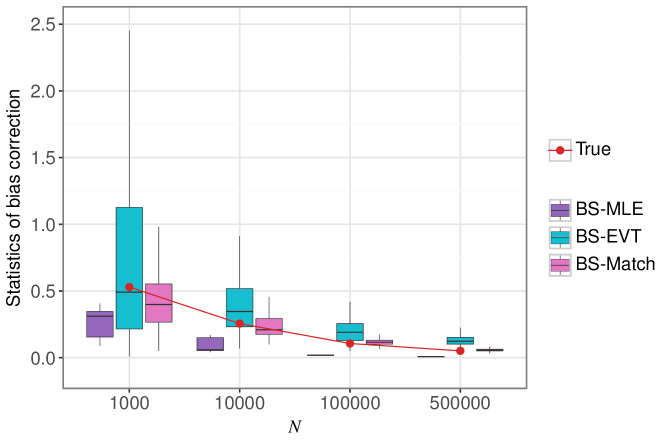
We have already shown that naively fitting a GMM underestimates the true risk. In Figure 3, using the setup from example 2, we demonstrate that our methods (BS-Match and BS-EVT) help mitigate this underestimation, even with finite samples. For , the bias correction decays at a rate similar to the bootstrapped true bias estimate. However, EVT tends to overestimate the correction.
The next example illustrates that several approaches from the literature underestimate the true entropic risk significantly.
Example 3
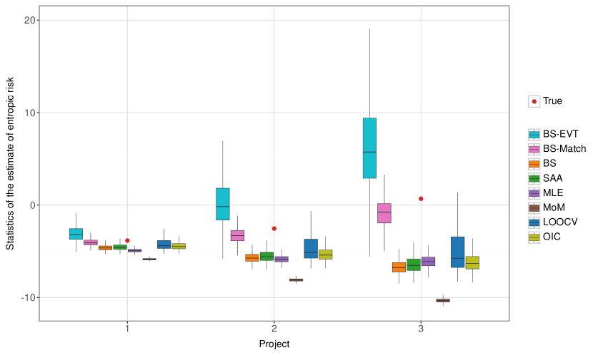
Consider a project selection problem with three projects. Let with . The expected value of is and standard deviation is . Suppose the losses associated with the three projects are given by , and , respectively. Let the risk aversion parameter be . The true entropic risk computed as: . To evaluate the estimates of entropic risk, we draw instances with a sample size of from the .
SAA:
We compute the empirical entropic risk using the SAA for each project, resulting in the boxplots shown in Figure 4. The SAA method tends to underestimate the true risk because it fails to account adequately for tail events that have a low probability but significant impact on the entropic risk.
We can construct estimators for the entropic risk using leave-one-out cross-validation (LOOCV) and the Optimizer’s Information Criterion (OIC). Both approaches are based on an alternative representation of the entropic risk as an optimized certainty equivalent risk measure (Ben-Tal and Teboulle,, 1986):
| (8) |
where . The optimal solution is given by .
LOOCV:
The LOOCV estimator provides an alternative way to estimate entropic risk. For each sample , we solve the SAA problem without , obtaining
where . The LOOCV estimator is then given by
Since is a feasible solution of the minimization problem in (8) for all , we have for each . Thus, . We have show that is positively biased. Even though LOOCV estimators overestimate the true entropic risk, we can see in Figure 4 that the estimator has a skewed distribution where the entropic risk is below the true risk for more than times.
OIC:
MoM.
The median-of-means (MoM) estimator partitions the loss scenarios into blocks, computes the mean within each block, and then takes the median of these means. This estimator is robust to outliers and is widely studied in the context of robust statistics (Lugosi and Mendelson,, 2019).
MLE:
We fit a GMM to the loss scenarios using the Expectation-Maximization algorithm, a popular method for maximizing the likelihood of the GMM parameters. However, the GMM fitted using MLE often underestimates the true entropic risk in the finite sample setting.
BS:
We apply the traditional bootstrapping approach (BS) by sampling 5000 observations with replacement from the empirical distribution, computing the empirical entropic risk, and repeating this procedure 1000 times. We report the statistics of the average entropic risk across these repetitions.
We can see in Figure 4 that the estimators discussed above, including LOOCV, significantly underestimate the true entropic risk in most of the randomly generated instances for projects 2 and 3. On the other hand, our proposed estimators (BS-EVT and BS-Match) are able to mitigate the underestimation problem. Specifically, BS-EVT overestimates the entropic risk and BS-Match reduces the bias significantly compared to SAA.
5 Distributionally Robust Optimization
In data-driven optimization, the objective is to solve the following problem:
| (9) |
where denotes the set of all feasible decisions, denotes a decision, denotes the uncertain parameter, , and the loss function depends on both and . Let denote the optimal decision obtained by solving (9).
For the optimal solution of problem (9) to be well defined, we make the following standard assumptions:
Assumption 3
We assume that
-
1.
is convex in for almost surely every .
-
2.
is continuously differentiable in for almost surely every .
-
3.
For all , the tails of are exponentially bounded:
for some and .
The true underlying distribution is typically not known in practice, so one instead uses the samples to solve the SAA of (9):
| (10) |
where the empirical distribution, , of the scenarios replaces the true distribution. Under fairly mild assumptions, the optimal risk for the SAA problem denoted by converges to the true risk , see Lemma 2 in Appendix A. Thus, SAA approach is typically used to solve entropic risk minimization problems (Chen and Sim,, 2024); refer to Shapiro et al., (2009) for a comprehensive overview of SAA approach for stochastic programming.
In the limited data setting, the risk produced by solving problem (10) underestimates the true risk due to overfitting on the empirical distribution. Distributionally robust optimization (DRO) is one of the approaches to mitigate the optimistic bias of SAA by robustifying decisions against perturbations in the empirical distribution (Wiesemann et al.,, 2014; Delage and Ye,, 2010; Rahimian and Mehrotra,, 2022). It is assumed that nature perturbs the nominal distribution, e.g., empirical distribution, in a distributional ambiguity set so as to maximize the entropic risk of the decision maker, while decision maker aims to minimize the worst-case risk resulting in the following min-max problem:
| (11) |
where contains all distributions that are at a “distance” away from the empirical distribution . Here, is a parameter that controls the size of the ambiguity set and is chosen by the decision maker.
In the literature, different ambiguity sets have been considered with the Kullback Leibler (KL)-divergence (Hu and Hong,, 2012) and Wasserstein ambiguity sets (Mohajerin Esfahani and Kuhn,, 2018) being the most commonly used (Rahimian and Mehrotra,, 2022). For KL-divergence-based ambiguity sets, the worst-case distribution is absolutely continuous with respect to the empirical distribution and does not contain distributions with support on points for which the empirical distribution is not supported. This makes the KL-divergence-based ambiguity set unsuitable for our problem with unbounded support. On the other hand, type- Wasserstein ambiguity set with results in unbounded worst-case loss when used in problem (11) (see Theorem 6 in Appendix B):
The type- Wasserstein distance is defined as follows:
where is a joint distribution of and with marginals and , respectively, ess.sup denotes essential supremum, and denotes the -norm with . Then, type- Wasserstein ambiguity set of radius , can be defined as follows:
| (12) |
Let the ambiguity set be defined as:
| (13) |
where is a Dirac measure at . From Bertsimas et al., (2023), problem (11) can be equivalently written as follows:
| (14) |
Since is a monotonic function, problem (14) is equivalent to:
| (15) |
Thus, DRO problem in (11) with type- Wasserstein ambiguity set is equivalent to the robust optimization problem (15) with one uncertainty set associated with each scenario and nature can perturb each scenario in the ball . Thus, the worst-case loss is always bounded for finite radius of the uncertainty set.
Consider the loss function . The function is increasing in . Thus, its supremum over the set is attained at the boundary of this set. This leads to the result:
| (16) |
where the second equality follows from the definition of the dual norm and denotes the dual norm of . On combining with the objective function in (15), we obtain:
So, with a linear loss function, problem (14) is equivalent to the regularized risk-averse SAA problem:
| (17) |
For piecewise concave loss functions, Theorem 2 gives an equivalent reformulation of the DRO problem as the finite dimensional convex optimization problem using Fenchel duality.
Theorem 2
Let where is a concave function in for each and . Then, the DRO problem (14) with type- Wasserstein ambiguity set is equivalent to
| (18a) | ||||
| (18b) | ||||
where is the partial concave conjugate of .
In Appendix A, we provide reformulations of distributionally robust newsvendor and regression problems as exponential cone programs. However, robustifying the SAA problem does not necessarily change the optimal decision, as highlighted in the following remark:
Remark 1
By translation invariance of entropic risk measure, minimizing the worst-case entropic risk of loss function that is separable in and is equivalent to solving the SAA problem.
Furthermore, by assuming that the tails of loss are exponentially bounded as in Assumption 3 with , we can ensure that the rate of convergence of risk of SAA problem to the true risk is for sufficiently large (see Lemma 2 in the Appendix B). This also ensures the convergence of to in probability (see Theorem 5 in Appendix B).
5.1 Calibrating the radius
In this section, we describe the procedure for calibrating the radius parameter . Let be a grid of potential radius values, including . For each radius , Algorithm 4 applies the K-fold cross-validation algorithm to generate the validation scenarios . Specifically, we partition the dataset into folds, where each fold is denoted by .
The model is trained on all but one fold, , and the loss is evaluated on the remaining fold, , to produce validation losses. To this end, we solve (18) over dataset to find the optimal decision . The loss of decision is then computed on each sample, , in the validation fold . This process is repeated for all folds and the resulting loss scenarios are aggregated to form a set of size equal to training sample size .
Algorithm 5 calculates the entropic risk across the scenarios in for each radius . A GMM is then fitted to the scenarios in , and and bootstrapping is used to estimate the bias, which is added to to obtain the bias-corrected risk . This procedure is repeated over all radius and the optimal radius is chosen as the one minimizing . The GMM can be fitted using MLE, entropic risk matching (Match), or by matching the tails (EVT).
In contrast, traditional CV sets to for all . By Jensen’s inequality, this underestimates the true risk in the validation set, potentially leading to errors in radius selection. In Example 3, the projects can be seen as corresponding to different regularization parameters, with lower values of representing riskier projects. Traditional CV would select project 3, whereas our approach, based on bias-corrected estimators, selects project 1.
6 Distributionally robust insurance pricing
The International Panel on Climate Change (IPCC) advocates using financial instruments like catastrophe insurance to mitigate risks associated with rare, high-impact events such as floods, earthquakes, and wildfires. Such instruments are crucial for climate change adaptation (Linnerooth-Bayer and Hochrainer-Stigler,, 2015). These events have become more frequent due to climate change, making reliable risk estimation critical. However, the rarity of such events leads to limited data, which poses challenges for accurate risk assessment. High insurance premiums often deter homeowners from purchasing insurance, with demand typically spiking only after catastrophic events (Gallagher,, 2014). The correlated risks of floods, earthquakes, and wildfires can lead to significant payouts for insurers, limiting the availability of flood insurance in commercial markets. For instance, the US National Flood Insurance Program (NFIP) faces over $20 billion deficit (Marcoux and H Wagner,, 2023) due to underpriced premiums and low uptake, highlighting the need for optimal pricing that accounts for homeowners’ behavioral responses (Kousky and Cooke,, 2012).
We consider a model of insurance pricing with one risk-averse insurer and representative risk-averse homeowners, based on the framework introduced by Bernard et al., (2020). In their model, both the insurer and homeowners are assumed to be expected utility maximizers, with loss distributions and risk aversion parameters known to the insurer. We depart from these assumptions by only providing samples of the loss distribution to both the insurer and homeowners.
Let be the risk aversion of homeowner , and let the insurer’s risk aversion parameter be . The uncertain loss faced by homeowner is represented by . The insurer offers a policy to homeowner where the indemnity function specifies the coverage provided, and is the premium paid by the homeowner.
If homeowner rejects the insurance policy, the entropic risk is .
If homeowner accepts the insurance policy, the entropic risk is .
Let denote each homeowner’s loss distribution . The insurer’s demand response model assumes that homeowner will accept the insurance policy if the empirical entropic risk with insurance is less than the entropic risk without insurance:
where is the empirical distribution of the losses faced by homeowner . This model assumes that the decision to accept the insurance policy is based solely on the empirical distribution of the losses. Alternative demand response models could be considered, allowing for a corresponding analysis to be conducted.
The entropic risk of the insurer is given by:
Since the insurer does not know the true distribution , and the marginal distribution are also unknown to the homeowners, decisions based on the SAA can be optimistically biased. To address this, the insurer solves the following distributionally robust insurance pricing problem, which minimizes the worst-case entropic risk:
| (19a) | |||||
| subject to | (19b) | ||||
where lies in the type- Wasserstein ambiguity set given in (12). From Theorem 2, the above problem can be reformulated as the following regularized exponential cone program:
| (20) | |||||
| subject to | (21) | ||||
6.1 Numerical Experiments
To illustrate our model and algorithm using numerical experiments, we consider homeowners with risk aversion parameters . For all methods, except SAA and Opt, we use K-fold cross-validation procedure given in Algorithm 4 with to construct the validation dataset of loss scenarios. Let denote the empirical entropic risk of loss scenarios in for a given radius . The selection of varies across methods as follows:
-
•
Traditional CV approach: The radius is chosen based solely on .
-
•
BS-EVT: A two-component GMM is fitted to the loss scenarios in set and the radius is selected based on bias-corrected values of
-
•
BS-Match: Entropic risk matching is employed to fit a GMM to the loss scenarios in and the radius is selected based on bias-corrected values of .
-
•
Opt: The radius is calibrated based on the entropic risk over the test data-points.
After choosing the radius for each model, we find the optimal decision by solving SAA problem using all the training samples. The distribution of losses is modeled using a Gaussian copula with Gamma-distributed marginals and a correlation coefficient across homeowners. Let denote the positive-definite covariance matrix:
where is a vector of all ones and is the identity matrix. Samples are generated by first drawing a multivariate normal vector , and transforming element-wise using the standard normal cdf, . Finally, the losses are sampled from a Gamma distribution:
where is the inverse cdf of the Gamma distribution, and and are its shape and scale parameters, respectively.
The boxplots are obtained for repeated experiments, each experiment done by sampling training samples from the Gaussian copula. The regularizer is chosen from a set containing and equally-spaced values in the interval on the log scale. Using the values of correlation coefficient and parameters of marginal distribution, we sample i.i.d. data points from the Gaussian copula that are used to evaluate the out-of-sample performance.
Homeowners have different marginal distribution.
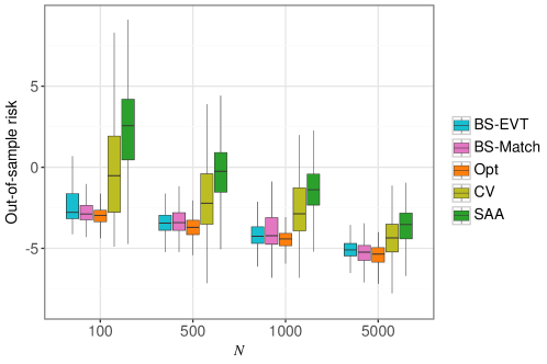
In this experiment, the scale and location parameters of the -distributed marginals of 5 homeowners are given by , , , , and , respectively. The correlation coefficient is set to .
Figure 5 shows the variation in the out-of-sample entropic risk with the number of training data-points. It is evident from the figure that our models, BS-EVT and BS-Match,outperform the traditional CV method and the SAA, resulting in a lower out-of-sample entropic risk. This suggests that both the EVT and entropic risk matching based approaches offer better generalization and robustness compared to standard empirical risk minimization techniques when applied to insurance risk estimation under limited training data scenarios.
Homeowners have same marginal loss distribution
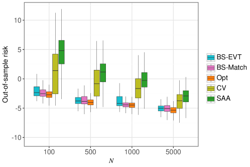
To analyze the impact of the training sample size, , and the correlation coefficient, , on the out-of-sample risk and premium per unit expected coverage, we assume the marginal distribution of loss across households follows .
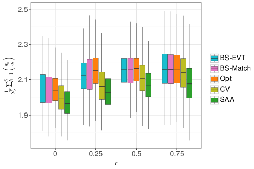
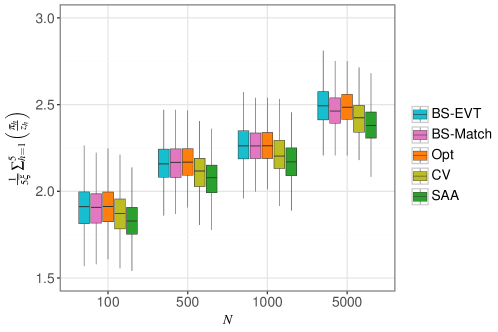
As depicted in Figure 6, out-of-sample risk decreases with increase in the number of training data points. This decrease occurs because the premium per unit coverage better reflects the true risk exposure of the homeowners as shown in Figure 7. Consequently, with larger values of , the insurer can extract higher premium from the homeowners for the same coverage level. The average out-of-sample loss, denoted as in Figure 7 remains constant across households.
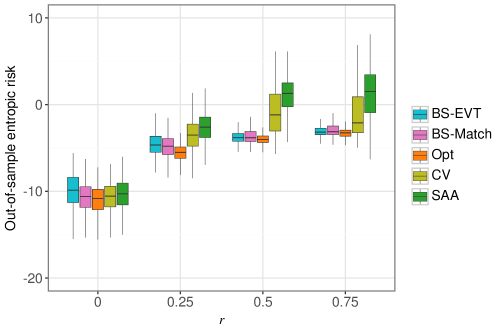
Figure 8 demonstrates that the out-of-sample entropic risk initially increases with the correlation coefficient , eventually stabilizing. A similar trend is observed in Figure 9 which shows the variation in the average premium per unit expected coverage across homeowners. This behavior can be attributed to the insurer setting higher premiums, potentially leading homeowners to opt out of insurance coverage.
7 Conclusions
In this paper, we propose two practical approaches to mitigate the bias inherent in the empirical entropic risk estimator, which arises when the empirical distribution is used in place of the true distribution in entropic risk calculations. We prove that the bias-corrected entropic risk estimator converges almost surely to the true risk. However, when a GMM is fitted using maximum likelihood estimation and the bias is estimated via bootstrapping, the bias-corrected estimator often underestimates the true risk in finite samples. Our proposed approaches address this underestimation problem by estimating the bias in samples drawn from a “bias-aware” GMM fitted to the data.
To address the optimistic bias associated with optimizing the entropic risk measure, we propose to use type- Wasserstein ambiguity sets in DRO models. This is because other type- Wasserstein ambiguity sets with lead to unbounded worst-case entropic risk for any decision. For piecewise-concave loss functions, we provide equivalent reformulations of DRO problems as finite-dimensional convex optimization problems using Fenchel duality. Additionally, we introduce a distributionally robust version of a well-known insurance pricing problem. Numerical experiments demonstrate that our bias correction procedures help identify the appropriate radius for the ambiguity set, resulting in premium pricing and coverage policies that achieve lower out-of-sample entropic risks when compared to cross-validation methods that do not account for bias in the validation scenarios.
Appendix A Proofs
A.1 Proof of Lemma 1
We have that:
We also have that:
Hence that
Similarly,
Hence,
A.2 Proof of Theorem 1
We want to show that almost surely. To do so, we will show that both and almost surely. Indeed, if both and almost surely, then we can use the fact that the sum of two convergent sequence converge to the sum of their limits to conclude that:
where the second inequality follows from the union bound.
Step 1: almost surely. Given that is finite (see Lemma 1) and each is i.i.d., the strong law of large numbers tells us that
| (22) |
Since is continuous over the strictly positive values, using the continuous mapping theorem (Van der Vaart,, 2000), we obtain:
Hence, almost surely.
Step 2: almost surely. We will show that almost surely by showing that almost surely.
Let’s consider any sequence that is uniformly exponentially bounded, with each element of the sequence satisfying Assumption 2. For each , we have
where . The second equality follows by the monotonicity of the exponential function, and the third equality follows by the definition of the entropic risk and the properties of the logarithm. Note that are drawn i.i.d. from .
To analyze the , we first study the mean and variance of . It is easy to see that , while the variance of can be bounded as follows,
where the second equality follows from the fact that the are i.i.d. The inequality follows since satisfy Assumption 2, thus Lemma 1 provides bounds for both and , resulting in the bound .
We next show that is bounded. To this end, consider the Chebyshev’s inequality
Substituting the bound for the , and setting which implies an upper tail probability bound of 25%, results in
where . Thus, we conclude that since otherwise it would imply that 50% of the probability is outside this interval (either on the right or the left), which would contradict the fact that the total probability outside the interval is below 1/4.
Finally, we show that as tends to infinity, converges to 1 almost surely. For any , there exists an such that for all , which implies .
A.3 Proof of Theorem 2
(15) is equivalent to
| (23a) | |||||
| (23b) | |||||
where . Since , we obtain:
| (24a) | |||||
| (24b) | |||||
The relative interior of the intersection of set and domain of is non-empty for all . So, we can use Fenchel duality theorem (Ben-Tal et al.,, 2015) to obtain
| (25) |
where , is the partial concave conjugate of and is the support function of , i.e.,
| (26) |
by the definition of the dual norm. We therefore obtain:
| (27) |
When the cost function is an inner product, i.e., and , we obtain
| (30) |
Thus, problem (27) reduces to:
| (31) | ||||
| (32) |
Replacing the epigraph variable , we obtain that the objective reduces as follows:
Corollary 3
For the newsvendor problem with the cost function given by , DRO with type- Wasserstein ambiguity set is equivalent to
| (33) |
Proof.
For the newsvendor problem, the cost function is given by . (23b) is equivalent to
| (34a) | |||||
| (34b) | |||||
| (34c) | |||||
where . Define and for which the partial concave conjugates are given by:
| (37) |
| (40) |
Corollary 4
For the regression problem with loss function given by , DRO with type- Wasserstein ambiguity set is equivalent to
| (41) |
Proof.
Appendix B Additional results
Lemma 2
Suppose that is compact, are i.i.d with distribution , and the loss function is Lipschitz continuous in with Lipschitz constant . Also, suppose that there exists a for which for all . Then, it can be shown that for any , there exists a constant , that is independent of for which,
| (51) |
for sufficiently large .
Proof. From the local lipschitz continuity of in for , we have:
| (52) |
where is the lipschitz constant. From the Mean Value Theorem, we obtain:
where and the first inequality follows from the Cauchy-Schwarz inequality and the second from (52). Since is a compact set, and there exists some for which , it follows from Theorem 3.2 in Jiang et al., (2020) that for any , there exists , independent of , such that
| (53) |
for sufficiently large . Denote by and by . From the concavity of , it follows that:
where the second inequality follows from . The above inequality implies that
On combining with (53), we obtain
| (54) |
Finally, we note that
On combining the above inequality with (54) and substituting , we obtain
Theorem 5
Suppose is Lipschitz in for all with Lipschitz constant , and assume the SAA solution’s entropic risk converges to the true risk at rate for sufficiently large . If the radius of the ambiguity set is , then the risk converges to the optimal risk in probability, i.e., for any , there exists a constant such that:
Proof. Since , the following inequality holds for all
Taking the minimum over on both sides of the above inequality, we obtain
To prove the other side of the inequality, we will use the lipschitz continuity of in for all :
where is the lipschitz constant. From Bertsimas et al., (2023), the following problems are equivalent
| (55) |
Then, it follows from the lipschitz continuity of and that
The above inequality implies that
Substituting in (55), we obtain:
From the above inequality, we can show that
where . Taking with , we obtain,
Using the triangle inequality, we have:
Therefore for , we have
Combining the above inequality with Lemma 2, we obtain
Since , we obtain
Theorem 6
-Wasserstein DRO with entropic risk measure results in unbounded loss if .
Proof. Let denote the worst-case expected utility for a given decision :
| (56) |
From Gao and Kleywegt, (Lemma 2, Proposition 2, 2023), the worst-case disutility is infinite with -Wasserstein ambiguity set since the loss function does not satisfy the growth condition: , for all and some constants , and for any . Next, we will prove that is unbounded for all implies that is unbounded for all by contradiction. Suppose that is bounded. Then such that
| (57) |
Since the above relation holds for all and is a monotonic function, we obtain:
This implies that is bounded, which contradicts the fact that is unbounded.
B.1 Influence function
A way to explain the underestimation effect of a finite sample can be seen when looking at the loss distribution through the influence function. The influence function measures the sensitivity of entropic risk to small changes in the data. The influence function of a statistic at a point for a distribution is given by
where is the Dirac distribution at the point . The influence function of entropic risk measure is given by
For entropic risk measure , for any support point can be obtained in closed form for -distributed loss as follows:
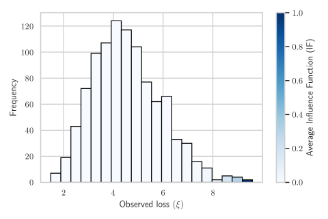
In Figure 10, we plot the histogram of loss values generated from the distribution. We compute the average IF over samples in each bin and darker shades represent higher (normalized) values of average IF. It can be seen that tail events have highest impact on the entropic risk but occur with very low probability. Therefore, these high impact scenarios are likely not to be included in a finite sample, resulting in the underestimation effect.
B.2 Bias correction using OIC
B.3 Differential sampling from GMM
References
- Arrow, (1963) Arrow, K. J. (1963). Uncertainty and the welfare economics of medical care. American Economic Review, 53:941–973.
- Arrow, (1971) Arrow, K. J. (1971). Essays in the Theory of Risk Bearing. Markham Publishing Co., Chicago.
- Artzner et al., (1999) Artzner, P., Delbaen, F., Eber, J.-M., and Heath, D. (1999). Coherent measures of risk. Mathematical finance, 9(3):203–228.
- Bartl and Mendelson, (2022) Bartl, D. and Mendelson, S. (2022). On monte-carlo methods in convex stochastic optimization. The Annals of Applied Probability, 32(4):3146–3198.
- Beirami et al., (2017) Beirami, A., Razaviyayn, M., Shahrampour, S., and Tarokh, V. (2017). On optimal generalizability in parametric learning. In Advances in Neural Information Processing Systems, volume 30. Curran Associates, Inc.
- Ben-Tal et al., (2015) Ben-Tal, A., den Hertog, D., and Vial, J.-P. (2015). Deriving robust counterparts of nonlinear uncertain inequalities. Mathematical Programming, 149(1):265–299.
- Ben-Tal and Teboulle, (1986) Ben-Tal, A. and Teboulle, M. (1986). Expected utility, penalty functions, and duality in stochastic nonlinear programming. Management Science, 32(11):1445–1466.
- Bernard et al., (2020) Bernard, C., Liu, F., and Vanduffel, S. (2020). Optimal insurance in the presence of multiple policyholders. Journal of Economic Behavior & Organization, 180:638–656.
- Bernard and Tian, (2010) Bernard, C. and Tian, W. (2010). Insurance Market Effects of Risk Management Metrics. The Geneva Risk and Insurance Review, 35(1):47–80.
- Bertsimas et al., (2023) Bertsimas, D., Shtern, S., and Sturt, B. (2023). A data-driven approach to multistage stochastic linear optimization. Management Science, 69(1):51–74.
- Bousquet and Elisseeff, (2000) Bousquet, O. and Elisseeff, A. (2000). Algorithmic stability and generalization performance. Advances in Neural Information Processing Systems, 13.
- Brandtner et al., (2018) Brandtner, M., Kürsten, W., and Rischau, R. (2018). Entropic risk measures and their comparative statics in portfolio selection: Coherence vs. convexity. European Journal of Operational Research, 264(2):707–716.
- Cai et al., (2008) Cai, J., Tan, K. S., Weng, C., and Zhang, Y. (2008). Optimal reinsurance under VaR and CTE risk measures. Insurance: Mathematics and Economics, 43(1):185–196.
- Catoni, (2012) Catoni, O. (2012). Challenging the empirical mean and empirical variance: A deviation study. Annales de l’Institut Henri Poincaré, Probabilités et Statistiques, 48(4).
- Chen and Sim, (2024) Chen, L. and Sim, M. (2024). Robust CARA optimization. Operations Research.
- Cheung et al., (2014) Cheung, K. C., Sung, K. C. J., and Yam, S. C. P. (2014). Risk-Minimizing Reinsurance Protection For Multivariate Risks. The Journal of Risk and Insurance, 81(1):219–236.
- Choi and Ruszczyński, (2011) Choi, S. and Ruszczyński, A. (2011). A multi-product risk-averse newsvendor with exponential utility function. European Journal of Operational Research, 214(1):78–84.
- DasGupta, (2008) DasGupta, A. (2008). The Bootstrap, page 461–497. Springer, New York, NY.
- Delage and Ye, (2010) Delage, E. and Ye, Y. (2010). Distributionally robust optimization under moment uncertainty with application to data-driven problems. Operations Research, 58(3):595–612.
- Dempster et al., (1977) Dempster, A. P., Laird, N. M., and Rubin, D. B. (1977). Maximum likelihood from incomplete data via the em algorithm. Journal of the royal statistical society: series B (methodological), 39(1):1–22.
- Donti et al., (2017) Donti, P. L., Amos, B., and Kolter, J. Z. (2017). Task-based end-to-end model learning in stochastic optimization. arXiv preprint arXiv:1703.04529.
- Elmachtoub and Grigas, (2021) Elmachtoub, A. N. and Grigas, P. (2021). Smart “predict, then optimize”. Management Science.
- Fei et al., (2021) Fei, Y., Yang, Z., Chen, Y., and Wang, Z. (2021). Exponential bellman equation and improved regret bounds for risk-sensitive reinforcement learning. In Beygelzimer, A., Dauphin, Y., Liang, P., and Vaughan, J. W., editors, Advances in Neural Information Processing Systems.
- Föllmer and Schied, (2002) Föllmer, H. and Schied, A. (2002). Convex measures of risk and trading constraints. Finance and stochastics, 6:429–447.
- Föllmer and Schied, (2011) Föllmer, H. and Schied, A. (2011). Stochastic finance: an introduction in discrete time. Walter de Gruyter.
- Fu and Moncher, (2004) Fu, L. and Moncher, R. B. (2004). Severity distributions for glms: Gamma or lognormal? evidence from monte carlo simulations. Casualty Actuarial Society Discussion Paper Program, pages 149–230.
- Gallagher, (2014) Gallagher, J. (2014). Learning about an infrequent event: Evidence from flood insurance take-up in the united states. American Economic Journal: Applied Economics, 6(3):206–233.
- Gao and Kleywegt, (2023) Gao, R. and Kleywegt, A. (2023). Distributionally robust stochastic optimization with wasserstein distance. Mathematics of Operations Research, 48(2):603–655.
- Gupta et al., (2022) Gupta, V., Huang, M., and Rusmevichientong, P. (2022). Debiasing in-sample policy performance for small-data, large-scale optimization. Operations Research.
- Haan and Ferreira, (2006) Haan, L. and Ferreira, A. (2006). Extreme value theory: an introduction, volume 3. Springer.
- Hau et al., (2023) Hau, J. L., Petrik, M., and Ghavamzadeh, M. (2023). Entropic risk optimization in discounted mdps. In Proceedings of The 26th International Conference on Artificial Intelligence and Statistics, page 47–76. PMLR.
- Howard and Matheson, (1972) Howard, R. A. and Matheson, J. E. (1972). Risk-sensitive Markov decision processes. Management science, 18(7):356–369.
- Hu and Hong, (2012) Hu, Z. and Hong, L. J. (2012). Kullback-leibler divergence constrained distributionally robust optimization. Optimization Online.
- Ito et al., (2018) Ito, S., Yabe, A., and Fujimaki, R. (2018). Unbiased objective estimation in predictive optimization. In Proceedings of the 35th International Conference on Machine Learning, page 2176–2185. PMLR.
- Iyengar et al., (2023) Iyengar, G., Lam, H., and Wang, T. (2023). Optimizer’s information criterion: Dissecting and correcting bias in data-driven optimization. arXiv preprint arXiv:2306.10081.
- Jiang et al., (2020) Jiang, J., Chen, Z., and Yang, X. (2020). Rates of convergence of sample average approximation under heavy tailed distributions. To preprint on Optimization Online.
- (37) Kaluszka, M. (2004a). An extension of arrow’s result on optimality of a stop loss contract. Insurance: Mathematics and Economics, 35(3):527–536.
- (38) Kaluszka, M. (2004b). Mean-Variance Optimal Reinsurance Arrangements. Scandinavian Actuarial Journal.
- Kim, (2010) Kim, J. H. T. (2010). Bias correction for estimated distortion risk measure using the bootstrap. Insurance: Mathematics and Economics, 47(2):198–205.
- Kim and Hardy, (2007) Kim, J. H. T. and Hardy, M. R. (2007). Quantifying and Correcting the Bias in Estimated Risk Measures. ASTIN Bulletin: The Journal of the IAA, 37(2):365–386.
- Kolouri et al., (2018) Kolouri, S., Pope, P. E., Martin, C. E., and Rohde, G. K. (2018). Sliced wasserstein auto-encoders. In International Conference on Learning Representations.
- Kousky and Cooke, (2012) Kousky, C. and Cooke, R. (2012). Explaining the failure to insure catastrophic risks. The Geneva Papers on Risk and Insurance - Issues and Practice, 37(2):206–227.
- L.A. and Bhat, (2022) L.A., P. and Bhat, S. P. (2022). A Wasserstein Distance Approach for Concentration of Empirical Risk Estimates. Journal of Machine Learning Research, 23(238):1–61.
- Lam and Mottet, (2017) Lam, H. and Mottet, C. (2017). Tail analysis without parametric models: A worst-case perspective. Operations Research, 65(6):1696–1711.
- Li et al., (2023) Li, T., Beirami, A., Sanjabi, M., and Smith, V. (2023). On tilted losses in machine learning: Theory and applications. Journal of Machine Learning Research, 24(142):1–79.
- Lim and Shanthikumar, (2007) Lim, A. E. B. and Shanthikumar, J. G. (2007). Relative entropy, exponential utility, and robust dynamic pricing. Operations Research, 55(2):198–214.
- Linnerooth-Bayer and Hochrainer-Stigler, (2015) Linnerooth-Bayer, J. and Hochrainer-Stigler, S. (2015). Financial instruments for disaster risk management and climate change adaptation. Climatic Change, 133(1):85–100.
- Lugosi and Mendelson, (2019) Lugosi, G. and Mendelson, S. (2019). Mean estimation and regression under heavy-tailed distributions: A survey. Foundations of Computational Mathematics, 19(5):1145–1190.
- Marcoux and H Wagner, (2023) Marcoux, K. and H Wagner, K. R. (2023). Fifty Years of US Natural Disaster Insurance Policy. CESifo Working Paper
- Markowitz, (2014) Markowitz, H. (2014). Mean–variance approximations to expected utility. European Journal of Operational Research, 234(2):346–355.
- McNeil et al., (2005) McNeil, A. J., Frey, R., and Embrechts, P. (2005). Quantitative risk management: concepts, techniques and tools-revised edition. Princeton university press.
- Mohajerin Esfahani and Kuhn, (2018) Mohajerin Esfahani, P. and Kuhn, D. (2018). Data-driven distributionally robust optimization using the Wasserstein metric: Performance guarantees and tractable reformulations. Mathematical Programming, 171(1-2):115–166.
- Nair et al., (2022) Nair, J., Wierman, A., and Zwart, B. (2022). The fundamentals of heavy tails: Properties, emergence, and estimation, volume 53. Cambridge University Press.
- Nass et al., (2019) Nass, D., Belousov, B., and Peters, J. (2019). Entropic risk measure in policy search. In 2019 IEEE/RSJ International Conference on Intelligent Robots and Systems (IROS), page 1101–1106, Macau, China. IEEE Press.
- Rahimian and Mehrotra, (2022) Rahimian, H. and Mehrotra, S. (2022). Frameworks and results in distributionally robust optimization. Open Journal of Mathematical Optimization, 3:1–85.
- Sadana et al., (2024) Sadana, U., Chenreddy, A., Delage, E., Forel, A., Frejinger, E., and Vidal, T. (2025). A survey of contextual optimization methods for decision-making under uncertainty. European Journal of Operational Research, 320(2):271–289.
- Saldi et al., (2020) Saldi, N., Başar, T., and Raginsky, M. (2020). Approximate Markov-Nash equilibria for discrete-time risk-sensitive mean-field games. Mathematics of Operations Research, 45(4):1596–1620.
- Shapiro et al., (2009) Shapiro, A., Dentcheva, D., and Ruszczyński, A. (2009). Lectures on Stochastic Programming: Modeling and Theory. Society for Industrial and Applied Mathematics.
- Siegel and Wagner, (2023) Siegel, A. F. and Wagner, M. R. (2023). Technical note—data-driven profit estimation error in the newsvendor model. Operations Research, page opre.2023.0070.
- Smith and Winkler, (2006) Smith, J. E. and Winkler, R. L. (2006). The optimizer’s curse: Skepticism and postdecision surprise in decision analysis. Management Science, 52(3):311–322.
- Smith and Chapman, (2023) Smith, K. M. and Chapman, M. P. (2023). On exponential utility and conditional value-at-risk as risk-averse performance criteria. IEEE Transactions on Control Systems Technology.
- Svensson and Werner, (1993) Svensson, L. E. and Werner, I. M. (1993). Nontraded assets in incomplete markets: Pricing and portfolio choice. European Economic Review, 37(5):1149–1168.
- Troop et al., (2021) Troop, D., Godin, F., and Yu, J. Y. (2021). Bias-corrected peaks-over-threshold estimation of the CVaR. In Uncertainty in Artificial Intelligence, pages 1809–1818. PMLR.
- Van der Vaart, (2000) Van der Vaart, A. W. (2000). Asymptotic statistics, volume 3. Cambridge university press.
- Wiesemann et al., (2014) Wiesemann, W., Kuhn, D., and Sim, M. (2014). Distributionally robust convex optimization. Operations research, 62(6):1358–1376.