Negative non-Gaussianity as a salvager for PBHs with PTAs in bounce

Abstract

Non-Gaussianity in the primordial curvature perturbation is a crucial element of the early universe due to its significant impact on the primordial black hole (PBH) production. In this work, we focus on the effects of negative non-Gaussianity on PBH abundance through the lens of the compaction function criterion for PBH formation. Our setup utilizes an effective field theory of non-singular bounce, including the standard slow-roll inflation with an ultra-slow roll phase for amplifying the curvature perturbations to form PBHs. We investigate with two separate values of the non-Gaussianity parameter, $f_{\rm NL}=(-39.95,-35/8)$, found within the ekpyrotic contraction and the matter bounce scenarios, respectively, and show that a negatively large amount of $f_{\rm NL}$ can provide sizeable abundance, $10^{-3}\leqslant f_{\rm PBH}\leqslant 1$, and completely mitigates the PBH overproduction issue. We also highlight that the case with the effective sound speed $c_{s}=1$, coupled with $f_{\rm NL}=-39.95$, provides an agreement under $1\sigma$ for the scalar-induced gravitational wave explanation of the latest PTA (NANOGrav15 and EPTA) signal. Lastly, we extract an upper bound on the most negative value of, $f_{\rm NL}\sim-60$, below which we show breaching of the underlying perturbativity constraints on the power spectrum amplitude.

I Introduction

Recent advancements by the PTA experiments has marked a significant milestone with the detection of the Stochastic Gravitational Wave Background (SGWB). NANOGrav [1, 2, 3, 4, 5, 6, 7, 8], EPTA [9, 10, 11, 12, 13], CPTA [14], PPTA [15, 16, 17], have provided compelling evidence of the Hellings-Downs correlation pattern, strong signature of a gravitational wave origin. There are several possible sources to explain the origin of the SGWB. Some of the prominent ones include supermassive black holes, cosmic strings, domain walls, cosmic first order phase transitions, and induced Gravitational Waves (GW) from large quantum fluctuations, primarily the Scalar Induced Gravitational Waves (SIGW). For details on the above, please refer to [18, 19, 20, 21, 22, 23, 24, 25, 26, 27, 28, 29, 30, 31, 32, 33, 34, 35, 36, 37, 38, 39, 40, 41, 42, 43, 44, 45, 46, 47, 48, 49, 50, 51, 52, 53, 54, 55, 56, 57, 58, 59, 60, 61, 62, 63, 51, 40, 64, 65, 66, 67, 68, 69, 70, 71, 72, 73, 74, 75, 76, 77, 33, 78, 79, 80, 81, 71, 82, 83, 84, 85, 86, 87, 88, 89, 90, 91, 92, 93, 94, 95, 96, 97, 98, 99, 100, 101, 102, 103, 104, 105, 106, 107, 108, 109, 110, 111, 112, 113, 114, 115, 116, 117, 118, 119, 120, 121]. In this paper, we have focused on generating the SIGWs from the curvature perturbation. They do not interact with the surrounding plasma and, therefore, act as a crucial probe of the early universe (typically covering the scales $k\sim(10^{7}-10^{18}){\rm Mpc^{-1}}$). These SIGWs are tensor perturbations sourced at the second order in cosmological perturbation theory by the non-linear interactions between the scalar perturbations. Because the GWs come in the second order, the corresponding curvature perturbation needs to be significantly enhanced at small scales, compared to the Cosmic Microwave Background (CMB) scales, for possible detection by PTA experiments. This enhancement of the perturbation is also associated with formation of cosmic underdense and overdense patches within an otherwise isotropic and homogeneous FLRW background, which gravitationally collapse beyond a certain critical threshold that leads to the creation of Primordial Black Holes (PBHs)[122, 123, 124, 125, 126, 127, 128, 129, 130, 131, 132, 133, 134, 135, 136, 128, 137, 138, 139, 140, 141, 142, 143, 144, 145, 146, 147, 148, 149, 150, 151, 152, 153, 154, 155, 156, 157, 158, 159, 160, 161, 162, 163, 164, 165, 166, 167, 168, 169, 170, 171, 172, 173, 174, 175, 176, 177, 178, 179, 180, 181, 182, 183, 184, 185, 186, 187, 188, 189, 190, 191, 192, 193, 194, 195, 196, 197, 198, 199, 200, 201, 185, 186, 187, 202, 194, 203, 204, 205, 206, 207, 208, 209, 210, 211, 212, 213, 207, 214, 215, 216, 217, 218, 219, 220, 221, 222, 223, 224, 225, 226, 227, 228, 229, 230, 231, 232, 128, 233, 234, 235, 236, 237, 21, 22, 18, 19, 20, 238, 239, 240, 241, 242, 243, 244, 245, 246, 247, 248, 249, 250, 32, 251, 252, 253, 254, 255, 256, 257, 258, 259, 260, 261, 262, 263, 260, 264, 265, 266, 267, 268, 269, 29, 270, 271, 272, 81, 273, 274, 275, 276, 277, 278, 279]. PBHs come through as an intriguing alternative to explain a sizeable portion of the complete dark matter of the universe. [171, 172, 173, 174, 175, 176, 177, 178, 179, 180, 181, 182, 183, 184, 185, 186, 187]. However, there is a caveat that demands thorough scrutiny. Much like the most promising scenarios, the drawback of PBH formation is the risk of their overproduction [23, 280, 24, 281, 282, 82, 283, 71, 284, 285, 27, 286, 287, 18, 19, 20], a scenario where an abundance of PBHs, denoted by $f_{\rm PBH}$, appear to become more than unity; their energy density exceeds the totality of dark matter. Evading PBHs overproduction is a challenging task, more so in the context of SIGW interpretation of the PTA experimental data. Following are some references that have come up with a solution to this issue - [23, 280, 24, 281, 282, 82, 283, 71, 284, 285, 27, 286, 287, 18, 19, 20].

PBHs are formed from large amplification of the curvature perturbation at specific scales. To this day, the exact scenario of PBHs formation is a largely discussed topic [288, 289]. The calculation of PBH abundance can be thought to be indirectly derived from knowledge of either of the two profiles: density perturbation profile and the curvature perturbation profile. Standard production mechanism involves the density perturbation amplitude averaged over a spherical region, crossing a certain threshold $\delta_{c}$, before collapsing into PBHs. In the traditional Press Schechter (PS) formalism [290], a Gaussian distribution of the density perturbation is assumed and is generally applicable to spherically symmetric models. In other words, the formalism is dependent on the shape of the perturbation profile. A physically more robust procedure to estimate the PBHs abundance has been developed known as the compaction function approach, which we here integrate in our study. The compaction function is similar to the schwarzschild gravitational potential, since it mainly relies on the functional form of the gravitational potential(or mass excess) within a region. In [291], it was shown that the threshold of the PBHs formation is largely unaffected beyond the critical radius $r_{p}$, denoting the peak of the compaction function. A crucial takeaway of this approach is that there is universal threshold value of the volume-averaged compaction function which can be easily related to $\delta_{c}$, and is independent of the perturbation profile to a high accuracy estimate [291], unlike in the PS method which relies on direct $\delta_{c}$ value and is heavily dependent on the perturbation shape. Additionally, PBH formation is a non-linear process and simple consideration of a Gaussian profile of density perturbation as in PS theory is unrealistic. In contrast, compaction function utilizes a non-linear relationship between the density and curvature perturbation in the long wavelength approximation which we discuss later in detail.

Another important aspect of this work comes from considering the impact of quantum loop effects while studying PBH formation. More precisely, the scenario where huge enhancements in the curvature perturbation can induce significant quantum corrections at large scales whilst contributing to PBH formation was first investigated by Kristiano and Yokoyama in [292, 293]. This scenario quickly became a topic of intense discussion, followed by works such as [230, 231, 262, 261, 294, 295, 296, 297, 298, 299, 263, 260] discussing the proper conditions to conclude whether or not PBH formation remains ruled out. Parameters that include the duration of the perturbation amplifying phase, also known as the ultra-slow roll (USR) phase, and the nature (smooth or sharp) and implications of the transition in and out of this phase demand much scrutiny before establishing any firm results. In the midst of this, in a series of papers by the authors of [233, 235, 234], proposed a strong no-go theorem as a constraint on the largest mass of the PBHs, $M_{\rm PBH}\sim{\cal O}({10^{2}}\rm gm)$, as a result of the USR phase. The calculation mechanism involved the application of regularization, then renormalization, followed by a dynamical group resummation, to arrive at a finite result for the two-point correlation function of importance to us in the late time. Moreover, the underlying effective field theory (EFT) treatment of the no-go theorem propelled these conclusions to cover a wide range of canonical and non-canonical single-field inflationary models.

Nevertheless, several studies like [236, 237, 21, 22, 19, 20, 239, 240] have demonstrated methods to circumvent this rigid PBH mass constraint using the EFT framework. Among such diverse set-ups, our paper focuses on a specific framework with additional pre-inflationary phases of contraction and an expanding non-singular bounce before following up with the standard SR-USR-SR stages for PBH generation. For our purposes, we utilize the result of performing the same calculation scheme as explained above to obtain the regularized-renormalized-resummed (RRR) scalar power spectrum, [240], within the EFT setting. The motivation here to introduce such phases in our set-up stems mainly from the fact that other than allowing us to evade the no-go, such phases have been shown to provide non-Gaussianities (NGs) that are orders of magnitude of larger than what is attainable in a standard single-field slow-roll inflation, as first shown from Maldacena’s calculations in [300] with $f_{\rm NL}\sim{\cal O}(0.1)$, or even, in scenarios with slow-roll violating phases like the USR with $1<|f_{\rm NL}|<10$. The matter bounce is such a scenario where the NGs are much larger (and negative) compared to standard inflationary scenarios, primarily because the curvature perturbation here grows on scales beyond the Hubble scale which later contributes to the strength and shape of the NGs [301]. Likewise, for models focusing on ekpyrotic contraction [302], negative NGs are also shown to be larger than the standard SR inflation. At this point, it might be tempting to ask that - with the introduction of all these phases, how large of a non-Gaussianity can be realistically feasible? Before answering that, let us briefly consider the importance of NGs in the context of PBH formation.

The abundance of PBHs is affected by the Probability Distribution (PDF) of the curvature perturbation, which generally is assumed to be Gaussian. However, for a realistic analysis, the inclusion of NGs in the curvature perturbation, $\zeta$, is necessary to accurately estimate the abundance of PBHs, largely because there is no concrete confirmation that curvature perturbation itself behaves as a Gaussian random field. They emerge from quantum fluctuations and are responsible for creating a myriad of exotic and large-scale structures in the universe. Therefore, it is highly likely that the perturbation field would inherit intrinsic NGs. Besides, even under an ideal Gaussian assumption, the relationship between the curvature perturbation and the density contrast field is non-linear, which imparts NGs to the density contrast field as an effect due to these non-linear (NL) corrections. Previous case studies in [23, 20, 19, 18, 303] demonstrate that incorporating NGs have enabled a reduction in the abundance of PBHs, eliminating the risk of the overproduction. Most fiducial cases in the literature treat NGs perturbatively, while there have been some development in its study through non-perturbative formalism [304, 305, 306].

In this paper, we will consider the local form of NGs in the curvature perturbation expressed with the parameter $f_{\rm NL}$ that encodes the first-order NG correction. PBH abundance is highly dependent on the signature of this $f_{\rm NL}$, with most of the cases displaying that $f_{\rm NL}<0$ is considered more favourable to suppress the PBHs abundance while positive NGs $f_{\rm NL}>0$ invites the risk of overproduction. In our case, such NGs are affected by the USR phase, usually short-lived with $\Delta N_{\rm USR}\sim 2$, and operate to enhance the fluctuations at small scales and violating Gaussianity. One could also conceive of a curvaton scenario [23, 307, 308, 306], where the curvature perturbation acquires NG corrections. Apart from this, scenarios described a while ago with ekpyrotic contraction and matter bounce also invites large amount of negative non-Gaussianity. The analysis in this paper incorporates the above mentioned two phases along with the three phases of the usual SR inflation model. Lets revert back to the question we asked a while ago about how large of a negative NG can we dive into. In [302], it has been shown through the calculation using the $\delta N$ formalism [309, 310, 311, 312, 313, 314, 315, 316, 317, 318, 319, 320, 321, 322, 323, 324, 325, 326, 304, 327, 328, 329], that $f_{\rm NL}$ can take values as large as $f_{\rm NL}\sim-166$ from the ekpyrotic phase. While in [301], it has been shown that $f_{\rm NL}$ is negative and of the order of $f_{\rm NL}\sim{\cal O}(1)$. When these phases along with an added USR phase is included, a large NG has to be expected. For our analysis, we adopt two benchmark values of $f_{\rm NL}\in(-39.95,-35/8)$ and present a comparative analysis to conclude with a stringent bound for the leading order NG parameter $f_{\rm NL}$. We will demonstrate through our analysis that diving below $f_{\rm NL}=-39.95$ for a specific threshold of the compaction function, raises the risk of breaking perturbativity conditions. We will confirm that with $f_{\rm NL}=-39.95$, a substantial amplification of the power spectrum is possible that explains the PTA and simultaneously avoid overproduction. Throughout this work, we have employed two distinct value of the effective sound speed parameter $c_{s}\in(0.88,1)$, lying within the window that preserves causality and unitarity conditions. The mass spectrum of PBHs examined in this work is between $M_{\rm PBH}\sim(10^{-6}-0.1)M_{\odot}$. Our set-up is successful in generating large mass PBHs while satisfying the inflationary conditions and underlying perturbativity conditions. We also clarify that in this work, the equation of state parameter has been fixed to a constant value corresponding to the radiation dominated epoch.

This paper is structured as follows. We commence with a quick description of our EFT set-up in sec.(II). This is followed up with the expressions for the tree level and loop corrected scalar power spectrum of the curvature perturbation in sec.(III). In sec.(IV), the overall dynamics of PBHs formation has been discussed. Special emphasis has been put towards the development of the compaction function approach as it is going to be our prime tool throughout this paper. The formulas for the corresponding joint PDF and PBHs abundance has been laid down along with the domain of integration for the PBHs mass fraction. This is followed up with highlighting the main expressions for the SIGW spectrum in sec.(V) for $w=1/3$. We then present the outcomes of our numerical analysis in sec.(VI), where motivation for consideration of large negative NGs for the analysis has been largely discussed. To familiarize the reader with a rough idea of the recent studies, we have presented a light comparison in sec.(VII) between several models. Various experiments that our analysis has confronted have been enlisted in sec.(VIII). Based on our examination, we provide a stringent upper bound on the NG parameter $f_{\rm NL}$, with its validity, in sec.(IX). Finally, we draw our conclusion and highlight the major findings from this work in sec.(X).

II Bounce from EFT framework

Our approach for the EFT of bounce framework builds on the foundation discussed extensively in [240, 303] and we thus follow the same construction in this work and elaborate on the pre-inflationary features to make the underlying picture clear. For more details of EFT construction see also refs. [330, 331, 332, 238, 239, 333, 334, 269, 335, 336, 337, 338, 320, 339, 340, 341, 342, 343, 128, 344, 345, 346, 316, 347, 348, 349, 322, 350, 351, 352, 353, 321, 354, 355, 356, 357, 358, 359, 360, 361, 362, 363, 364, 363, 365, 366, 367, 323, 368, 369, 370, 371, 372].

The basic principles in this EFT framework remain the same as behind the construction of the EFT of single-field inflation. We investigate the theory of scalar field perturbations $\delta\phi(t,{\bf x})$ around a time-evolving spatially flat FLRW background solution $\phi_{0}(t)$, where the spatial diffeomorphisms remain unbroken but the temporal ones are broken non-linearly. Upon choosing to work within the unitary gauge $\delta\phi(t,{\bf x})=0$, the scalar field perturbations vanish and get instead absorbed by the metric perturbations increasing its degrees of freedom by one from the usual two helicities. The aforementioned FLRW background geometry is expressed with the metric structure

$$ds^{2}=a^{2}(\tau)(-d\tau^{2}+d{\bf x}^{2}),$$ (1)

where now the scale factor $a(\tau)$ can be chosen in the following two conditions to identify the pre-inflationary phases [373, 374, 375, 376, 377, 378, 379, 380, 381, 382, 383, 384, 385, 386, 387, 388, 389, 390, 391, 392, 393, 394, 395, 396, 397, 398, 399, 400, 401, 402, 403, 404, 405, 406, 407, 408, 409, 410, 411, 412, 413, 414, 415, 416, 417, 418, 419, 420, 421, 422, 423, 379, 424, 425, 426, 427, 428, 429, 430, 431, 432, 433, 434, 435, 436, 437, 438, 439] of our framework,

• In the Contraction phase, the scale factor obeys the power law solution

  $$a(\tau)=a_{0}\left(\displaystyle\frac{\tau}{\tau_{0}}\right)^{\frac{1}{\epsilon-1}},$$ (2)

  where for the choice of parameter in, $1<\epsilon<3$, the value $\epsilon=3/2$ results in a matter contraction phase. For values $\epsilon<1$, one observes a power law solution for the quasi-dS inflationary regime. Beyond $\epsilon>3$, the solution describes the ekpyrotic contraction phase. The conformal time $\tau_{0}$ sets the reference scale with $a(\tau_{0})=a_{0}$.

• In the Bouncing phase, the scale factor obeys the solution

  $$a(\tau)=a_{0}\left[1+\left(\displaystyle\frac{\tau}{\tau_{0}}\right)^{2}\right]^{\frac{1}{2(\epsilon-1)}},$$ (3)

  where the choice of $\epsilon=3/2$ describes the matter bounce solution. For the similar choice of $\epsilon>3$, this time this solution realizes an ekpyrotic bounce solution.

As for the most general Lagrangian of scalar perturbations constructed from various operators invariant under spatial diffeomorphisms and curvature operators, its structure is written as follows [331]:

$$S = \int d^{4}x\sqrt{-g}\bigg{[}\frac{M_{pl}^{2}}{2}R+M_{pl}^{2}\dot{H}g^{00}-M_{pl}^{2}(3H^{2}+\dot{H})+\frac{M^{4}_{2}(t)}{2!}\left(\delta g^{00}\right)^{2}+\frac{M^{4}_{3}(t)}{3!}\left(\delta g^{00}\right)^{3}$$ (4)

$$\quad\quad\quad\quad\quad-\frac{\bar{M}^{3}_{1}(t)}{2}\left(\delta g^{00}\right)\delta K^{\mu}_{\mu}-\frac{\bar{M}^{2}_{2}(t)}{2}(\delta K^{\mu}_{\mu})^{2}-\frac{\bar{M}^{2}_{3}(t)}{2}\delta K^{\mu}_{\nu}\delta K^{\nu}_{\mu}+\cdots\bigg{]},$$

where perturbation in the temporal metric component and in the extrinsic curvature are defined as follows:

$$\delta g^{00}=1+g^{00},\quad\quad\delta K_{\mu\nu}=\left(K_{\mu\nu}-a^{2}Hh_{\mu\nu}\right),$$ (5)

where the induced metric $h_{\mu\nu}$ on the spatial slice at fixed time $(t)$ and its corresponding normal vector $n^{\mu}$ have the following relations in between them:

$$h_{\mu\nu}=g_{\mu\nu}+n_{\mu}n_{\nu},\quad n_{\mu}=\frac{\partial_{\mu}t}{\sqrt{-g_{\mu\nu}\partial_{\mu}t\partial_{\nu}t}},\quad K_{\mu\nu}=h_{\mu}^{\sigma}\nabla_{\sigma}n_{\nu}.$$ (6)

The quantities $M_{1}(t)$, $M_{3}(t)$, $\bar{M}_{1}(t)$, $\bar{M}_{2}(t)$ and $\bar{M}_{3}(t)$ describe the Wilson coefficients of this EFT and capture the distinctions between different models.

With the help of the generic lagrangian from Eqn. $(\ref{eftaction})$, we ultimately want to deal with the quadratic lagrangian for the scalar perturbations. Such an action can be obtained after we restore the gauge invariance in the EFT action and focus exclusively on the decoupling limit that renders the mixing terms of gravity with the scalar perturbations completely irrelevant above the mixing energy scale [331]. Under these conditions, the final quadratic action of interest can now be expressed as follows:

$$S^{(2)} =\int d^{4}x\;a^{3}\bigg{[}\frac{-M_{pl}^{2}\dot{H}}{c_{s}^{2}}\bigg{(}\dot{\pi}^{2}-c_{s}^{2}\frac{(\partial_{i}\pi)^{2}}{a^{2}}\bigg{)}\bigg{]}\quad\text{with}\quad\frac{1}{c_{s}^{2}}\equiv 1-\frac{2M_{2}^{4}}{\dot{H}M_{pl}^{2}},$$ (7)

where $\pi(t,{\bf x})$ are the Goldstone modes that appear when we restore gauge invariance in the original lagrangian and these now play the role of fluctuations of interest in the decoupling limit. The effective sound speed $c_{s}$ depends on the Wilson coefficient and captures deviation from the canonical single-field inflation. The current constraint on this parameter comes under, $0.024\leqslant c_{s}<1$ [440], from imposing the conditions from cosmological observations along with causality and unitarity.

Now, working in the unitary gauge, we utilize the broken time-diffeomorphism property to obtain the significant linear relationship between the comoving curvature perturbation and the Goldstone modes $\pi$, as $\zeta(t,{\bf x})=-H\pi(t,{\bf x}),$ Any correction terms beyond linear order to the same relation become highly suppressed in the limit $\tau_{0}\rightarrow 0$, where $\tau_{0}$ refers to the conformal time in the late-time when inflation ends. Moving forward with this relation and after taking the Fourier transform Eqn. (7) reads:

$$S^{(2)}=\int\frac{d^{3}{\bf k}}{(2\pi)^{3}}d\tau\;a^{2}\bigg{[}\frac{M^{2}_{pl}}{c_{s}^{2}}\epsilon(\zeta_{\bf k}^{\prime 2}-k^{2}c_{s}^{2}\zeta_{\bf k}^{2})\bigg{]},\quad\quad\text{where}\quad\epsilon=1-\frac{\cal H^{\prime}}{{\cal H}^{2}},$$ (8)

with ${\cal H}=a^{\prime}/a=aH$ defining the conformal Hubble parameter and a prime denoting a conformal time derivative. The variation of the above action with the curvature perturbation leads us to identify the quadratic equation of motion for the same which is the Mukhanov-Sasaki (MS) equation, represented as follows in the Fourier space:

$$\zeta_{\bf k}^{\prime\prime}(\tau)+2\frac{z^{\prime}(\tau)}{z(\tau)}\zeta_{\bf k}^{{}^{\prime}}(\tau)+c_{s}^{2}k^{2}\zeta_{\bf k}(\tau)=0,$$ (9)

which introduces a new conformal time-dependent variable $z$ that has associated with it the following properties:

$$z = a(\tau)\frac{\sqrt{2\epsilon}}{c_{s}},$$

$$\frac{z^{{}^{\prime}}(\tau)}{z(\tau)} = {\cal H}\left(1-\eta+\epsilon-s\right),\quad\quad\text{where}\quad\eta=\frac{\epsilon^{\prime}}{\epsilon{\cal H}},\quad s=\frac{c^{\prime}_{s}}{c_{s}{\cal H}},$$

$$\frac{z^{{}^{\prime\prime}}(\tau)}{z(\tau)} = \frac{1}{\tau^{2}}\left(\nu^{2}-\frac{1}{4}\right),\quad\quad\text{where}\quad\nu=\left\{\begin{array}[]{ll}3/2+3\epsilon-\eta-3s&\mbox{for }\quad\epsilon\ll 1\\ 1/2-(1-\eta+3s)/(\epsilon-1),&\mbox{for }\quad\epsilon\geqslant 1,\end{array}\right.$$ (12)

including few other slow-roll parameters such as $\eta$ and $s$.

Our next objective is to construct the scalar power spectrum based on the mode solutions of the MS Eqn.(9) across all the regions of interest within the framework. These regions include the contraction phase followed by a bouncing phase that transitions to the inflationary stages of the first slow-roll (SRI), an ultra slow-roll (USR), and the final phase of inflation with a second slow-roll (SRII). The detailed structure of the curvature perturbation mode solutions is elaborated in the appendix A. For an in-depth derivation, we direct the reader to [240, 241, 303]. Here, we focus on the structure of the scalar power spectrum and subsequent contributions from quantum loop effects that yield us the final power spectrum.

III Scalar Power Spectrum

III.1 Tree Level Contribution

From mode solutions of the comoving curvature perturbation, the standard tree-level $2$-point correlation function at late times is written down in Fourier space as:

$$\langle\hat{\zeta}_{\bf k}\hat{\zeta}_{{\bf k}^{{}^{\prime}}}\rangle_{{\bf Tree}} = \lim_{\tau_{0}\rightarrow 0}\langle\hat{\zeta}_{\bf k}(\tau_{0})\hat{\zeta}_{{\bf k}^{{}^{\prime}}}(\tau_{0})\rangle_{{\bf Tree}}$$ (13)

$$= (2\pi)^{3}\;\delta^{3}\left({\bf k}+{\bf k}^{{}^{\prime}}\right)P^{\bf Tree}_{\zeta}(k),\quad$$

where the quantity $P^{\bf Tree}_{\zeta}(k)$ refers to the dimensionful scalar power spectrum. Subsequently, the often useful dimensionless version of the same power spectrum is defined as:

$$\Delta^{2}_{\zeta,{\bf Tree}}(k)=\frac{k^{3}}{2\pi^{2}}P^{\bf Tree}_{\zeta}(k)=\frac{k^{3}}{2\pi^{2}}|{\zeta}_{\bf k}(\tau_{0})|^{2}_{\tau_{0}\rightarrow 0}.$$ (14)

We need to employ the Fourier space solutions for the curvature perturbation in each phase to construct the full tree-level power spectrum as per the above definition. The resulting version from each phase is combined to give us the late-time version $(\tau_{0}\rightarrow 0)$ as follows [240, 241, 303]:

$$\Delta^{2}_{\zeta,{\rm\bf Tree-Total}}(k) = \Delta^{2}_{\zeta,{\rm\bf SRI}}(k_{*})\times\bigg{[}1+\bigg{(}\frac{\epsilon_{*}}{\epsilon_{c}}\bigg{)}\times\bigg{(}\frac{k}{k_{*}}\bigg{)}^{\frac{2\epsilon_{c}}{\epsilon_{c}-1}}+\bigg{(}\frac{\epsilon_{*}}{\epsilon_{b}}\bigg{)}\times\bigg{(}\frac{k}{k_{*}}\bigg{)}^{2}\times\bigg{[}1+\bigg{(}\frac{k_{*}}{k}\bigg{)}^{2}\bigg{]}^{-\frac{1}{\epsilon_{b}-1}}$$ (15)

$$\quad\quad\quad\quad\quad\quad\quad\quad+\Theta(k-k_{s})\bigg{(}\frac{k}{k_{s}}\bigg{)}^{6}\times|\alpha_{2}-\beta_{2}|^{2}+\Theta(k-k_{e})\bigg{(}\frac{k_{e}}{k_{s}}\bigg{)}^{6}\times|\alpha_{3}-\beta_{3}|^{2}\bigg{]},$$

where the top line introduces contributions from the SRI phase, contraction, and bouncing phase, respectively, while the bottom line shows the contributions from the USR and the SRII phases. The quantities $\{\alpha_{2},\beta_{2},\alpha_{3},\beta_{3}\}$ represent the Bogoliubov coefficients that appears as we pass through each phase in the inflationary stages. These coefficients signal a change in the underlying vacuum structure from the initial conditions at the start of inflation. Notice that the transition from contraction to the bounce and into the SRI is continuous such that the underlying choice of quantum vacuum structure remains the same as the initial Bunch-Davies vacuum. However, we require the implementation of a Heaviside theta function, $\Theta(k-k_{i}),\;i=\{s,e\}$, which indicates the sharp transition criteria leading to a shift from the initial vacuum structure. Consequently, it is only when we begin to see transitions of the SRI-USR $(k=k_{s})$ and USR-SRII $(k=k_{e})$, that we need to incorporate the modified quantum vacuum. The wavenumber $k_{*}$ refer to the reference scale which we set here to be the pivot scale, $k_{*}=0.02\;{\rm Mpc^{-1}}$. Also important are the quantities, $\epsilon_{c},\epsilon_{b}$, that refer to the choices of the first SR parameter in the contraction and bouncing phases, respectively, and the choice signifies the particular nature whether it is an ekpyrotic kind or matter kind of phase.

III.2 Quantum Loop Corrected

We now examine the quantum loop corrections to the tree-level power spectrum structure from each phase within our framework discussed in the previous section. The task here requires expanding the EFT action to obtain the cubic order curvature perturbation action and working with the Schwinger-Keldysh or in-in formalism to evaluate the one-loop corrections to the previously mentioned $2$-point function. In the appendix B, we provide the necessary details concerning the computations and this formalism to the reader. Here, we provide only the relevant expressions that, when combined, give us the final quantum loop corrected version of the scalar power spectrum. To present the procedure more succinctly, we divide it into two steps and explain the consequences of each outcome.

III.2.1 $\diamond$ Regularization

The primary task with all the relevant one-loop correlation functions, using the terms from the cubic order action, would be to handle the ultraviolet (UV) and infrared (IR) divergences. The initial technique employed for this purpose is the cut-off regularization, which is to compute the necessary loop integrals. These consists of a finite wavenumber interval for the momentum integration, preferably the modes of significance of the phase of interest, while for the temporal integration the late time limit $(\tau_{0}\rightarrow 0)$ is opted later to gather information at the super-horizon scales. Although we do not perform the said computations explicitly, we do provide the final expressions resulting from these in the appendix C. After evaluating the loop integrals, the cut-off regularized one-loop scalar power spectrum can be written as follows:

$$\Delta^{2}_{\zeta,{\bf R}}(k) = \bigg{[}\Delta^{2}_{\zeta,{\bf Tree}}(k)\bigg{]}_{\bf SRI}\times\bigg{(}1+{\bf T}_{\bf C}+{\bf T}_{\bf B}+{\bf T}_{\bf SRI}+{\bf T}_{\bf USR}+{\bf T}_{\bf SRII}\bigg{)},$$ (16)

where the bold terms represent the one-loop level corrections coming from the contraction $({\bf T_{C}})$, bounce $({\bf T_{B}})$, SRI $({\bf T_{SRI}})$, USR $({\bf T_{USR}})$, and SRII $({\bf T_{SRII}})$, to the SRI phase. We would require here the following information about the power spectrum at tree-level in the SRI region when written for any arbitrary wavenumber $k$:

$$\bigg{[}\Delta^{2}_{\zeta,{\bf Tree}}(k)\bigg{]}_{\bf SRI} = \bigg{[}\Delta^{2}_{\zeta,{\bf Tree}}(k_{*})\bigg{]}_{\bf SRI}\bigg{(}1+\bigg{(}\frac{k}{k_{s}}\bigg{)}^{2}\bigg{)},\quad\quad$$ (17)

where the coefficient for amplitude at the pivot scale is defined using the following relation:

$$\bigg{[}\Delta^{2}_{\zeta,{\bf Tree}}(k_{*})\bigg{]}_{\bf SRI}=\left(\frac{2^{2\nu-3}H^{2}}{8\pi^{2}M^{2}_{pl}\epsilon c_{s}}\left|\frac{\Gamma(\nu)}{\Gamma\left(\frac{3}{2}\right)}\right|^{2}\right)_{*}.$$ (18)

The quantity in Eqn. (16) becomes our first non-trivial result after controlling the presence of divergences from quantum loops. An immediate consequence of such a regularization procedure, however, is the presence of regularization scheme-dependent counter-terms that must be adjusted to remove UV divergent contributions, and this is the next topic of discussion.

III.2.2 $\diamond$ Renormalization

After the regularization of one-loop integrals, our next task is to invoke the renormalization procedure and improve the previous result in Eqn. (16) by making it completely UV divergence free. The source of such harmful quadratic (or power-law) UV contributions appears from scales deep inside the horizon $(-kc_{s}\tau\ll 1)$ due to rapid fluctuations in the quantized scalar field at such short scales. Removing such divergences amounts to choosing a renormalization scheme and evaluating the necessary counter-terms to negate the impact of UV divergent corrections to the one-loop correlations calculated earlier. In [240], it has been shown via both the adiabatic/wave-function, and late-time renormalization techniques that the final result remains independent of the chosen schemes, and we are left with only the logarithmic IR divergences. The improved regularized-renormalized version of the power spectrum can now be written as follows [240]:

$$\Delta^{2}_{\zeta,{\bf RR}}(k) = \bigg{[}\Delta^{2}_{\zeta,{\bf Tree}}(k)\bigg{]}_{\bf SRI}\times\bigg{(}1+\overline{{\bf T}}_{\bf C}+\overline{{\bf T}}_{\bf B}+\overline{{\bf T}}_{\bf SRI}+\overline{{\bf T}}_{\bf USR}+\overline{{\bf T}}_{\bf SRII}\bigg{)},$$ (19)

where the now regularized-renormalized one-loop integrals give us the terms, $\overline{{\bf T}}_{\bf C}$ (contraction), $\overline{{\bf T}}_{\bf B}$ (bounce), $\overline{{\bf T}}_{\bf SRI}$ (SRI), $\overline{{\bf T}}_{\bf USR}$ (USR), and $\overline{{\bf T}}_{\bf SRII}$ (SRII), and their explicit forms are given in appendix C.

The leftover IR divergences yet remain irremovable and require further analysis. The first step in this direction is the power spectrum renormalization. This technique helps us control/smooth the IR-divergent corrections of the power spectrum induced from all the pre-inflationary (contraction and bouncing) phases and the SRI, USR, and SRII phases. To execute this technique, we introduce an appropriate IR counter-term to renormalize the correlation functions. The estimation of this counter-term depends on our UV counter-terms, evaluated previously to renormalize the power-law divergences, and a renormalization condition accepted at the CMB pivot scale $(k_{*})$. For proper details regarding the various steps in the calculations, we refer the reader to [240]. We now show the consequence of the above explained steps which modify our previous result via the IR counter-term as follows:

$$\Delta_{\zeta,{\bf RR}}^{2}(k) \xrightarrow[\text{renormalization}]{\text{Power-spectrum}} \bigg{[}\Delta_{\zeta,\textbf{Tree}}^{2}(k_{*})\bigg{]}_{\textbf{SRI}}\times\left(1-\overline{{\bf T}}_{\bf C,*}-\overline{{\bf T}}_{\bf B,*}-\overline{{\bf T}}_{\bf SRI,*}-\overline{{\bf T}}_{\bf USR,*}-\overline{{\bf T}}_{\bf SRII,*}\right)$$ (20)

$$\quad\quad\quad\quad\quad\quad\quad\quad\quad\quad\quad\quad\quad\quad\quad\times\left(1+\overline{{\bf T}}_{\bf C}+\overline{{\bf T}}_{\bf B}+\overline{{\bf T}}_{\bf SRI}+\overline{{\bf T}}_{\bf USR}+\overline{{\bf T}}_{\bf SRII}\right).$$

We notice the use of similar terms, as before in Eqn. (19), but this time with them getting evaluated at the pivot scale, hence the asterisk, as per the CMB renormalization condition. After performing the product between the various terms, we get the important result where the linear order term is completely devoid of any logarithmic IR corrections, and the remaining divergences are pushed to higher loop orders in the perturbative expansion. In the next section, we discuss the strategy to resum such contributions.

III.2.3 $\diamond$ Dynamical RG Resummation

We begin from the results of previous discussions on the power spectrum renormalization technique that was able to soften the IR divergences by pushing them to the higher loop orders and removing their presence at the linear order. Eventually, we must take care of all the large logarithms, which display a disturbing feature of secular growth with time, to extract the well-needed behavior of these correlations at late times. To complete this task of producing a finite result by handling the divergent contributions carefully, we soften the remaining logarithmic IR divergences and carry out their resummation with the help of the dynamical renormalization group (DRG) technique [441, 442, 443, 444, 445, 446, 447, 448, 310, 449, 450]. The primary advantage of DRG here is the ability to resum the softened logarithmic terms by absorbing the divergent or secularly growing terms coming at all orders in the perturbative expansion. At the end we get a finite, convergent result, that is resummed at all loop orders. We refer the reader to the [240] for the full details on calculations from this procedure and to the appendix C for the explicit list of expressions used here. Here, we mention the final expression that remains useful for the latter sections of this paper, where we deal with PBH formation, [240]:

$$\Delta^{2}_{\zeta,{\bf RRR}}(k)=A\times\left(1+\left(\frac{k}{k_{s}}\right)^{2}\right)\times\exp\bigg{(}6\ln\left(\frac{k_{s}}{k_{e}}\right)+{\cal Q}_{c}\bigg{)}.$$ (21)

where the last term describes the quantum corrections as a result of the above procedures:

$${\cal Q}_{c}=-\left\{\frac{\bigg{[}\Delta_{\zeta,\textbf{Tree}}^{2}(k)\bigg{]}_{\textbf{SRI}}}{\bigg{[}\Delta_{\zeta,\textbf{Tree}}^{2}(k_{*})\bigg{]}_{\textbf{SRI}}}\right\}\times\bigg{[}\bigg{(}\overline{{\bf T}}^{2}_{\bf C,*}+\overline{{\bf T}}^{2}_{\bf B,*}+\overline{{\bf T}}^{2}_{\bf SRI,*}+\overline{{\bf T}}^{2}_{\bf USR,*}+\overline{{\bf T}}^{2}_{\bf SRII,*}\bigg{)}+\cdots\bigg{]},$$ (22)

The final power spectrum in Eqn. (21) contains an amplitude parameter in the USR phase that reads as:

$$A = \bigg{[}\Delta^{2}_{\zeta,{\bf Tree}}(k_{*})\bigg{]}_{\bf SRI}\times\left(\frac{k_{e}}{k_{s}}\right)^{6}.$$ (23)

and which involves the pivot scale amplitude defined before in Eqn. (18). We note some crucial facts about the DRG analysis here before moving with the latter part of this paper. The foremost outcome of the DRG resummed version of the one-loop corrected power spectrum is that, unlike in the renormalized one-loop power spectrum, the two-point function is reliable without any problems at large times from the uncontrolled growth of amplitude due to IR divergent logarithms. The final amplitude gets exponentiated which is a crucial outcome from this procedure in general and this leads to its rapid fall off instead of the growth. Another fact is that, in the computations, we do not demand any exact details of the higher-order loop diagrams during resummation neither it needs the dominance of all chain diagrams over other possible diagrams in the computation, but it will definitely increase the leading contributions from these components with Logarithms.

IV Primordial Black Hole Formation

In the previous section, we presented the development of the regularized-renormalized-resummed scalar power spectrum where we carefully handled the quantum one-loop divergences that lead to a finite outcome. This result can now be utilized in the subsequent sections to investigate the generation of PBHs. The standard theory behind PBH formation begins with the journey of curvature perturbations stretched on the super-horizon scales where they freeze in amplitude and, as inflation ends, these fluctuations start to re-enter the Hubble horizon. Upon their re-entry, these fluctuations leave their signatures in the primordial plasma that appears in the form of density fluctuations, and, with time, they develop regions of densities larger or smaller than the mean background density of the universe. Due to gravitational attraction, if these overdense regions cross a certain threshold value, they suffer gravitational collapse, leading to the generation of PBH. The standard theory was built considering such density fluctuations in the radiation-dominated (RD) era where we have the relation, $c_{s}^{2}=w=1/3$, between the sound speed and equation of state of this era. The exact mechanism of the collapse of perturbations into PBHs has been a topic of intense study for the past few decades. There have been numerous mechanisms exploring this problem, the most widely investigated of those include the Press-Schechter theory [290, 125], the peak theory [451, 452, 453, 454, 455, 456], and the compaction function approach [457, 458, 459, 460, 461, 462, 463, 464, 305, 465, 306, 28, 307, 23, 280, 287, 466]. In the following sections, we will focus on the details of the compaction function approach and use it as a foundation for our analysis to address the problems related to PBHs production.

IV.1 Dynamics of overdensity field : The Compaction Function approach

Initiating the process of forming PBHs requires significantly increasing the strength of curvature perturbations. In the present setup, the USR phase facilitates this increase in the perturbations, leading to a large power spectrum at small scales. This phase also presents a violation of the slow-roll approximations that result in the generation of large non-Gaussianity. The presence of non-Gaussianity is crucial to the maximum possible mass fraction of the resulting PBHs, and we now elucidate this further.

We denote the overdensity field following standard notation, $\delta(t,{\bf x})$. Recall the fact that as the overdensities in a specific region upon their horizon re-entry exceed a threshold value, say $\delta_{\rm th}$, the perturbations quickly collapse to form PBHs. Now, right before collapse, the curvature perturbation in the super-horizon limit, $\zeta({\bf x})$ (conserved and time-independent), has much larger size than the Hubble horizon size and thus one can invoke the gradient approximation or separate universe approach [467, 468, 327]. This is a perturbative treatment where the expansion is performed in terms of the spatial gradients and requires introducing a relevant small parameter to construct our power series expansion, which is here the ratio of the Hubble radius to the perturbation length scale. The benefit of this in the context of PBH formation comes in being able to also incorporate the non-linear features in the curvature perturbations over large distances where it is assumed to be sufficiently smooth. As a result of this approximation, the overdensity observable is written in terms of the curvature perturbation following the gradient expansion [469, 457]:

$$\delta(t,{\bf x}) = -\frac{2f(w)}{3}\frac{1}{(aH)^{2}}e^{-5\zeta({\bf x})/2}\nabla^{2}e^{\zeta({\bf x})/2}\approx-\frac{2f(w)}{3}\frac{1}{(aH)^{2}}e^{-2\zeta({\bf x})}\bigg{[}\nabla^{2}\zeta({\bf x})+\frac{1}{2}\partial_{i}\zeta({\bf x})\partial^{i}\zeta({\bf x})\bigg{]},$$ (24)

where

$$f(w)=\frac{3(1+w)}{(5+3w)},$$ (25)

refers to the parameter that carries the equation of state (EoS) dependence in the above relation. Throughout the discussions in this paper of the numerical outcomes, we will work with the EoS choice in the RD era that gives $f(w=1/3)=2/3$. The most important fact about the expression in Eqn. (24) is that the overdensity field boasts an inherently non-Gaussian character even though if we had assumed an a priori Gaussian profile for the curvature perturbation field. Only in the case where we work at the linear order approximation for the exponential factors in Eqn. (24), would we be left with a purely Gaussian picture for the rest of our analysis, but instead, we would now have to deal with a completely non-Gaussian relationship. The scale factor $a(t)$ and Hubble parameter $H(t)$ in the denominator provide the time dependence on superhorizon scales to the overdensity on the left. The first numerical study of black hole formation from non-linear metric perturbations in a FLRW universe was carried out by Shibata and Sasaki in [468], where they first introduced the compaction function method, and since then, it has been a largely powerful tool to ascertain the formation of PBHs.

Considering the spherical symmetry of the curvature perturbation profile, the compaction function provides a criterion to assess whether a given profile can collapse into PBH by identifying the maximum or peak value condition of the same function that occurs at some radial distance. It is defined in the literature as twice the excess mass contained within a certain spherical volume [468, 469, 457]:

$${\cal C}(t,r) = 2\times\frac{[M(t,r)-M_{o}(t,r)]}{R(t,r)}=\frac{2}{R(r,t)}\underbrace{\int_{S_{R}^{2}}d^{3}\vec{x}\rho_{o}(t)\delta(t,{\bf x})}_{\delta M(t,r)},$$ (26)

where

$$\delta(t,{\bf x})=\frac{\rho(t,{\bf x})-\rho_{o}(t)}{\rho_{o}(t)},$$ (27)

describes the overdensity or density contrast field. Here we use:

$$M_{o}(t,r)=\rho_{0}(t)V_{o}(t,r),\quad\quad{\rm with}\quad\quad V_{o}(t,r)=\left(\frac{4\pi}{3}\right)R^{3}(t,r),$$ (28)

denotes the background mass with respect to the background energy density:

$$\rho_{o}(t)=\frac{3H^{2}(t)}{8\pi}.$$ (29)

Here $M(t,r)$ denotes the Misner-Sharp mass inside a spherical volume of areal radius,

$$R(t,r)\equiv a(t)re^{\zeta(r)},$$ (30)

written in the comoving radial coordinates. In the second equality of Eqn. (26), we represent the mass excess using the volume integral of the density over the sphere $S^{2}_{R}$ and using the definition of the density contrast variable. Now, under the above spherical symmetry arguments, the expression from the first equality in Eqn. (24) can also be modified after acting the spherical Laplacian operator to give us the following version:

$$\delta(t,r) = -\frac{2f(w)}{3}\frac{1}{(aH)^{2}}e^{-5\zeta(r)/2}\bigg{(}\frac{d^{2}}{dr^{2}}+\frac{2}{r}\frac{d}{dr}\bigg{)}e^{\zeta(r)/2},$$ (31)

$$= -\frac{2f(w)}{3}\frac{1}{(aH)^{2}}e^{-2\zeta(r)}\bigg{[}\zeta^{\prime\prime}(r)+\frac{2}{r}\zeta^{\prime}(r)+\frac{1}{2}\zeta^{\prime}(r)^{2}\bigg{]}.$$

where in this case prime denotes, ${}^{\prime}\equiv d/dr$. We now observe that on using the Eqs. (26, 31), we can write the new expression after a spherical volume integration:

$${\cal C}(r)=-f(w)r\zeta^{\prime}(r)(2+r\zeta^{\prime}(r)).$$ (32)

Notice that the time dependence on the left has vanished due to the right-hand side getting evaluated on the super-horizon scales. We can see here how the compaction function takes into account the intrinsic non-linear terms in the curvature perturbation when estimating the conditions for collapse into PBH.

As stated earlier, the scale at which the compaction function achieves its maximum defines the condition for PBH formation and thus using Eqn. (32) we determine this condition as follows:

$${\cal C}^{\prime}(r=r_{p})=0\implies\zeta^{\prime}(r_{p})+r_{p}\zeta^{\prime\prime}(r_{p})=0,$$ (33)

where $r_{p}$ denotes the scale corresponding to the peak in compaction. Furthermore, we require help from another fact concerning the horizon crossing time $(t_{H})$ where the perturbations with their scale, $R(r_{p},t_{H})$, become equal to the Hubble horizon, $1/H(t_{H})$, upon their re-entry. Soon after this, if the peak compaction happens to exceed a certain threshold value, say ${\cal C}_{\rm th}$, then the perturbation quickly collapses to form PBH. This horizon crossing condition can be written as:

$$R(t_{H},r_{p})H(t_{H})=a(t_{H})H(t_{H})r_{p}e^{\zeta(r_{p})}=1.$$ (34)

We are now in the position to underline the key relation which will be extremely helpful in the numerical analysis of mass fraction and abundance of PBHs conducted in the later sections of this paper.

The amplitude of the perturbation is defined [457] as the excess mass $(\delta M)$ averaged over a volume of areal radius $R(t,r)$. Expanding the spherical volume integral and using Eqs. (26-28), we can write this amplitude measure as:

$$\delta_{R}\equiv\frac{\delta M}{M_{o}}=\frac{1}{V_{o}}\int_{0}^{R}4\pi R^{2}\bigg{(}\frac{\rho-\rho_{o}}{\rho_{o}}\bigg{)}dR,$$ (35)

and, since we are interested with the perturbation amplitude at the radial scale of peak compaction, we utilize in the above definition the Eqn. (31) along with the horizon crossing condition in Eqn. (34) to give us the key relation [457]:

$$\delta_{p}:=\frac{\delta M(t_{H},r_{p})}{M_{o}(t_{H},r_{p})}={\cal C}(r_{p}),$$ (36)

which tells us that the peak in compaction function equals the density contrast whose volume average is taken over the sphere of areal radius $R(t_{H},r_{p})$. The length scale, $r_{p}\exp{(\zeta(r_{p}))}$, signifies the characteristic scale over which the perturbations contribute most significantly to the collapse process. By virtue of the Eqn. (36), we can translate directly the condition to form PBHs from the compaction function, ${\cal C}(r_{p})>{\cal C}_{\rm th}$, to being equally well calculated using the density contrast threshold, $\delta_{\rm th}$. Thus, we use this identification for the threshold condition, which works only at the horizon crossing instant, in the later part of this paper to study PBH formation.

We end this discussion on the compaction function by highlighting the presence of primordial non-Gaussianity (PNG), which is embedded into our choice of the curvature perturbation profile, through this function as developed above. We begin with the local in position-space expansion of the curvature perturbation:

$$\zeta({\bf x})=\zeta_{G}({\bf x})+\frac{3}{5}f_{\rm NL}\left(\zeta_{G}^{2}({\bf x})-\langle\zeta_{G}^{2}({\bf x})\rangle\right)+\frac{9}{25}g_{\rm NL}\zeta_{G}^{3}({\bf x})+\cdots,$$ (37)

where the factor $3/5$ comes from the relation, $\Phi=(3/5)\zeta$, followed in between the gravitational potential $\Phi$ and $\zeta$ on superhorizon scales. The expression in Eqn. (37) involves various, model-dependent, local-type estimators quantifying the deviation from pure Gaussian statistics via $f_{\rm NL},g_{\rm NL},\cdots$, where the ellipses contain other estimators present at the higher-orders. However, we must exercise caution as the above expression is more of an ansatz than a proper Taylor expansion about the Gaussian component since there is no guarantee about how large these non-Gaussian estimators can actually become. Although, in principle, we must work with the general expansion above to fully grasp the impact of PNGs, for this work, we truncate this expansion to the often-used quadratic version and qualitatively study this impact. A useful fact about this expansion is the way it manages to describe the short-scale perturbation behavior sitting on a background altered by the long-scale component of the perturbations. To observe this, one would have to split the perturbation variable into the two components,

$$\zeta({\bf x})=\zeta_{s}({\bf x})+\zeta_{L}({\bf x}),$$ (38)

$$\zeta_{G}({\bf x})=\zeta_{G,s}({\bf x})+\zeta_{G,L}({\bf x}).$$ (39)

After plugging this short-long component decomposition into Eqn. (37), we get:

$$\zeta_{s}({\bf x}) = \zeta_{G,s}({\bf x})\left(1+\frac{6}{5}f_{\mathrm{NL}}\zeta_{G,L}({\bf x})\right)+\frac{3}{5}f_{\text{NL}}\zeta^{2}_{G,S}({\bf x}),$$ (40)

$$\zeta_{L}({\bf x}) = \zeta_{G,L}({\bf x})+\frac{3}{5}f_{\mathrm{NL}}\zeta^{2}_{G,L}({\bf x}).$$ (41)

where Eqn. (40) clearly highlights the intermixing between the short-scale and long-scale components.

Consequently, from the above-discussed version of quadratic NGs, the entire Eqn. (32) can be converted by now using derivatives of the Gaussian curvature perturbation component in radial coordinate space, $\zeta_{G}(r)$, yielding at last:

$${\cal C}(r)=\underbrace{{\cal C}_{G}(r)\frac{d\zeta(r)}{d\zeta_{G}}}_{\rm Linear}-\frac{1}{4f(w)}\underbrace{\bigg{(}{\cal C}_{G}(r)\frac{d\zeta(r)}{d\zeta_{G}}\bigg{)}^{2}}_{\rm Non-Linear},\quad\quad\text{where}\quad{\cal C}_{G}=-2f(w)r\zeta^{\prime}_{G}(r).$$ (42)

The above equation already considers both the effect of non-linear (quadratic) corrections to the density contrast and the PNGs from our choice of curvature perturbation profile. With PNGs, even the first linear term becomes non-Gaussian. The non-linearity highlights the intrinsic non-Gaussian nature, which we also pointed out before concisely following the discussions of Eqn. (24). The ${\cal C}_{G}$ component behaves like a Gaussian random variable, since $\zeta_{G}$ is defined as the Gaussian component, and then there is the influence of non-linear correction terms. Furthermore, by utilizing the quadratic expansion from Eqn. (37), we can also write the above Eqn. (42) as follows:

$${\cal C}(r)={\cal C}_{G}\left(1+\frac{6}{5}f_{\rm NL}\zeta_{G}(r)\right)\bigg{[}1-\frac{{\cal C}_{G}(r)}{4f(w)}\left(1+\frac{6}{5}f_{\rm NL}\zeta_{G}(r)\right)\bigg{]}.$$ (43)

From the above relation, we notice that for $f_{\rm NL}=0$, it reduces to show clearly the intrinsic non-Gaussian character coming from the resulting fully non-linear relation. However, with either $f_{\rm NL}>0$ or $f_{\rm NL}<0$, the actual size and behaviour of the compaction depend on the term in the parenthesis, coming from $d\zeta/d\zeta_{G}$, which is strictly model-dependent. We will show in the subsequent section how this term becomes crucial in getting the allowed values of the variables ${\cal C}_{G},\zeta_{G}$ after executing the compaction maxima condition (see Eqn. (33)) to determine PBH formation.

Exercising the true non-Gaussian relationship for the density contrast is a significant step to rigorously discern how PBH formation undergoes, with non-Gaussianity having a significant impact on this process which we will explore in the rest of our paper in detail. In the next section, we will see how these two different random variables ${\cal C}_{G},\zeta_{G}$ develop correlations among them that will help to construct their joint probability distribution function necessary to attain our goal of calculating the PBH mass fraction.

IV.2 PBH Mass Fraction from Distribution Function

Having concluded our preparatory discussion on the compaction function threshold statistics, we turn our attention to computing the mass fraction for PBHs and their corresponding present-day abundance. We begin this section by exploring the statistics of a Gaussian curvature perturbation variable, leveraging the results from this analysis to apply them within the compaction function approach, and finally obtaining the distribution function relevant to our PBH formation.

IV.2.1 $\diamond$ Gaussian Random Field Distribution and its Statistics

The standard approach towards obtaining the mass fraction has been to exploit the statistics of the random variables in our theory, here the Gaussian curvature perturbation $\zeta_{G}$, that gives rise to the overdensities. Numerous studies have been conducted assuming Gaussian statistics for the fluctuations [453, 470, 471]. However, since we are extending this simplistic picture to incorporate PNGs into our analysis, via Eqn. (37), it requires an improved statistical distribution in contrast to the standard Gaussian one. To further motivate this development, consider the case of the relation in Eqn. (24) where only the first linear term is of importance and which implies a one-to-one correspondence between the curvature perturbation and density contrast variables. Assuming Gaussian statistics, the mass fraction, $\beta_{G}$, then gets calculated via integrating the Gaussian distribution after obeying the threshold statistics for the density contrast:

$$\beta_{G}=\frac{1}{\sigma\sqrt{2\pi}}\int_{\delta>\delta_{\rm th}}^{\infty}\exp{\left(-\frac{(\delta-\mu)^{2}}{2\sigma^{2}}\right)}d\delta,$$ (44)

where the mean $(\mu)$ and variance $(\sigma^{2})$ altogether determine the statistics at this level of approximation. However, since the beginning we are focusing on the intrinsic non-linear relation for the density contrast, we now encounter multiple Gaussian random variables, namely, $\zeta_{G}$ and its spatial derivatives $\partial_{i}\zeta_{G}\equiv f_{i}$ and $\partial_{i}\partial_{j}\zeta_{G}\equiv\zeta_{ij}$, to supply us with the total spatial distribution information of density contrast. Due to the symmetric nature of the double partial derivatives, there will be $6$ independent components coming from them, $ij\in\{xx,yy,zz,xy,yz,xz\}$. Combining the rest of the independent terms from $\zeta_{G}$, and its first derivative, we are left to construct a $1+3+6=10$ dimensional joint probability distribution function(PDF). For the sake of completeness, lets write down such a PDF.

The set of possible correlations between the $10$ Gaussian random fields can be written following [306] as:

$$\langle\zeta_{G}\;\zeta_{G}\rangle = \sigma_{0}^{2},\quad\quad\quad\quad\quad\quad\langle\zeta_{G}\;f_{i}\rangle=0,$$

$$\langle\zeta_{G}\;\zeta_{ij}\rangle = -\frac{\sigma_{1}^{2}}{2}\delta_{ij},\quad\quad\quad\quad\langle f_{i}\;f_{j}\rangle=\frac{\sigma_{1}^{2}}{2}\delta_{ij},$$

$$\langle f_{i}\;\zeta_{jk}\rangle = 0,\quad\quad\quad\quad\quad\quad\;\langle\zeta_{ij}\;\zeta_{kl}\rangle=\frac{\sigma_{2}^{2}}{8}(\delta_{ij}\delta_{kl}+\delta_{ik}\delta_{jl}+\delta_{il}\delta_{jk}).$$ (45)

Notice from the above expressions that the auto-correlation terms are different from each other, indicating that they capture different aspects of the primordial perturbation, each with their own scale of fluctuation. This is important from the perspective that each component of the Gaussian random field $\zeta_{G}$ and its derivatives have unique contribution on the overall statistical properties of the density contrast that later translates to the calculation of the mass fraction of PBHs. Now, based on these various auto and cross correlators, we can write the Gaussian PDFs as follows:

$$\mathbbm{P}_{\rm G}(f_{i})=\frac{1}{\sigma_{1}\sqrt{\pi}}\exp\left(-\frac{f_{i}^{2}}{\sigma_{1}^{2}}\right),\quad i=x,y,z,\quad\mathbbm{P}_{\rm G}(\zeta_{ij})=\frac{2}{\sigma_{2}\sqrt{\pi}}\exp\left(-\frac{4\zeta_{ij}^{2}}{\sigma_{2}^{2}}\right),\quad ij=xy,yz,xz,$$

where the multivariate form in terms of the explicit elements of the spatial derivatives of $\zeta_{G}$ with the covariance matrix $\bf C$ is given by:

$$\mathbbm{P}_{\rm G}(\zeta_{\rm G},\zeta_{xx},\zeta_{yy},\zeta_{zz})=\frac{1}{(2\pi)^{3/2}\sqrt{|{\rm det}{\bf C}|}}\exp\left(-\frac{1}{2}{\bf Z}_{G}^{\rm T}{\bf C}^{-1}{\bf Z}_{G}\right)\,,\hskip 8.5359pt{\bf C}\equiv\begin{pmatrix}\sigma_{0}^{2}&-\sigma_{1}^{2}/2&-\sigma_{1}^{2}/2&-\sigma_{1}^{2}/2\\ -\sigma_{1}^{2}/2&3\sigma_{2}^{2}/8&\sigma_{2}^{2}/8&\sigma_{2}^{2}/8\\ -\sigma_{1}^{2}/2&\sigma_{2}^{2}/8&3\sigma_{2}^{2}/8&\sigma_{2}^{2}/8\\ -\sigma_{1}^{2}/2&\sigma_{2}^{2}/8&\sigma_{2}^{2}/8&3\sigma_{2}^{2}/8\end{pmatrix},$$ (46)

where we have the vector ${\bf Z}_{G}\equiv(\zeta_{G},\zeta_{xx},\zeta_{yy},\zeta_{zz})^{\rm T}$. The determinant of the covariance matrix $\bf C$ is given by:

$${\rm det}{\bf C}=-\frac{\sigma_{2}^{4}}{128}\left(6\sigma_{1}^{2}-5\sigma_{0}^{2}\sigma_{2}^{4}\right)\ =\left\{\begin{array}[]{ll}+ve&\mbox{for }5\sigma_{0}^{2}\sigma_{2}^{4}>6\sigma_{1}^{2}\\ -ve&\mbox{for }5\sigma_{0}^{2}\sigma_{2}^{4}<6\sigma_{1}^{2}\end{array}\right.$$ (49)

Additionally, the symmetrical property of covariance matrix $\bf C$ is a reflection of the isotropic and homogeneous nature of the underlying Gaussian fields. The presence of negative cross correlations in the matrix suggest that large values of $\zeta_{G}$ are less probable in regions characterized by extreme spatial concavity or convexity. Moving on, the final product of the above contributions gives us in return the $10$ dimensional joint Gaussian PDF:

$$\mathbbm{P}_{\rm G}(\zeta_{G},f_{i},\zeta_{ij})d\zeta_{\rm G}\;df_{i}\;d\zeta_{ij}=\bigg{[}\prod_{i=x,y,z}\mathbbm{P}_{\rm G}(f_{i})\bigg{]}\bigg{[}\prod_{ij=xy,yz,xz}\mathbbm{P}_{\rm G}(\zeta_{ij})\bigg{]}\mathbbm{P}_{\rm G}(\zeta_{\rm G},\zeta_{xx},\zeta_{yy},\zeta_{zz})d\zeta_{G}\;df_{i}\;d\zeta_{ij}.$$ (50)

In the presence of these many Gaussian random fields together, the statistical features of the combined random field get encoded inside the variance elements $\sigma_{a}^{2}$, where the index $a=(0,1,2)$ denotes the various moments and which also could be understood as counting the spatial derivatives in Fourier space. We require the scalar power spectrum to evaluate these and their general expression has the structure:

$$\sigma_{a}^{2}=\int\frac{dk}{k}W^{2}(k,R){\cal T}^{2}(k,\tau)k^{2a}\Delta^{2}_{\zeta}(k).$$ (51)

A few comments about the above expression are in order. In the Fourier space, a filter or window function $W(k,R)$ gets multiplied by the power spectrum of the Gaussian random field. This filter function helps smoothen any discontinuous features in the field at the small scales. Some popular choices for this include the top-hat and the Gaussian function. Further appearing is the radiation transfer function $T(k,\tau)$ [472]:

$${\cal T}(k,R)=3\bigg{[}\frac{\sin(k\tau/\sqrt{3})-(k\tau/\sqrt{3})\cos(k\tau/\sqrt{3})}{(k\tau/\sqrt{3})^{3}}\bigg{]}=\left\{\begin{array}[]{ll}1&\mbox{for }k\tau/\sqrt{3}\ll 1\quad{\bf super-horizon},\\ 0&\mbox{for }k\tau/\sqrt{3}\gg 1\quad{\bf sub-horizon},\end{array}\right.$$ (54)

which effectively describes how the curvature on the sub-horizon scales evolves, at linear order, following the re-entry of the super-horizon modes before collapse. The transfer function also exhibits the property where it dies down in the sub-horizon limit telling us that it naturally provides a damping feature at only the small-scale regime while it does not impact any features of interest on the super-horizon scales. The explicit conformal time-dependence inside the transfer function will be made clear in the upcoming discussion centered around using the compaction function and how it affects our future analysis.

IV.2.2 $\diamond$ Distribution and Threshold Statistics with Compaction Function

In light of the compaction function approach, the relation of importance for our analysis is present in Eqn. (42) that includes the $f_{\rm NL}$ parameter. Here, we observe two Gaussian random variables, $\zeta_{G}$, and its derivative, $\zeta^{\prime}_{G}$, signaling the need to account for all possible correlations between these to specify the distribution function and later apply the threshold statistics. As previously discussed, in order to properly determine the abundance of the PBHs, the NGs need to be carefully accounted for into the computation of the PDF. Thereby, we commence by writing the joint PDF with the Gaussian variables as follows:

$$\mathbbm{P}_{G}({\cal C}_{G},\zeta_{G})=\frac{1}{2\pi\sigma_{c}\sigma_{r}\sqrt{1-\gamma_{\rm cr}^{2}}}\exp{\bigg{[}\left(-\frac{\zeta_{G}^{2}}{2\sigma_{r}^{2}}\right)-\bigg{(}\frac{1}{2(1-\gamma_{\rm cr}^{2})}\bigg{(}\frac{{\cal C}_{G}}{\sigma_{c}}-\frac{\gamma_{\rm cr}\zeta_{G}}{\sigma_{r}}\bigg{)}^{2}\bigg{)}\bigg{]}},$$ (55)

where we have the dimensionless correlation parameter and the corresponding covariance matrix as:

$$\gamma_{cr}=\frac{\sigma^{2}_{cr}}{\sigma_{c}\sigma_{r}},\quad\quad{\bf C}\equiv\bordermatrix{&{\scriptstyle C_{G}}&{\scriptstyle\zeta_{G}}\cr{\scriptstyle C_{G}}&\sigma_{c}^{2}&\sigma_{cr}^{2}\cr{\scriptstyle\zeta_{G}}&\sigma_{cr}^{2}&\sigma_{r}^{2}\cr}.$$ (56)

The dimensionless number $\gamma_{cr}$ retains some horizon mass $M_{H}$ dependence through the length scale $r_{p}$ embedded into the different covariance elements $(\sigma_{r},\sigma_{c},\sigma_{cr})$ on which we also elaborate shortly after. This parameter is also a function of the scalar power spectrum and of the scale $r$ used inside the various correlations. These correlations form the two-dimensional covariance matrix and follow a calculation method similar to Eqn. (51), integrating the full quantum-loop corrected scalar power spectrum smoothed via some choice for the window function.

The following are some notable choices for the window functions:

$$W_{th}(k,r)=3\bigg{[}\frac{\sin(kr)-(kr)\cos(kr)}{(kr)^{3}}\bigg{]},\quad\quad W_{g}(k,r)=\exp{\left(-\frac{k^{2}r^{2}}{2}\right)},\quad\quad W_{s}(k,r)=\frac{\sin{(kr)}}{kr}.$$ (57)

The most popular choices for the window function involve the top-hat $(W_{th})$ and the Gaussian $(W_{g})$ functions. Based on the current developments in studying PBH collapse, there is no fixed choice between these two functions yet, and it can vary depending on the nature of the analysis. For our purposes, we prefer to stick with the Gaussian choice, as we found that the broad and oscillatory features appearing in the Fourier space version of the top-hat do not work well to smoothen the small-scale fluctuations during our later analysis. As for the spherical window function $W_{s}$, the reason for its use in the literature comes from the fact that the expression for the linear component ${\cal C}_{G}$, which contains $\zeta^{\prime}_{G}$, results after using the linear order term in the Eqn. (24) and perform a surface integral over a sphere of areal radius $R$ following the definition in Eqn. (26). Though this procedure provides a motivation for the smoothing function over a spherical shell of radius $r$ for the curvature perturbation $\zeta_{G}$, for this work especially, we found that sticking to the Gaussian choice again proves easier to conduct the analysis for the similar reasons as stated before upon using the top-hat function. With the help of these window functions, the various correlators involved in the determination of the joint PDF are in general written as [456, 306]:

$$\langle C_{G}C_{G}\rangle = \sigma_{c}^{2}=4\left(\frac{f(w)}{3}\right)^{2}\int_{0}^{\infty}\frac{dk}{k}(kr_{p})^{4}W_{g}^{2}(k,r_{p})\tilde{\Delta}^{2}_{\zeta,{\bf RRR}}(k),$$ (58)

$$\langle\zeta_{G}\zeta_{G}\rangle = \sigma_{r}^{2}=\int_{0}^{\infty}\frac{dk}{k}W^{2}_{s}(k,r_{p})\tilde{\Delta}^{2}_{\zeta,{\bf RRR}}(k),$$ (59)

$$\langle C_{G}\zeta_{G}\rangle = \sigma_{cr}^{2}=2\bigg{(}\frac{f(w)}{3}\bigg{)}\int_{0}^{\infty}\frac{dk}{k}(kr_{p})^{2}W_{g}(k,r_{p})W_{s}(k,r_{p})\tilde{\Delta}^{2}_{\zeta,{\bf RRR}}(k),\quad$$ (60)

where we observe the cumulative contribution to the correlations coming after integration over each phase. Notably, the USR phase $(k_{s},k_{e})$ yields the largest contribution attributable to the significant amplification of the scalar power spectrum during this interval. Contrary to the scales corresponding to SRI or SRII, this is the scale where the curvature peturbation attains substantial amplification for generating the PBHs.

$$\int_{0}^{\infty}\equiv\underbrace{\int_{{k}_{c}}^{k_{s}}}_{\textbf{negligible}}+\underbrace{\int_{{k}_{s}}^{k_{e}}}_{\textbf{Dominant(USR)}}+\underbrace{\int_{{k}_{e}}^{k_{end}}}_{\textbf{negligible}}$$ (61)

The cumulative impact of the chosen window and transfer functions through these correlators can be visualized in the PDF later in the numerical analysis section. We now take a moment to comment on the behaviour of the joint PDF on the basis of the possible correlations.

• No correlation ($\gamma_{\rm cr}=0$): The cross-correlation coefficients of the covariance matrix of Eqn. (56) is zero, meaning the joint PDF appears as a bivariate normal distribution with uncorrelated and independent variables $C_{G}$ and $\zeta_{G}$; any property for ${\cal C}_{G}$ cannot be enough to derive anything about the behaviour of $\zeta_{G}$. The corresponding ellipse (shape of the PDF) deforms towards concentric circles showing the sign of an isotropic covariance and as one moves away from the center it also indicates decreasing probability density.

• Positive correlation ($\gamma_{\rm cr}>0$): The $2$D joint PDF deviates from the circular shape, and as $\gamma_{\rm cr}\rightarrow 1$, the PDF is strongly correlated and gets squeezed along a line, imitating a reduced $1$D type distribution. Now an increasing $\gamma_{cr}$ suggest that few specific configurations of the random variables would contribute to the PBHs formation with the rest lying outside the support of the domain within the PDF. Any property shown in the compaction ${\cal C}_{G}$, at some specific position, can be equally well related to being displayed in ${\zeta}_{G}$ too. As we will display later in Sec VI, the integration domain gets pushed toward the boundary along with the squeezing, suggesting that only certain compaction thresholds would be permissible for integrating over the respective domain and obtaining the mass fraction. Additionally, the domain support inside the PDF for likelihood of PBHs formation is sensitive to the sign of $f_{\rm NL}$. For $f_{\rm NL}<0$, the domain is shown to align towards the anti-correlated direction. This implies that $C_{G}$, and $\zeta_{G}$ have opposite signs, reflecting increased range of conditions for probability of PBHs formation. On the contrary, adopting $f_{\rm NL}>0$, leads to the PDF displaying significant support in the correlated quadrants, where the signs of both the gaussian random variables are same for favourable conditions of PBHs formation. A positive $f_{\rm NL}>0$ scenario is not examined in the scope of this paper and we refer the reader to [306] for details.

The correlations involve the total power spectrum modified with help of the radiation transfer function ${\cal T}$ (see Eqn. (54)) as follows:

$$\tilde{\Delta}^{2}_{\zeta,{\bf RRR}}(k)={\cal T}^{2}(k,r_{p})\Delta^{2}_{\zeta,{\bf RRR}}.$$ (62)

In the above expression, we fix the choice of conformal time to $\tau=r_{p}$ for the transfer function and it behaves as a damping function for the subhorizon modes while evaluating the integrals at the horizon re-entry scale denoted earlier as $r_{p}$, where also the peak in the compaction function arises. Furthermore, during the instant of horizon re-entry there exists a relation between the peak compaction length scale $r_{p}=1/(c_{s}k_{H})$, with the wavenumber $k_{H}$ sourcing the PBH collapse, and the horizon mass contained at the re-entry time [179]:

$$M_{H}\approx 17M_{\odot}\bigg{(}\frac{g_{*}}{10.75}\bigg{)}^{-1/6}\bigg{(}\frac{c_{s}k_{H}}{10^{6}\rm Mpc^{-1}}\bigg{)}^{-2}.$$ (63)

which will be of importance to us when examining the numerical results later. The quantity $g_{*}=106.75$ above indicates the relativistic degrees of freedom deep inside the RD epoch. The behaviour of the effective sound speed, at the instant of the sharp transition in the present study, lies between the interval, $0.88\leqslant{c}_{s}\leqslant 1$. The case of $0<c_{s}<1$ characterizes the non-canonical while $c_{s}=1$ characterizes the canonical EFT frameworks.

Now we would explicitly like to discuss the impact of $\gamma_{\rm cr}$ approaching unity on the likelihood of PBHs formation. When Eqn. (55) is expanded around $\gamma_{\rm cr}=1$, the PDF can be written as:

$$\mathds{P}_{G}({\cal C}_{G},\zeta_{G}) = \frac{1}{2\sqrt{2}\pi\sigma_{c}\sigma_{r}\sqrt{1-\gamma_{cr}}}\left(\displaystyle{1+\frac{1-\gamma_{cr}}{4}+\frac{3(1-\gamma_{cr})^{2}}{32}+\frac{5(1-\gamma_{cr})^{3}}{128}+\frac{35(1-\gamma_{cr})^{4}}{2048}+\text{ HO}}\right)$$ (64)

$$\quad\quad\quad\quad\quad\quad\quad\quad\quad\quad\quad\times\exp\bigg{(}\displaystyle{\frac{1}{4(\gamma_{cr}-1)}\left(\frac{{\cal C}_{G}}{\sigma_{c}}-\frac{\zeta_{G}}{\sigma_{r}}\right)^{2}+\sum_{n=3}^{\infty}\left(-\frac{1}{2}\right)^{n}\left(\frac{{\cal C}_{G}}{\sigma_{c}}+\frac{\zeta_{G}}{\sigma_{r}}\right)^{2}(\gamma_{cr}-1)^{n-3}}\bigg{)},\quad\quad$$

where we have "HO" representing the higher order terms that are neglected. The above PDF is written using Eqn. (55) as a product of two truncated power series expansions, one for the inverse square root factor before the exponential and another for the $(1-\gamma_{\rm cr}^{2})^{-1}$ containing factor inside the exponential, which when written with the limit $\gamma_{\rm cr}\rightarrow 1$ and multiplied by the extra Gaussian factor for $\zeta_{G}$ reduces to the following expression:

$$\lim_{\gamma_{cr}\rightarrow 1}\mathds{P}_{G}({\cal C}_{G},\zeta_{G}) = \frac{1}{\sqrt{2\pi}\sigma_{c}\sigma_{r}}\exp{\left(-\frac{1}{8}\left(\frac{{\cal C}_{G}}{\sigma_{c}}+\frac{\zeta_{G}}{\sigma_{r}}\right)^{2}\right)}\lim_{\gamma_{cr}\rightarrow 1}\frac{1}{\sqrt{2\pi(2(1-\gamma_{cr}))}}\exp{\left(\frac{1}{4(\gamma_{cr}-1)}\left(\frac{{\cal C}_{G}}{\sigma_{c}}-\frac{\zeta_{G}}{\sigma_{r}}\right)^{2}\right)},$$ (65)

$$= \frac{1}{\sqrt{2\pi}\sigma_{c}\sigma_{r}}\exp{\left(-\frac{1}{8}\left(\frac{{\cal C}_{G}}{\sigma_{c}}+\frac{\zeta_{G}}{\sigma_{r}}\right)^{2}\right)}\delta\left(\frac{{\cal C}_{G}}{\sigma_{c}}-\frac{\zeta_{G}}{\sigma_{r}}\right).\quad$$

where only the $n=3$ terms remains to contribute and comes outside the limit while the remaining terms vanish. The Dirac delta function imposes the condition, ${\cal C}_{G}/\sigma_{c}=\zeta_{G}/\sigma_{r}$, meaning that the PDF effectively squeezes along the diagonal direction indicating that any feature present for the compaction ${\cal C}_{G}$ gets strongly correlated to having a similar effect for $\zeta_{G}$. The final PDF is a peaked and maximally correlated one or a case where the power spectrum is purely monochromatic. In terms of PBHs formation, variation in the value of $\gamma_{\rm cr}$ has significant impact. As previously discussed, in the limit of $\gamma_{\rm cr}\rightarrow 0$, the covariance matrix becomes diagonal and the resulting PDF is the product of the two uncorrelated gaussian random variables. As $\gamma_{\rm cr}$ increases, we observe a sharp PDF, exhibiting a pronounced squeezing. Consequently the parameter space that supports the perturbation crossing the threshold values fails to completely coincide with the regions supported by the PDF, and therefore the probability of obtaining a sizeable mass fraction(for higher mass PBHs) decreases. We mentioned about $\gamma_{\rm cr}$ retaining a mass dependence. It can be seen in sec.(VI) that as the mass of PBHs increases, we would observe the PDF getting squeezed indicating higher $\gamma_{\rm cr}$ values.

Now, utilizing the PDF in Eqn. (55), we arrive at the main expression of this section for the PBH mass fraction [306]:

$$\beta_{\rm NG}(M_{H})=\int_{\cal D}K({\cal C}-{\cal C}_{\rm th})^{\gamma}\mathbbm{P}_{G}({\cal C}_{G},\zeta_{G})d{\cal C}_{G}\;d\zeta_{G}.$$ (66)

Let us discuss the various components of the above expression to establish its significance more thoroughly. First, it uses the critical scaling relation, $K({\cal C}-{\cal C}_{\rm th})^{\gamma}$ [473, 474, 475], to estimate the PBH mass spectrum formed at some particular time from the gravitational collapse. This relation is different from the notion where the PBH mass gets approximated by the mass present within the horizon at the formation time but suggests instead a range of PBH masses produced for a given horizon mass $M_{H}$. The variable $K$ depends on the density contrast profile structure and we keep this value within $K\sim{\cal O}(1-10)$, and $\gamma$ here is the critical exponent during the spherical collapse. It is independent of the initial perturbation profile. It generally depends on the equation of state and in the RD era takes the value, $\gamma\simeq 0.36$ [476], which is a universal value obtained from numerical simulations and is of interest to us here. For ${\cal C}_{\rm th}$ we can now easily determine this by following the result from numerical analysis for the range of density contrast threshold $\delta_{\rm th}$ values in RD [461] and relating them with the help of Eqn. (36). Aside from the joint PDF in $({\cal C}_{G},\zeta_{G})$, the other crucial component is the domain of integration ${\cal D}$, so let us now discuss how it gets evaluated below.

The domain ${\cal D}$ is defined as the following region of intersection:

$${\cal D}=\{{\cal C}(r)\geqslant{\cal C}_{\rm th}\wedge{\cal C}_{G}(d\zeta/d\zeta_{G})\leqslant 2f(w)\},$$ (67)

that is composed of two conditions which we introduced in discussions earlier but now put into action to see the result. $(1).$ The lower limit comes from the very use of the threshold statistics on the compaction function, which suggests that PBH formation begins after the value of compaction ${\cal C}(r)$ signals perturbations beyond the threshold value ${\cal C}_{\rm th}$ at horizon re-entry. $(2).$ The upper limit results as a consequence of the compaction maxima condition in Eqn. (33) applied to the version of the compaction in Eqn. (42):

$$\frac{d}{dr}{\cal C}(r)=\frac{d}{dr}{\cal C}_{\rm Linear}-\frac{1}{2f(w)}\bigg{(}{\cal C}_{\rm Linear}\frac{d}{dr}{\cal C}_{\rm Linear}\bigg{)}=0,\quad\quad\text{where}\quad{\cal C}_{\rm Linear}={\cal C}_{G}(r)\frac{d\zeta(r)}{d\zeta_{G}},$$ (68)

from which one obtains the relation, ${\cal C}_{G}(d\zeta/d\zeta_{G})=2f(w)$. Since we are concerned with the peak scale at the instant of re-entry $r_{p}$, the condition ${\cal C}_{G}(d\zeta/d\zeta_{G})\leqslant 2f(w)$ provides us with the largest possible PBH mass formed at that instant that defines the actual horizon mass $M_{H}$. The combined region from both $(1)$ and $(2)$ within the PDF between $({\cal C}_{G},\zeta_{G})$ serves as our domain over which we perform the integration to evaluate the PBH mass fraction in our analysis. Although we have explained the conditions needed to establish the domain, we go one step further to work out the true limits one must impose to perform this integral. We go back again to the Eqn. (42) but this time, keeping in mind the equality sign in condition $(1)$, solve the resulting quadratic equation:

$${\cal C}_{\rm th} = {\cal C}_{\rm Linear}-\frac{1}{4f(w)}\big{(}{\cal C}_{\rm Linear}\big{)}^{2}\quad\implies\quad\big{(}{\cal C}_{\rm Linear}\big{)}^{2}-4f(w){\cal C}_{\rm Linear}+4f(w){\cal C}_{\rm th}=0,$$ (69)

to obtain the critical condition on ${\cal C}_{G}$:

$$({\cal C}_{G})_{\pm}=\bigg{[}\frac{d\zeta(r)}{d\zeta_{G}}\bigg{]}^{-1}2f(w)\left(1\pm\sqrt{1-\frac{{\cal C}_{\rm th}}{f(w)}}\right),$$ (70)

thus we are able to find the exact limits of integration if we further combine the outcome of condition $(2)$ with Eqn. (70) to give us:

$$({\cal C}_{G})_{\pm}\leqslant{\cal C}_{G}\leqslant\bigg{[}\frac{d\zeta(r)}{d\zeta_{G}}\bigg{]}^{-1}2f(w).$$ (71)

The two critical values $({\cal C}_{G})_{\pm}$ correspond to different classes of perturbations that lead to the formation of two types of PBH, namely type-I (for $+$) and type-II (for $-$) PBHs [461]. Type-I PBHs form with their mass spectrum as per the critical scaling relation, while the type-II PBHs are found to have highly suppressed abundance, and numerically interpreting their formation process has also proven less successful than the type-I scenario, see more on this in [456]. Also, about the above limits, we recall the statement made during the discussion of Eqn. (43), where we first remarked on the importance of the term $d\zeta_{G}/d\zeta$ to determine the two Gaussian variables $({\cal C}_{G},\zeta_{G})$. Since the mentioned term shows no guarantee of always remaining either positive or negative, we observe two separate branches of domain solutions that we highlight in our upcoming numerical analysis section. The strength of PNGs, with either $f_{\rm NL}>0$ or $f_{\rm NL}<0$, clearly plays a role in determining the values of either variables ${\cal C}_{G}$ and $\zeta_{G}$ can take inside the PDF domain.

The mass fraction in Eqn. (66) is finally used to provide us the dark matter density fraction contained in the form of PBHs, or the PBH abundance, for a given $M_{\rm PBH}$ after numerically integrating over a range of horizon masses as [306, 23]:

$$f_{\rm PBH} = \frac{1}{\Omega_{\rm DM}}\int d\ln{M_{H}}\left(\frac{M_{\odot}}{M_{H}}\right)^{1/2}\left(\frac{g_{*}}{106.75}\right)^{3/4}\left(\frac{g_{*s}}{106.75}\right)^{-1}\left(\frac{\beta_{\rm NG}(M_{H})}{7.9\times 10^{-10}}\right),$$ (72)

where $M_{\odot}$ is the solar mass, $\Omega_{\rm DM}=0.674$ is the current dark matter density. We will analyze this quantity in the coming sections, discussing various related numerical outcomes from our study by incorporating the PNGs.

V Scalar Induced Gravitational Waves from EFT of Bounce

We briefly review the theory of scalar induced gravitational waves (SIGWs) and outline the necessary results needed to determine the GW spectrum from the regularized-renormalized-resummed scalar power spectrum reviewed in section III.2.

The SIGWs present an interesting scenario studied abundantly in recent literature related to interpreting the latest pulsar timing array (PTA) signal [4, 9, 15, 14] of a stochastic gravitational wave background. Such induced gravitational waves have a much greater power distribution than the primordial gravitational waves and thus provide a worthy signal to measure. The basic idea behind generating SIGWs involves studying the equation of motion for the tensor modes using cosmological perturbation theory, where the scalar modes couple at second order and provide sourcing of these tensor perturbations. We will be interested in the scenario where, after their generation, the GWs re-enter into the RD epoch with the EoS, $w=1/3$. These GWs continue to explore the Universe since the Big Bang thus providing a valuable probe of the early Universe before inflation ends. Also, due to a large GW energy density associated with the wavenumbers of the NANOGrav15 signal, the SIGWs present a way to constrain the scalar power spectrum amplitude to provide an ample abundance of sub-solar mass PBHs, which we discuss in the spectrum results.

The important observable of interest here is called the spectral density of GWs, which is defined as the fractional GW energy density $(\rho_{\rm GW})$ per logarithmic interval of wavenumber [72]:

$$\Omega_{\rm GW}(\tau,k) = \frac{1}{3M_{pl}^{2}H^{2}}\frac{d\rho_{\rm GW}}{d\ln{k}}=\frac{1}{12}\bigg{(}\frac{k}{aH}\bigg{)}^{2}\overline{\Delta^{2}_{h}(\tau,k)},$$ (73)

where $\overline{\Delta^{2}_{h}(\tau,k)}$ refers to the tensor power spectrum of which an averaging over the oscillations is later performed and denoted by the overline. From the above Eqn. (73) we get the GW spectrum generated at some time in radiation domination. We can also write the expression for the spectral density measured at the current moment, if it was generated at some moment $t_{c}$, using the previous relation as:

$$\Omega_{\rm{GW},0}h^{2} = \frac{h^{2}}{3M_{pl}^{2}H_{0}^{2}}\frac{d\rho_{\rm GW,0}}{d\ln{k}}=\Omega_{r,0}h^{2}\frac{1}{\rho_{r,0}}\frac{d\rho_{\rm GW,0}}{d\ln{k}}=\Omega_{r,0}h^{2}\frac{\rho_{r,c}}{\rho_{r,0}}\left(\frac{a_{0}}{a_{c}}\right)^{-4}\Omega_{\rm GW,c}.$$ (74)

where $\Omega_{r,0}h^{2}=\rho_{r,0}h^{2}/(3H_{0}^{2}M_{pl}^{2})$ denotes the current radiation energy density with $h=H_{0}/100\;{\rm kms^{-1}}/{\rm Mpc}$ (for the uncertainty in $H_{0}$). The last equality observes the use of redshift scaling of the radiation energy density. Eqn. (73) requires us to evaluate the tensor power spectrum which can be expressed as coming from taking the square of the scalar power spectrum, from Eqn. (21), and an integration kernel such that the GW energy density finally reads of as:

$$\Omega_{\rm GW} = \int_{0}^{\infty}dv\int_{|{1-v}|}^{1+v}du\;{\cal F}(u,v)\times\Delta^{2}_{\zeta,{\bf RRR}}(ku)\times\Delta^{2}_{\zeta,{\bf RRR}}(kv),$$ (75)

where the kernel is given by [477, 72]:

$${\cal F}(u,v) = 3y^{2}\bigg{(}\frac{4v^{2}-(1-u^{2}+v^{2})^{2}}{4u^{2}v^{2}}\bigg{)}^{2}\times\bigg{[}\frac{\pi^{2}y^{2}}{4}\Theta[(u+v)-\sqrt{3}]+\bigg{(}1-\frac{1}{2}y\ln\bigg{|}\frac{1+y}{1-y}\bigg{|}\bigg{)}^{2}\bigg{]},$$ (76)

with

$$y\equiv 1-\frac{3}{2uv}\bigg{[}1-\left(\frac{u-v}{\sqrt{3}}\right)^{2}\bigg{]}.$$ (77)

After these GWs are generated, to measure their current energy density require implementing the entropy conservation principle, and after juggling with the energy density $(g(T))$ and entropy $(g_{s}(T))$ degrees of freedom within the Eqn. (73), one arrives at the following result [72]:

$$\Omega_{\rm{GW},0}h^{2} = 1.62\times 10^{-5}\;\bigg{(}\frac{\Omega_{r,0}h^{2}}{4.18\times 10^{-5}}\bigg{)}\times\bigg{(}\frac{g(T_{r})}{106.75}\bigg{)}\bigg{(}\frac{g_{s}(T_{r})}{106.75}\bigg{)}^{-4/3}\Omega_{\rm GW},$$ (78)

where $T_{r}$ is the temperature at the instant of GW generation in the RD epoch. We are interested in the frequency regime that coincides with the one probed by the PTA signal, $10^{-9}{\rm Hz}\leqslant f\leqslant 10^{-8}{\rm Hz}$, and a simple conversion relation between the two variables used here follows:

$$f=1.6\times 10^{-9}{\rm Hz}\times\left(\frac{k}{10^{6}\;{\rm Mpc}^{-1}}\right).$$ (79)

In the later section, we will analyze the GW spectrum resulting from our use of the regularized-renormalized-resummed power spectrum and see that the RD case gives a strong signal within the PTA frequency regime.

VI Numerical Analysis

In this section, we confer on the various aspects of our outcomes, owning to the compaction function approach to mitigate PBH overproduction. We devote the first subsection to a narrative explaining our choice of large negative NGs. Following this, we turn to the results associated with the GW spectrum from our regularized-renormalized-resummed version of the power spectrum. Proceeding ahead, we present a comprehensive analysis centered on the PBHs overproduction problem, where we also offer insights on the appropriate choice of the effective sound speed parameter $(c_{s})$ that can evade the overproduction problem while simultaneously being favored by the PTA data.

VI.1 Why large negative non-Gaussianity?

At this point, it becomes imperative to unveil the rationale behind prominent negative NGs, and their efficacy in yielding improved results. Recall the parameterization relation in Eqn. (37). This definition represents a local form of NGs since the equation is local in real space. Now, the current observational constraint on the local NG comes to be $f_{\rm NL}=-0.9\pm 5.1$ at $68\%$ confidence level [478], implying that cosmologically significant deviations from gaussianity have not yet been observed. For the specific case of single-field, slow-roll inflation, Maldacena presented his now-famous consistency condition [300] relating the spectral index $n_{s}$ for the two-point correlation function with the NG parameter $f_{\rm NL}$ from the three-point correlation, which led to a prediction of the value $f_{\rm NL}=(5/12)(1-n_{s})\sim{\cal O}(-0.1)$, based on current observational estimates of the spectral index.

A significant influence of having PNGs in our analysis $(f_{\rm NL})$ lies in the fact that positive NGs can be quite harmful as they amplify the fluctuations, and that increases the PBH abundance. On the contrary, negative NGs can suppress the probability of even producing large fluctuations, thus lowering the abundance [479]. As a result of such a property, one can expect to incorporate a negative and relatively large value of $f_{\rm NL}$ within their model to attempt an explanation for the reduction in PBH production. Since large NGs can result from the existence of a slow-roll violating USR phase, the Galileon inflation is a particular example where a significantly large and negative, $f_{\rm NL}\sim{\cal O}(-6)$ due to the USR is reported [237]. In alternative inflationary frameworks, a more pronounced negative $f_{\rm NL}$ emerging from a USR phase, in contrast to the case of Galileon inflation, has not yet been studied. Having large deviations from gaussianity due to the USR is also intrinsically tied to the resulting strength of the curvature perturbations, which later present a noticeable impact on various physical phenomena of interest in the early universe. Our interest here lies in the production of PBHs and their SIGW counterpart. Utilizing the large and negative features of the NG, in [18] it was shown that a value of $f_{\rm NL}\sim{\cal O}(-6)$ from Galileon inflation could suffice to circumvent the prevalent PBH overproduction issue in the recently observed PTA signal, see Refs. [23, 280, 24, 281, 282, 82, 283, 71, 284, 285, 27, 18, 19, 20]. However, with such a negative amount of NG coming from Galileon inflation, the statistical concordance with the SIGW explanation of the latest SGWB signal is positioned just inside the $1\sigma$ confidence region of the NANOGrav15 and excluded at the $1\sigma$ regime of the EPTA posteriors for the signal.

Our objective here is to resolve the PBH overproduction problem most efficiently by demonstrating the advantage of considering large negative NGs and the account for an ample power spectrum amplitude that best aligns with the SIGW interpretation of the PTA signal. To achieve this, we approach a setup featuring a non-singular bouncing cosmology integrated with the standard SR/USR/SR inflationary model employed to study PBH formation. Moreover, by generalizing this in the EFT framework allows us to encompass a wider class of models and throws out any model-specific considerations and their subsequent imprints on our results. The motivation to introduce bounce in our analysis stems from the various studies in the past suggesting that bouncing scenarios can generate an order of magnitude greater NGs compared to the single-field inflationary models [301, 302].

In standard slow-roll inflationary scenario, curvature perturbations originate directly from the quantum fluctuations of a scalar field. Due to the near-flatness of the inflaton potential, the slow roll parameter remains small and hence the fluctuations in the scalar field are approximately Gaussian. Consequently, the $f_{\rm NL}$ parameter is generally small. In sharp contrast, the ekpyrotic model features a steep, negative potential which leads to a large equation of state parameter or slow roll parameter. This steep potential forces the the scalar fields to experience significant non-linear interactions, which enhance the NGs. In the context of the ekpyrotic scenarios of contraction preceding the bounce, the authors in [302] demonstrated by solving the equation of motion for the perturbations produced during the ekpyrotic phase, and in [480] using the $\delta N$ formalism, that the NG parameter can achieve large and negative values starting from $f_{\rm NL}=-39.95$. We have adopted this specific value for our analysis due to its efficacy in producing elaborate results. Similarly, we incorporate the local NG value also as $f_{\rm NL}=-35/8$ for our analysis derived from the matter bounce scenario in [301] where they focus on the interaction terms in the cubic order action which remain suppressed during a slow-roll inflation case but instead provide substantial contributions when estimating the bispectrum under the conditions for a matter bounce. Therefore, our set-up featuring a contraction and a bouncing scenario, including a USR phase during inflation, unequivocally invites the inclusion of large negative NGs.

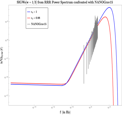
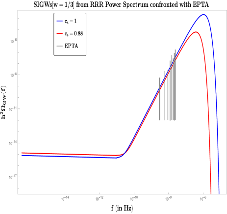
Figure 1: GW spectrum $h^{2}\Omega_{\rm GW}$ versus the frequency for different choices of the effective sound speed, $c_{s}=1$ (blue) and $c_{s}=0.88$ (red), while keeping the EoS $w=1/3$ fixed. The background consists of the experimental signal, shown here in black vertical lines, obtained by the NANOGrav15 (left) and EPTA (right) observations. The generated GW spectrum displays a growing trend consistent with the signals’ features, and soon after, it falls sharply due to the exponentially decreasing amplitude feature present inside the regularized-renormalized-resummed scalar power spectrum in Eqn. (21).

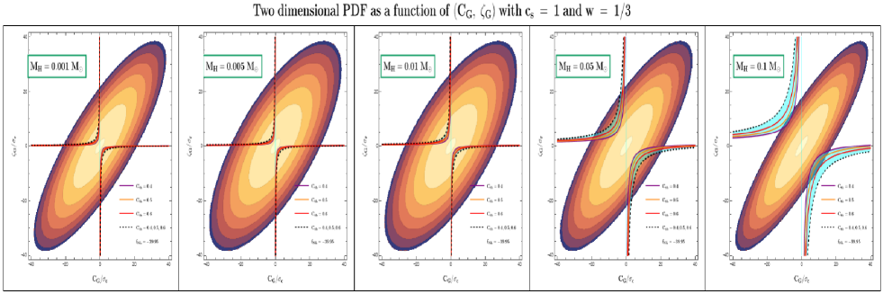
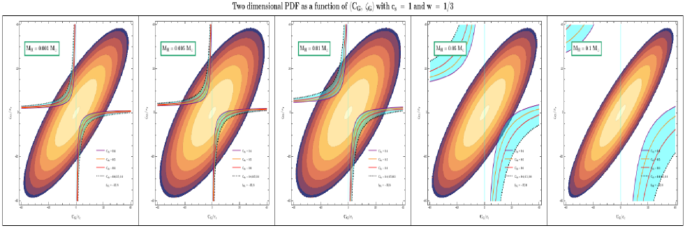
Figure 2: Joint probability distribution function for various values of PBH masses with a fixed amplitude $A=10^{-2}$, EoS parameter $w=1/3$, and effective sound speed $c_{s}=1$. The top fig. 2 depicts results for $f_{\rm NL}=-39.95$ while in the bottom fig. 2 corresponds to $f_{\rm NL}=-35/8$. The shaded cyan regions represent the permissible integration domains, from Eqn. (67), for various compaction thresholds: ${\cal C}_{\rm th}=0.4$ (purple), ${\cal C}_{\rm th}=0.5$ (yellow), ${\cal C}_{\rm th}=0.6$ (red), respectively. Inside the PDFs, we observe increased support of the domains giving over-threshold perturbations for lower mass PBH while these lose support by moving outwards for higher mass PBH. This effect becomes pronounced in the bottom for $f_{\rm NL}=-35/8$. As we increase the PBH mass, the correlation coefficient $\gamma_{\rm cr}$ tends towards unity, which is evident here by the compression along the correlated direction of the PDF.

VI.2 GW Spectrum

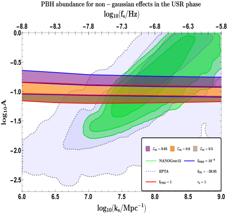
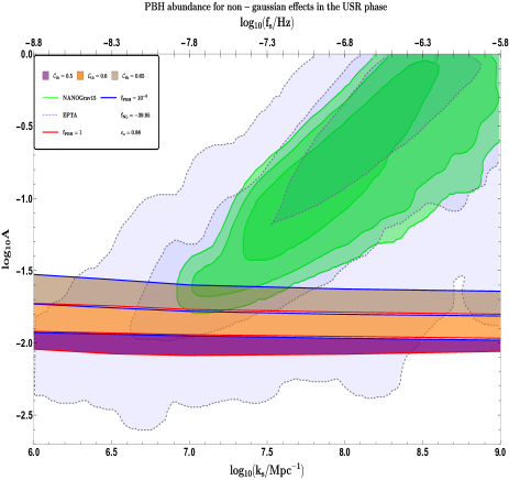
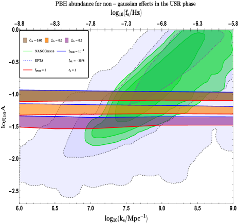
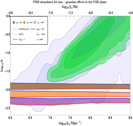
Figure 3: Variation in the USR peak amplitude $A$ of the regularized-renormalized-resummed power spectrum with the transition wavenumber $k_{s}$. The horizontal coloured bands highlight the region with abundance in the range $f_{\rm PBH}\in(10^{-3},1)$ relating to the distinct compaction thresholds, ${\cal C}_{\rm th}=0.65$ (light brown), ${\cal C}_{\rm th}=0.6$ (orange), ${\cal C}_{\rm th}=0.5$ (purple). The left plots of fig. 3 and fig. 3 utilize $c_{s}=1$, while the right plots of fig. 3 and fig. 3 have $c_{s}=0.88$. In the top row $f_{\rm NL}=-39.395$ is fixed while in the bottom row it is $f_{\rm NL}=-38/5$. Both large negative PNG, $f_{\rm NL}=-39.395$, with greater sound speed, $c_{s}=1$, introduce a much significant difference in the peak amplitude than any other combination of the two values. The light blue and the green posteriors correspond to EPTA and the NANOGrav15 data, respectively, and underlay the bands to enable the SIGW interpretation [23].

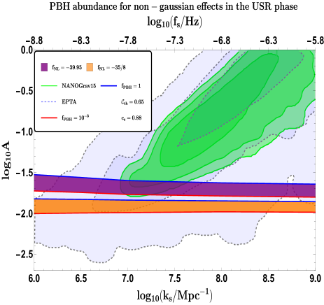
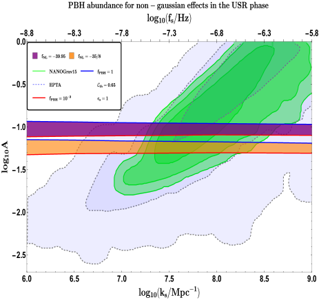
Figure 4: Plots demonstrating the impact of the effective sound speed parameter $c_{s}$ on the power spectrum amplitude $A$ in the USR phase. Both the figures contain comparisons between the two values of $f_{\rm NL}=(-39.95,-35/8)$ shown with blue and orange colours, respectively. In fig. 4, corresponding to $c_{s}=0.88$, the amplitude of both bands associated with two distinct $f_{\rm NL}$ parameters, is decisively excluded beyond the $1\sigma$ contours of the NANOGrav15 (green) and the EPTA (light blue) posteriors. In contrast, fig. 4, which employs $c_{s}=1$, provides a surge in the power spectra amplitude for both the bands and are well supported by the PTA data within the $1\sigma$ region.

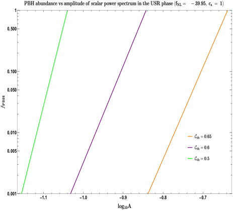
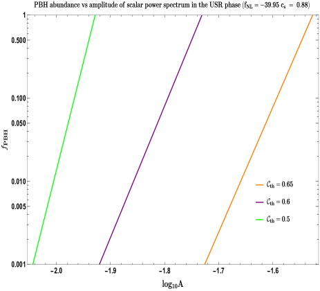
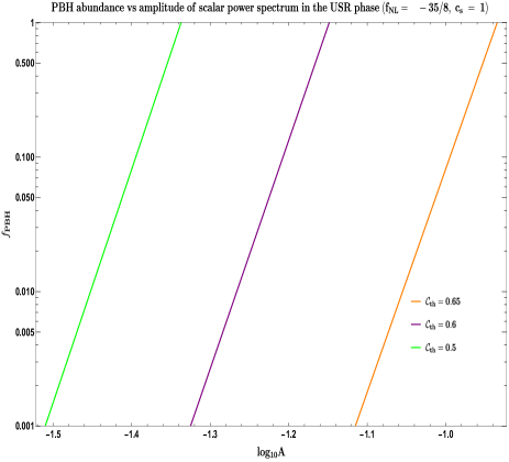
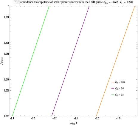
Figure 5: The PBH fractional abundance $f_{\rm PBH}$ plotted against the change in peak amplitude $A$ of the regularized-renormalized-resummed scalar power spectrum from the EFT of bounce. The top-left (5) and top-right (5) figures exploits $f_{\rm NL}=-39.395$, with the effective sound speed $c_{s}=1$ and $c_{s}=0.88$, respectively. The bottom-left (5) and bottom-right (5) figures exploits $f_{\rm NL}=-35/8$, with $c_{s}=1$ and $c_{s}=0.88$, respectively. In each sub-figure, the impact of changing threshold ${\cal C}_{\rm th}$ between ${\cal C}_{\rm th}=0.65$ (orange), ${\cal C}_{\rm th}=0.6$ (purple), and ${\cal C}_{\rm th}=0.5$ (green), on the $f_{\rm PBH}$ is illustrated along with the transition number kept fixed at the same value $k_{s}=10^{7}{\rm Mpc^{-1}}$. Notice the sudden fall in the observed fraction of PBHs as the amplitude gets slightly altered for a given threshold.

We employ our EFT of bounce setup to derive the behaviour of the fractional GW energy density as a function of the frequency, with the results shown in figure 1. In Fig. 1, the spectrum crosses the NANOGrav15 signal, and in Fig. 1, it crosses the EPTA signal. Both images illustrates that the generated spectrum covers the frequency bins probed by the PTA observations. Following this, the spectrum rapidly drops to zero due exponential damping effect inherent in the quantum-loop corrected power spectrum of Eqn. (21). In both the figures, we choose to highlight the difference coming from two different sound speed $(c_{s}=1,0.88)$ values which is motivated by the previous results on the total loop corrected power spectrum by the authors in [240]. After crossing the observed signals, the GW spectrum with $c_{s}=1$ exhibits larger amplitude by an order of magnitude relative to the spectrum with the choice of $c_{s}=0.88$. This analysis suggests that $c_{s}=1$ proves to be a more preferable choice to achieve a significant signal from SIGWs and its implication will also be reflected in our upcoming analysis of PBH formation.

VI.3 PBH Overproduction

In this study, we specifically focus our analysis on two principal values of the NG parameter, namely $f_{\rm NL}\in(-39.95,-35/8)$, justifications as to why have been detailed before in Sec. VI.3. Having established that, we begin our discussion with the figure (2), which depicts the 2D joint PDF with a uniform correlation between the variables ${\cal C}_{G}$ and ${\cal\zeta}_{G}$ for a spectrum of horizon masses in increasing order from left to right. The analysis has been carried out with EoS $w=1/3$, effective sound speed $c_{s}=1$, a fixed power spectrum amplitude $A=10^{-2}$ and two aforementioned values of the NG parameter, $f_{\rm NL}=-39.95$, and $f_{\rm NL}=-35/8$, as represented by figure 2 and figure 2 respectively. A noteworthy feature here is the non-uniqueness of the amplitude chosen. $A=10^{-2}$ denotes a baseline value beneath which the PBH abundance for all masses is significantly suppressed, rendering it unsuitable for meaningful analysis. This value is merely a critical minimum necessary to generate a substantial abundance of PBHs. Performing analysis with higher values of $A$ will also provide desirable results, provided the perturbation theory is kept intact. Furthermore, the amplitude value is chosen autonomously, without direct correspondence with the Gaussian variables ${\cal C}_{G}$, and $\zeta_{G}$. $A$ is anchored at $10^{-2}$ across all generated plots. Nevertheless, the PDF expression encapsulates $A$ through the different covariance elements. By modulating the Gaussian variables $({\cal C}_{G},\zeta_{G})$ for a particular $A$, we derive our PDF contour. The integration domains are permitted as per the Eqs. (67-71) (details of which have been provided in the Sec. IV.2.2), and delineated by the cyan bands in figure (2) with different separation boundaries corresponding to distinct thresholds of the compaction function, namely ${\cal C}_{\rm th}\in(0.4,0.5,0.6)$. These benchmark thresholds reside within the interval $[2/5,2/3]$, that is obtained after not fully considering the non-linear effects to the perturbation profile at super-horizon scales in the gradient-expansion approach [461].

Moving forward, it is crucial to emphasize that we follow the results of [461], where the entire analysis to determine the threshold ${\cal C}_{\rm th}$ has been performed with consideration of the NGs arising from the non-linear relationship between the density contrast and the curvature perturbation $\zeta$. However, PNGs have not been taken into account for calculating the threshold values. While several studies have examined the impact of PNGs on these threshold values [460, 465], no deviations, from the linear case result, with a significant impact of greater than an order of percent level have been recorded. Nonetheless, incorporating PNGs in estimating the threshold itself is beyond the scope of this paper’s current analysis.

With this consideration in mind, we return to the analysis of figure (2). Notably, all ${\cal C}_{\rm th}$ values share one common boundary denoted by the dotted black line. The iso-contours lines for $f_{\rm NL}=-39.95$ (figure 2) show a pronounced overlap of the domain with the PDF for lower masses, indicating a greater probability of obtaining sizeable abundance for these lower mass PBHs than for the higher mass. A parallel trend is evident for $f_{\rm NL}=-35/8$ (figure 2), where the domain gets drawn inwards for the low masses. However, a direct comparison between the two $f_{\rm NL}$ values reveals that contour lines for $f_{\rm NL}=-39.95$ exhibit a greater compatibility with the domain within the distribution. This implies that $f_{\rm NL}=-39.95$ is more favourable for the scenario of ample PBHs production as compared to $f_{\rm NL}=-35/8$. The above observation is further corroborated by the illustrations in the plots of figure (3), which demonstrates the influence of NGs on the power spectrum, varying along with the transition wavenumber $k_{s}$ in the USR region, necessary to obtain a suitable range of fractional abundance and subsequently avoid overproduction. The results are correlated with the PTA data to seek observational constraints. The various coloured bands represent the PBHs abundance in the range $f_{\rm PBH}\in(10^{-3}-1)$ corresponding to thresholds ${\cal C}_{\rm th}\in(0.5,0.6,0.65)$. Before diving into the discussion of the figure, we like to present a detail about the suitability of our forthcoming analysis with the NANOGrav15 and EPTA posteriors. A careful examination will display a resemblance of our chosen scalar power spectrum with the log-normal power spectrum. It is indebted to the presence of a USR phase with a sharp peak. This resemblance justifies our use of the PTA log-normal based posteriors for analysis. Additionally, the SIGW spectrum displayed in fig.(1) also exhibits a causality tail in the IR region, which is a distinctive feature when using the log-normal power spectrum. This further reinforces the idea that a separate probability analysis is not required in our case to develop the posteriors for deriving our outcomes.

Now, in figure 3 with $f_{\rm NL}=-39.95$, and $c_{s}=1$, we observe that all the bands corresponding to the threshold values yield substantial abundance with amplitudes in the range of $A\in(10^{-1}-10^{-0.5})$. Consequently, they effectively circumvent the overproduction problem by residing within the $1\sigma$ region of the NANOGrav15 posteriors. Conversely, reducing the magnitude of the negative $f_{\rm NL}$ to $-35/8$, and keeping $c_{s}=1$, would alter the results as shown in figure 3. Here for the threshold ${\cal C}_{\rm th}=0.65$ (brown band), both the upper and lower limits of the $f_{\rm PBH}$ fall within the $1\sigma$ region of the NANOGrav15 and EPTA contours, while for ${\cal C}_{\rm th}=0.6$ (orange band), the upper value of $f_{\rm PBH}$ merely grazes from outside of the $1\sigma$ contour of the EPTA. Additionally, for ${\cal C}_{\rm th}=0.5$ (purple band) in figure 3, the result is further constrained by being excluded at over the $1\sigma$ contour of the EPTA and barely grazes the $1\sigma$ region of the NANOGrav15. This observation aligns well with the theoretical expectations since the perturbation amplitude is intricately linked with the compaction threshold, and a higher ${\cal C}_{\rm th}$ within the linear regime necessitates a greater amplitude to generate the same fractional abundance as compared to lower values of the same. A similar trend is visible if we take $c_{s}=0.88$ and examine their results from the figs. (3, 3) for the two distinct $f_{\rm NL}$ cases. However, if we instead draw a direct comparison to inspect the impact of the effective sound speed $c_{s}$ on the amplitude, we can readily witness a significant difference separately captured in figure 4.

The left 4 and right 4 figures represent the variation of the power spectra amplitude with $k_{s}$ for $c_{s}=0.88$, and $c_{s}=1$, respectively. The plots have been realized with ${\cal C}_{\rm th}=0.65$. Figure 4 demonstrates both the bands, i.e. the orange for $f_{\rm NL}=-39.95$, and purple for $f_{\rm NL}=-35/8$ remain largely excluded over the $1\sigma$ region of the PTA contours. While the orange band circumvents overproduction and marginally favours the $2\sigma$ region of the NANOGrav15 contour, the scenario with $f_{\rm NL}=-35/8$ fails to generate sufficient amplitude to achieve comparable abundance while simultaneously remaining consistent with the NANOGrav15. Attempts to amplify the amplitude to conform to the SIGW interpretation of the NANOGrav15 data would bring the risk of overproducing PBHs. Now, in contrast, figure 4 temptingly highlights a dramatic surge in the amplitude for both the $f_{\rm NL}$ values. This remarkable shift prompted by the alteration of $c_{s}$ underscores the sensitivity of the setup to the effective sound speed parameter. Lowering $c_{s}$ from $1$ to $0.88$ drops the power spectrum amplitude to $A=10^{-3}$, an order of magnitude less when compared to $c_{s}=1$. This reduction in amplitude is consequential because it directly impacts the conditions requisite for PBH formation, as amplitude is integrated into the $f_{\rm PBH}$ through the Eqn. (72). The likelihood of PBH production drops further, drastically dropping for choices below $c_{s}=0.88$, making such scenarios irrelevant for analysis. Moreover, restraining to $c_{s}\leqslant 1$ is essential to uphold the causality constraints. Exceeding $c_{s}=1$ would jeopardize the perturbativity conditions and therefore can be ruled out.

Additionally, we notice the appearance of features in the width of the bands of figure (3). Notably, they are not uniform across the transition wavenumbers $k_{s}$. These bands are seen to exhibit greater thickness near $k_{s}\sim{\cal O}(10^{6}{\rm Mpc^{-1}})$ and become narrower towards the right side of the plots. Note that the transition wavenumber is linked with the PBHs mass by Eqn. (63). This is indicative of the idea that with increased wavenumber, PBHs with lower masses are poised to produce substantial abundance with a slightly lesser amplitude as compared to those with higher masses.

We now examine the results for the fractional abundance of PBHs represented by the figure (5). The three inclined coloured lines on each of these plots correspond to distinct compaction thresholds ${\cal C}_{\rm th}=0.65$ (orange), ${\cal C}_{\rm th}=0.6$ (purple), and ${\cal C}_{\rm th}=0.5$ (green). These lines depict the variation of the PBH abundance with the regularized-renormalized-resummed power spectrum amplitude for the two principal values of $f_{\rm NL}$ and $c_{s}$, recurrently mentioned in this paper. The transition wavenumber is kept fixed here at $k_{s}=10^{7}{\rm Mpc^{-1}}$. As clearly evident from the graphs, opting for a higher value of ${\cal C}_{\rm th}$ calls for a larger amplitude across all the generated plots, and vice versa. Further, to obtain a suitable $f_{\rm PBH}$ within the range $(10^{-3},1)$ with $(f_{\rm NL},c_{s})=(-39.95,1)$, we require a peak amplitude $A\sim{\cal O}(0.1)$. The abundance is extremely susceptible to the change in peak amplitude irrespective of the chosen threshold condition and any specific combination of the two $f_{\rm NL}$ and $c_{s}$ values. The scenario with $f_{\rm NL}=-35/8$ and $c_{s}=0.88$ (non-canonical) leads to the minimal amount of peak amplitude, while the negatively large $f_{\rm NL}=-39.95$ and $c_{s}=1$ (canonical) scenario leads to a huge amplification of $A$ which comes extremely close to breaching the perturbativity conditions. Now, having presented the results of our setup, let us look at how it compares to alternative frameworks and models previously studied to address the recent crucial overproduction problem.

VII Comparative analysis of previous studies

This section aims to address previous analyses conducted in line with studying the overproduction of PBHs and compares them through their efficiency and limitations in contrast to the approach adopted for this work and its results. Very recently, since the definitive announcement of an SGWB signal via the PTA collaborations, several groups have highlighted a dramatic issue concerning the abundant production of PBHs. This issue directly relates to having the SIGWs as a leading interpretation of the PTA signal. Upon its confrontation with the observed signal, it suggests a highly amplified scalar power spectrum, which implies that the PBHs can get overproduced. Below we discuss some of the major advances specific to this problem and supply the table1 summarizing the same.

Parameter	Ekpyrotic Bounce-USR	Matter Bounce-USR	Curvaton [23]	Galileon [237, 21, 18, 20]	MST [19, 22]
fNL	${\cal O}(-39.95)$	${\cal O}(-35/8)$	${\cal O}(-2)$	${\cal O}(-6)$	NYS
SIGW	Consistent with NANOGrav$15$ and EPTA	Consistent with NANOGrav$15$ and EPTA	Consistent with NANOGrav$15$ and EPTA	Consistent with NANOGrav$15$ and EPTA	Consistent with NANOGrav$15$ and EPTA
Over-production	Sharply within $1\sigma$ of NANOGrav$15$ and EPTA contours	Barely touches $1\sigma$ of EPTA contours	Within $2\sigma$ of NANOGrav$15$ and EPTA contours	Just enters inside the $1\sigma$ of NANOGrav$15$	Within $2\sigma$ of EPTA and just touches the $2\sigma$ of NANOGrav$15$
PBHs Mass ($M_{\odot}$)	$(10^{-6}-0.1)$	$(10^{-6}-0.1)$	$(10^{-6}-0.01)$	$(10^{-6}-0.1)$	$(10^{-31}-10^{4})$
EoS parameter	$(0.31,1/3)$	$(0.31,1/3)$	$1/3$	$(0.24,1/3)$	($-0.01,1/3$)
QCD effects	NSY	NSY	Studied	Studied	NSY
Quantum loop effects	$\bullet$ Consistent perturbative treatment   $\bullet$ Evades the no-go bound of $M_{\rm PBH}\sim{\cal O}(10^{2}{\rm gms})$	$\bullet$ Consistent perturbative treatment   $\bullet$ Evades the no-go bound of $M_{\rm PBH}\sim{\cal O}(10^{2}{\rm gms})$	NSY	$\bullet$ Consistent perturbative treatment   $\bullet$ Evades the no-go bound of $M_{\rm PBH}\sim{\cal O}(10^{2}{\rm gms})$	$\bullet$ Consistent perturbative treatment   $\bullet$ Evades the no-go bound of $M_{\rm PBH}\sim{\cal O}(10^{2}{\rm gms})$

Table 1: An overview on the results from studies on various models associated with the formation of curvature perturbations in the early universe. The models are compared based on various parameters that they have addressed. The abbreviation "NSY" indicates "Not Studied Yet" to denote parameters that have not been explored as of yet within a given model. Different PBH mass ranges investigated by the models have been expressed in the solar mass $M_{\odot}$ units. The values quoted for EoS parameter $w$ does not denote the best favourable outcomes of analysis, but rather the range of values utilized for investigation.

Among the many attempts to avoid this unfortunate outcome, some include the presence of an additional field that does not back-reacts to the dynamics of the background metric perturbations (a spectator field) like the curvaton model [307, 23, 308]. Much like the model discussed in this paper, the curvaton scenario in [67] also invites NGs into the PDF of $\zeta$ which is brought into effect by expansion of the curvature perturbation in terms of the leading order NG parameter $f_{\rm NL}$. In [67], using small and negative NGs, $f_{\rm NL}\sim{\cal O}(-1)$, the curvaton model is shown to provide a significant decrease in the abundance $f_{\rm PBH}$ thus avoiding overproduction while simultaneously explaining the SIGW from the PTA data. It is also able to generate large, solar mass, PBHs with $M_{\rm PBH}\sim{\cal}{O}(0.1-1)M_{\odot}$. Similarly, the analysis with curvaton in [307] shows that $f_{\rm NL}\sim{\cal O}(-1)$ generates the best possible outcomes for PBH formation while again conforming to the data from experiments (NANOGrav$15$ and EPTA). It was shown that by assuming a broken-power law power spectrum, and after using the similar quadratic curvature perturbation ansatz, the power spectrum peaked near $f_{\rm NL}=-2$ and on diving further below this value caused a substantial decrement in the amplitude required for PBHs formation. A similar effect has also been displayed considering positive $f_{\rm NL}$. Another notable example from these attempts involves using a spectator tensor field in [27], where the authors propose that it is this particular field responsible for the generation of the observed PTA signal and contributes sub-dominantly to the actual energy density fraction that is finally shared by the PBHs.

Using the equation of state parameter $(w)$, right before the RD era following inflation, is also shown as favorable by the authors in [19] to address the PBH overproduction issue when employed within the framework that contains multiple sharp transitions (MSTs) across a wide range of frequencies covering the PTA sensitivity and beyond. The authors here consider an EFT set-up with multiple SR-USR-SR phases in succession with a sufficient number of e-foldings $\Delta{\cal N}\sim(60-70)$ to complete inflation. This set-up is shown to generate a wide range of PBH masses ranging from sub-solar to beyond solar mass. Moreover, the SIGW spectrum generated from the one-loop corrected power spectrum also conforms to the NANOGrav15 data and other experimental data from LISA [481], DECIGO [482], Cosmic explorer (CE) [483], HLVK (LIGO, VIRGO, and KAGRA) [484, 485, 486], Einstein telescope (ET) [487], BBO [488]. In [19], after integrating the effect of varying $w$ within the MST set-up, a major conclusion drawn was to demonstrate that $w=1/3$ produces the best possible results to derive all the aforementioned outcomes. However, the mentioned studies do not include the effect of consideration of either non-linearity between the density contrast and the curvature perturbation or the PNGs, which is yet to be studied. Numerous studies have focused on employing local PNGs, and it is this particular feature of the curvature perturbations that has been the most effective in doing away with PBH overproduction. Previously, in section VI.1, we elaborated on the impact of having this feature within a theory to study PBH production, and many of the latest studies in [23, 285, 280, 118, 121, 71, 284, 20] illustrate this viewpoint thoroughly to examine the overproduction of PBHs. For the case of Galileon inflation, inferring from the results of [18], we observe that, with $f_{\rm NL}\sim{\cal O}(-6)$, it is able to cure the overproduction and strengthen the support for a SIGW explanation of the signal.

The emergence of QCD effects in the PTA signal stems from the sudden decrease in the energy and entropy degrees of freedom around the temperature, $T\gtrsim 100{\rm MeV}$, that aligns perfectly well within the regime of frequency probed by the PTA and thus the corresponding decrease in the equation of state can noticeably alter the low-frequency tail of the signal [489]. Using such conditions for Galileon inflation, [20] shows the softening of the IR tail of the GW spectrum till $f\simeq 5\times 10^{-9}{\rm Hz}$, that is, before we reach the peak of the spectrum. In the present study however, QCD effects have not been taken into account for formation of PBHs.

In the last row, we consider the case where quantum loop effects are considered while estimating the results on PBH production from a model of interest. In the light of the no-go theorem [233, 234, 235], all the studies mentioned, except for the curvaton, come as examples of how to successfully evade the stringent bound, $M_{\rm PBH}\sim{\cal O}(10^{2}{\rm gms})$, as a consequence of this theorem.

The present work applies the same spirit of using the PNGs to our advantage but goes a step further by taking into account enormous values for the same, $f_{\rm NL}\ll{\cal O}(-10)$, in comparison to the previous studies. This work also exploits the compaction function approach rather than the standard Press-Schechter formalism or the method from peaks theory to study the PBH formation process. And at last, the underlying set-up of this paper goes beyond the choice of working just within the inflationary picture, that numerous other studies above prefer to address this issue, but also combines the features and consequences of having a non-singular bouncing scenario before the usual slow-roll commences. To conduct the analysis for the overproduction problem, with section VI.3 devoted towards its end results, we utilize the theoretical set-up that is built upon the works [233, 234, 235, 240] and by integrating the aforementioned improvements we aim to achieve a stronger and broader understanding on curing the overproduction along with shedding some light in an upcoming section on the acceptable amounts of such type of NGs.

VIII Confrontation with experiments

After conducting an elaborate discussion including various models and their relationship with multiple parameters encountered during PBH formation, we briefly discuss in this section their results when confronted with different gravitational wave experiments and, if possible, microlensing experiments for searching signatures of dark matter. The summary of these results can be observed through table 2.

Experiment	Ekpyrotic Bounce-USR	Matter Bounce-USR	Galileon [18, 19]	Curvaton [307, 308, 23]	MST [22]
EPTA	Consistent SIGW signal generation	Consistent SIGW signal generation	Consistent SIGW signal generation	Consistent SIGW signal generation	Consistent SIGW signal generation
NANOGrav15	Consistent SIGW signal generation	Consistent SIGW signal generation	Consistent SIGW signal generation	Consistent SIGW signal generation	Consistent SIGW signal generation
LVK	NSY	NSY	Similar strength of $\Omega_{\rm GW}h^{2}$ inside the LVK constraints as for the PTA	NSY	Uniform strength of $\Omega_{\rm GW}h^{2}$ across all transitions into the LVK
Microlensing	Possible to generate $\log_{10}{(M_{\rm PBH})}\sim{\cal O}(-6,-2)$ with $f_{\rm PBH}\in(10^{-3}-1)$ and consistent with the PTA	Similar result to the Ekpyrotic section	Maximum possible value $f_{\rm PBH}\sim 10^{-1.6}$ for $M_{\rm PBH}\sim 10^{-2}M_{\odot}$ and $w=1/3$ after constraints from EROS/MACHO	Generates asteroid mass PBHs with $f_{\rm PBH}\lesssim 1$, after constraints from SUBARU HSC.	Maximum possible value $f_{\rm PBH}\sim 10^{-1.7}$ for $M_{\rm PBH}\sim{\cal O}(10^{-4}M_{\odot}$) and $w=1/3$ after constraints from OGLE

Table 2: Various experiments and their conclusions have been highlighted in the light of PBH formation, and SIGW interpretation. "NSY" denotes that the parameter is "Not Studied Yet" inside that specific model.

Among the list of experiments, we focus here on the PTA (NANOGrav and EPTA) observations that cover the nanohertz (nHz) and beyond frequency range of $f\sim{\cal O}(10^{-9}-10^{-7}){\rm Hz}$ and corresponds roughly to probing PBHs with masses, $M_{\rm PBH}\sim{\cal O}(10^{-4}-10^{-2})M_{\odot}$. Then there are the microlensing experiments, namely the Subaru HSC [490], OGLE [491], EROS/MACHO [492], that can provide tight constraints covering the PBH mass range, $M_{\rm PBH}\sim{\cal O}(10^{-10}-10^{-1})M_{\odot}$. And following this, at frequencies $f\sim{\cal O}(1-10^{3}){\rm Hz}$, we have constraints coming from the LIGO, VIRGO, and KAGRA (LVK) gravitational wave observatories that can probe PBH masses with $M_{\rm PBH}\sim{\cal O}(0.1)M_{\odot}$. We then collect results on PBH formation from various models as listed along the top row of the table 2 and comment on them if any study utilizing that model concerns the regime probed by the above experiments.

Beginning with the model focused on in the present work, our EFT treatment helps us to combine the contraction and bouncing scenarios, regardless of their kind, either ekpyrotic or matter, with the inflationary framework that contains a USR phase for PBH generation. In the figure (1), we show that under the choice of $w=1/3$ for the RD era, and either choice of $c_{s}$, the resulting SIGW spectrum follows consistently both the PTA (NANOGrav$15$ and EPTA) signals in their respective frequency regimes. This conclusion does not alter whether choosing the ekpyrotic case $(\epsilon_{c/b}>3)$ or the matter case $(\epsilon_{c/b}=3/2)$ before inflation, thereby giving us a positive signature upon confrontation with the PTA experiments. A dedicated analysis focusing on the high-frequency LVK regimes is yet to be performed for this model. For the case of Galileon inflation, the analysis in [21] suggests the conclusive feature of the resulting SIGW spectrum with the PTA signals. Due to the benefits coming from the non-renormalization theorem, as elaborated in [236, 21], the spectrum can provide enough signature inside the frequency regime probed by the LVK observations while preserving its similar features as in the low-frequency PTA regime. While in [308], asteroid mass PBHs with $M_{\rm PBH}\sim{\cal O}({10^{-16}-10^{-10}})M_{\odot}$, probed by SUBARU HSC [490], and produced in the curvaton models can explain the totality of dark matter depending on the duration of the curvaton decay, the curvaton mass and Hubble scale at the end of inflation. In the case of having multiple sharp transitions [22], the SIGW spectrum, once generated, has the feature, owning to the setup, to provide for a signature consistent with both the observed nHz regime of the PTA signal and the high-frequency regime probed by the LVK.

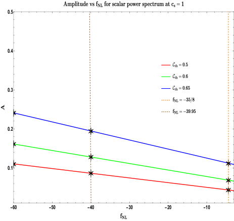
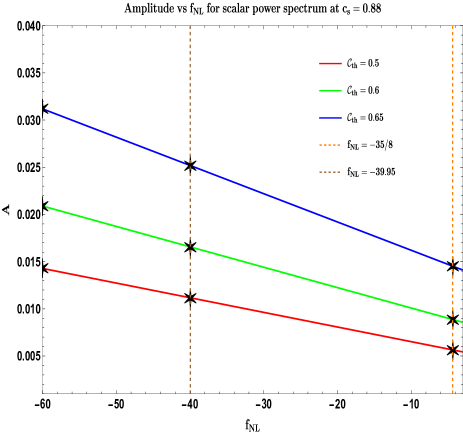
Figure 6: Plots highlighting the variation of peak amplitude $A$ of the power spectrum with the non-Gaussianity parameter $f_{\rm NL}$ for separate cases of the effective sound speed $c_{s}$. The left figure (6) corresponds to $c_{s}=1$, where the amplitude achieves a noticeable amplification, standing around an order of magnitude higher than the right figure (6) which employs $c_{s}=0.88$. Both figures incorporate distinct compaction thresholds, specifically ${\cal C}_{\rm th}\in(0.5,0.6,0.65)$, denoted by red, green, and blue lines respectively. The red and green dotted vertical lines mark the position of the values $f_{\rm NL}=(-39.95,-35/8)$ that we incorporate continuously within our analysis, and these intersect with the various coloured inclined lines for separate values of $A$ marked using a solid star. We establish an upper bound on the value of $f_{\rm NL}$ through this observation.

IX Establishment of strong upper bound on $f_{\rm NL}$

This work has delved into the significance of having large and negative primordial non-Gaussianity in our theory to evade the issue of PBH overproduction. In section VI.3, we show through our results how large NGs, with value $f_{\rm NL}\sim{\cal O}(-40)$, can not only suppress the overproduction of near-solar mass PBHs but the corresponding curvature perturbations can lead to an induced GW spectrum that successfully aligns with the latest PTA observations. We now recall the discussions in Sec. VI.1 about having such large magnitude of NGs within our theory as a direct signature of violating the famous consistency condition for single-field, slow-roll inflation proposed by Maldacena in [300] which suggests $f_{\rm NL}\sim{\cal O}(-0.1)$. Instead, if one assumes a contracting phase followed by a matter bounce scenario, then, as pointed out in [301], the strength of NGs increases due to their amplitude getting unaffected by the slow-roll parameters, and the curvature perturbations in the contracting phase constantly experience growth in the super-horizon scales until the matter bounce initiates. The other interesting aspect is the scenario of an ekpyrotic contraction before the bouncing phase. During this phase, the potential well becomes negative, extremely steep, and increases the kinetic energy density in the scalar fields to dominate, leading to highly non-linear interactions and thus resulting in an increase in the non-Gaussian signature from such a phase. The corresponding ekpyrotic equation of state controls the largeness of the interactions. We work with the results in [302], where they discuss the production of NGs in the ekpyrotic(and cyclic) models in great detail. During the contraction phase, the scalar field fluctuations produce the entropic perturbations, which later get converted into the curvature perturbations where the EoS in this intervening instant of conversion, right before going into the bounce, significantly affects the non-Gaussianities. If such a conversion occurs during the ekpyrotic phase, it can produce a favorable amount of negative and large NGs of order $f_{\rm NL}\ll{\cal O}(-10)$.

In our results, it is evident from figures (3-5) that the requisite peak scalar power spectrum amplitude is quite substantial, $A\sim{\cal O}(0.1)$, which approaches to the verge of breaking the underlying perturbative approximation. At this point, we ask ourselves, how large can we expect the magnitude of NG to grow before it breaches this approximation? To address this, we examine the figure (6).

The need for amplified strength of inflationary fluctuations for PBH formation does not necessarily warrant the validation of perturbativity constraints. From the figure (6), we observe a monotonic trend for the peak amplitude $A$ with increasing magnitude of the NG parameter $f_{\rm NL}$. Our previous results have shown how helpful large negative NGs are in dealing with PBH overproduction. Presently, in both figures 6 and 6, we can see that the amplitude $A$ required to achieve $f_{\rm PBH}\sim 1$, increases with negative $f_{\rm NL}$ as well as with higher values of the compaction threshold ${\cal C}_{\rm th}$. However, there comes a moment where the required amplitude crosses over $A\sim{\cal O}(0.1)$ for both $f_{\rm NL}=(-39.95,-35/8)$ and $c_{s}=1$ and over $A\sim{\cal O}(0.01)$ for the same set of $f_{\rm NL}$ but now with $c_{s}=0.88$. Following our repeated emphasis over choosing the canonical case where $c_{s}=1$, we notice from figure 6 that going beyond $f_{\rm NL}\sim-60$ will surely keep pushing the amplitude close of eventually hit $A\sim{\cal O}(1)$ and putting the analysis at risk of breaking perturbativity. In a similar spirit, with $c_{s}=0.88$ in figure 6, one observes the condition $A>0.01$ for $f_{\rm NL}\lesssim-60$. Furthermore, since we aim for the interval, $f_{\rm PBH}\in(10^{-3},1)$, that quantifies as having a sizeable fraction, the maximum amplitude difference tolerable for a particular wavenumber comes to be, $\log_{10}(\Delta A)=-0.2$, which is an estimate that we can expect even when we consider $f_{\rm NL}\sim{\cal O}(-60)$.

For the space of allowed compaction thresholds, the values that we have considered here for ${\cal C}_{\rm th}$ lie in between $(0.5,0.65)$, with ${\cal C}_{\rm th}=0.5$ demanding the amplitude to come just close to $A\sim 0.1$. And so, any value of this threshold lower than ${\cal C}_{\rm th}\sim 0.5$ will accordingly require a low enough amplitude even if we consider $f_{\rm NL}\sim-60$. Thus, we conclude that for $0.4<{\cal C}_{\rm th}<0.5$, where the lower limit arises from our choice of working with the linear regime result, ${\cal C}_{\rm th}\in[2/5,2/6]$ [461], the strength of the scalar power spectrum is still sufficient to incorporate further large and negative NG, $f_{\rm NL}<-60$. The significance of $f_{\rm NL}=-60$ also extends to the fact that in the figure (6) we choose to show the analysis for the same set of compaction thresholds that we previously incorporate in figures (3-5) to highlight the removal of PBH overproduction with the choice of ${\cal C}_{\rm th}\in(0.5,0.65)$ giving us the best agreement with the data.

Considering the pre-inflationary dynamics of the perturbations, studies have pointed out that, in principle, one great advantage of such conditions is the generation of a large amount of NG that reaches upto $f_{\rm NL}\sim{\cal O}(100)$ [302, 480]. In such cases, we can, however, comment about large NGs as our use of an EFT framework encompasses both the scenarios before the beginning of inflation and hereafter, thus allowing for a generalized study. Hence, concluding from the observations, we provide a stringent upper bound on the possible magnitude of NG, $f_{\rm NL}\sim-60$, that does not endanger the validity of our analysis within our EFT setup.

X Conclusion

In this section, we summarize our crucial findings regarding the cure for PBH overproduction and its connection with exhibiting large and negative primordial non-Gaussianities. Our underlying set-up takes advantage of the features coming from pre-inflationary physics, with the introduction of the contracting and bouncing phases, into the generation of extremely large non-Gaussianities in the curvature perturbations. The benefit of bearing such large NGs is reflected in controlling the abundance of PBHs, which are formed during inflation, and they determine whether their abundance gets either suppressed or enhanced. We began with a brief introduction on the EFT of bounce framework built on the works of [233, 234, 235, 240], and described how the scalar power spectrum after contributions from each phase gets constructed including the one-loop quantum corrections. In order to provide a lucid procedure of handling the quantum-loop corrections, we summarize its main components of regularization, renormalization, and resummation which altogether assist in removing any quadratic (or power-law) UV and smoothen the logarithmic IR divergences resulting from each phase to the tree level result. At the end of the procedures, we obtained the crucial one-loop renormalized and DRG resummed scalar power spectrum through which we later discuss the production of PBHs.

Keeping in line with the latest surge in the theoretical advancements of PBH formation, we preferred to employ the compaction function criterion for the same and elaborate on its formalism which provides a means to calculate the PBH mass fraction. We further integrate the inclusion of quadratic form of NGs within the compaction function approach, to conduct a qualitative study of the impact NGs have on PBH formation. We follow this with a discussion on how we go about calculating the necessary abundance and the effect of having PNGs in such calculations. After this, we take a brief interlude to discuss the energy density spectrum of the scalar induced gravity waves in the radiation dominated era where $w=1/3$. Throughout this work, we do not entertain any free equation of state and proceed with the fact that the scales contributing most to the PBH collapse do so after their re-entry into the radiation era, for a general equation of state analysis within the EFT of bounce set-up we refer to [303].

In the latter half of this paper, we focused primarily on the outcomes after getting the help of large and negative PNGs to tackle the overproduction of PBHs. To better comprehend the crucial insights gained from the rest of our analysis, we illustrate them using bullet points as follows:

• We selected two distinct benchmark values for investigating PNGs namely, $f_{\rm NL}=(-39.95,-35/8)$, which result from independent analysis focusing on either an ekpyrotic contraction [302] or an expanding period of matter bounce [301], respectively. Within this analysis, we added another variable - effective sound speed component and considered its two separate values, $c_{s}=(0.88,1)$ based on a previous work [240].

• We found from our set-up that the probability of producing near solar mass PBHs, $M_{\rm PBH}\geqslant{\cal O}(0.01)M_{\odot}$, kept decreasing at a faster rate when $f_{\rm NL}=-35/8$ than in the case where $f_{\rm NL}=-39.95$, signalling the importance of large and negative PNGs in the PBH production probability for a given amplitude of the scalar power spectrum.

• To highlight our best result, we established that larger negative values like $f_{\rm NL}=-39.95$, coupled with the canonical case $c_{s}=1$, proved utmost beneficial in increasing the abundance of PBHs and simultaneously establishing an excellent agreement of the requisite peak power spectrum amplitude within $1\sigma$ of having a SIGW explanation of the recent PTA signal.

• Utilizing a lower value of $c_{s}=0.88$ lead to an order of magnitude suppression in the amplitude, pushing the agreement to outside the $2\sigma$ regime when $f_{\rm NL}=-39.95$ and even outside by $3\sigma$ for the choice of $f_{\rm NL}=-38/5$.

• After this, we conducted a comparative study highlighting the latest attempts towards addressing overproduction through various models that either include just the PNGs to their advantage or incorporate other new parameters. We followed this by confronting these models’ results with a few observational experiments for detecting gravitational wave signals and candidates for dark matter via microlensing.

• Later, we scrutinized the acceptance of negatively large NGs in our EFT model and concluded this discussion by extracting an upper bound of $f_{\rm NL}\sim-60$ as the most allowable negative value for the case of large compaction thresholds, ${\cal C}_{\rm th}\in(0.5,0.65)$, utilizing which we earlier mitigated strongly the overproduction of PBHs.

• When going more negative beyond $f_{\rm NL}\sim-60$, we found the power spectrum amplitude to cross over the condition $A\sim{\cal O}(0.1)$ for $f_{\rm NL}=-39.95$, and also over $A\sim{\cal O}(0.01)$ for $f_{\rm NL}=-35/8$, which signalled a breach in the underlying perturbativity arguments.

Appendix

Appendix A Comoving curvature perturbation mode solutions

In this section, we underline the explicit curvature perturbation mode solutions for each phase in our EFT of bounce set-up. These solutions will later help us to construct the tree-level scalar power spectrum and are needed further to evaluate the various momentum and temporal integrals for the quantum loop corrections. The discussions related to one-loop quantum corrections are part of the next section. The upcoming results are basically solutions of the Fourier space MS equation, see Eqn. (9), for any wavenumber $k$. Our complete setup consists of $5$ phases, starting with the contraction, followed by a bounce into an expanding phase, which joins with the SRI as inflation begins, a sharp transition into the USR, and a sharp transition into the final SRII phase where inflation ends. For both contracting and bouncing phases, we do not restrict to any particular matter or ekpyrotic kind but generalize the study to suit either.

We begin below from the contracting phase and mention the mode solutions until the SRII phase and illuminate along the way the properties of each general solution.

1. Phase-I  (Contraction): The contraction phase of our set-up is characterized using the scale factor solution present in Eqn. (2) which involves the use of its equation of state parameter $\epsilon_{c}$ and determines whether its a matter $(\epsilon_{c}=3/2)$ or an ekpyrotic $(\epsilon_{c}>3)$ kind of phase. This phase operates during the conformal time interval, $\tau_{c}<\tau<\tau_{b}$, at the end of which we transition into the next bouncing phase. The curvature mode solution during contraction has the following structure:

   $${\bf\zeta}_{\bf C} = \frac{2^{\nu-\frac{3}{2}}c_{s}(-kc_{s}\tau)^{\frac{3}{2}-\nu}}{ia_{0}\tau\sqrt{2\epsilon_{*}}(kc_{s})^{\frac{3}{2}}\sqrt{2}M_{pl}}\left(\frac{\tau}{\tau_{0}}\right)^{-\frac{1}{(\epsilon-1)}}\sqrt{\left(\frac{\epsilon_{*}}{\epsilon_{c}}\right)}\Bigg{|}\frac{\Gamma(\nu)}{\Gamma(\frac{3}{2})}\Bigg{|}$$ (80)

   $$\quad\quad\quad\quad\quad\quad\quad\quad\quad\quad\quad\quad\times\Bigg{\{}\alpha_{1}(1+ikc_{s}\tau)e^{-i\left(kc_{s}\tau+\frac{\pi}{2}\left(\nu+\frac{1}{2}\right)\right)}-\beta_{1}(1-ikc_{s}\tau)e^{i\left(kc_{s}\tau+\frac{\pi}{2}\left(\nu+\frac{1}{2}\right)\right)}\Bigg{\}},$$

   where variable $\nu$ denotes the effective mass parameter from Eqn. (II). The above solution consists of a linear combination which comes with two Bogoliubov coefficients namely $\alpha_{1}$ and $\beta_{1}$ which provide information about the underlying quantum vacuum state and must satisfy the normalized condition $|\alpha_{1}|^{2}-|\beta_{1}|^{2}=1$. We must note here that in this work the choice of the initial vacuum structure is set to that of the Bunch-Davies vacuum which determines the coefficients with $\alpha_{1}=1,\;\beta_{1}=0$.

2. Phase-II  (Bounce): The expanding bounce phase is the second phase of our set-up which begins at $\tau_{b}$ and operates within the conformal time interval, $\tau_{b}<\tau<\tau_{i}$. This phase is characterized by its corresponding scale factor in Eqn. (3) and which also includes the equation of state parameter $\epsilon_{b}$ through which we are able to capture the matter $(\epsilon_{c}=3/2)$ or ekpyrotic $(\epsilon_{c}>3)$ bouncing scenario. The curvature mode solution during the bounce takes the following form:

   $${\bf\zeta}_{\bf B}=\frac{2^{\nu-\frac{3}{2}}c_{s}(-kc_{s}\tau)^{\frac{3}{2}-\nu}}{ia_{0}\tau\sqrt{2\epsilon_{*}}(kc_{s})^{\frac{3}{2}}\sqrt{2}M_{pl}}\left[1+\left(\frac{\tau}{\tau_{0}}\right)^{2}\right]^{-\frac{1}{2(\epsilon-1)}}\sqrt{\left(\frac{\epsilon_{*}}{\epsilon_{b}}\right)}\Bigg{|}\frac{\Gamma(\nu)}{\Gamma(\frac{3}{2})}\Bigg{|}$$

   $$\quad\quad\quad\quad\quad\quad\quad\quad\quad\quad\quad\quad\quad\quad\times\Bigg{\{}\alpha_{1}(1+ikc_{s}\tau)e^{-i\left(kc_{s}\tau+\frac{\pi}{2}\left(\nu+\frac{1}{2}\right)\right)}-\beta_{1}(1-ikc_{s}\tau)e^{i\left(kc_{s}\tau+\frac{\pi}{2}\left(\nu+\frac{1}{2}\right)\right)}\Bigg{\}}.$$ (81)

   Throughout this phase, the choice of underlying quantum vacuum remains the same as our initial Bunch-Davies scenario at the beginning of the contraction. We choose this kind of smooth transitory behaviour between these phases, till we enter inside the inflationary epoch, for the sake of ease in our calculations. The Bogoliubov coefficients therefore follow with $\alpha_{1}=1,\;\beta_{1}=0$, still keeping the normalization condition intact.

3. Phase-III  (First Slow-Roll): After the bouncing phase ends, we enter into inflation starting with the usual SR phase which lasts for the interval, $\tau_{i}<\tau<\tau_{s}$. Here the crucial assumption is that of the similar vacuum structure as before for the contraction and bounce phases. The general mode solution for this phase has the following form:

   $${\bf\zeta}_{\bf SRI} = \frac{2^{\nu-\frac{3}{2}}c_{s}H(-kc_{s}\tau)^{\frac{3}{2}-\nu}}{i\sqrt{2\epsilon_{*}}(kc_{s})^{\frac{3}{2}}\sqrt{2}M_{pl}}\Bigg{|}\frac{\Gamma(\nu)}{\Gamma(\frac{3}{2})}\Bigg{|}\Bigg{\{}\alpha_{1}(1+ikc_{s}\tau)e^{-i\left(kc_{s}\tau+\frac{\pi}{2}\left(\nu+\frac{1}{2}\right)\right)}-\beta_{1}(1-ikc_{s}\tau)e^{i\left(kc_{s}\tau+\frac{\pi}{2}\left(\nu+\frac{1}{2}\right)\right)}\Bigg{\}}.$$ (82)

   where the Bogoliubov coefficients remain the same as stated, $\alpha_{1}=1,\;\beta_{1}=0$. During the previous phases we did not assume any special kind of transitory behaviour when connecting the phases, but this changes soon as the SRI phases comes to an end at $\tau=\tau_{s}$.

4. Phase-IV  (Ultra Slow-Roll): The USR phase continues for the conformal time interval, $\tau_{s}<\tau<\tau_{e}$, where the assumption is that, at the beginning, the transition happens sharply without any relaxation. As a result of this transition nature, the underlying vacuum also undergoes a shift in its properties from the usual Bunch-Davies. The curvature mode solution now takes the following form:

   $${\bf\zeta}_{\bf USR} = \frac{2^{\nu-\frac{3}{2}}c_{s}H(-kc_{s}\tau)^{\frac{3}{2}-\nu}}{i\sqrt{2\epsilon_{*}}(kc_{s})^{\frac{3}{2}}\sqrt{2}M_{pl}}\bigg{(}\frac{\tau_{s}}{\tau}\bigg{)}^{3}\Bigg{|}\frac{\Gamma(\nu)}{\Gamma(\frac{3}{2})}\Bigg{|}\Bigg{\{}\alpha_{2}(1+ikc_{s}\tau)e^{-i\left(kc_{s}\tau+\frac{\pi}{2}\left(\nu+\frac{1}{2}\right)\right)}$$ (83)

   $$\quad\quad\quad\quad\quad\quad\quad\quad\quad\quad\quad\quad\quad\quad\quad\quad\quad\quad\quad\quad\quad\quad\quad\quad\quad-\beta_{2}(1-ikc_{s}\tau)e^{i\left(kc_{s}\tau+\frac{\pi}{2}\left(\nu+\frac{1}{2}\right)\right)}\Bigg{\}}.$$

   where we notice the appearance of two new sets of Bogoliubov coefficients namely, $\alpha_{2},\;\beta_{2}$. These coefficients can be calculated keeping in mind the above two formulas in Eqn. (82-83) and applying the continuity and differentiability conditions for the modes at the instant $\tau=\tau_{s}$ of the transition. Solving these boundary conditions would yield the following solutions for the coefficients:

   $$\alpha_{{2}} = \frac{1}{2k^{3}\tau_{s}^{3}c_{s}^{3}}\Bigg{(}3i+3ik^{2}c_{s}^{2}\tau_{s}^{2}+2k^{3}c_{s}^{3}\tau_{s}^{3}\Bigg{)},$$ (84)

   $$\beta_{{2}} = \frac{1}{2k^{3}c_{s}^{3}\tau_{s}^{3}}\Bigg{(}3i-6kc_{s}\tau_{s}-3ik^{2}c_{s}^{2}\tau_{s}^{2}\Bigg{)}e^{-i\left(\pi\left(\nu+\frac{1}{2}\right)+2kc_{s}\tau_{s}\right)},$$ (85)

   which describe the general solution in terms of the new shifted vacuum structure. Following this phase for a brief interval of time, we finally move to the last slow-roll phase at $\tau=\tau_{e}$.

5. Phase-V  (Second Slow-Roll): The USR phase further observes a sharp transition when passing over to the SRII phase and that operates within, $\tau_{e}<\tau<\tau_{0}$, after which inflation officially terminates. The vacuum, as a consequence of another sharp transition, witnesses further changes in its structure and a new set of Bogoliubov coefficients, $\alpha_{3},\;\beta_{3}$, are needed to describe the following general mode solution in this phase:

   $${\bf\zeta}_{\bf SRII} = \frac{2^{\nu-\frac{3}{2}}c_{s}H(-kc_{s}\tau)^{\frac{3}{2}-\nu}}{i\sqrt{2\epsilon_{*}}(kc_{s})^{\frac{3}{2}}\sqrt{2}M_{p}}\left(\frac{\tau_{s}}{\tau_{e}}\right)^{3}\Bigg{|}\frac{\Gamma(\nu)}{\Gamma(\frac{3}{2})}\Bigg{|}\Bigg{\{}\alpha_{3}(1+ikc_{s}\tau)e^{-i\left(kc_{s}\tau+\frac{\pi}{2}(\nu+\frac{1}{2})\right)}$$ (86)

   $$\quad\quad\quad\quad\quad\quad\quad\quad\quad\quad\quad\quad\quad\quad\quad\quad\quad\quad\quad\quad\quad\quad\quad\quad\quad-\beta_{3}(1-ikc_{s}\tau)e^{i\left(kc_{s}\tau+\frac{\pi}{2}(\nu+\frac{1}{2})\right)}\Bigg{\}}.$$

   where, via the similar continuity and differentiabilty condition applied to the solution in Eqn. (83-86), provides with the following new set of coefficients:

   $$\alpha_{3} = \frac{1}{(2k^{3}\tau_{e}^{3}c_{s}^{3})(2k^{3}\tau_{s}^{3}c_{s}^{3})}\Bigg{\{}\left(-3i-3ik^{2}\tau_{e}^{2}c_{s}^{2}+2k^{3}\tau_{e}^{3}c_{s}^{3}\right)\times\left(3i+3ik^{2}c_{s}^{2}\tau_{s}^{2}+2k^{3}c_{s}^{3}\tau_{s}^{3}\right)$$ (87)

   $$\quad\quad\quad\quad-\left(-3i-6k\tau_{e}c_{s}+3ik^{2}\tau_{e}^{2}c_{s}^{2}\right)\times\left(3i-6kc_{s}\tau_{s}-3ik^{2}c_{s}^{2}\tau_{s}^{2}\right)e^{2ikc_{s}(\tau_{e}-\tau_{s})}\Bigg{\}},$$

   $$\beta_{3} = \frac{1}{(2k^{3}\tau_{e}^{3}c_{s}^{3})(2k^{3}c_{s}^{3}\tau_{s}^{3})}\Bigg{\{}\left(-3i+6k\tau_{e}c_{s}+3ik^{2}\tau_{e}^{2}c_{s}^{2}\right)\times\left(3i+3ik^{2}c_{s}^{2}\tau_{s}^{2}+2k^{3}c_{s}^{3}\tau_{s}^{3}\right)e^{-\left(2ik\tau_{e}c_{s}+i\pi\left(\nu+\frac{1}{2}\right)\right)}$$ (88)

   $$\quad\quad\quad\quad+\left(2k^{3}\tau_{e}^{3}c_{s}^{3}+3ik^{2}\tau_{e}^{2}c_{s}^{2}+3i\right)\times\left(3i-6kc_{s}\tau_{s}-3ik^{2}c_{s}^{2}\tau_{s}^{2}\right)e^{-i\left(\pi(\nu+\frac{1}{2})+2kc_{s}\tau_{s}\right)}\Bigg{\}}.$$

Appendix B One-loop corrections using In-In formalism

In this appendix we describe the approach towards calculating the one-loop quantum corrections to the $2$-point correlation function using the well-known in-in formalism in cosmology.

For this aim, we require the cubic order expansion [300] of the EFT action for the curvature perturbation whose final form reads as:

$$S^{(3)}_{\zeta}=\int d\tau\;{\cal L}_{3}=\int d\tau\;d^{3}x\;M^{2}_{pl}a^{2}\;\bigg{[}\left(3\left(c^{2}_{s}-1\right)\epsilon+\epsilon^{2}-\frac{1}{2}\epsilon^{3}\right)\zeta^{{}^{\prime}2}\zeta+\frac{\epsilon}{c^{2}_{s}}\bigg{(}\epsilon-2s+1-c^{2}_{s}\bigg{)}\left(\partial_{i}\zeta\right)^{2}\zeta$$

$$\quad\quad\quad\quad\quad\quad\quad\quad\quad\quad\quad-\frac{2\epsilon}{c^{2}_{s}}\zeta^{{}^{\prime}}\left(\partial_{i}\zeta\right)\left(\partial_{i}\partial^{-2}\left(\frac{\epsilon\zeta^{{}^{\prime}}}{c^{2}_{s}}\right)\right)-\frac{1}{aH}\left(1-\frac{1}{c^{2}_{s}}\right)\epsilon\bigg{(}\zeta^{{}^{\prime}3}+\zeta^{{}^{\prime}}(\partial_{i}\zeta)^{2}\bigg{)}$$

$$\quad\quad\quad\quad\quad\quad\quad\quad\quad\quad\quad+\frac{1}{2}\epsilon\zeta\left(\partial_{i}\partial_{j}\partial^{-2}\left(\frac{\epsilon\zeta^{{}^{\prime}}}{c^{2}_{s}}\right)\right)^{2}+\underbrace{\frac{1}{2c^{2}_{s}}\epsilon\partial_{\tau}\left(\frac{\eta}{c^{2}_{s}}\right)\zeta^{{}^{\prime}}\zeta^{2}}_{\bf Dominant~{}in~{}USR}+\cdots\bigg{]},\quad\quad$$ (89)

where at the end we ignore the suppressed higher-order contributions in the current analysis. The last term with the operator $\zeta^{\prime}\zeta^{2}$ represents the term most dominant when contributing in the USR phase, at an order of ${\cal O}(\epsilon)$, and thus constitutes a crucial part in the quantum loop corrections. Also important regarding the same term is the fact that its contribution diminishes when talking about the contraction and more so in the bouncing phases. We deal with the correlations involving this particular interaction operator in order to derive the one-loop corrections from each phase.

Here we briefly demonstrate the techniques used to compute the necessary correlations with the explicit calculations available in [240, 241]. To evaluate these late-time correlation functions we implement the Schwinger-Keldysh or in-in formalism in whose language the leading order contribution to the two-point correlation with the interaction Hamiltonian, $H_{\rm int}=-{\cal L}_{3}$ (only at the cubic order), is written as:

$$\langle\hat{\zeta}_{\bf k}\hat{\zeta}_{-{\bf k}}\rangle: = \lim_{\tau\rightarrow 0}\left\langle\bigg{[}\overline{T}\exp\bigg{(}i\int^{\tau}_{-\infty(1-i\epsilon)}d\tau^{{}^{\prime}}\;H_{\rm int}(\tau^{{}^{\prime}})\bigg{)}\bigg{]}\;\;\hat{\zeta}_{\bf k}(\tau)\hat{\zeta}_{-{\bf k}}(\tau)\;\;\bigg{[}{T}\exp\bigg{(}-i\int^{\tau}_{-\infty(1+i\epsilon)}d\tau^{{}^{\prime\prime}}\;H_{\rm int}(\tau^{{}^{\prime\prime}})\bigg{)}\bigg{]}\right\rangle.$$ (90)

where the $(\bar{T})T$ denote the (Anti-)time ordering of the time-dependent operators inside the Dyson series expansion, and using the small deformation of the temporal axis in the complex plane, $\tau\rightarrow\tau(1\pm i\epsilon)$, in the far past $(\tau\rightarrow-\infty)$ allows one to project out the vacuum state of the free theory. Following this, the only non-trivial contributions to the $2$-point correlation at the one-loop level are calculated via the relations:

$$\langle\hat{\zeta}_{\bf k}\hat{\zeta}_{-{\bf k}}\rangle_{(0,2)}=\lim_{\tau\rightarrow 0}\int^{\tau}_{-\infty}d\tau_{1}\;\int^{\tau}_{-\infty}d\tau_{2}\;\langle\hat{\zeta}_{\bf k}(\tau)\hat{\zeta}_{-{\bf k}}(\tau)H_{\rm int}(\tau_{1})H_{\rm int}(\tau_{2})\rangle,$$ (91)

$$\langle\hat{\zeta}_{\bf k}\hat{\zeta}_{-{\bf k}}\rangle^{\dagger}_{(0,2)}=\lim_{\tau\rightarrow 0}\int^{\tau}_{-\infty}d\tau_{1}\;\int^{\tau}_{-\infty}d\tau_{2}\;\langle\hat{\zeta}_{\bf k}(\tau)\hat{\zeta}_{-{\bf k}}(\tau)H_{\rm int}(\tau_{1})H_{\rm int}(\tau_{2})\rangle^{\dagger},$$ (92)

$$\langle\hat{\zeta}_{\bf k}\hat{\zeta}_{-{\bf k}}\rangle_{(1,1)}=\lim_{\tau\rightarrow 0}\int^{\tau}_{-\infty}d\tau_{1}\;\int^{\tau}_{-\infty}d\tau_{2}\;\langle H_{\rm int}(\tau_{1})\hat{\zeta}_{\bf k}(\tau)\hat{\zeta}_{-{\bf k}}(\tau)H_{\rm int}(\tau_{2})\rangle.$$ (93)

The above relations combine, after using the mode solutions for each phase in our set-up, to give the corresponding total correction at the one-loop and thus we can write this sum from Eqs. (91,92,93) as:

$$\langle\hat{\zeta}_{\bf k}\hat{\zeta}_{-{\bf k}}\rangle_{\bf One-loop} = \langle\hat{\zeta}_{\bf k}\hat{\zeta}_{-{\bf k}}\rangle_{(0,2)}+\langle\hat{\zeta}_{\bf k}\hat{\zeta}_{-{\bf k}}\rangle^{\dagger}_{(0,2)}+\langle\hat{\zeta}_{\bf k}\hat{\zeta}_{-{\bf k}}\rangle_{(1,1)}.$$ (94)

Once we obtain the above result, we can combine this with the result for the $2$-point correlation function at the tree-level for each phase, as expressed in Eqn. (13), and our final result can be now written as:

$$\langle\hat{\zeta}_{\bf k}\hat{\zeta}_{-{\bf k}}\rangle = \langle\hat{\zeta}_{\bf k}\hat{\zeta}_{-{\bf k}}\rangle_{\bf Tree}+\langle\hat{\zeta}_{\bf k}\hat{\zeta}_{-{\bf k}}\rangle_{\bf One-loop}.$$ (95)

Appendix C Regularized-Renormalized-Resummed formulas

This appendix is dedicated to underline the key results after performing the procedures of regularization and renormalization and followed by the DRG resummation. We do not, however, aim to delve into the intricacies of the steps involved in each said procedure and for which we recommend the reader to look into [240] for a full analysis.

When treating the one-loop corrections to the $2$-point correlation function, we encounter as a result that these corrections diverge both in the UV and the IR limits and thus must be dealt with to end up with a finite result for our observables at the super-horizon scales. As a first step, we begin by implementing the cut-off regularization method (see III.2.1) for the momentum integrals in the one-loop correlators that involve introducing two separate momentum cut-off scales, $k_{\rm IR}$ and $k_{\rm UV}$, while working with each phase of our set-up. Next, we invoke the renormalization prescription (see III.2.2) to remove the UV divergent contributions dominated by the sub-Horizon physics. As shown in [235, 240], irrespective of the prescription choice, we get the same result, as we must, for the final regularized and renormalized scalar power spectrum:

$$\Delta^{2}_{\zeta,{\bf RR}}(k) = \bigg{[}\Delta^{2}_{\zeta,{\bf Tree}}(k)\bigg{]}_{\bf SRI}\times\bigg{(}1+\overline{{\bf T}}_{\bf C}+\overline{{\bf T}}_{\bf B}+\overline{{\bf T}}_{\bf SRI}+\overline{{\bf T}}_{\bf USR}+\overline{{\bf T}}_{\bf SRII}\bigg{)},$$ (96)

where the above contains various contributions coming from the contraction, bounce, SRI, USR, and SRII phase, respectively, and which we now list below explicitly:

$$\overline{\bf T}_{\bf C} = -\frac{4}{3}\bigg{[}\Delta^{2}_{\zeta,{\bf Tree}}(k)\bigg{]}_{\bf SRI}\times\Bigg{(}1-\frac{2}{15\pi^{2}}\frac{1}{c^{2}_{s}k^{2}_{c}}\left(1-\frac{1}{c^{2}_{s}}\right)\epsilon_{c}\Bigg{)}\times\left(\frac{\epsilon_{*}}{\epsilon_{c}}\right)\times\bigg{[}\frac{1}{\delta_{\bf C}}\bigg{\{}\left(\frac{k_{b}}{k_{*}}\right)^{\delta_{\bf C}}-\left(\frac{k_{c}}{k_{*}}\right)^{\delta_{\bf C}}\bigg{\}}$$ (97)

$$\quad\quad\quad\quad\quad\quad\quad\quad\quad\quad\quad\quad\quad\quad\quad\quad\quad\quad\quad\quad\quad\quad\quad\quad\quad+\frac{1}{\left(\delta_{\bf C}+2\right)}\bigg{\{}\left(\frac{k_{b}}{k_{*}}\right)^{\delta_{\bf C}+2}-\left(\frac{k_{c}}{k_{*}}\right)^{\delta_{\bf C}+2}\bigg{\}}\bigg{]},$$

$$\overline{\bf T}_{\bf B} = -\frac{4}{3}\bigg{[}\Delta^{2}_{\zeta,{\bf Tree}}(k)\bigg{]}_{\bf SRI}\times\Bigg{(}1-\frac{2}{15\pi^{2}}\frac{1}{c^{2}_{s}k^{2}_{b}}\left(1-\frac{1}{c^{2}_{s}}\right)\epsilon_{b}\Bigg{)}\times\left(\frac{\epsilon_{*}}{\epsilon_{b}}\right)\times\frac{1}{\delta_{\bf B}+2}\bigg{[}\,_{2}F_{1}\left(\frac{\delta_{\bf B}+2}{2},\frac{1}{\epsilon_{b}-1}-1;\frac{\delta_{\bf B}+4}{2};-1\right)$$ (98)

$$\quad\quad\quad\quad\quad\quad\quad\quad\quad\quad\quad\quad\quad\quad\quad\quad-\left(\frac{k_{b}}{k_{*}}\right)^{\delta_{\bf B}+2}\,_{2}F_{1}\left(\frac{\delta_{\bf B}+2}{2},\frac{1}{\epsilon_{b}-1}-1;\frac{\delta_{\bf B}+4}{2};-\left(\frac{k_{b}}{k_{*}}\right)^{2}\right)\bigg{]},$$

$$\overline{\bf T}_{\bf SRI} = -\frac{4}{3}\bigg{[}\Delta^{2}_{\zeta,{\bf Tree}}(k)\bigg{]}_{\bf SRI}\times\Bigg{(}1-\frac{2}{15\pi^{2}}\frac{1}{c^{2}_{s}k^{2}_{*}}\left(1-\frac{1}{c^{2}_{s}}\right)\epsilon_{*}\Bigg{)}\times\ln\left(\frac{k_{s}}{k_{*}}\right),$$ (99)

$$\overline{\bf T}_{\bf USR} = \frac{1}{4}\bigg{[}\Delta^{2}_{\zeta,{\bf Tree}}(k)\bigg{]}_{\bf SRI}\times\bigg{[}\bigg{(}\frac{\Delta\eta(\tau_{e})}{{c}^{4}_{s}}\bigg{)}^{2}{\bigg{(}\frac{k_{e}}{k_{s}}\bigg{)}^{6}}-\left(\frac{\Delta\eta(\tau_{s})}{{c}^{4}_{s}}\right)^{2}\bigg{]}\times\ln\left(\frac{k_{e}}{k_{s}}\right),$$ (100)

$$\overline{\bf T}_{\bf SRII} = \bigg{[}\Delta^{2}_{\zeta,{\bf Tree}}(k)\bigg{]}^{2}_{\bf SRI}\times\Bigg{(}1-\frac{2}{15\pi^{2}}\frac{1}{c^{2}_{s}k^{2}_{*}}\left(1-\frac{1}{c^{2}_{s}}\right)\epsilon_{*}\Bigg{)}\times\ln\left(\frac{k_{\rm end}}{k_{e}}\right).$$ (101)

After the renormalization, the late-time secular growth of the remaining IR divergences, coming in the form of Logarithms of different wavenumbers from each phase, can be softened further via the DRG resummation procedure (see III.2.3). The final result uses the terms in Eqn. (97-101) after evaluating them at the pivot scale $(*)$ and they package the effect of IR divergences in the form of quantum corrections which reads:

$${\cal Q}_{c}=-\left\{\frac{\bigg{[}\Delta_{\zeta,\textbf{Tree}}^{2}(k)\bigg{]}_{\textbf{SRI}}}{\bigg{[}\Delta_{\zeta,\textbf{Tree}}^{2}(k_{*})\bigg{]}_{\textbf{SRI}}}\right\}\times\bigg{[}\bigg{(}\overline{{\bf T}}^{2}_{\bf C,*}+\overline{{\bf T}}^{2}_{\bf B,*}+\overline{{\bf T}}^{2}_{\bf SRI,*}+\overline{{\bf T}}^{2}_{\bf USR,*}+\overline{{\bf T}}^{2}_{\bf SRII,*}\bigg{)}+\cdots\bigg{]},$$ (102)

and contributes to the regularized-renormalized-resummed power spectrum that is our desired finite result of importance here:

$$\Delta^{2}_{\zeta,{\bf RRR}}(k)=\bigg{[}\Delta^{2}_{\zeta,{\bf Tree}}(k_{*})\bigg{]}_{\bf SRI}\left(\frac{k_{e}}{k_{s}}\right)^{6}\times\left(1+\left(\frac{k}{k_{s}}\right)^{2}\right)\exp\bigg{(}6\ln\left(\frac{k_{s}}{k_{e}}\right)+{\cal Q}_{c}\bigg{)}.$$ (103)

The two quantities $\delta_{\bf C}$ and $\delta_{\bf B}$ are also defined as follows:

$$\delta_{\bf C} \equiv \left(3-2\nu+\frac{2\epsilon_{c}}{\epsilon_{c}-1}\right),$$ (104)

$$\delta_{\bf B} \equiv \left(3-2\nu+\frac{2}{\epsilon_{b}-1}\right).$$ (105)

Here $\epsilon_{c}$ and $\epsilon_{b}$ indicate the equation of state for the contraction and bounce phases in our set-up, and $\epsilon_{*}$ denotes the equation of state at the earlier stages of inflation corresponding to the pivot scale.

References

- [1] NANOGrav Collaboration, G. Agazie et al., “The NANOGrav 15 yr Data Set: Evidence for a Gravitational-wave Background,” Astrophys. J. Lett. 951 no. 1, (2023) L8, arXiv:2306.16213 [astro-ph.HE].
- [2] NANOGrav Collaboration, G. Agazie et al., “The NANOGrav 15 yr Data Set: Observations and Timing of 68 Millisecond Pulsars,” Astrophys. J. Lett. 951 no. 1, (2023) L9, arXiv:2306.16217 [astro-ph.HE].
- [3] NANOGrav Collaboration, G. Agazie et al., “The NANOGrav 15 yr Data Set: Detector Characterization and Noise Budget,” Astrophys. J. Lett. 951 no. 1, (2023) L10, arXiv:2306.16218 [astro-ph.HE].
- [4] NANOGrav Collaboration, A. Afzal et al., “The NANOGrav 15 yr Data Set: Search for Signals from New Physics,” Astrophys. J. Lett. 951 no. 1, (2023) L11, arXiv:2306.16219 [astro-ph.HE].
- [5] NANOGrav Collaboration, G. Agazie et al., “The NANOGrav 15 yr Data Set: Constraints on Supermassive Black Hole Binaries from the Gravitational-wave Background,” Astrophys. J. Lett. 952 no. 2, (2023) L37, arXiv:2306.16220 [astro-ph.HE].
- [6] NANOGrav Collaboration, G. Agazie et al., “The NANOGrav 15-year Data Set: Search for Anisotropy in the Gravitational-Wave Background,” arXiv:2306.16221 [astro-ph.HE].
- [7] NANOGrav Collaboration, G. Agazie et al., “The NANOGrav 15 yr Data Set: Bayesian Limits on Gravitational Waves from Individual Supermassive Black Hole Binaries,” Astrophys. J. Lett. 951 no. 2, (2023) L50, arXiv:2306.16222 [astro-ph.HE].
- [8] NANOGrav Collaboration, A. D. Johnson et al., “The NANOGrav 15-year Gravitational-Wave Background Analysis Pipeline,” arXiv:2306.16223 [astro-ph.HE].
- [9] EPTA Collaboration, J. Antoniadis et al., “The second data release from the European Pulsar Timing Array III. Search for gravitational wave signals,” arXiv:2306.16214 [astro-ph.HE].
- [10] EPTA Collaboration, J. Antoniadis et al., “The second data release from the European Pulsar Timing Array I. The dataset and timing analysis,” arXiv:2306.16224 [astro-ph.HE].
- [11] EPTA Collaboration, J. Antoniadis et al., “The second data release from the European Pulsar Timing Array II. Customised pulsar noise models for spatially correlated gravitational waves,” arXiv:2306.16225 [astro-ph.HE].
- [12] EPTA Collaboration, J. Antoniadis et al., “The second data release from the European Pulsar Timing Array IV. Search for continuous gravitational wave signals,” arXiv:2306.16226 [astro-ph.HE].
- [13] EPTA Collaboration, J. Antoniadis et al., “The second data release from the European Pulsar Timing Array: V. Implications for massive black holes, dark matter and the early Universe,” arXiv:2306.16227 [astro-ph.CO].
- [14] H. Xu et al., “Searching for the Nano-Hertz Stochastic Gravitational Wave Background with the Chinese Pulsar Timing Array Data Release I,” Res. Astron. Astrophys. 23 no. 7, (2023) 075024, arXiv:2306.16216 [astro-ph.HE].
- [15] D. J. Reardon et al., “Search for an Isotropic Gravitational-wave Background with the Parkes Pulsar Timing Array,” Astrophys. J. Lett. 951 no. 1, (2023) L6, arXiv:2306.16215 [astro-ph.HE].
- [16] A. Zic et al., “The Parkes Pulsar Timing Array Third Data Release,” arXiv:2306.16230 [astro-ph.HE].
- [17] D. J. Reardon et al., “The Gravitational-wave Background Null Hypothesis: Characterizing Noise in Millisecond Pulsar Arrival Times with the Parkes Pulsar Timing Array,” Astrophys. J. Lett. 951 no. 1, (2023) L7, arXiv:2306.16229 [astro-ph.HE].
- [18] S. Choudhury, K. Dey, A. Karde, S. Panda, and M. Sami, “Primordial non-Gaussianity as a saviour for PBH overproduction in SIGWs generated by pulsar timing arrays for Galileon inflation,” Phys. Lett. B 856 (2024) 138925, arXiv:2310.11034 [astro-ph.CO].
- [19] S. Choudhury, K. Dey, and A. Karde, “Untangling PBH overproduction in -SIGWs generated by Pulsar Timing Arrays for MST-EFT of single field inflation,” arXiv:2311.15065 [astro-ph.CO].
- [20] S. Choudhury, A. Karde, S. Panda, and M. Sami, “Realisation of the ultra-slow roll phase in Galileon inflation and PBH overproduction,” JCAP 07 (2024) 034, arXiv:2401.10925 [astro-ph.CO].
- [21] S. Choudhury, A. Karde, S. Panda, and M. Sami, “Scalar induced gravity waves from ultra slow-roll Galileon inflation,” arXiv:2308.09273 [astro-ph.CO].
- [22] G. Bhattacharya, S. Choudhury, K. Dey, S. Ghosh, A. Karde, and N. S. Mishra, “Evading no-go for PBH formation and production of SIGWs using Multiple Sharp Transitions in EFT of single field inflation,” Phys. Dark Univ. 46 (2024) 101602, arXiv:2309.00973 [astro-ph.CO].
- [23] G. Franciolini, A. Iovino, Junior., V. Vaskonen, and H. Veermae, “Recent Gravitational Wave Observation by Pulsar Timing Arrays and Primordial Black Holes: The Importance of Non-Gaussianities,” Phys. Rev. Lett. 131 no. 20, (2023) 201401, arXiv:2306.17149 [astro-ph.CO].
- [24] K. Inomata, K. Kohri, and T. Terada, “The Detected Stochastic Gravitational Waves and Subsolar-Mass Primordial Black Holes,” arXiv:2306.17834 [astro-ph.CO].
- [25] S. Balaji, G. Domènech, and G. Franciolini, “Scalar-induced gravitational wave interpretation of PTA data: the role of scalar fluctuation propagation speed,” JCAP 10 (2023) 041, arXiv:2307.08552 [gr-qc].
- [26] S. A. Hosseini Mansoori, F. Felegray, A. Talebian, and M. Sami, “PBHs and GWs from -inflation and NANOGrav 15-year data,” arXiv:2307.06757 [astro-ph.CO].
- [27] M. A. Gorji, M. Sasaki, and T. Suyama, “Extra-tensor-induced origin for the PTA signal: No primordial black hole production,” arXiv:2307.13109 [astro-ph.CO].
- [28] V. De Luca, A. Kehagias, and A. Riotto, “How well do we know the primordial black hole abundance: The crucial role of nonlinearities when approaching the horizon,” Phys. Rev. D 108 no. 6, (2023) 063531, arXiv:2307.13633 [astro-ph.CO].
- [29] S. Choudhury, “Single field inflation in the light of NANOGrav 15-year Data: Quintessential interpretation of blue tilted tensor spectrum through Non-Bunch Davies initial condition,” arXiv:2307.03249 [astro-ph.CO].
- [30] Z. Yi, Q. Gao, Y. Gong, Y. Wang, and F. Zhang, “The waveform of the scalar induced gravitational waves in light of Pulsar Timing Array data,” arXiv:2307.02467 [gr-qc].
- [31] Y.-F. Cai, X.-C. He, X. Ma, S.-F. Yan, and G.-W. Yuan, “Limits on scalar-induced gravitational waves from the stochastic background by pulsar timing array observations,” arXiv:2306.17822 [gr-qc].
- [32] Y. Cai, M. Zhu, and Y.-S. Piao, “Primordial black holes from null energy condition violation during inflation,” arXiv:2305.10933 [gr-qc].
- [33] H.-L. Huang, Y. Cai, J.-Q. Jiang, J. Zhang, and Y.-S. Piao, “Supermassive primordial black holes in multiverse: for nano-Hertz gravitational wave and high-redshift JWST galaxies,” arXiv:2306.17577 [gr-qc].
- [34] S. Vagnozzi, “Inflationary interpretation of the stochastic gravitational wave background signal detected by pulsar timing array experiments,” JHEAp 39 (2023) 81–98, arXiv:2306.16912 [astro-ph.CO].
- [35] L. Frosina and A. Urbano, “On the inflationary interpretation of the nHz gravitational-wave background,” arXiv:2308.06915 [astro-ph.CO].
- [36] Q.-H. Zhu, Z.-C. Zhao, and S. Wang, “Joint implications of BBN, CMB, and PTA Datasets for Scalar-Induced Gravitational Waves of Second and Third orders,” arXiv:2307.03095 [astro-ph.CO].
- [37] J.-Q. Jiang, Y. Cai, G. Ye, and Y.-S. Piao, “Broken blue-tilted inflationary gravitational waves: a joint analysis of NANOGrav 15-year and BICEP/Keck 2018 data,” arXiv:2307.15547 [astro-ph.CO].
- [38] K. Cheung, C. J. Ouseph, and P.-Y. Tseng, “NANOGrav Signal and PBH from the Modified Higgs Inflation,” arXiv:2307.08046 [hep-ph].
- [39] V. K. Oikonomou, “Flat energy spectrum of primordial gravitational waves versus peaks and the NANOGrav 2023 observation,” Phys. Rev. D 108 no. 4, (2023) 043516, arXiv:2306.17351 [astro-ph.CO].
- [40] L. Liu, Z.-C. Chen, and Q.-G. Huang, “Probing the equation of state of the early Universe with pulsar timing arrays,” JCAP 11 (2023) 071, arXiv:2307.14911 [astro-ph.CO].
- [41] L. Liu, Z.-C. Chen, and Q.-G. Huang, “Implications for the non-Gaussianity of curvature perturbation from pulsar timing arrays,” arXiv:2307.01102 [astro-ph.CO].
- [42] Z. Wang, L. Lei, H. Jiao, L. Feng, and Y.-Z. Fan, “The nanohertz stochastic gravitational-wave background from cosmic string Loops and the abundant high redshift massive galaxies,” arXiv:2306.17150 [astro-ph.HE].
- [43] L. Zu, C. Zhang, Y.-Y. Li, Y.-C. Gu, Y.-L. S. Tsai, and Y.-Z. Fan, “Mirror QCD phase transition as the origin of the nanohertz Stochastic Gravitational-Wave Background,” arXiv:2306.16769 [astro-ph.HE].
- [44] K. T. Abe and Y. Tada, “Translating nano-Hertz gravitational wave background into primordial perturbations taking account of the cosmological QCD phase transition,” arXiv:2307.01653 [astro-ph.CO].
- [45] Y. Gouttenoire, “First-order Phase Transition interpretation of PTA signal produces solar-mass Black Holes,” arXiv:2307.04239 [hep-ph].
- [46] A. Salvio, “Supercooling in Radiative Symmetry Breaking: Theory Extensions, Gravitational Wave Detection and Primordial Black Holes,” arXiv:2307.04694 [hep-ph].
- [47] X. Xue et al., “Constraining Cosmological Phase Transitions with the Parkes Pulsar Timing Array,” Phys. Rev. Lett. 127 no. 25, (2021) 251303, arXiv:2110.03096 [astro-ph.CO].
- [48] Y. Nakai, M. Suzuki, F. Takahashi, and M. Yamada, “Gravitational Waves and Dark Radiation from Dark Phase Transition: Connecting NANOGrav Pulsar Timing Data and Hubble Tension,” Phys. Lett. B 816 (2021) 136238, arXiv:2009.09754 [astro-ph.CO].
- [49] P. Athron, A. Fowlie, C.-T. Lu, L. Morris, L. Wu, Y. Wu, and Z. Xu, “Can supercooled phase transitions explain the gravitational wave background observed by pulsar timing arrays?,” arXiv:2306.17239 [hep-ph].
- [50] I. Ben-Dayan, U. Kumar, U. Thattarampilly, and A. Verma, “Probing The Early Universe Cosmology With NANOGrav: Possibilities and Limitations,” arXiv:2307.15123 [astro-ph.CO].
- [51] E. Madge, E. Morgante, C. Puchades-Ibáñez, N. Ramberg, W. Ratzinger, S. Schenk, and P. Schwaller, “Primordial gravitational waves in the nano-Hertz regime and PTA data – towards solving the GW inverse problem,” arXiv:2306.14856 [hep-ph].
- [52] N. Kitajima, J. Lee, K. Murai, F. Takahashi, and W. Yin, “Nanohertz Gravitational Waves from Axion Domain Walls Coupled to QCD,” arXiv:2306.17146 [hep-ph].
- [53] E. Babichev, D. Gorbunov, S. Ramazanov, R. Samanta, and A. Vikman, “NANOGrav spectral index from melting domain walls,” arXiv:2307.04582 [hep-ph].
- [54] Z. Zhang, C. Cai, Y.-H. Su, S. Wang, Z.-H. Yu, and H.-H. Zhang, “Nano-Hertz gravitational waves from collapsing domain walls associated with freeze-in dark matter in light of pulsar timing array observations,” arXiv:2307.11495 [hep-ph].
- [55] Z.-M. Zeng, J. Liu, and Z.-K. Guo, “Enhanced curvature perturbations from spherical domain walls nucleated during inflation,” arXiv:2301.07230 [astro-ph.CO].
- [56] R. Z. Ferreira, A. Notari, O. Pujolas, and F. Rompineve, “Gravitational waves from domain walls in Pulsar Timing Array datasets,” JCAP 02 (2023) 001, arXiv:2204.04228 [astro-ph.CO].
- [57] H. An and C. Yang, “Gravitational Waves Produced by Domain Walls During Inflation,” arXiv:2304.02361 [hep-ph].
- [58] X.-F. Li, “Probing the high temperature symmetry breaking with gravitational waves from domain walls,” arXiv:2307.03163 [hep-ph].
- [59] J. J. Blanco-Pillado, K. D. Olum, and J. M. Wachter, “Comparison of cosmic string and superstring models to NANOGrav 12.5-year results,” Phys. Rev. D 103 no. 10, (2021) 103512, arXiv:2102.08194 [astro-ph.CO].
- [60] W. Buchmuller, V. Domcke, and K. Schmitz, “Stochastic gravitational-wave background from metastable cosmic strings,” JCAP 12 no. 12, (2021) 006, arXiv:2107.04578 [hep-ph].
- [61] J. Ellis and M. Lewicki, “Cosmic String Interpretation of NANOGrav Pulsar Timing Data,” Phys. Rev. Lett. 126 no. 4, (2021) 041304, arXiv:2009.06555 [astro-ph.CO].
- [62] W. Buchmuller, V. Domcke, and K. Schmitz, “From NANOGrav to LIGO with metastable cosmic strings,” Phys. Lett. B 811 (2020) 135914, arXiv:2009.10649 [astro-ph.CO].
- [63] S. Blasi, V. Brdar, and K. Schmitz, “Has NANOGrav found first evidence for cosmic strings?,” Phys. Rev. Lett. 126 no. 4, (2021) 041305, arXiv:2009.06607 [astro-ph.CO].
- [64] Z. Yi, Z.-Q. You, Y. Wu, Z.-C. Chen, and L. Liu, “Exploring the NANOGrav Signal and Planet-mass Primordial Black Holes through Higgs Inflation,” arXiv:2308.14688 [astro-ph.CO].
- [65] S. Vagnozzi, “Implications of the NANOGrav results for inflation,” Mon. Not. Roy. Astron. Soc. 502 no. 1, (2021) L11–L15, arXiv:2009.13432 [astro-ph.CO].
- [66] M. Benetti, L. L. Graef, and S. Vagnozzi, “Primordial gravitational waves from NANOGrav: A broken power-law approach,” Phys. Rev. D 105 no. 4, (2022) 043520, arXiv:2111.04758 [astro-ph.CO].
- [67] K. Inomata, M. Kawasaki, K. Mukaida, and T. T. Yanagida, “Axion Curvaton Model for the Gravitational Waves Observed by Pulsar Timing Arrays,” arXiv:2309.11398 [astro-ph.CO].
- [68] K. D. Lozanov, S. Pi, M. Sasaki, V. Takhistov, and A. Wang, “Axion Universal Gravitational Wave Interpretation of Pulsar Timing Array Data,” arXiv:2310.03594 [astro-ph.CO].
- [69] S. Basilakos, D. V. Nanopoulos, T. Papanikolaou, E. N. Saridakis, and C. Tzerefos, “Induced gravitational waves from flipped SU(5) superstring theory at ,” arXiv:2309.15820 [astro-ph.CO].
- [70] S. Basilakos, D. V. Nanopoulos, T. Papanikolaou, E. N. Saridakis, and C. Tzerefos, “Gravitational wave signatures of no-scale Supergravity in NANOGrav and beyond,” arXiv:2307.08601 [hep-th].
- [71] J.-P. Li, S. Wang, Z.-C. Zhao, and K. Kohri, “Complete Analysis of Scalar-Induced Gravitational Waves and Primordial Non-Gaussianities and ,” arXiv:2309.07792 [astro-ph.CO].
- [72] G. Domènech, “Scalar Induced Gravitational Waves Review,” Universe 7 no. 11, (2021) 398, arXiv:2109.01398 [gr-qc].
- [73] C. Yuan and Q.-G. Huang, “A topic review on probing primordial black hole dark matter with scalar induced gravitational waves,” arXiv:2103.04739 [astro-ph.GA].
- [74] Z.-C. Chen, C. Yuan, and Q.-G. Huang, “Pulsar Timing Array Constraints on Primordial Black Holes with NANOGrav 11-Year Dataset,” Phys. Rev. Lett. 124 no. 25, (2020) 251101, arXiv:1910.12239 [astro-ph.CO].
- [75] J. Cang, Y. Gao, Y. Liu, and S. Sun, “High Frequency Gravitational Waves from Pulsar Timing Arrays,” arXiv:2309.15069 [astro-ph.CO].
- [76] J. Cang, Y.-Z. Ma, and Y. Gao, “Implications for Primordial Black Holes from Cosmological Constraints on Scalar-induced Gravitational Waves,” Astrophys. J. 949 no. 2, (2023) 64, arXiv:2210.03476 [astro-ph.CO].
- [77] R. A. Konoplya and A. Zhidenko, “Asymptotic tails of massive gravitons in light of pulsar timing array observations,” arXiv:2307.01110 [gr-qc].
- [78] J. Ellis, M. Fairbairn, G. Franciolini, G. Hütsi, A. Iovino, M. Lewicki, M. Raidal, J. Urrutia, V. Vaskonen, and H. Veermäe, “What is the source of the PTA GW signal?,” arXiv:2308.08546 [astro-ph.CO].
- [79] Y.-H. Yu and S. Wang, “Anisotropies in Scalar-Induced Gravitational-Wave Background from Inflaton-Curvaton Mixed Scenario with Sound Speed Resonance,” arXiv:2310.14606 [astro-ph.CO].
- [80] A. Nassiri-Rad and K. Asadi, “Induced Gravitational Waves from Non-attractor Inflation and NANOGrav data,” arXiv:2310.11427 [astro-ph.CO].
- [81] S. Heydari and K. Karami, “Primordial black holes and secondary gravitational waves from generalized power-law non-canonical inflation with quartic potential,” Eur. Phys. J. C 84 no. 2, (2024) 127, arXiv:2310.11030 [gr-qc].
- [82] Z. Chang, Y.-T. Kuang, D. Wu, J.-Z. Zhou, and Q.-H. Zhu, “New constraints on primordial non-Gaussianity from missing two-loop contributions of scalar induced gravitational waves,” arXiv:2311.05102 [astro-ph.CO].
- [83] R. C. Bernardo, G.-C. Liu, and K.-W. Ng, “Correlations for an anisotropic polarized stochastic gravitational wave background in pulsar timing arrays,” arXiv:2312.03383 [gr-qc].
- [84] C. Choi, J. Magallanes, M. Gurgenidze, and T. Kahniashvili, “Stochastic Gravitational Wave Background Detection through NANOGrav 15-year Data Set in the View of Massive Gravity,” arXiv:2312.03932 [astro-ph.CO].
- [85] E. Elizalde, S. Nojiri, S. D. Odintsov, and V. K. Oikonomou, “Propagation of Gravitational Waves in a Dynamical Wormhole Background for Two-scalar Einstein-Gauss-Bonnet Theory,” arXiv:2312.02889 [gr-qc].
- [86] Z.-C. Chen, S.-L. Li, P. Wu, and H. Yu, “NANOGrav hints for first-order confinement-deconfinement phase transition in different QCD-matter scenarios,” arXiv:2312.01824 [astro-ph.CO].
- [87] S. Nojiri, S. D. Odintsov, and V. K. Oikonomou, “Propagation of Gravitational Waves in Einstein–Gauss-Bonnet Gravity for Cosmological and Spherically Symmetric Spacetimes,” arXiv:2311.06932 [gr-qc].
- [88] G. Domènech, “Cosmological Gravitational Waves from Isocurvature Fluctuations,” arXiv:2311.02065 [gr-qc].
- [89] L. Liu, Y. Wu, and Z.-C. Chen, “Simultaneously probing the sound speed and equation of state of the early Universe with pulsar timing arrays,” arXiv:2310.16500 [astro-ph.CO].
- [90] M. X. Huang, F. Wang, and Y. K. Zhang, “The Interplay Between the Muon Anomaly and the PTA nHZ Gravitational Waves from Domain Walls in NMSSM,” arXiv:2309.06378 [hep-ph].
- [91] V. K. Oikonomou, “A Stiff Pre-CMB Era with a Mildly Blue-tilted Tensor Inflationary Era can Explain the 2023 NANOGrav Signal,” arXiv:2309.04850 [astro-ph.CO].
- [92] B. Cyr, T. Kite, J. Chluba, J. C. Hill, D. Jeong, S. K. Acharya, B. Bolliet, and S. P. Patil, “Disentangling the primordial nature of stochastic gravitational wave backgrounds with CMB spectral distortions,” Mon. Not. Roy. Astron. Soc. 528 no. 1, (2024) 883–897, arXiv:2309.02366 [astro-ph.CO].
- [93] C. Fu, J. Liu, X.-Y. Yang, W.-W. Yu, and Y. Zhang, “Explaining Pulsar Timing Array Observations with Primordial Gravitational Waves in Parity-Violating Gravity,” arXiv:2308.15329 [astro-ph.CO].
- [94] S. Kawai and J. Kim, “Probing the inflationary moduli space with gravitational waves,” Phys. Rev. D 108 no. 10, (2023) 103537, arXiv:2308.13272 [astro-ph.CO].
- [95] M. Kawasaki and K. Murai, “Enhancement of gravitational waves at Q-ball decay including non-linear density perturbations,” arXiv:2308.13134 [astro-ph.CO].
- [96] R. Maji and W.-I. Park, “Supersymmetric flat direction and NANOGrav 15 year data,” arXiv:2308.11439 [hep-ph].
- [97] N. Bhaumik, R. K. Jain, and M. Lewicki, “Ultralow mass primordial black holes in the early Universe can explain the pulsar timing array signal,” Phys. Rev. D 108 no. 12, (2023) 123532, arXiv:2308.07912 [astro-ph.CO].
- [98] S. He, L. Li, S. Wang, and S.-J. Wang, “Constraints on holographic QCD phase transitions from PTA observations,” arXiv:2308.07257 [hep-ph].
- [99] H. An, B. Su, H. Tai, L.-T. Wang, and C. Yang, “Phase transition during inflation and the gravitational wave signal at pulsar timing arrays,” arXiv:2308.00070 [astro-ph.CO].
- [100] M. Zhu, G. Ye, and Y. Cai, “Pulsar timing array observations as possible hints for nonsingular cosmology,” Eur. Phys. J. C 83 no. 9, (2023) 816, arXiv:2307.16211 [astro-ph.CO].
- [101] B. Das, N. Jaman, and M. Sami, “Gravitational wave background from quintessential inflation and NANOGrav data,” Phys. Rev. D 108 no. 10, (2023) 103510, arXiv:2307.12913 [gr-qc].
- [102] R. Roshan and G. White, “Using gravitational waves to see the first second of the Universe,” arXiv:2401.04388 [hep-ph].
- [103] Z.-C. Chen, J. Li, L. Liu, and Z. Yi, “Probing the speed of scalar-induced gravitational waves with pulsar timing arrays,” arXiv:2401.09818 [gr-qc].
- [104] D. Chowdhury, A. Hait, S. Mohanty, and S. Prakash, “Ultralight vector dark matter interpretation of NANOGrav observations,” arXiv:2311.10148 [hep-ph].
- [105] E. Battista and V. De Falco, “First post-Newtonian generation of gravitational waves in Einstein-Cartan theory,” Phys. Rev. D 104 no. 8, (2021) 084067, arXiv:2109.01384 [gr-qc].
- [106] E. Battista and V. De Falco, “Gravitational waves at the first post-Newtonian order with the Weyssenhoff fluid in Einstein–Cartan theory,” Eur. Phys. J. C 82 no. 7, (2022) 628, arXiv:2206.12907 [gr-qc].
- [107] E. Battista and V. De Falco, “First post-Newtonian N-body problem in Einstein–Cartan theory with the Weyssenhoff fluid: equations of motion,” Eur. Phys. J. C 82 no. 9, (2022) 782, arXiv:2208.09839 [gr-qc].
- [108] E. Battista, V. De Falco, and D. Usseglio, “First post-Newtonian N-body problem in Einstein–Cartan theory with the Weyssenhoff fluid: Lagrangian and first integrals,” Eur. Phys. J. C 83 no. 2, (2023) 112, arXiv:2301.08954 [gr-qc].
- [109] V. De Falco and E. Battista, “Analytical results for binary dynamics at the first post-Newtonian order in Einstein-Cartan theory with the Weyssenhoff fluid,” Phys. Rev. D 108 no. 6, (2023) 064032, arXiv:2309.00319 [gr-qc].
- [110] V. De Falco, E. Battista, D. Usseglio, and S. Capozziello, “Radiative losses and radiation-reaction effects at the first post-Newtonian order in Einstein–Cartan theory,” Eur. Phys. J. C 84 no. 2, (2024) 137, arXiv:2401.13374 [gr-qc].
- [111] G. Domènech, S. Pi, A. Wang, and J. Wang, “Induced Gravitational Wave interpretation of PTA data: a complete study for general equation of state,” arXiv:2402.18965 [astro-ph.CO].
- [112] A. J. Iovino, G. Perna, A. Riotto, and H. Veermäe, “Curbing PBHs with PTAs,” arXiv:2406.20089 [astro-ph.CO].
- [113] M. Andrés-Carcasona, A. J. Iovino, V. Vaskonen, H. Veermäe, M. Martínez, O. Pujolàs, and L. M. Mir, “Constraints on primordial black holes from LIGO-Virgo-KAGRA O3 events,” Phys. Rev. D 110 no. 2, (2024) 023040, arXiv:2405.05732 [astro-ph.CO].
- [114] S. Vagnozzi and A. Loeb, “The Challenge of Ruling Out Inflation via the Primordial Graviton Background,” Astrophys. J. Lett. 939 no. 2, (2022) L22, arXiv:2208.14088 [astro-ph.CO].
- [115] M. Calzà, F. Gianesello, M. Rinaldi, and S. Vagnozzi, “Merging cosmologically coupled black holes: stochastic gravitational wave background and implications for pulsar timing arrays,” arXiv:2409.01801 [gr-qc].
- [116] S. Vagnozzi et al., “Horizon-scale tests of gravity theories and fundamental physics from the Event Horizon Telescope image of Sagittarius A,” Class. Quant. Grav. 40 no. 16, (2023) 165007, arXiv:2205.07787 [gr-qc].
- [117] D. Pedrotti and S. Vagnozzi, “See the lightning, hear the thunder: quasinormal modes-shadow correspondence for rotating regular black holes,” arXiv:2404.07589 [gr-qc].
- [118] S. Wang, Z.-C. Zhao, J.-P. Li, and Q.-H. Zhu, “Implications of Pulsar Timing Array Data for Scalar-Induced Gravitational Waves and Primordial Black Holes: Primordial Non-Gaussianity Considered,” arXiv:2307.00572 [astro-ph.CO].
- [119] S. Wang, Z.-C. Zhao, and Q.-H. Zhu, “Constraints on scalar-induced gravitational waves up to third order from a joint analysis of BBN, CMB, and PTA data,” Phys. Rev. Res. 6 no. 1, (2024) 013207, arXiv:2307.03095 [astro-ph.CO].
- [120] Z.-C. Zhao and S. Wang, “Bayesian Implications for the Primordial Black Holes from NANOGrav’s Pulsar-Timing Data Using the Scalar-Induced Gravitational Waves,” Universe 9 no. 4, (2023) 157, arXiv:2211.09450 [astro-ph.CO].
- [121] Q.-H. Zhu, Z.-C. Zhao, S. Wang, and X. Zhang, “Unraveling the early universe’s equation of state and primordial black hole production with PTA, BBN, and CMB observations,” arXiv:2307.13574 [astro-ph.CO].
- [122] Y. B. Zel’dovich and I. D. Novikov, “The Hypothesis of Cores Retarded during Expansion and the Hot Cosmological Model,” Soviet Astron. AJ (Engl. Transl. ), 10 (1967) 602.
- [123] S. W. Hawking, “Black hole explosions,” Nature 248 (1974) 30–31.
- [124] B. J. Carr and S. W. Hawking, “Black holes in the early Universe,” Mon. Not. Roy. Astron. Soc. 168 (1974) 399–415.
- [125] B. J. Carr, “The Primordial black hole mass spectrum,” Astrophys. J. 201 (1975) 1–19.
- [126] G. F. Chapline, “Cosmological effects of primordial black holes,” Nature 253 no. 5489, (1975) 251–252.
- [127] B. J. Carr and J. E. Lidsey, “Primordial black holes and generalized constraints on chaotic inflation,” Phys. Rev. D 48 (1993) 543–553.
- [128] S. Choudhury and S. Pal, “Fourth level MSSM inflation from new flat directions,” JCAP 04 (2012) 018, arXiv:1111.3441 [hep-ph].
- [129] J. Yokoyama, “Chaotic new inflation and formation of primordial black holes,” Phys. Rev. D 58 (1998) 083510, arXiv:astro-ph/9802357.
- [130] M. Kawasaki and T. Yanagida, “Primordial black hole formation in supergravity,” Phys. Rev. D 59 (1999) 043512, arXiv:hep-ph/9807544.
- [131] S. G. Rubin, A. S. Sakharov, and M. Y. Khlopov, “The Formation of primary galactic nuclei during phase transitions in the early universe,” J. Exp. Theor. Phys. 91 (2001) 921–929, arXiv:hep-ph/0106187.
- [132] M. Y. Khlopov, S. G. Rubin, and A. S. Sakharov, “Strong primordial inhomogeneities and galaxy formation,” arXiv:astro-ph/0202505.
- [133] M. Y. Khlopov, S. G. Rubin, and A. S. Sakharov, “Primordial structure of massive black hole clusters,” Astropart. Phys. 23 (2005) 265, arXiv:astro-ph/0401532.
- [134] R. Saito, J. Yokoyama, and R. Nagata, “Single-field inflation, anomalous enhancement of superhorizon fluctuations, and non-Gaussianity in primordial black hole formation,” JCAP 06 (2008) 024, arXiv:0804.3470 [astro-ph].
- [135] M. Y. Khlopov, “Primordial Black Holes,” Res. Astron. Astrophys. 10 (2010) 495–528, arXiv:0801.0116 [astro-ph].
- [136] B. J. Carr, K. Kohri, Y. Sendouda, and J. Yokoyama, “New cosmological constraints on primordial black holes,” Phys. Rev. D 81 (2010) 104019, arXiv:0912.5297 [astro-ph.CO].
- [137] D. H. Lyth, “Primordial black hole formation and hybrid inflation,” arXiv:1107.1681 [astro-ph.CO].
- [138] M. Drees and E. Erfani, “Running Spectral Index and Formation of Primordial Black Hole in Single Field Inflation Models,” JCAP 01 (2012) 035, arXiv:1110.6052 [astro-ph.CO].
- [139] M. Drees and E. Erfani, “Running-Mass Inflation Model and Primordial Black Holes,” JCAP 04 (2011) 005, arXiv:1102.2340 [hep-ph].
- [140] J. M. Ezquiaga, J. Garcia-Bellido, and E. Ruiz Morales, “Primordial Black Hole production in Critical Higgs Inflation,” Phys. Lett. B 776 (2018) 345–349, arXiv:1705.04861 [astro-ph.CO].
- [141] K. Kannike, L. Marzola, M. Raidal, and H. Veermäe, “Single Field Double Inflation and Primordial Black Holes,” JCAP 09 (2017) 020, arXiv:1705.06225 [astro-ph.CO].
- [142] M. P. Hertzberg and M. Yamada, “Primordial Black Holes from Polynomial Potentials in Single Field Inflation,” Phys. Rev. D 97 no. 8, (2018) 083509, arXiv:1712.09750 [astro-ph.CO].
- [143] S. Pi, Y.-l. Zhang, Q.-G. Huang, and M. Sasaki, “Scalaron from -gravity as a heavy field,” JCAP 05 (2018) 042, arXiv:1712.09896 [astro-ph.CO].
- [144] T.-J. Gao and Z.-K. Guo, “Primordial Black Hole Production in Inflationary Models of Supergravity with a Single Chiral Superfield,” Phys. Rev. D 98 no. 6, (2018) 063526, arXiv:1806.09320 [hep-ph].
- [145] I. Dalianis, A. Kehagias, and G. Tringas, “Primordial black holes from -attractors,” JCAP 01 (2019) 037, arXiv:1805.09483 [astro-ph.CO].
- [146] M. Cicoli, V. A. Diaz, and F. G. Pedro, “Primordial Black Holes from String Inflation,” JCAP 06 (2018) 034, arXiv:1803.02837 [hep-th].
- [147] O. Özsoy, S. Parameswaran, G. Tasinato, and I. Zavala, “Mechanisms for Primordial Black Hole Production in String Theory,” JCAP 07 (2018) 005, arXiv:1803.07626 [hep-th].
- [148] C. T. Byrnes, P. S. Cole, and S. P. Patil, “Steepest growth of the power spectrum and primordial black holes,” JCAP 06 (2019) 028, arXiv:1811.11158 [astro-ph.CO].
- [149] G. Ballesteros, J. Beltran Jimenez, and M. Pieroni, “Black hole formation from a general quadratic action for inflationary primordial fluctuations,” JCAP 06 (2019) 016, arXiv:1811.03065 [astro-ph.CO].
- [150] K. M. Belotsky, V. I. Dokuchaev, Y. N. Eroshenko, E. A. Esipova, M. Y. Khlopov, L. A. Khromykh, A. A. Kirillov, V. V. Nikulin, S. G. Rubin, and I. V. Svadkovsky, “Clusters of primordial black holes,” Eur. Phys. J. C 79 no. 3, (2019) 246, arXiv:1807.06590 [astro-ph.CO].
- [151] J. Martin, T. Papanikolaou, and V. Vennin, “Primordial black holes from the preheating instability in single-field inflation,” JCAP 01 (2020) 024, arXiv:1907.04236 [astro-ph.CO].
- [152] J. M. Ezquiaga, J. García-Bellido, and V. Vennin, “The exponential tail of inflationary fluctuations: consequences for primordial black holes,” JCAP 03 (2020) 029, arXiv:1912.05399 [astro-ph.CO].
- [153] H. Motohashi, S. Mukohyama, and M. Oliosi, “Constant Roll and Primordial Black Holes,” JCAP 03 (2020) 002, arXiv:1910.13235 [gr-qc].
- [154] C. Fu, P. Wu, and H. Yu, “Primordial Black Holes from Inflation with Nonminimal Derivative Coupling,” Phys. Rev. D 100 no. 6, (2019) 063532, arXiv:1907.05042 [astro-ph.CO].
- [155] A. Ashoorioon, A. Rostami, and J. T. Firouzjaee, “EFT compatible PBHs: effective spawning of the seeds for primordial black holes during inflation,” JHEP 07 (2021) 087, arXiv:1912.13326 [astro-ph.CO].
- [156] P. Auclair and V. Vennin, “Primordial black holes from metric preheating: mass fraction in the excursion-set approach,” JCAP 02 (2021) 038, arXiv:2011.05633 [astro-ph.CO].
- [157] V. Vennin, Stochastic inflation and primordial black holes. PhD thesis, U. Paris-Saclay, 6, 2020. arXiv:2009.08715 [astro-ph.CO].
- [158] D. V. Nanopoulos, V. C. Spanos, and I. D. Stamou, “Primordial Black Holes from No-Scale Supergravity,” Phys. Rev. D 102 no. 8, (2020) 083536, arXiv:2008.01457 [astro-ph.CO].
- [159] K. Inomata, E. McDonough, and W. Hu, “Primordial black holes arise when the inflaton falls,” Phys. Rev. D 104 no. 12, (2021) 123553, arXiv:2104.03972 [astro-ph.CO].
- [160] I. D. Stamou, “Mechanisms of producing primordial black holes by breaking the symmetry,” Phys. Rev. D 103 no. 8, (2021) 083512, arXiv:2104.08654 [hep-ph].
- [161] K.-W. Ng and Y.-P. Wu, “Constant-rate inflation: primordial black holes from conformal weight transitions,” JHEP 11 (2021) 076, arXiv:2102.05620 [astro-ph.CO].
- [162] Q. Wang, Y.-C. Liu, B.-Y. Su, and N. Li, “Primordial black holes from the perturbations in the inflaton potential in peak theory,” Phys. Rev. D 104 no. 8, (2021) 083546, arXiv:2111.10028 [astro-ph.CO].
- [163] S. Kawai and J. Kim, “Primordial black holes from Gauss-Bonnet-corrected single field inflation,” Phys. Rev. D 104 no. 8, (2021) 083545, arXiv:2108.01340 [astro-ph.CO].
- [164] M. Solbi and K. Karami, “Primordial black holes formation in the inflationary model with field-dependent kinetic term for quartic and natural potentials,” Eur. Phys. J. C 81 no. 10, (2021) 884, arXiv:2106.02863 [astro-ph.CO].
- [165] G. Ballesteros, S. Céspedes, and L. Santoni, “Large power spectrum and primordial black holes in the effective theory of inflation,” JHEP 01 (2022) 074, arXiv:2109.00567 [hep-th].
- [166] G. Rigopoulos and A. Wilkins, “Inflation is always semi-classical: diffusion domination overproduces Primordial Black Holes,” JCAP 12 no. 12, (2021) 027, arXiv:2107.05317 [astro-ph.CO].
- [167] C. Animali and V. Vennin, “Primordial black holes from stochastic tunnelling,” JCAP 02 (2023) 043, arXiv:2210.03812 [astro-ph.CO].
- [168] D. Frolovsky, S. V. Ketov, and S. Saburov, “Formation of primordial black holes after Starobinsky inflation,” Mod. Phys. Lett. A 37 no. 21, (2022) 2250135, arXiv:2205.00603 [astro-ph.CO].
- [169] A. Escrivà, F. Kuhnel, and Y. Tada, “Primordial Black Holes,” arXiv:2211.05767 [astro-ph.CO].
- [170] O. Özsoy and G. Tasinato, “Inflation and Primordial Black Holes,” arXiv:2301.03600 [astro-ph.CO].
- [171] P. Ivanov, P. Naselsky, and I. Novikov, “Inflation and primordial black holes as dark matter,” Phys. Rev. D 50 (1994) 7173–7178.
- [172] N. Afshordi, P. McDonald, and D. N. Spergel, “Primordial black holes as dark matter: The Power spectrum and evaporation of early structures,” Astrophys. J. Lett. 594 (2003) L71–L74, arXiv:astro-ph/0302035.
- [173] P. H. Frampton, M. Kawasaki, F. Takahashi, and T. T. Yanagida, “Primordial Black Holes as All Dark Matter,” JCAP 04 (2010) 023, arXiv:1001.2308 [hep-ph].
- [174] B. Carr, F. Kuhnel, and M. Sandstad, “Primordial Black Holes as Dark Matter,” Phys. Rev. D 94 no. 8, (2016) 083504, arXiv:1607.06077 [astro-ph.CO].
- [175] M. Kawasaki, A. Kusenko, Y. Tada, and T. T. Yanagida, “Primordial black holes as dark matter in supergravity inflation models,” Phys. Rev. D 94 no. 8, (2016) 083523, arXiv:1606.07631 [astro-ph.CO].
- [176] K. Inomata, M. Kawasaki, K. Mukaida, Y. Tada, and T. T. Yanagida, “Inflationary Primordial Black Holes as All Dark Matter,” Phys. Rev. D 96 no. 4, (2017) 043504, arXiv:1701.02544 [astro-ph.CO].
- [177] J. R. Espinosa, D. Racco, and A. Riotto, “Cosmological Signature of the Standard Model Higgs Vacuum Instability: Primordial Black Holes as Dark Matter,” Phys. Rev. Lett. 120 no. 12, (2018) 121301, arXiv:1710.11196 [hep-ph].
- [178] G. Ballesteros and M. Taoso, “Primordial black hole dark matter from single field inflation,” Phys. Rev. D 97 no. 2, (2018) 023501, arXiv:1709.05565 [hep-ph].
- [179] M. Sasaki, T. Suyama, T. Tanaka, and S. Yokoyama, “Primordial black holes—perspectives in gravitational wave astronomy,” Class. Quant. Grav. 35 no. 6, (2018) 063001, arXiv:1801.05235 [astro-ph.CO].
- [180] G. Ballesteros, J. Rey, and F. Rompineve, “Detuning primordial black hole dark matter with early matter domination and axion monodromy,” JCAP 06 (2020) 014, arXiv:1912.01638 [astro-ph.CO].
- [181] I. Dalianis and G. Tringas, “Primordial black hole remnants as dark matter produced in thermal, matter, and runaway-quintessence postinflationary scenarios,” Phys. Rev. D 100 no. 8, (2019) 083512, arXiv:1905.01741 [astro-ph.CO].
- [182] D. Y. Cheong, S. M. Lee, and S. C. Park, “Primordial black holes in Higgs- inflation as the whole of dark matter,” JCAP 01 (2021) 032, arXiv:1912.12032 [hep-ph].
- [183] A. M. Green and B. J. Kavanagh, “Primordial Black Holes as a dark matter candidate,” J. Phys. G 48 no. 4, (2021) 043001, arXiv:2007.10722 [astro-ph.CO].
- [184] B. Carr and F. Kuhnel, “Primordial Black Holes as Dark Matter: Recent Developments,” Ann. Rev. Nucl. Part. Sci. 70 (2020) 355–394, arXiv:2006.02838 [astro-ph.CO].
- [185] G. Ballesteros, J. Rey, M. Taoso, and A. Urbano, “Primordial black holes as dark matter and gravitational waves from single-field polynomial inflation,” JCAP 07 (2020) 025, arXiv:2001.08220 [astro-ph.CO].
- [186] B. Carr, K. Kohri, Y. Sendouda, and J. Yokoyama, “Constraints on primordial black holes,” Rept. Prog. Phys. 84 no. 11, (2021) 116902, arXiv:2002.12778 [astro-ph.CO].
- [187] O. Özsoy and Z. Lalak, “Primordial black holes as dark matter and gravitational waves from bumpy axion inflation,” JCAP 01 (2021) 040, arXiv:2008.07549 [astro-ph.CO].
- [188] D. Baumann, P. J. Steinhardt, K. Takahashi, and K. Ichiki, “Gravitational Wave Spectrum Induced by Primordial Scalar Perturbations,” Phys. Rev. D 76 (2007) 084019, arXiv:hep-th/0703290.
- [189] R. Saito and J. Yokoyama, “Gravitational wave background as a probe of the primordial black hole abundance,” Phys. Rev. Lett. 102 (2009) 161101, arXiv:0812.4339 [astro-ph]. [Erratum: Phys.Rev.Lett. 107, 069901 (2011)].
- [190] R. Saito and J. Yokoyama, “Gravitational-Wave Constraints on the Abundance of Primordial Black Holes,” Prog. Theor. Phys. 123 (2010) 867–886, arXiv:0912.5317 [astro-ph.CO]. [Erratum: Prog.Theor.Phys. 126, 351–352 (2011)].
- [191] S. Choudhury and A. Mazumdar, “Primordial blackholes and gravitational waves for an inflection-point model of inflation,” Phys. Lett. B 733 (2014) 270–275, arXiv:1307.5119 [astro-ph.CO].
- [192] M. Sasaki, T. Suyama, T. Tanaka, and S. Yokoyama, “Primordial Black Hole Scenario for the Gravitational-Wave Event GW150914,” Phys. Rev. Lett. 117 no. 6, (2016) 061101, arXiv:1603.08338 [astro-ph.CO]. [Erratum: Phys.Rev.Lett. 121, 059901 (2018)].
- [193] M. Raidal, V. Vaskonen, and H. Veermäe, “Gravitational Waves from Primordial Black Hole Mergers,” JCAP 09 (2017) 037, arXiv:1707.01480 [astro-ph.CO].
- [194] T. Papanikolaou, V. Vennin, and D. Langlois, “Gravitational waves from a universe filled with primordial black holes,” JCAP 03 (2021) 053, arXiv:2010.11573 [astro-ph.CO].
- [195] Y. Ali-Haïmoud, E. D. Kovetz, and M. Kamionkowski, “Merger rate of primordial black-hole binaries,” Phys. Rev. D 96 no. 12, (2017) 123523, arXiv:1709.06576 [astro-ph.CO].
- [196] H. Di and Y. Gong, “Primordial black holes and second order gravitational waves from ultra-slow-roll inflation,” JCAP 07 (2018) 007, arXiv:1707.09578 [astro-ph.CO].
- [197] M. Raidal, C. Spethmann, V. Vaskonen, and H. Veermäe, “Formation and Evolution of Primordial Black Hole Binaries in the Early Universe,” JCAP 02 (2019) 018, arXiv:1812.01930 [astro-ph.CO].
- [198] S.-L. Cheng, W. Lee, and K.-W. Ng, “Primordial black holes and associated gravitational waves in axion monodromy inflation,” JCAP 07 (2018) 001, arXiv:1801.09050 [astro-ph.CO].
- [199] V. Vaskonen and H. Veermäe, “Lower bound on the primordial black hole merger rate,” Phys. Rev. D 101 no. 4, (2020) 043015, arXiv:1908.09752 [astro-ph.CO].
- [200] M. Drees and Y. Xu, “Overshooting, Critical Higgs Inflation and Second Order Gravitational Wave Signatures,” Eur. Phys. J. C 81 no. 2, (2021) 182, arXiv:1905.13581 [hep-ph].
- [201] A. Hall, A. D. Gow, and C. T. Byrnes, “Bayesian analysis of LIGO-Virgo mergers: Primordial vs. astrophysical black hole populations,” Phys. Rev. D 102 (2020) 123524, arXiv:2008.13704 [astro-ph.CO].
- [202] A. Ashoorioon, A. Rostami, and J. T. Firouzjaee, “Examining the end of inflation with primordial black holes mass distribution and gravitational waves,” Phys. Rev. D 103 (2021) 123512, arXiv:2012.02817 [astro-ph.CO].
- [203] L. Wu, Y. Gong, and T. Li, “Primordial black holes and secondary gravitational waves from string inspired general no-scale supergravity,” Phys. Rev. D 104 no. 12, (2021) 123544, arXiv:2105.07694 [gr-qc].
- [204] R. Kimura, T. Suyama, M. Yamaguchi, and Y.-L. Zhang, “Reconstruction of Primordial Power Spectrum of curvature perturbation from the merger rate of Primordial Black Hole Binaries,” JCAP 04 (2021) 031, arXiv:2102.05280 [astro-ph.CO].
- [205] M. Solbi and K. Karami, “Primordial black holes and induced gravitational waves in -inflation,” JCAP 08 (2021) 056, arXiv:2102.05651 [astro-ph.CO].
- [206] Z. Teimoori, K. Rezazadeh, M. A. Rasheed, and K. Karami, “Mechanism of primordial black holes production and secondary gravitational waves in -attractor Galileon inflationary scenario,” arXiv:2107.07620 [astro-ph.CO].
- [207] M. Cicoli, F. G. Pedro, and N. Pedron, “Secondary GWs and PBHs in string inflation: formation and detectability,” JCAP 08 no. 08, (2022) 030, arXiv:2203.00021 [hep-th].
- [208] A. Ashoorioon, K. Rezazadeh, and A. Rostami, “NANOGrav signal from the end of inflation and the LIGO mass and heavier primordial black holes,” Phys. Lett. B 835 (2022) 137542, arXiv:2202.01131 [astro-ph.CO].
- [209] T. Papanikolaou, “Gravitational waves induced from primordial black hole fluctuations: the effect of an extended mass function,” JCAP 10 (2022) 089, arXiv:2207.11041 [astro-ph.CO].
- [210] T. Papanikolaou, “Primordial black holes in loop quantum cosmology: the effect on the threshold,” Class. Quant. Grav. 40 no. 13, (2023) 134001, arXiv:2301.11439 [gr-qc].
- [211] X. Wang, Y.-l. Zhang, R. Kimura, and M. Yamaguchi, “Reconstruction of Power Spectrum of Primordial Curvature Perturbations on small scales from Primordial Black Hole Binaries scenario of LIGO/VIRGO detection,” arXiv:2209.12911 [astro-ph.CO].
- [212] R. Zheng, J. Shi, and T. Qiu, “On primordial black holes and secondary gravitational waves generated from inflation with solo/multi-bumpy potential ,” Chin. Phys. C 46 no. 4, (2022) 045103, arXiv:2106.04303 [astro-ph.CO].
- [213] T. Cohen, D. Green, and A. Premkumar, “Large deviations in the early Universe,” Phys. Rev. D 107 no. 8, (2023) 083501, arXiv:2212.02535 [hep-th].
- [214] A. R. Brown, “Hyperbolic Inflation,” Phys. Rev. Lett. 121 no. 25, (2018) 251601, arXiv:1705.03023 [hep-th].
- [215] G. A. Palma, S. Sypsas, and C. Zenteno, “Seeding primordial black holes in multifield inflation,” Phys. Rev. Lett. 125 no. 12, (2020) 121301, arXiv:2004.06106 [astro-ph.CO].
- [216] S. R. Geller, W. Qin, E. McDonough, and D. I. Kaiser, “Primordial black holes from multifield inflation with nonminimal couplings,” Phys. Rev. D 106 no. 6, (2022) 063535, arXiv:2205.04471 [hep-th].
- [217] M. Braglia, A. Linde, R. Kallosh, and F. Finelli, “Hybrid -attractors, primordial black holes and gravitational wave backgrounds,” arXiv:2211.14262 [astro-ph.CO].
- [218] D. Frolovsky and S. V. Ketov, “Fitting power spectrum of scalar perturbations for primordial black hole production during inflation,” arXiv:2302.06153 [astro-ph.CO].
- [219] Y. Aldabergenov and S. V. Ketov, “Primordial black holes from Volkov-Akulov-Starobinsky supergravity,” arXiv:2301.12750 [hep-th].
- [220] S. Aoki, R. Ishikawa, and S. V. Ketov, “Pole inflation and primordial black holes formation in Starobinsky-like supergravity,” Class. Quant. Grav. 40 no. 6, (2023) 065002, arXiv:2210.10348 [hep-th].
- [221] D. Frolovsky, S. V. Ketov, and S. Saburov, “E-models of inflation and primordial black holes,” Front. in Phys. 10 (2022) 1005333, arXiv:2207.11878 [astro-ph.CO].
- [222] Y. Aldabergenov, A. Addazi, and S. V. Ketov, “Inflation, SUSY breaking, and primordial black holes in modified supergravity coupled to chiral matter,” Eur. Phys. J. C 82 no. 8, (2022) 681, arXiv:2206.02601 [astro-ph.CO].
- [223] R. Ishikawa and S. V. Ketov, “Exploring the parameter space of modified supergravity for double inflation and primordial black hole formation,” Class. Quant. Grav. 39 no. 1, (2022) 015016, arXiv:2108.04408 [astro-ph.CO].
- [224] A. Gundhi, S. V. Ketov, and C. F. Steinwachs, “Primordial black hole dark matter in dilaton-extended two-field Starobinsky inflation,” Phys. Rev. D 103 no. 8, (2021) 083518, arXiv:2011.05999 [hep-th].
- [225] Y. Aldabergenov, A. Addazi, and S. V. Ketov, “Primordial black holes from modified supergravity,” Eur. Phys. J. C 80 no. 10, (2020) 917, arXiv:2006.16641 [hep-th].
- [226] R.-g. Cai, S. Pi, and M. Sasaki, “Gravitational Waves Induced by non-Gaussian Scalar Perturbations,” Phys. Rev. Lett. 122 no. 20, (2019) 201101, arXiv:1810.11000 [astro-ph.CO].
- [227] S.-L. Cheng, D.-S. Lee, and K.-W. Ng, “Power spectrum of primordial perturbations during ultra-slow-roll inflation with back reaction effects,” Phys. Lett. B 827 (2022) 136956, arXiv:2106.09275 [astro-ph.CO].
- [228] S. Balaji, J. Silk, and Y.-P. Wu, “Induced gravitational waves from the cosmic coincidence,” JCAP 06 no. 06, (2022) 008, arXiv:2202.00700 [astro-ph.CO].
- [229] W. Qin, S. R. Geller, S. Balaji, E. McDonough, and D. I. Kaiser, “Planck Constraints and Gravitational Wave Forecasts for Primordial Black Hole Dark Matter Seeded by Multifield Inflation,” arXiv:2303.02168 [astro-ph.CO].
- [230] A. Riotto, “The Primordial Black Hole Formation from Single-Field Inflation is Not Ruled Out,” arXiv:2301.00599 [astro-ph.CO].
- [231] A. Riotto, “The Primordial Black Hole Formation from Single-Field Inflation is Still Not Ruled Out,” arXiv:2303.01727 [astro-ph.CO].
- [232] T. Papanikolaou, A. Lymperis, S. Lola, and E. N. Saridakis, “Primordial black holes and gravitational waves from non-canonical inflation,” JCAP 03 (2023) 003, arXiv:2211.14900 [astro-ph.CO].
- [233] S. Choudhury, M. R. Gangopadhyay, and M. Sami, “No-go for the formation of heavy mass Primordial Black Holes in Single Field Inflation,” Eur. Phys. J. C 84 no. 9, (2024) 884, arXiv:2301.10000 [astro-ph.CO].
- [234] S. Choudhury, S. Panda, and M. Sami, “PBH formation in EFT of single field inflation with sharp transition,” Phys. Lett. B 845 (2023) 138123, arXiv:2302.05655 [astro-ph.CO].
- [235] S. Choudhury, S. Panda, and M. Sami, “Quantum loop effects on the power spectrum and constraints on primordial black holes,” JCAP 11 (2023) 066, arXiv:2303.06066 [astro-ph.CO].
- [236] S. Choudhury, S. Panda, and M. Sami, “Galileon inflation evades the no-go for PBH formation in the single-field framework,” JCAP 08 (2023) 078, arXiv:2304.04065 [astro-ph.CO].
- [237] S. Choudhury, A. Karde, S. Panda, and M. Sami, “Primordial non-Gaussianity from ultra slow-roll Galileon inflation,” JCAP 01 (2024) 012, arXiv:2306.12334 [astro-ph.CO].
- [238] S. Choudhury, “Large fluctuations in the Sky,” arXiv:2403.07343 [astro-ph.CO].
- [239] S. Choudhury, A. Karde, P. Padiyar, and M. Sami, “Primordial Black Holes from Effective Field Theory of Stochastic Single Field Inflation at NNNLO,” arXiv:2403.13484 [astro-ph.CO].
- [240] S. Choudhury, A. Karde, S. Panda, and S. SenGupta, “Regularized-Renormalized-Resummed loop corrected power spectrum of non-singular bounce with Primordial Black Hole formation,” arXiv:2405.06882 [astro-ph.CO].
- [241] S. Choudhury and M. Sami, “Large fluctuations and Primordial Black Holes,” arXiv:2407.17006 [gr-qc].
- [242] T. Harada, C.-M. Yoo, and K. Kohri, “Threshold of primordial black hole formation,” Phys. Rev. D 88 no. 8, (2013) 084051, arXiv:1309.4201 [astro-ph.CO]. [Erratum: Phys.Rev.D 89, 029903 (2014)].
- [243] T. Harada, C.-M. Yoo, K. Kohri, and K.-I. Nakao, “Spins of primordial black holes formed in the matter-dominated phase of the Universe,” Phys. Rev. D 96 no. 8, (2017) 083517, arXiv:1707.03595 [gr-qc]. [Erratum: Phys.Rev.D 99, 069904 (2019)].
- [244] T. Kokubu, K. Kyutoku, K. Kohri, and T. Harada, “Effect of Inhomogeneity on Primordial Black Hole Formation in the Matter Dominated Era,” Phys. Rev. D 98 no. 12, (2018) 123024, arXiv:1810.03490 [astro-ph.CO].
- [245] B.-M. Gu, F.-W. Shu, and K. Yang, “Inflation with shallow dip and primordial black holes,” arXiv:2307.00510 [astro-ph.CO].
- [246] S. Saburov and S. V. Ketov, “Improved Model of Primordial Black Hole Formation after Starobinsky Inflation,” Universe 9 no. 7, (2023) 323, arXiv:2306.06597 [gr-qc].
- [247] I. D. Stamou, “Exploring critical overdensity thresholds in inflationary models of primordial black holes formation,” Phys. Rev. D 108 no. 6, (2023) 063515, arXiv:2306.02758 [astro-ph.CO].
- [248] S. Libanore, M. Liguori, and A. Raccanelli, “Signatures of primordial black holes in gravitational wave clustering,” JCAP 08 (2023) 055, arXiv:2306.03087 [astro-ph.CO].
- [249] A. Friedlander, N. Song, and A. C. Vincent, “Dark matter from higher-dimensional primordial black holes,” Phys. Rev. D 108 no. 4, (2023) 043523, arXiv:2306.01520 [hep-ph].
- [250] C. Chen, A. Ghoshal, Z. Lalak, Y. Luo, and A. Naskar, “Growth of curvature perturbations for PBH formation & detectable GWs in non-minimal curvaton scenario revisited,” JCAP 08 (2023) 041, arXiv:2305.12325 [astro-ph.CO].
- [251] A. Karam, N. Koivunen, E. Tomberg, A. Racioppi, and H. Veermäe, “Primordial black holes and inflation from double-well potentials,” JCAP 09 (2023) 002, arXiv:2305.09630 [astro-ph.CO].
- [252] L. Iacconi and D. J. Mulryne, “Multi-field inflation with large scalar fluctuations: non-Gaussianity and perturbativity,” JCAP 09 (2023) 033, arXiv:2304.14260 [astro-ph.CO].
- [253] T. C. Gehrman, B. Shams Es Haghi, K. Sinha, and T. Xu, “The primordial black holes that disappeared: connections to dark matter and MHz-GHz gravitational Waves,” JCAP 10 (2023) 001, arXiv:2304.09194 [hep-ph].
- [254] L. E. Padilla, J. C. Hidalgo, and G. German, “Constraining inflationary potentials with inflaton PBHs,” Phys. Rev. D 108 no. 6, (2023) 063511, arXiv:2303.16428 [astro-ph.CO].
- [255] K.-P. Xie, “Pinning down the primordial black hole formation mechanism with gamma-rays and gravitational waves,” JCAP 06 (2023) 008, arXiv:2301.02352 [astro-ph.CO].
- [256] D.-S. Meng, C. Yuan, and Q.-G. Huang, “Primordial black holes generated by the non-minimal spectator field,” Sci. China Phys. Mech. Astron. 66 no. 8, (2023) 280411, arXiv:2212.03577 [astro-ph.CO].
- [257] T. Qiu, W. Wang, and R. Zheng, “Generation of primordial black holes from an inflation model with modified dispersion relation,” Phys. Rev. D 107 no. 8, (2023) 083018, arXiv:2212.03403 [astro-ph.CO].
- [258] B. Mu, G. Cheng, J. Liu, and Z.-K. Guo, “Constraints on ultraslow-roll inflation from the third LIGO-Virgo observing run,” Phys. Rev. D 107 no. 4, (2023) 043528, arXiv:2211.05386 [astro-ph.CO].
- [259] C. Fu and S.-J. Wang, “Primordial black holes and induced gravitational waves from double-pole inflation,” JCAP 06 (2023) 012, arXiv:2211.03523 [astro-ph.CO].
- [260] M. W. Davies, L. Iacconi, and D. J. Mulryne, “Numerical 1-loop correction from a potential yielding ultra-slow-roll dynamics,” JCAP 04 (2024) 050, arXiv:2312.05694 [astro-ph.CO].
- [261] H. Firouzjahi and A. Riotto, “Primordial Black Holes and loops in single-field inflation,” JCAP 02 (2024) 021, arXiv:2304.07801 [astro-ph.CO].
- [262] H. Firouzjahi, “One-loop Corrections in Power Spectrum in Single Field Inflation,” arXiv:2303.12025 [astro-ph.CO].
- [263] L. Iacconi, D. Mulryne, and D. Seery, “Loop corrections in the separate universe picture,” JCAP 06 (2024) 062, arXiv:2312.12424 [astro-ph.CO].
- [264] J. H. P. Jackson, H. Assadullahi, A. D. Gow, K. Koyama, V. Vennin, and D. Wands, “The separate-universe approach and sudden transitions during inflation,” arXiv:2311.03281 [astro-ph.CO].
- [265] A. Riotto and J. Silk, “The Future of Primordial Black Holes: Open Questions and Roadmap,” arXiv:2403.02907 [astro-ph.CO].
- [266] H. V. Ragavendra, A. K. Sarkar, and S. K. Sethi, “Constraining ultra slow roll inflation using cosmological datasets,” arXiv:2404.00933 [astro-ph.CO].
- [267] T. Papanikolaou, C. Tzerefos, S. Basilakos, E. N. Saridakis, and N. E. Mavromatos, “Revisiting string-inspired running-vacuum models under the lens of light primordial black holes,” arXiv:2402.19373 [gr-qc].
- [268] T. Papanikolaou, X.-C. He, X.-H. Ma, Y.-F. Cai, E. N. Saridakis, and M. Sasaki, “New probe of non-Gaussianities with primordial black hole induced gravitational waves,” arXiv:2403.00660 [astro-ph.CO].
- [269] S. Banerjee, S. Choudhury, S. Chowdhury, J. Knaute, S. Panda, and K. Shirish, “Thermalization in quenched open quantum cosmology,” Nucl. Phys. B 996 (2023) 116368, arXiv:2104.10692 [hep-th].
- [270] S. Heydari and K. Karami, “Primordial black holes in nonminimal derivative coupling inflation with quartic potential and reheating consideration,” Eur. Phys. J. C 82 no. 1, (2022) 83, arXiv:2107.10550 [gr-qc].
- [271] S. Heydari and K. Karami, “Primordial black holes ensued from exponential potential and coupling parameter in nonminimal derivative inflation model,” JCAP 03 no. 03, (2022) 033, arXiv:2111.00494 [gr-qc].
- [272] S. Heydari and K. Karami, “Primordial black holes in non-canonical scalar field inflation driven by quartic potential in the presence of bump,” JCAP 02 (2024) 047, arXiv:2309.01239 [astro-ph.CO].
- [273] A. Caravano, K. Inomata, and S. Renaux-Petel, “The Inflationary Butterfly Effect: Non-Perturbative Dynamics From Small-Scale Features,” arXiv:2403.12811 [astro-ph.CO].
- [274] S. Banerjee, T. Papanikolaou, and E. N. Saridakis, “Constraining F(R) bouncing cosmologies through primordial black holes,” Phys. Rev. D 106 no. 12, (2022) 124012, arXiv:2206.01150 [gr-qc].
- [275] T. Papanikolaou, C. Tzerefos, S. Basilakos, and E. N. Saridakis, “Scalar induced gravitational waves from primordial black hole Poisson fluctuations in f(R) gravity,” JCAP 10 (2022) 013, arXiv:2112.15059 [astro-ph.CO].
- [276] T. Papanikolaou, C. Tzerefos, S. Basilakos, and E. N. Saridakis, “No constraints for f(T) gravity from gravitational waves induced from primordial black hole fluctuations,” Eur. Phys. J. C 83 no. 1, (2023) 31, arXiv:2205.06094 [gr-qc].
- [277] M. Calzà, D. Pedrotti, and S. Vagnozzi, “Primordial regular black holes as all the dark matter (II): non-tr-symmetric and loop quantum gravity-inspired metrics,” 9, 2024. arXiv:2409.02807 [gr-qc].
- [278] M. Calzà, D. Pedrotti, and S. Vagnozzi, “Primordial regular black holes as all the dark matter (I): tr-symmetric metrics,” 9, 2024. arXiv:2409.02804 [gr-qc].
- [279] M. K. Sharma, M. Sami, and D. F. Mota, “Generic predictions for primordial perturbations and their implications,” Phys. Lett. B 856 (2024) 138956, arXiv:2401.11142 [astro-ph.CO].
- [280] G. Franciolini, A. Ianniccari, A. Kehagias, D. Perrone, and A. Riotto, “Renormalized Primordial Black Holes,” arXiv:2311.03239 [astro-ph.CO].
- [281] LISA Cosmology Working Group Collaboration, E. Bagui et al., “Primordial black holes and their gravitational-wave signatures,” arXiv:2310.19857 [astro-ph.CO].
- [282] R. Inui, S. Jaraba, S. Kuroyanagi, and S. Yokoyama, “Constraints on Non-Gaussian primordial curvature perturbation from the LIGO-Virgo-KAGRA third observing run,” arXiv:2311.05423 [astro-ph.CO].
- [283] M. A. Gorji and M. Sasaki, “Primordial-tensor-induced stochastic gravitational waves,” arXiv:2302.14080 [gr-qc].
- [284] J.-P. Li, S. Wang, Z.-C. Zhao, and K. Kohri, “Primordial non-Gaussianity f NL and anisotropies in scalar-induced gravitational waves,” JCAP 10 (2023) 056, arXiv:2305.19950 [astro-ph.CO].
- [285] H. Firouzjahi and A. Riotto, “The Sign of non-Gaussianity and the Primordial Black Holes Abundance,” arXiv:2309.10536 [astro-ph.CO].
- [286] A. Ota, M. Sasaki, and Y. Wang, “One-loop tensor power spectrum from an excited scalar field during inflation,” Phys. Rev. D 108 no. 4, (2023) 043542, arXiv:2211.12766 [astro-ph.CO].
- [287] S. Raatikainen, S. Rasanen, and E. Tomberg, “Primordial black hole compaction function from stochastic fluctuations in ultra-slow-roll inflation,” arXiv:2312.12911 [astro-ph.CO].
- [288] C.-M. Yoo, “The Basics of Primordial Black Hole Formation and Abundance Estimation,” Galaxies 10 no. 6, (2022) 112, arXiv:2211.13512 [astro-ph.CO].
- [289] A. Escrivà, “PBH Formation from Spherically Symmetric Hydrodynamical Perturbations: A Review,” Universe 8 no. 2, (2022) 66, arXiv:2111.12693 [gr-qc].
- [290] W. H. Press and P. Schechter, “Formation of galaxies and clusters of galaxies by selfsimilar gravitational condensation,” Astrophys. J. 187 (1974) 425–438.
- [291] A. Escrivà, C. Germani, and R. K. Sheth, “Universal threshold for primordial black hole formation,” Phys. Rev. D 101 no. 4, (2020) 044022, arXiv:1907.13311 [gr-qc].
- [292] J. Kristiano and J. Yokoyama, “Constraining Primordial Black Hole Formation from Single-Field Inflation,” Phys. Rev. Lett. 132 no. 22, (2024) 221003, arXiv:2211.03395 [hep-th].
- [293] J. Kristiano and J. Yokoyama, “Note on the bispectrum and one-loop corrections in single-field inflation with primordial black hole formation,” Phys. Rev. D 109 no. 10, (2024) 103541, arXiv:2303.00341 [hep-th].
- [294] H. Firouzjahi, “Revisiting Loop Corrections in Single Field USR Inflation,” arXiv:2311.04080 [astro-ph.CO].
- [295] H. Motohashi and Y. Tada, “Squeezed bispectrum and one-loop corrections in transient constant-roll inflation,” arXiv:2303.16035 [astro-ph.CO].
- [296] G. Franciolini, A. Iovino, Junior., M. Taoso, and A. Urbano, “One loop to rule them all: Perturbativity in the presence of ultra slow-roll dynamics,” arXiv:2305.03491 [astro-ph.CO].
- [297] S.-L. Cheng, D.-S. Lee, and K.-W. Ng, “Primordial perturbations from ultra-slow-roll single-field inflation with quantum loop effects,” arXiv:2305.16810 [astro-ph.CO].
- [298] G. Tasinato, “Large || approach to single field inflation,” Phys. Rev. D 108 no. 4, (2023) 043526, arXiv:2305.11568 [hep-th].
- [299] G. Tasinato, “Non-Gaussianities and the large || approach to inflation,” Phys. Rev. D 109 no. 6, (2024) 063510, arXiv:2312.03498 [hep-th].
- [300] J. M. Maldacena, “Non-Gaussian features of primordial fluctuations in single field inflationary models,” JHEP 05 (2003) 013, arXiv:astro-ph/0210603.
- [301] Y.-F. Cai, W. Xue, R. Brandenberger, and X. Zhang, “Non-Gaussianity in a Matter Bounce,” JCAP 05 (2009) 011, arXiv:0903.0631 [astro-ph.CO].
- [302] J.-L. Lehners and P. J. Steinhardt, “Intuitive understanding of non-gaussianity in ekpyrotic and cyclic models,” Phys. Rev. D 78 (2008) 023506, arXiv:0804.1293 [hep-th]. [Erratum: Phys.Rev.D 79, 129902 (2009)].
- [303] S. Choudhury, S. Ganguly, S. Panda, S. SenGupta, and P. Tiwari, “Obviating PBH overproduction for SIGWs generated by pulsar timing arrays in loop corrected EFT of bounce,” JCAP 09 (2024) 013, arXiv:2407.18976 [astro-ph.CO].
- [304] D. H. Lyth and Y. Rodriguez, “The Inflationary prediction for primordial non-Gaussianity,” Phys. Rev. Lett. 95 (2005) 121302, arXiv:astro-ph/0504045.
- [305] A. D. Gow, H. Assadullahi, J. H. P. Jackson, K. Koyama, V. Vennin, and D. Wands, “Non-perturbative non-Gaussianity and primordial black holes,” EPL 142 no. 4, (2023) 49001, arXiv:2211.08348 [astro-ph.CO].
- [306] G. Ferrante, G. Franciolini, A. Iovino, Junior., and A. Urbano, “Primordial non-Gaussianity up to all orders: Theoretical aspects and implications for primordial black hole models,” Phys. Rev. D 107 no. 4, (2023) 043520, arXiv:2211.01728 [astro-ph.CO].
- [307] G. Ferrante, G. Franciolini, A. Iovino, Junior., and A. Urbano, “Primordial black holes in the curvaton model: possible connections to pulsar timing arrays and dark matter,” JCAP 06 (2023) 057, arXiv:2305.13382 [astro-ph.CO].
- [308] A. D. Gow, T. Miranda, and S. Nurmi, “Primordial black holes from a curvaton scenario with strongly non-Gaussian perturbations,” arXiv:2307.03078 [astro-ph.CO].
- [309] N. S. Sugiyama, E. Komatsu, and T. Futamase, “N formalism,” Phys. Rev. D 87 no. 2, (2013) 023530, arXiv:1208.1073 [gr-qc].
- [310] M. Dias, R. H. Ribeiro, and D. Seery, “The N formula is the dynamical renormalization group,” JCAP 10 (2013) 062, arXiv:1210.7800 [astro-ph.CO].
- [311] A. Naruko, Y.-i. Takamizu, and M. Sasaki, “Beyond \delta N formalism,” PTEP 2013 (2013) 043E01, arXiv:1210.6525 [astro-ph.CO].
- [312] Y.-i. Takamizu and T. Kobayashi, “Nonlinear superhorizon curvature perturbation in generic single-field inflation,” PTEP 2013 no. 6, (2013) 063E03, arXiv:1301.2370 [gr-qc].
- [313] A. A. Abolhasani, R. Emami, J. T. Firouzjaee, and H. Firouzjahi, “ formalism in anisotropic inflation and large anisotropic bispectrum and trispectrum,” JCAP 08 (2013) 016, arXiv:1302.6986 [astro-ph.CO].
- [314] S. Clesse, B. Garbrecht, and Y. Zhu, “Non-Gaussianities and Curvature Perturbations from Hybrid Inflation,” Phys. Rev. D 89 no. 6, (2014) 063519, arXiv:1304.7042 [astro-ph.CO].
- [315] X. Chen, H. Firouzjahi, E. Komatsu, M. H. Namjoo, and M. Sasaki, “In-in and calculations of the bispectrum from non-attractor single-field inflation,” JCAP 12 (2013) 039, arXiv:1308.5341 [astro-ph.CO].
- [316] S. Choudhury, “Constraining N = 1 supergravity inflation with non-minimal Kaehler operators using N formalism,” JHEP 04 (2014) 105, arXiv:1402.1251 [hep-th].
- [317] C. van de Bruck and M. Robinson, “Power Spectra beyond the Slow Roll Approximation in Theories with Non-Canonical Kinetic Terms,” JCAP 08 (2014) 024, arXiv:1404.7806 [astro-ph.CO].
- [318] M. Dias, J. Elliston, J. Frazer, D. Mulryne, and D. Seery, “The curvature perturbation at second order,” JCAP 02 (2015) 040, arXiv:1410.3491 [gr-qc].
- [319] J. Garriga, Y. Urakawa, and F. Vernizzi, “ formalism from superpotential and holography,” JCAP 02 (2016) 036, arXiv:1509.07339 [hep-th].
- [320] S. Choudhury and S. Panda, “COSMOS-e’-GTachyon from string theory,” Eur. Phys. J. C 76 no. 5, (2016) 278, arXiv:1511.05734 [hep-th].
- [321] S. Choudhury, Field Theoretic Approaches To Early Universe. PhD thesis, Indian Statistical Inst., Calcutta, 2016. arXiv:1603.08306 [hep-th].
- [322] S. Choudhury, “COSMOS-- soft Higgsotic attractors,” Eur. Phys. J. C 77 no. 7, (2017) 469, arXiv:1703.01750 [hep-th].
- [323] S. Choudhury, Quantum Field Theory approaches to Early Universe Cosmology. LAP LAMBERT Academic Publishing, 5, 2018.
- [324] A. A. Starobinsky, “Multicomponent de Sitter (Inflationary) Stages and the Generation of Perturbations,” JETP Lett. 42 (1985) 152–155.
- [325] M. Sasaki and E. D. Stewart, “A General analytic formula for the spectral index of the density perturbations produced during inflation,” Prog. Theor. Phys. 95 (1996) 71–78, arXiv:astro-ph/9507001.
- [326] M. Sasaki and T. Tanaka, “Superhorizon scale dynamics of multiscalar inflation,” Prog. Theor. Phys. 99 (1998) 763–782, arXiv:gr-qc/9801017.
- [327] D. H. Lyth, K. A. Malik, and M. Sasaki, “A General proof of the conservation of the curvature perturbation,” JCAP 05 (2005) 004, arXiv:astro-ph/0411220.
- [328] A. A. Abolhasani and M. Sasaki, “Single-field consistency relation and -formalism,” JCAP 08 (2018) 025, arXiv:1805.11298 [astro-ph.CO].
- [329] S. Passaglia, W. Hu, and H. Motohashi, “Primordial black holes and local non-Gaussianity in canonical inflation,” Phys. Rev. D 99 no. 4, (2019) 043536, arXiv:1812.08243 [astro-ph.CO].
- [330] S. Weinberg, “Effective Field Theory for Inflation,” Phys. Rev. D 77 (2008) 123541, arXiv:0804.4291 [hep-th].
- [331] C. Cheung, P. Creminelli, A. L. Fitzpatrick, J. Kaplan, and L. Senatore, “The Effective Field Theory of Inflation,” JHEP 03 (2008) 014, arXiv:0709.0293 [hep-th].
- [332] S. Choudhury, “CMB from EFT,” Universe 5 no. 6, (2019) 155, arXiv:1712.04766 [hep-th].
- [333] S. Choudhury, A. Mukherjee, N. Pandey, and A. Roy, “Causality Constraint on Circuit Complexity from ,” arXiv:2111.11468 [hep-th].
- [334] K. Adhikari and S. Choudhury, “Cosmological Krylov Complexity,” Fortsch. Phys. 70 no. 12, (2022) 2200126, arXiv:2203.14330 [hep-th].
- [335] A. Naskar, S. Choudhury, A. Banerjee, and S. Pal, “EFT of Inflation: Reflections on CMB and Forecasts on LSS Surveys,” arXiv:1706.08051 [astro-ph.CO].
- [336] S. Choudhury, “Reconstructing inflationary paradigm within Effective Field Theory framework,” Phys. Dark Univ. 11 (2016) 16–48, arXiv:1508.00269 [astro-ph.CO].
- [337] S. Choudhury and A. Dasgupta, “Effective Field Theory of Dark Matter from membrane inflationary paradigm,” Phys. Dark Univ. 13 (2016) 35–65, arXiv:1510.08195 [hep-th].
- [338] S. Choudhury, M. Sen, and S. Sadhukhan, “Can Dark Matter be an artifact of extended theories of gravity?,” Eur. Phys. J. C 76 no. 9, (2016) 494, arXiv:1512.08176 [hep-ph].
- [339] S. Choudhury, “Can Effective Field Theory of inflation generate large tensor-to-scalar ratio within Randall–Sundrum single braneworld?,” Nucl. Phys. B 894 (2015) 29–55, arXiv:1406.7618 [hep-th].
- [340] S. Choudhury and A. Mazumdar, “An accurate bound on tensor-to-scalar ratio and the scale of inflation,” Nucl. Phys. B 882 (2014) 386–396, arXiv:1306.4496 [hep-ph].
- [341] S. Choudhury, A. Mazumdar, and S. Pal, “Low & High scale MSSM inflation, gravitational waves and constraints from Planck,” JCAP 07 (2013) 041, arXiv:1305.6398 [hep-ph].
- [342] S. Choudhury, T. Chakraborty, and S. Pal, “Higgs inflation from new Kähler potential,” Nucl. Phys. B 880 (2014) 155–174, arXiv:1305.0981 [hep-th].
- [343] S. Choudhury and S. Pal, “Brane inflation in background supergravity,” Phys. Rev. D 85 (2012) 043529, arXiv:1102.4206 [hep-th].
- [344] S. Choudhury and S. Pal, “DBI Galileon inflation in background SUGRA,” Nucl. Phys. B 874 (2013) 85–114, arXiv:1208.4433 [hep-th].
- [345] S. Choudhury and S. Pal, “Primordial non-Gaussian features from DBI Galileon inflation,” Eur. Phys. J. C 75 no. 6, (2015) 241, arXiv:1210.4478 [hep-th].
- [346] S. Choudhury, A. Mazumdar, and E. Pukartas, “Constraining supergravity inflationary framework with non-minimal Kähler operators,” JHEP 04 (2014) 077, arXiv:1402.1227 [hep-th].
- [347] S. Choudhury and A. Mazumdar, “Reconstructing inflationary potential from BICEP2 and running of tensor modes,” arXiv:1403.5549 [hep-th].
- [348] S. Choudhury, S. Panda, and R. Singh, “Bell violation in the Sky,” Eur. Phys. J. C 77 no. 2, (2017) 60, arXiv:1607.00237 [hep-th].
- [349] S. Choudhury, S. Panda, and R. Singh, “Bell violation in primordial cosmology,” Universe 3 no. 1, (2017) 13, arXiv:1612.09445 [hep-th].
- [350] H. Bohra, S. Choudhury, P. Chauhan, P. Narayan, S. Panda, and A. Swain, “Relating the curvature of De Sitter Universe to Open Quantum Lamb Shift Spectroscopy,” Eur. Phys. J. C 81 no. 2, (2021) 196, arXiv:1905.07403 [physics.gen-ph].
- [351] S. Akhtar, S. Choudhury, S. Chowdhury, D. Goswami, S. Panda, and A. Swain, “Open Quantum Entanglement: A study of two atomic system in static patch of de Sitter space,” Eur. Phys. J. C 80 no. 8, (2020) 748, arXiv:1908.09929 [hep-th].
- [352] S. Choudhury, “The Cosmological OTOC: Formulating new cosmological micro-canonical correlation functions for random chaotic fluctuations in Out-of-Equilibrium Quantum Statistical Field Theory,” Symmetry 12 no. 9, (2020) 1527, arXiv:2005.11750 [hep-th].
- [353] S. Choudhury, “The Cosmological OTOC: A New Proposal for Quantifying Auto-correlated Random Non-chaotic Primordial Fluctuations,” Symmetry 13 no. 4, (2021) 599, arXiv:2106.01305 [physics.gen-ph].
- [354] G. Cabass, M. M. Ivanov, M. Lewandowski, M. Mirbabayi, and M. Simonović, “Snowmass white paper: Effective field theories in cosmology,” Phys. Dark Univ. 40 (2023) 101193, arXiv:2203.08232 [astro-ph.CO].
- [355] Y. Cai, Y. Wan, H.-G. Li, T. Qiu, and Y.-S. Piao, “The Effective Field Theory of nonsingular cosmology,” JHEP 01 (2017) 090, arXiv:1610.03400 [gr-qc].
- [356] Y. Cai, H.-G. Li, T. Qiu, and Y.-S. Piao, “The Effective Field Theory of nonsingular cosmology: II,” Eur. Phys. J. C 77 no. 6, (2017) 369, arXiv:1701.04330 [gr-qc].
- [357] N. Agarwal, R. Holman, A. J. Tolley, and J. Lin, “Effective field theory and non-Gaussianity from general inflationary states,” JHEP 05 (2013) 085, arXiv:1212.1172 [hep-th].
- [358] F. Piazza and F. Vernizzi, “Effective Field Theory of Cosmological Perturbations,” Class. Quant. Grav. 30 (2013) 214007, arXiv:1307.4350 [hep-th].
- [359] L. V. Delacretaz, V. Gorbenko, and L. Senatore, “The Supersymmetric Effective Field Theory of Inflation,” JHEP 03 (2017) 063, arXiv:1610.04227 [hep-th].
- [360] S. A. Salcedo, T. Colas, and E. Pajer, “The Open Effective Field Theory of Inflation,” arXiv:2404.15416 [hep-th].
- [361] T. Colas, Open Effective Field Theories for primordial cosmology : dissipation, decoherence and late-time resummation of cosmological inhomogeneities. PhD thesis, Institut d’astrophysique spatiale, France, AstroParticule et Cosmologie, France, APC, Paris, 2023.
- [362] L. Senatore and M. Zaldarriaga, “The Effective Field Theory of Multifield Inflation,” JHEP 04 (2012) 024, arXiv:1009.2093 [hep-th].
- [363] T. Noumi, M. Yamaguchi, and D. Yokoyama, “Effective field theory approach to quasi-single field inflation and effects of heavy fields,” JHEP 06 (2013) 051, arXiv:1211.1624 [hep-th].
- [364] X. Tong, Y. Wang, and S. Zhou, “On the Effective Field Theory for Quasi-Single Field Inflation,” JCAP 11 (2017) 045, arXiv:1708.01709 [astro-ph.CO].
- [365] N. Arkani-Hamed and J. Maldacena, “Cosmological Collider Physics,” arXiv:1503.08043 [hep-th].
- [366] S. Kim, T. Noumi, K. Takeuchi, and S. Zhou, “Perturbative unitarity in quasi-single field inflation,” JHEP 07 (2021) 018, arXiv:2102.04101 [hep-th].
- [367] D. Baumann, “Primordial Cosmology,” PoS TASI2017 (2018) 009, arXiv:1807.03098 [hep-th].
- [368] M. Hongo, S. Kim, T. Noumi, and A. Ota, “Effective field theory of time-translational symmetry breaking in nonequilibrium open system,” JHEP 02 (2019) 131, arXiv:1805.06240 [hep-th].
- [369] D. Baumann, G. Goon, H. Lee, and G. L. Pimentel, “Partially Massless Fields During Inflation,” JHEP 04 (2018) 140, arXiv:1712.06624 [hep-th].
- [370] H. An, M. McAneny, A. K. Ridgway, and M. B. Wise, “Quasi Single Field Inflation in the non-perturbative regime,” JHEP 06 (2018) 105, arXiv:1706.09971 [hep-ph].
- [371] J.-O. Gong and M. Yamaguchi, “Correlated primordial spectra in effective theory of inflation,” Phys. Rev. D 95 no. 8, (2017) 083510, arXiv:1701.05875 [astro-ph.CO].
- [372] J. Liu, C.-M. Sou, and Y. Wang, “Cosmic Decoherence: Massive Fields,” JHEP 10 (2016) 072, arXiv:1608.07909 [hep-th].
- [373] J. Khoury, B. A. Ovrut, P. J. Steinhardt, and N. Turok, “The Ekpyrotic universe: Colliding branes and the origin of the hot big bang,” Phys. Rev. D 64 (2001) 123522, arXiv:hep-th/0103239.
- [374] J. Khoury, B. A. Ovrut, P. J. Steinhardt, and N. Turok, “Density perturbations in the ekpyrotic scenario,” Phys. Rev. D 66 (2002) 046005, arXiv:hep-th/0109050.
- [375] J. Khoury, B. A. Ovrut, N. Seiberg, P. J. Steinhardt, and N. Turok, “From big crunch to big bang,” Phys. Rev. D 65 (2002) 086007, arXiv:hep-th/0108187.
- [376] E. I. Buchbinder, J. Khoury, and B. A. Ovrut, “New Ekpyrotic cosmology,” Phys. Rev. D 76 (2007) 123503, arXiv:hep-th/0702154.
- [377] J.-L. Lehners, P. McFadden, N. Turok, and P. J. Steinhardt, “Generating ekpyrotic curvature perturbations before the big bang,” Phys. Rev. D 76 (2007) 103501, arXiv:hep-th/0702153.
- [378] J.-L. Lehners, “Ekpyrotic and Cyclic Cosmology,” Phys. Rept. 465 (2008) 223–263, arXiv:0806.1245 [astro-ph].
- [379] R. N. Raveendran and L. Sriramkumar, “Primordial features from ekpyrotic bounces,” Phys. Rev. D 99 no. 4, (2019) 043527, arXiv:1809.03229 [astro-ph.CO].
- [380] R. H. Brandenberger, “The Matter Bounce Alternative to Inflationary Cosmology,” arXiv:1206.4196 [astro-ph.CO].
- [381] R. N. Raveendran, D. Chowdhury, and L. Sriramkumar, “Viable tensor-to-scalar ratio in a symmetric matter bounce,” JCAP 01 (2018) 030, arXiv:1703.10061 [gr-qc].
- [382] D. Chowdhury, V. Sreenath, and L. Sriramkumar, “The tensor bi-spectrum in a matter bounce,” JCAP 11 (2015) 002, arXiv:1506.06475 [astro-ph.CO].
- [383] Y.-F. Cai, S.-H. Chen, J. B. Dent, S. Dutta, and E. N. Saridakis, “Matter Bounce Cosmology with the f(T) Gravity,” Class. Quant. Grav. 28 (2011) 215011, arXiv:1104.4349 [astro-ph.CO].
- [384] R. Brandenberger and P. Peter, “Bouncing Cosmologies: Progress and Problems,” Found. Phys. 47 no. 6, (2017) 797–850, arXiv:1603.05834 [hep-th].
- [385] L. A. Boyle, P. J. Steinhardt, and N. Turok, “A New duality relating density perturbations in expanding and contracting Friedmann cosmologies,” Phys. Rev. D 70 (2004) 023504, arXiv:hep-th/0403026.
- [386] D. Wands, “Duality invariance of cosmological perturbation spectra,” Phys. Rev. D 60 (1999) 023507, arXiv:gr-qc/9809062.
- [387] P. Peter and N. Pinto-Neto, “Primordial perturbations in a non singular bouncing universe model,” Phys. Rev. D 66 (2002) 063509, arXiv:hep-th/0203013.
- [388] L. E. Allen and D. Wands, “Cosmological perturbations through a simple bounce,” Phys. Rev. D 70 (2004) 063515, arXiv:astro-ph/0404441.
- [389] J. Martin and P. Peter, “Parametric amplification of metric fluctuations through a bouncing phase,” Phys. Rev. D 68 (2003) 103517, arXiv:hep-th/0307077.
- [390] T. Papanikolaou, S. Banerjee, Y.-F. Cai, S. Capozziello, and E. N. Saridakis, “Primordial black holes and induced gravitational waves in non-singular matter bouncing cosmology,” arXiv:2404.03779 [gr-qc].
- [391] R. N. Raveendran, “Conserved cosmological perturbations in ultraslow-roll inflation and bouncing scenarios,” Phys. Rev. D 109 no. 4, (2024) 043505, arXiv:2312.01425 [astro-ph.CO].
- [392] R. N. Raveendran, “Gauge invariant prescription to avoid a -crossing instability in a Galileon bounce,” Phys. Rev. D 99 no. 10, (2019) 103517, arXiv:1902.06639 [gr-qc].
- [393] R. Brustein, M. Gasperini, and G. Veneziano, “Duality in cosmological perturbation theory,” Phys. Lett. B 431 (1998) 277–285, arXiv:hep-th/9803018.
- [394] A. A. Starobinsky, “A New Type of Isotropic Cosmological Models Without Singularity,” Phys. Lett. B 91 (1980) 99–102.
- [395] V. F. Mukhanov and R. H. Brandenberger, “A Nonsingular universe,” Phys. Rev. Lett. 68 (1992) 1969–1972.
- [396] R. H. Brandenberger, V. F. Mukhanov, and A. Sornborger, “A Cosmological theory without singularities,” Phys. Rev. D 48 (1993) 1629–1642, arXiv:gr-qc/9303001.
- [397] M. Novello and S. E. P. Bergliaffa, “Bouncing Cosmologies,” Phys. Rept. 463 (2008) 127–213, arXiv:0802.1634 [astro-ph].
- [398] M. Lilley and P. Peter, “Bouncing alternatives to inflation,” Comptes Rendus Physique 16 (2015) 1038–1047, arXiv:1503.06578 [astro-ph.CO].
- [399] D. Battefeld and P. Peter, “A Critical Review of Classical Bouncing Cosmologies,” Phys. Rept. 571 (2015) 1–66, arXiv:1406.2790 [astro-ph.CO].
- [400] P. Peter and N. Pinto-Neto, “Cosmology without inflation,” Phys. Rev. D 78 (2008) 063506, arXiv:0809.2022 [gr-qc].
- [401] T. Biswas, A. Mazumdar, and W. Siegel, “Bouncing universes in string-inspired gravity,” JCAP 03 (2006) 009, arXiv:hep-th/0508194.
- [402] K. Bamba, A. N. Makarenko, A. N. Myagky, S. Nojiri, and S. D. Odintsov, “Bounce cosmology from gravity and bigravity,” JCAP 01 (2014) 008, arXiv:1309.3748 [hep-th].
- [403] S. Nojiri and S. D. Odintsov, “Mimetic gravity: inflation, dark energy and bounce,” arXiv:1408.3561 [hep-th]. [Erratum: Mod.Phys.Lett.A 29, 1450211 (2014)].
- [404] F. Bajardi, D. Vernieri, and S. Capozziello, “Bouncing Cosmology in f(Q) Symmetric Teleparallel Gravity,” Eur. Phys. J. Plus 135 no. 11, (2020) 912, arXiv:2011.01248 [gr-qc].
- [405] P. Bhargava, S. Choudhury, S. Chowdhury, A. Mishara, S. P. Selvam, S. Panda, and G. D. Pasquino, “Quantum aspects of chaos and complexity from bouncing cosmology: A study with two-mode single field squeezed state formalism,” SciPost Phys. Core 4 (2021) 026, arXiv:2009.03893 [hep-th].
- [406] Y.-F. Cai and E. N. Saridakis, “Non-singular cosmology in a model of non-relativistic gravity,” JCAP 10 (2009) 020, arXiv:0906.1789 [hep-th].
- [407] Y.-F. Cai, C. Gao, and E. N. Saridakis, “Bounce and cyclic cosmology in extended nonlinear massive gravity,” JCAP 10 (2012) 048, arXiv:1207.3786 [astro-ph.CO].
- [408] Y. Shtanov and V. Sahni, “Bouncing brane worlds,” Phys. Lett. B 557 (2003) 1–6, arXiv:gr-qc/0208047.
- [409] A. Ilyas, M. Zhu, Y. Zheng, Y.-F. Cai, and E. N. Saridakis, “DHOST Bounce,” JCAP 09 (2020) 002, arXiv:2002.08269 [gr-qc].
- [410] A. Ilyas, M. Zhu, Y. Zheng, and Y.-F. Cai, “Emergent Universe and Genesis from the DHOST Cosmology,” JHEP 01 (2021) 141, arXiv:2009.10351 [gr-qc].
- [411] M. Zhu, A. Ilyas, Y. Zheng, Y.-F. Cai, and E. N. Saridakis, “Scalar and tensor perturbations in DHOST bounce cosmology,” JCAP 11 no. 11, (2021) 045, arXiv:2108.01339 [gr-qc].
- [412] S. Banerjee and E. N. Saridakis, “Bounce and cyclic cosmology in weakly broken galileon theories,” Phys. Rev. D 95 no. 6, (2017) 063523, arXiv:1604.06932 [gr-qc].
- [413] E. N. Saridakis, S. Banerjee, and R. Myrzakulov, “Bounce and cyclic cosmology in new gravitational scalar-tensor theories,” Phys. Rev. D 98 no. 6, (2018) 063513, arXiv:1807.00346 [gr-qc].
- [414] G. Barca, E. Giovannetti, and G. Montani, “An Overview on the Nature of the Bounce in LQC and PQM,” Universe 7 no. 9, (2021) 327, arXiv:2109.08645 [gr-qc].
- [415] E. Wilson-Ewing, “The Matter Bounce Scenario in Loop Quantum Cosmology,” JCAP 03 (2013) 026, arXiv:1211.6269 [gr-qc].
- [416] R. K and V. Sreenath, “Estimation of imprints of the bounce in loop quantum cosmology on the bispectra of cosmic microwave background,” JCAP 08 (2023) 014, arXiv:2301.05406 [astro-ph.CO].
- [417] I. Agullo, D. Kranas, and V. Sreenath, “Large scale anomalies in the CMB and non-Gaussianity in bouncing cosmologies,” Class. Quant. Grav. 38 no. 6, (2021) 065010, arXiv:2006.09605 [astro-ph.CO].
- [418] I. Agullo, D. Kranas, and V. Sreenath, “Anomalies in the CMB from a cosmic bounce,” Gen. Rel. Grav. 53 no. 2, (2021) 17, arXiv:2005.01796 [astro-ph.CO].
- [419] I. Agullo, J. Olmedo, and V. Sreenath, “Predictions for the Cosmic Microwave Background from an Anisotropic Quantum Bounce,” Phys. Rev. Lett. 124 no. 25, (2020) 251301, arXiv:2003.02304 [gr-qc].
- [420] D. Chowdhury, L. Sriramkumar, and M. Kamionkowski, “Cross-correlations between scalar perturbations and magnetic fields in bouncing universes,” JCAP 01 (2019) 048, arXiv:1807.05530 [astro-ph.CO].
- [421] D. Chowdhury, L. Sriramkumar, and R. K. Jain, “Duality and scale invariant magnetic fields from bouncing universes,” Phys. Rev. D 94 no. 8, (2016) 083512, arXiv:1604.02143 [gr-qc].
- [422] D. Nandi and L. Sriramkumar, “Can a nonminimal coupling restore the consistency condition in bouncing universes?,” Phys. Rev. D 101 no. 4, (2020) 043506, arXiv:1904.13254 [gr-qc].
- [423] R. N. Raveendran and L. Sriramkumar, “Viable scalar spectral tilt and tensor-to-scalar ratio in near-matter bounces,” Phys. Rev. D 100 no. 8, (2019) 083523, arXiv:1812.06803 [astro-ph.CO].
- [424] D. J. Stargen, V. Sreenath, and L. Sriramkumar, “Quantum-to-classical transition and imprints of continuous spontaneous localization in classical bouncing universes,” Int. J. Mod. Phys. D 30 no. 07, (2021) 2150049, arXiv:1605.07311 [gr-qc].
- [425] L. Sriramkumar, K. Atmjeet, and R. K. Jain, “Generation of scale invariant magnetic fields in bouncing universes,” JCAP 09 (2015) 010, arXiv:1504.06853 [astro-ph.CO].
- [426] I. Banerjee, T. Paul, and S. SenGupta, “Aspects of non-singular bounce in modified gravity theories,” Gen. Rel. Grav. 54 no. 10, (2022) 119, arXiv:2205.05283 [gr-qc].
- [427] T. Paul and S. SenGupta, “Ekpyrotic bounce driven by Kalb–Ramond field,” Phys. Dark Univ. 41 (2023) 101236, arXiv:2202.13186 [gr-qc].
- [428] S. D. Odintsov, T. Paul, I. Banerjee, R. Myrzakulov, and S. SenGupta, “Unifying an asymmetric bounce to the dark energy in Chern–Simons F(R) gravity,” Phys. Dark Univ. 33 (2021) 100864, arXiv:2109.00345 [gr-qc].
- [429] I. Banerjee, T. Paul, and S. SenGupta, “Bouncing cosmology in a curved braneworld,” JCAP 02 (2021) 041, arXiv:2011.11886 [gr-qc].
- [430] A. Das, D. Maity, T. Paul, and S. SenGupta, “Bouncing cosmology from warped extra dimensional scenario,” Eur. Phys. J. C 77 no. 12, (2017) 813, arXiv:1706.00950 [hep-th].
- [431] S. Pan, Y. Cai, and Y.-S. Piao, “Climbing over the potential barrier during inflation via null energy condition violation,” arXiv:2404.12655 [astro-ph.CO].
- [432] T. Colas, C. de Rham, and G. Kaplanek, “Decoherence out of fire: purity loss in expanding and contracting universes,” JCAP 05 (2024) 025, arXiv:2401.02832 [hep-th].
- [433] Y.-S. Piao, B. Feng, and X.-m. Zhang, “Suppressing CMB quadrupole with a bounce from contracting phase to inflation,” Phys. Rev. D 69 (2004) 103520, arXiv:hep-th/0310206.
- [434] Y. Cai and Y.-S. Piao, “A covariant Lagrangian for stable nonsingular bounce,” JHEP 09 (2017) 027, arXiv:1705.03401 [gr-qc].
- [435] Y. Cai, Y.-T. Wang, J.-Y. Zhao, and Y.-S. Piao, “Primordial perturbations with pre-inflationary bounce,” Phys. Rev. D 97 no. 10, (2018) 103535, arXiv:1709.07464 [astro-ph.CO].
- [436] Y. Cai, Y.-T. Wang, and Y.-S. Piao, “Preinflationary primordial perturbations,” Phys. Rev. D 92 no. 2, (2015) 023518, arXiv:1501.01730 [astro-ph.CO].
- [437] Y. Cai and Y.-S. Piao, “Pre-inflation and trans-Planckian censorship,” Sci. China Phys. Mech. Astron. 63 no. 11, (2020) 110411, arXiv:1909.12719 [gr-qc].
- [438] C. A. S. Silva, “On the holographic basis of loop quantum cosmology,” Eur. Phys. J. C 78 no. 5, (2018) 409, arXiv:1503.00559 [gr-qc].
- [439] C. Silva, “Spin networks and the big bang singularity avoidance in the AdS/CFT correspondence,” Phys. Rev. D 102 no. 4, (2020) 046001, arXiv:2008.07279 [gr-qc].
- [440] Planck Collaboration, Y. Akrami et al., “Planck 2018 results. X. Constraints on inflation,” Astron. Astrophys. 641 (2020) A10, arXiv:1807.06211 [astro-ph.CO].
- [441] X. Chen, Y. Wang, and Z.-Z. Xianyu, “Loop Corrections to Standard Model Fields in Inflation,” JHEP 08 (2016) 051, arXiv:1604.07841 [hep-th].
- [442] D. Baumann, D. Green, and T. Hartman, “Dynamical Constraints on RG Flows and Cosmology,” JHEP 12 (2019) 134, arXiv:1906.10226 [hep-th].
- [443] D. Boyanovsky, H. J. de Vega, R. Holman, and M. Simionato, “Dynamical renormalization group resummation of finite temperature infrared divergences,” Phys. Rev. D 60 (1999) 065003, arXiv:hep-ph/9809346.
- [444] D. Boyanovsky, H. J. De Vega, D. S. Lee, S.-Y. Wang, and H. L. Yu, “Dynamical renormalization group approach to the Altarelli-Parisi equations,” Phys. Rev. D 65 (2002) 045014, arXiv:hep-ph/0108180.
- [445] D. Boyanovsky and H. J. de Vega, “Dynamical renormalization group approach to relaxation in quantum field theory,” Annals Phys. 307 (2003) 335–371, arXiv:hep-ph/0302055.
- [446] C. P. Burgess, R. Holman, and G. Tasinato, “Open EFTs, IR effects \& late-time resummations: systematic corrections in stochastic inflation,” JHEP 01 (2016) 153, arXiv:1512.00169 [gr-qc].
- [447] C. P. Burgess, R. Holman, G. Tasinato, and M. Williams, “EFT Beyond the Horizon: Stochastic Inflation and How Primordial Quantum Fluctuations Go Classical,” JHEP 03 (2015) 090, arXiv:1408.5002 [hep-th].
- [448] C. P. Burgess, L. Leblond, R. Holman, and S. Shandera, “Super-Hubble de Sitter Fluctuations and the Dynamical RG,” JCAP 03 (2010) 033, arXiv:0912.1608 [hep-th].
- [449] S. Chaykov, N. Agarwal, S. Bahrami, and R. Holman, “Loop corrections in Minkowski spacetime away from equilibrium. Part I. Late-time resummations,” JHEP 02 (2023) 093, arXiv:2206.11288 [hep-th].
- [450] S. Chaykov, N. Agarwal, S. Bahrami, and R. Holman, “Loop corrections in Minkowski spacetime away from equilibrium. Part II. Finite-time results,” JHEP 02 (2023) 094, arXiv:2206.11289 [hep-th].
- [451] J. M. Bardeen, J. R. Bond, N. Kaiser, and A. S. Szalay, “The Statistics of Peaks of Gaussian Random Fields,” Astrophys. J. 304 (1986) 15–61.
- [452] A. M. Green, A. R. Liddle, K. A. Malik, and M. Sasaki, “A New calculation of the mass fraction of primordial black holes,” Phys. Rev. D 70 (2004) 041502, arXiv:astro-ph/0403181.
- [453] C.-M. Yoo, T. Harada, J. Garriga, and K. Kohri, “Primordial black hole abundance from random Gaussian curvature perturbations and a local density threshold,” PTEP 2018 no. 12, (2018) 123E01, arXiv:1805.03946 [astro-ph.CO]. [Erratum: PTEP 2024, 049202 (2024)].
- [454] S. Young and M. Musso, “Application of peaks theory to the abundance of primordial black holes,” JCAP 11 (2020) 022, arXiv:2001.06469 [astro-ph.CO].
- [455] N. Kitajima, Y. Tada, S. Yokoyama, and C.-M. Yoo, “Primordial black holes in peak theory with a non-Gaussian tail,” JCAP 10 (2021) 053, arXiv:2109.00791 [astro-ph.CO].
- [456] S. Young, “Peaks and primordial black holes: the effect of non-Gaussianity,” JCAP 05 no. 05, (2022) 037, arXiv:2201.13345 [astro-ph.CO].
- [457] I. Musco, “Threshold for primordial black holes: Dependence on the shape of the cosmological perturbations,” Phys. Rev. D 100 no. 12, (2019) 123524, arXiv:1809.02127 [gr-qc].
- [458] A. Kalaja, N. Bellomo, N. Bartolo, D. Bertacca, S. Matarrese, I. Musco, A. Raccanelli, and L. Verde, “From Primordial Black Holes Abundance to Primordial Curvature Power Spectrum (and back),” JCAP 10 (2019) 031, arXiv:1908.03596 [astro-ph.CO].
- [459] S. Young, I. Musco, and C. T. Byrnes, “Primordial black hole formation and abundance: contribution from the non-linear relation between the density and curvature perturbation,” JCAP 11 (2019) 012, arXiv:1904.00984 [astro-ph.CO].
- [460] A. Kehagias, I. Musco, and A. Riotto, “Non-Gaussian Formation of Primordial Black Holes: Effects on the Threshold,” JCAP 12 (2019) 029, arXiv:1906.07135 [astro-ph.CO].
- [461] I. Musco, V. De Luca, G. Franciolini, and A. Riotto, “Threshold for primordial black holes. II. A simple analytic prescription,” Phys. Rev. D 103 no. 6, (2021) 063538, arXiv:2011.03014 [astro-ph.CO].
- [462] I. Musco and T. Papanikolaou, “Primordial black hole formation for an anisotropic perfect fluid: Initial conditions and estimation of the threshold,” Phys. Rev. D 106 no. 8, (2022) 083017, arXiv:2110.05982 [gr-qc].
- [463] M. Biagetti, V. De Luca, G. Franciolini, A. Kehagias, and A. Riotto, “The formation probability of primordial black holes,” Phys. Lett. B 820 (2021) 136602, arXiv:2105.07810 [astro-ph.CO].
- [464] V. De Luca and A. Riotto, “A note on the abundance of primordial black holes: Use and misuse of the metric curvature perturbation,” Phys. Lett. B 828 (2022) 137035, arXiv:2201.09008 [astro-ph.CO].
- [465] A. Escrivà, Y. Tada, S. Yokoyama, and C.-M. Yoo, “Simulation of primordial black holes with large negative non-Gaussianity,” JCAP 05 no. 05, (2022) 012, arXiv:2202.01028 [astro-ph.CO].
- [466] A. Ianniccari, A. J. Iovino, A. Kehagias, D. Perrone, and A. Riotto, “The Primordial Black Hole Abundance: The Broader, the Better,” arXiv:2402.11033 [astro-ph.CO].
- [467] D. S. Salopek and J. R. Bond, “Nonlinear evolution of long wavelength metric fluctuations in inflationary models,” Phys. Rev. D 42 (1990) 3936–3962.
- [468] M. Shibata and M. Sasaki, “Black hole formation in the Friedmann universe: Formulation and computation in numerical relativity,” Phys. Rev. D 60 (1999) 084002, arXiv:gr-qc/9905064.
- [469] T. Harada, C.-M. Yoo, T. Nakama, and Y. Koga, “Cosmological long-wavelength solutions and primordial black hole formation,” Phys. Rev. D 91 no. 8, (2015) 084057, arXiv:1503.03934 [gr-qc].
- [470] C. Germani and R. K. Sheth, “Nonlinear statistics of primordial black holes from Gaussian curvature perturbations,” Phys. Rev. D 101 no. 6, (2020) 063520, arXiv:1912.07072 [astro-ph.CO].
- [471] C. Germani and I. Musco, “Abundance of Primordial Black Holes Depends on the Shape of the Inflationary Power Spectrum,” Phys. Rev. Lett. 122 no. 14, (2019) 141302, arXiv:1805.04087 [astro-ph.CO].
- [472] D. Blais, T. Bringmann, C. Kiefer, and D. Polarski, “Accurate results for primordial black holes from spectra with a distinguished scale,” Phys. Rev. D 67 (2003) 024024, arXiv:astro-ph/0206262.
- [473] M. W. Choptuik, “Universality and scaling in gravitational collapse of a massless scalar field,” Phys. Rev. Lett. 70 (1993) 9–12.
- [474] J. C. Niemeyer and K. Jedamzik, “Near-critical gravitational collapse and the initial mass function of primordial black holes,” Phys. Rev. Lett. 80 (1998) 5481–5484, arXiv:astro-ph/9709072.
- [475] I. Musco and J. C. Miller, “Primordial black hole formation in the early universe: critical behaviour and self-similarity,” Class. Quant. Grav. 30 (2013) 145009, arXiv:1201.2379 [gr-qc].
- [476] C. R. Evans and J. S. Coleman, “Observation of critical phenomena and selfsimilarity in the gravitational collapse of radiation fluid,” Phys. Rev. Lett. 72 (1994) 1782–1785, arXiv:gr-qc/9402041.
- [477] K. Kohri and T. Terada, “Semianalytic calculation of gravitational wave spectrum nonlinearly induced from primordial curvature perturbations,” Phys. Rev. D 97 no. 12, (2018) 123532, arXiv:1804.08577 [gr-qc].
- [478] Planck Collaboration, Y. Akrami et al., “Planck 2018 results. IX. Constraints on primordial non-Gaussianity,” Astron. Astrophys. 641 (2020) A9, arXiv:1905.05697 [astro-ph.CO].
- [479] S. Young and C. T. Byrnes, “Primordial black holes in non-Gaussian regimes,” JCAP 08 (2013) 052, arXiv:1307.4995 [astro-ph.CO].
- [480] K. Koyama, S. Mizuno, F. Vernizzi, and D. Wands, “Non-Gaussianities from ekpyrotic collapse with multiple fields,” JCAP 11 (2007) 024, arXiv:0708.4321 [hep-th].
- [481] LISA Collaboration, P. Amaro-Seoane et al., “Laser Interferometer Space Antenna,” arXiv:1702.00786 [astro-ph.IM].
- [482] S. Kawamura et al., “The Japanese space gravitational wave antenna: DECIGO,” Class. Quant. Grav. 28 (2011) 094011.
- [483] D. Reitze et al., “Cosmic Explorer: The U.S. Contribution to Gravitational-Wave Astronomy beyond LIGO,” Bull. Am. Astron. Soc. 51 no. 7, (2019) 035, arXiv:1907.04833 [astro-ph.IM].
- [484] LIGO Scientific Collaboration, J. Aasi et al., “Advanced LIGO,” Class. Quant. Grav. 32 (2015) 074001, arXiv:1411.4547 [gr-qc].
- [485] VIRGO Collaboration, F. Acernese et al., “Advanced Virgo: a second-generation interferometric gravitational wave detector,” Class. Quant. Grav. 32 no. 2, (2015) 024001, arXiv:1408.3978 [gr-qc].
- [486] KAGRA Collaboration, T. Akutsu et al., “KAGRA: 2.5 Generation Interferometric Gravitational Wave Detector,” Nature Astron. 3 no. 1, (2019) 35–40, arXiv:1811.08079 [gr-qc].
- [487] M. Punturo et al., “The Einstein Telescope: A third-generation gravitational wave observatory,” Class. Quant. Grav. 27 (2010) 194002.
- [488] J. Crowder and N. J. Cornish, “Beyond LISA: Exploring future gravitational wave missions,” Phys. Rev. D 72 (2005) 083005, arXiv:gr-qc/0506015.
- [489] G. Franciolini, D. Racco, and F. Rompineve, “Footprints of the QCD Crossover on Cosmological Gravitational Waves at Pulsar Timing Arrays,” Phys. Rev. Lett. 132 no. 8, (2024) 081001, arXiv:2306.17136 [astro-ph.CO].
- [490] H. Niikura et al., “Microlensing constraints on primordial black holes with Subaru/HSC Andromeda observations,” Nature Astron. 3 no. 6, (2019) 524–534, arXiv:1701.02151 [astro-ph.CO].
- [491] H. Niikura, M. Takada, S. Yokoyama, T. Sumi, and S. Masaki, “Constraints on Earth-mass primordial black holes from OGLE 5-year microlensing events,” Phys. Rev. D 99 no. 8, (2019) 083503, arXiv:1901.07120 [astro-ph.CO].
- [492] EROS-2 Collaboration, P. Tisserand et al., “Limits on the Macho Content of the Galactic Halo from the EROS-2 Survey of the Magellanic Clouds,” Astron. Astrophys. 469 (2007) 387–404, arXiv:astro-ph/0607207.